Evidence for Environmental Changes in the Submillimeter Dust Opacity

Abstract

The submillimeter opacity of dust in the diffuse interstellar medium in the Galactic plane has been quantified using a pixel-by-pixel correlation of images of continuum emission with a proxy for column density. We used multi-wavelength continuum data: three BLAST bands at 250, 350, and 500 µm and one IRAS at 100 µm. The proxy is the near-infrared color excess, $E(J-K_{\rm s})$, obtained from 2MASS. Based on observations of stars, we show how well this color excess is correlated with the total hydrogen column density for regions of moderate extinction. The ratio of emission to column density, the emissivity, is then known from the correlations, as a function of frequency. The spectral distribution of this emissivity can be fit by a modified blackbody, whence the characteristic dust temperature $T$ and the desired opacity $\sigma_{\rm e}(1200)$ at 1200 GHz or 250 µm can be obtained. We have analyzed 14 regions near the Galactic plane toward the Vela molecular cloud, mostly selected to avoid regions of high column density ($N_{\rm{H}}>10^{22}$ cm^-2) and small enough to ensure a uniform dust temperature. We find $\sigma_{\rm e}(1200)$ is typically 2 to $4\times 10^{-25}$ cm² H^-1 and thus about 2 to 4 times larger than the average value in the local high Galactic latitude diffuse atomic interstellar medium. This is strong evidence for grain evolution. There is a range in total power per H nucleon absorbed (and re-radiated) by the dust, reflecting changes in the strength of the interstellar radiation field and/or the dust absorption opacity. These changes in emission opacity and power affect the equilibrium $T$, which is typically 15 K, colder than at high latitudes. Our analysis extends, to higher opacity and lower temperature, the trend of increasing $\sigma_{\rm e}(1200)$ with decreasing $T$ that was found at high latitudes. The recognition of changes in the emission opacity raises a cautionary flag because all column densities deduced from dust emission maps, and the masses of compact structures within them, depend inversely on the value adopted.

1. Introduction

Observations of submillimeter dust emission are a prime means for determining masses in the interstellar medium, including in compact clumps and cores of star-forming regions. However, there remains considerable systematic uncertainty because the opacity $\sigma_{\rm e}$, the dust emission cross-section per H nucleon, is not well known. The value of $\sigma_{\rm e}$ is best determined for the diffuse atomic interstellar medium at high Galactic latitude (Boulanger et al., 1996; Planck Collaboration et al., 2011a). The main goal of this paper is to quantify $\sigma_{\rm e}$ empirically in different environments near the Galactic plane, characterized by higher column and spatial density and at least in part molecular.

Detailed models of interstellar grains (Dwek et al., 1997; Li & Draine, 2001; Compiègne et al., 2011) are best constrained in the local diffuse and largely atomic interstellar medium. The value of $\sigma_{\rm e}$ can be calculated for a given model of dust grains, depending upon the composition and grain structure but fortunately not so strongly on size or shape. This calculation involves the emission cross section per gram of dust, $\kappa_{\nu}$, and the dust-to-gas mass ratio, $r$. Thus these models are further constrained by and/or checked for the consistency of the product $r\kappa_{\nu}$ with the empirical value of $\sigma_{\rm e}$ (Equation (4)) at high Galactic latitude.

The value of the submillimeter opacity is likely to change with environment, through differences in composition, structure, and even dust temperature. Certainly there are changes in the optical-ultraviolet extinction curve that indicate and even quantify some aspects of dust evolution (Kim & Martin, 1996 and references therein). Pioneering work on NGC 7023, correlating submillimeter emission with a measure of ultraviolet extinction, demonstrated empirically that the opacity might be higher by a factor of two in that denser environment (Hildebrand, 1983). However, the uncertainty was much too large (a factor three or four) to be definitive.

Where, when, and how evolution happens are unknown, but it seems plausible that in denser and colder regions, where dust grains acquire ice mantles, the dust is more susceptible to aggregation on a relevant time scale. Theoretical dust models can be used to explore the complexities of the observable consequences (extinction, emission) of dust evolution in denser environments (e.g., Ossenkopf & Henning, 1994; Ormel et al., 2011; see also Section 8.3) but the evolution is undoubtedly too complex for precise environment-specific predictions ab initio. Thus we take an empirical approach to quantifying the opacity in different environments of higher column and spatial density.

The basis of our study is a careful correlation of the emission in submillimeter dust continuum images obtained by the Balloon-borne Large Aperture Submillimeter Telescope (BLAST), together with images from IRAS, with a proxy for column density, the near-infrared color excess that is obtained from analysis of 2MASS data. The slopes of these correlations are emissivities. BLAST mapped simultaneously at 250, 350, and 500 µm (Pascale et al., 2008) and so together with IRAS 100 µm data the spectral coverage is quite good in the region of the peak of the spectral energy distribution (SED) of the emissivities, allowing the characteristic dust temperature $T$ to be constrained via a modified blackbody fit. Knowing $T$ is essential for recovering the dust opacity from the dust emissivity. Accompanying goals are to assess the uncertainties, to acknowledge explicitly some “known unknowns,” to show how our results extend the range of environments in which there is a reasonable calibration of the opacity, and to explore trends between variations in $T$ and $\sigma_{\rm e}$.

Our paper is organized deliberately to isolate the steps in our approach and to identify potential sources of systematic error. In Section 2 we briefly discuss mechanisms of diffuse emission and the quantitative relationships of dust emissivity and opacity to mass estimates from submillimeter continuum emission. We introduce the BLAST imaging in Section 3 and make our first estimate of $T$ from the relative SED. In Section 4 we discuss color excess measured with 2MASS, a surrogate for column density. The fundamental correlation of emission with color excess is presented in Section 5, where we then use the SED of the emissivities to obtain the amplitude and a second measure of $T$, corroborating the first. In Section 6 we determine the ratio of hydrogen column density to infrared color excess, $E(J-K_{\rm s})$, from stellar data. This allows us in Section 7 to determine the desired opacity $\sigma_{\rm e}$ from the above amplitudes and temperatures and to compute other important parameters like $P$, the power emitted (absorbed) per H nucleon. We assess the errors and in Appendix A the impact of possible systematic changes in the spectral dependence of the opacity with $T$. We show that the parameters $T$, $\sigma_{\rm e}$, and $P$ change significantly from region to region. In Section 8 we discuss the systematic interrelationships among these changes, bringing in for comparison other estimates of opacity drawing on a brief summary of the literature in Appendix B. We comment on underlying uncertainties, range of applicability, and efforts at theoretical modeling. Finally, Section 9 gives our conclusions and anticipates future work.

2. Submillimeter Dust Emission

BLAST maps of thermal dust emission measure surface brightness $I_{\nu}$ (MJy sr^-1) and hence, for optically-thin emission, the mass column density of the dust, $M_{\rm{d}}$, which is a fraction $r$ (the dust-to-gas mass ratio) of the total mass column density. Thus, more technically,

$$I_{\nu}=M_{\rm{d}}\kappa_{\nu}B_{\nu}(T)=r\mu m_{\rm{H}}N_{\rm{H}}\kappa_{\nu}B_{\nu}(T)=\tau_{\nu}B_{\nu}(T),$$ (1)

where $\kappa_{\nu}$ is the dust mass absorption (or emission) coefficient (cm²g^-1), often called the opacity, $B_{\nu}(T)$ is the Planck function for dust temperature $T$, $\mu$ is the mean molecular weight, $N_{\rm{H}}$ is the total H column density (H in any form), and $\tau_{\nu}$ is the optical depth of the column of material. If $T$ changes along the line of sight, then Equation (1) has to be generalized appropriately, but obviously the analysis is more straightforward if strong $T$ gradients are avoided, as we will do.

For a (small) region of uniform $T$ the variation in brightness in a map tracks changes in optical depth along the different lines of sight. In fact, as Equation (1) shows, a map of optical depth could be obtained directly by dividing the image by the Planck function $B_{\nu}(T)$ if the appropriate dust temperature can be obtained. However, because the “zero point” of the BLAST emission maps is not known we do not use this direct approach here.

The emissivity of a column of interstellar material,

$$\epsilon_{\rm e}(\nu)\equiv I_{\nu}/N_{\rm{H}},$$ (2)

is an observable prerequisite to quantifying the desired opacity. By analogy with Equation (2), for a column of interstellar material characterized by its extinction, we can define

$$\epsilon_{\rm c}(\nu)\equiv I_{\nu}/E(J-K_{\rm s}),$$ (3)

where $E(J-K_{\rm s})$ is the color excess from differential extinction between the $J$ and $K_{\rm s}$ passbands (of 2MASS); $\epsilon_{\rm c}(\nu)$ is the observable addressed below.

The opacity $\sigma_{\rm e}(\nu)$ of the interstellar material medium is ultimately a property of the grain material as can be seen from the relationships

$$\sigma_{\rm e}(\nu)\equiv\tau_{\nu}/N_{\rm H}=\epsilon_{\rm e}(\nu)/B_{\nu}(T)=\mu m_{\rm H}r\kappa_{\nu}.$$ (4)

Quantifying the opacity also requires knowledge of $T$, which can be obtained from the multi-wavelength SED of the emissivities as described below.

In what follows we parameterize the spectral dependence as $\kappa_{\nu}=\kappa_{0}(\nu/\nu_{0})^{\beta}$, with fiducial frequency $\nu_{0}=1200$ GHz ($\lambda_{0}=250$ µm) and $\beta=1.8$, to compare directly with the value of $\sigma_{\rm e}(1200)$ for the diffuse interstellar medium given by Boulanger et al. (1996) and Planck Collaboration et al. (2011a).

For identifiable objects in a map (peaks of emission) the integral of $I_{\nu}$ over source size gives a flux density. When flux density is integrated over $\nu$ across the entire SED, and the distance is known, a luminosity is obtained. One does not have to know the opacity to interpret this observable; however, both opacity and temperature are required to obtain the mass of the (compact) object. By analogy, a related quantity for diffuse emission is the power per H emitted by dust grains (equal to the absorbed power), computed by integrating the emissivity over $\nu$:

$$P=\int 4\pi\epsilon_{\rm e}(\nu)d\nu=\int 4\pi\sigma_{\rm e}(\nu)B_{\nu}(T)d\nu.$$ (5)

Again this can be computed from the observable set of $\epsilon_{\rm e}(\nu)$ values, without knowledge of the opacity. It can also be seen from our parameterization of the frequency dependence of the opacity that $P$ varies as $\sigma_{\rm e}(1200)T^{4+\beta}$.

For the diffuse atomic high latitude interstellar medium (Planck Collaboration et al., 2011a), typical values are $\beta=1.8$, $T_{0}=17.9$ K, $\sigma_{\rm e}(1200)\equiv\sigma_{0}=1.0\times 10^{-25}$ cm² H^-1 ($r\kappa_{0}=0.043$ cm² gm^-1) and $P_{0}=3.8\times 10^{-31}$ W H^-1. Perhaps more memorable, expressed in solar units this power is close to unity: $P_{0}/m_{\rm H}\sim 1.2~{}$L_⊙/M_⊙. Note that $P$ is not solely a property of the dust; because the thermally-emitting dust is in radiative equilibrium, $P$ depends directly on the strength of the interstellar radiation field in which the dust is immersed. In the high latitude analysis, the opacity is calibrated through empirical correlation of dust emission with atomic hydrogen column density. It is found, surprisingly, that the opacity is not constant even in that high latitude environment, that one would expect to be simple. Our new study extends such studies to regions that have higher column density and are at least partially molecular.

3. Submillimeter Observations: BLAST Imaging of Vela

With BLAST (Pascale et al., 2008; Truch et al., 2008, 2009) we surveyed 50 deg² in Vela for 10.6 hours during the December 2006 flight (Netterfield et al., 2009). BLAST06 produced diffraction-limited images with resolutions (full width at half maximum: FWHM) of 36″, 42″, and 60″ at 250, 350, and 500 µm, respectively (Truch et al., 2009). For the pixel-pixel correlations with the color excess maps (Section 5), we have convolved the BLAST images to $2\farcm 1$ resolution and regridded to $1\farcm 5$ pixels. The 250 µm map used is shown in Figure 1.

Figure 1.— BLAST 250 µm dust emission map spanning the Vela Molecular Ridge. This is projected on the grid of the 2MASS-based color-excess map in Figure 2, at a degraded resolution and 1$\farcm$5 per pixel. Outlined are several small rectangular regions, aligned roughly along the scans, which are analyzed independently. These were selected to avoid gradients in dust temperature, compact sources, and (molecular) regions of the highest column density.

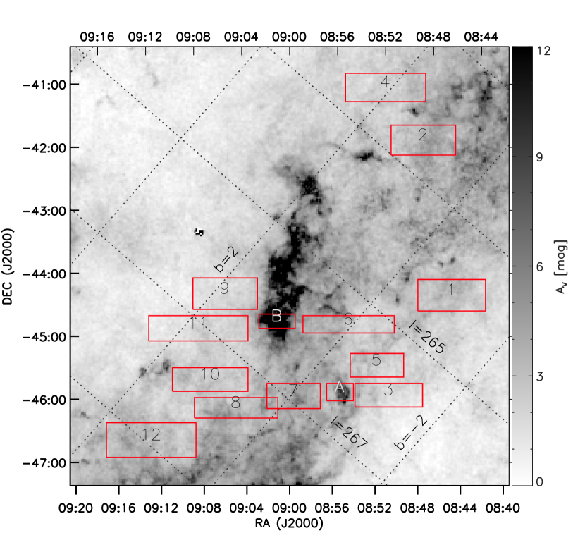
Figure 2.— Like Figure 1 but for the column density from extinction, the color excess $E(J-K_{\rm s})$. The intensity scale has been labeled in $A_{V}$, which is perhaps more intuitive, but as discussed in Section 4 this conversion is only approximate and should not be the basis for quantitative calculations.

The observations were performed by scanning the telescope in azimuth at a speed of $0\fdg 2$ s^-1. The combination of high scan speed and low $1/f$ knee, together with the multiple cross-linking and common-mode removal in the map-maker SANEPIC (Patanchon et al., 2008) retains diffuse low spatial frequency emission (the DC level is removed, however). Ideally the cross-linking scans would have been orthogonal, but solar position constraints resulted in a small angle range, with scans being oriented roughly along constant declination. Consequently small drifts in the baseline produced a low spatial frequency undulation in the cross-scan direction, readily apparent by comparing results from different independent map-makers. We have examined rectangular subregions of sufficiently small dimension in declination to mitigate any potential effects of this artefact (much taller regions were, in fact, examined too and the results were found to be robust).

The subregions examined are shown in Figures 1 and 2 and specified in Table 3. The typical length of a rectangle, $1\arcdeg$, corresponds to 12 pc at the distance of the Vela Molecular Ridge, 700 pc (Murphy & May, 1991). The Galactic latitude range covered by the centers of the different rectangles is $-1\arcdeg$ to $+2\arcdeg$. The maximum separation in longitude is about $7\arcdeg$ (85 pc). The different rectangles sample distinct environments.

Table 1Rectangular regions analyzed

1&8:45:39.5-44:24:22.9264.061-0.868 64.5 $\times$ 30.0
28:48:38.6-41:58:41.9262.511 1.078 61.5 $\times$ 28.5
38:51:00.2-46:02:22.4265.923-1.166 64.5 $\times$ 22.5
48:51:58.6-41:08:50.7262.264 2.087 76.5 $\times$ 27.0
58:52:04.5-45:34:11.9265.680-0.722 51.0 $\times$ 22.5
68:54:42.2-44:55:47.2265.486 0.043 87.0 $\times$ 16.5
78:59:38.4-46:03:41.7266.908-0.036 51.0 $\times$ 24.0
89:04:59.1-46:15:16.4267.666 0.529 79.5 $\times$ 19.5
99:05:48.6-44:25:41.8266.407 1.860 61.5 $\times$ 30.0
109:07:14.3-45:47:51.4267.590 1.126 72.0 $\times$ 22.5
119:08:16.0-44:58:07.5267.101 1.818 94.5 $\times$ 24.0
129:12:53.4-46:42:54.4268.928 1.216 85.5 $\times$ 33.0

A8:55:28.1-46:00:21.9266.394-0.550 25.5 $\times$ 16.5
B9:01:12.0-44:53:13.3266.204 0.943 34.5 $\times$ 13.5

To avoid areas with strong gradients in dust temperature, we concentrated on relatively diffuse regions of moderate brightness, without compact sources, not the high column (and spatial) density molecular clouds where conditions might be less uniform along the line of sight and where the uncertainties in determining the color excess $E(J-K_{\rm s})$ are larger.

However, suspending our caution, we examined in addition two prominent higher column density regions traced even in ¹³CO (Yamaguchi et al., 1999); see rectangles A and B. Netterfield et al. (2009) derived $\sigma_{\rm e}(1200)$ for the clump in rectangle A by comparing the integrated BLAST emission with the mass derived from CO observations (Yamaguchi et al., 1999), providing an independent check on both approaches.

Note that for absolute measures of column density, pixel by pixel, we would have to restore the zero point (DC level) of the BLAST maps, as we did for the Cas A region (Sibthorpe et al., 2009). However, that is not necessary here, since we are exploiting the spatial correlations of dust emission with color excess over the individual rectangles. A corollary is that we obtain the properties of the dust that is producing the spatial variations within each rectangle; a uniform distribution would not be detectable.

3.1. Dust Temperature from the Diffuse Emission

Small scale structures are remarkably well correlated across the three BLAST bands. For a sufficiently large and homogeneous region an estimate of the characteristic temperature can be obtained via pixel-by-pixel correlations of images with respect to some reference image (here BLAST 250 µm). We used the IDL routine SIXLIN to perform the regressions, and adopted the bisector slope as our specific estimator (Isobe et al., 1990). The slopes of these correlations describe the relative SED of the emission that is changing in common in these images.

The SED for cold dust emission at temperature $\sim$ 15 K and emissivity index $\beta=1.8$ peaks at 200 µm, and so in principle the dust temperature could be determined from the curvature in the SED through the three submillimeter passbands of BLAST. Nevertheless, in practice it is always preferable to have broader wavelength coverage, particularly on the short wavelength side of the peak. At the shorter wavelengths we have examined the correlation slope of the 100 µm image from IRAS with BLAST. We used the reprocessed IRIS product (Miville-Deschênes & Lagache, 2005). Because there was a hot point source in rectangle 1 and another in rectangle 4 we used a version of the IRIS images from which the sources have been removed (these hot sources are not prominent at the BLAST passbands). The IRIS 100 µm image has $1\farcm 5$ pixels in common with the other maps used but a lower resolution of about 4′ (Miville-Deschênes et al., 2002). We considered using another IRAS product, the higher resolution HIRES image (Cao et al., 1997). HIRES was originally designed for resolving crowded compact sources (Aumann et al., 1990) and although empirically it improves the resolution of diffuse emission too (e.g., Martin et al., 1994), this has not been quantified at the few percent level. We have, however, convolved the HIRES map (resolution 2′) to the IRIS resolution and correlated it with the original within the rectangles examined. The slope was typically 0.96. We concluded that using IRIS might result in a systematic error of a few percent, but that this was acceptable given the much larger calibration error of 13% (Miville-Deschênes & Lagache, 2005). The effect of such systematic errors is explored in Section 7.4.

An example of the relative SED is shown in Figure 3, for rectangle 7. Note that the fitting function implicitly passes through unity at 250 µm (indicated by a diamond); there is no datum there used explicitly in the fit of the relative SED.

The diffuse emission in the submillimeter and mid-infrared wavelengths comes from two different dust components, distinguished principally by their size distribution, namely Big Grains (BGs) and Very Small Grains (VSGs) (Desert et al., 1990; Li & Draine, 2001; Compiègne et al., 2011). The BGs, in thermal equilibrium with the ambient radiation field, account for most of the dust mass and therefore most of the longer wavelength emission. VSGs are small enough to experience non-equilibrium heating and so broaden the spectrum toward shorter wavelengths, beyond the spectral peak of the BG emission. VSGs comprise a relatively low fraction of the total dust mass, even less in dense regions, and typically their excess emission over what is expected from equilibrium BGs alone appears at 60 µm and shorter wavelengths; in the fields studied here this emission is very faint. Therefore, in this exploratory work we adopted a single temperature SED and fit only data for wavelengths 100 µm and longer, using the IDL routine MPFIT (Markwardt, 2009). Even with fixed $\beta=1.8$, this grey-body functional form provides an acceptable fit to the data (e.g., Figure 3; the best-fit equilibrium temperature for this rectangle is 15.3 $\pm$ 0.4 K).

The observed low slope of the correlation of the 100 µm IRIS image with the 250 µm BLAST image constrains the dust temperature to be low. The degree of correlation between the 100 µm and the 250 µm emission is somewhat less than it is between different BLAST bands. This decorrelation is probably due to a range of grain temperatures within the volume sampled, possibly including a contribution from non-equilibrium emission; temperature changes have non-linear effects in the Wien tail. The correspondingly larger uncertainty in the slope of the correlation, by about a factor two, means that the 100 µm datum has less weight in fitting the SED.

Figure 3.— Relative SED from correlations in rectangle 7 of BLAST and IRIS data with BLAST 250 µm. Implicitly the value is unity at 250 µm (indicated by a diamond); there is no datum there used explicitly in the fit of the relative SED. With $\beta=1.8$ the best fit temperature is 15.3 $\pm$ 0.4 K.

4. Observations of Color Excess

To determine the dust opacity from the submillimeter emission we need an independent tracer of column density, here the near-infrared color excess. This can be estimated using $J$, $H$, and $K_{\rm s}$ data from the 2MASS point source catalog, through a variety of techniques. The color excess map used here was derived by the “AvMAP” procedure which calculates the average near-infrared reddening of stars with a method adapted from earlier analyses (Lada et al., 1994; Lombardi & Alves, 2001; Cambrésy et al., 2002), with improvements as described briefly in Schneider et al. (2006) and more completely in Schneider et al. (2011). For diagnostic purposes, we have used this procedure to produce maps of both $E(J-H)$ and $E(H-K_{\rm s})$. These maps have resolution of about $2\farcm 1$ and $1\farcm 5$ pixels.

We have checked these maps against those more recently published for the whole sky. They correlate well with the extinction maps produced by Rowles & Froebrich (2009) using a median near-infrared color excess technique and with the color excess maps produced by Dobashi (2011) using the “X” percentile method. For example, our $E(H-K_{\rm s})$ compared to that of Dobashi (2011) is $1.08\pm 0.01$ for the moderate column densities of interest in our study (corresponding to $A_{V}$ $<10$), but with considerable deviation beyond that, where extinction is harder to determine.

Our two color excess maps $E(J-H)$ and $E(H-K_{\rm s})$ are very tightly correlated, with a slope of $1.77\pm 0.01$ over a range up to $E(J-K_{\rm s})$ of 5. The rectangles examined here had maximum $E(J-K_{\rm s})$ typically less than a fifth of this value (Table 5.1). Even over the whole field, there is no curvature in the correlation as might be diagnostic of a medium where dense clumps below the resolution limit of “AvMAP” systematically dimmed stars to beyond the completeness limit at $J$ first, biasing $E(J-H)$ to be low.

Theoretically, the $E(J-H)$/$E(H-K_{\rm s})$ ratio is sensitive to the adopted shape of the near-infrared extinction curve, often taken to be a power-law in wavelength (Cardelli et al., 1989; Martin & Whittet, 1990), and to the filter bandpasses and the intrinsic spectra of the stars being measured, because of color corrections which change with increasing extinction. Simulating all of these effects, we find that to explain the observed color excess ratio, the power-law index for near-infrared extinction is $1.85\pm 0.10$, encouragingly close to that found to be common from studies of individual reddened stars (Martin & Whittet, 1990). He et al. (1995) found a ratio of $1.64\pm 0.26$ for highly obscured OB stars with $E(J-K_{\rm s})$ up to about 0.7. Indebetouw et al. (2005) obtained a value of $1.73\pm 0.2$ using various analyses of 2MASS data probing to the much greater column densities accessible in the infrared ($E(J-K_{\rm s})$ up to about 2.5). The region that we have studied is therefore fairly normal, reinforced by the relatively moderate column densities in the rectangles chosen (Table 5.1).

Often near-infrared color excess maps are presented in terms of the more familiar measure of extinction $A_{V}$, via a “total to selective extinction” conversion like

$$A_{V}=R_{XY}E(X-Y).$$ (6)

From studies of individual stars sampling the local diffuse interstellar medium the scaling coefficients frequently adopted, from Rieke & Lebofsky (1985) ignoring the slightly different filter sets, are $R_{HK}=15.87$, $R_{JH}=9.35$, and $R_{JK}=5.89$. Even if the shape of the near-infrared extinction curve were fairly universal, there are significant changes in the shape of the visual to ultraviolet extinction curve, often parameterized in terms of $R_{V}\equiv R_{BV}$, the ratio of total to selective extinction (Cardelli et al., 1989). Increasing $R_{V}$ from 3.1, characteristic of the diffuse interstellar medium, to a value of 5.5, that might be more typical of dark clouds, lowers the scaling coefficients by 20%. Furthermore, there are color corrections at high column densities. We have no direct evidence what scaling to $A_{V}$ would be valid for these Galactic lines of sight toward Vela. Therefore, we decided to use the sum of our two maps, $E(J-K_{\rm s})$, as the best measure of column density, staying close to the directly observable color excesses, mitigating any hidden effects of grain evolution, and more generally avoiding unnecessary, often hidden, assumptions. Of course, $E(J-K_{\rm s})$ still has to be calibrated to give $N_{\rm H}$ (Section 6).

As summarized in Table 3, within the various rectangles measured, $E(J-K_{\rm s})$ ranges typically from 0.24 to 1.1 mag, reaching as low as 0.17 mag in the most diffuse field (rectangle 11) and as high as 3.7 mag toward the main dense cloud in Vela C (rectangle B). In a more familiar metric, these color excesses would correspond to $A_{V}$ = 0.94, 1.4, 6.5, and 22 mag, using the above-mentioned scaling coefficients. However, such scaling needs to regarded with caution, because the high values of color excess and extinction are much beyond those toward stars for which the full infrared to ultraviolet extinction curve, the underlying dust size distribution, and the relationship of $A_{V}$ to color excesses and $N_{\rm H}$ have been studied directly.

5. Emission and Color Excess

Figure 4 illustrates the correlation of $I_{250}$, the continuum emission at 250 µm, with the $E(J-K_{\rm s})$ color excess. Recalling that the dust emission probes the whole line of sight, while the depth to which color excess probes is in principle limited by both attenuation and sensitivity, the correlation is remarkable. The slope of the correlation characterizes the emissivity $\epsilon_{\rm c}(1200)$ of the dust that is causing the spatial variations in column density across the map. The zero point of the BLAST maps is not needed, but by the same token any fairly uniform screen of material cannot be characterized by this correlation technique.

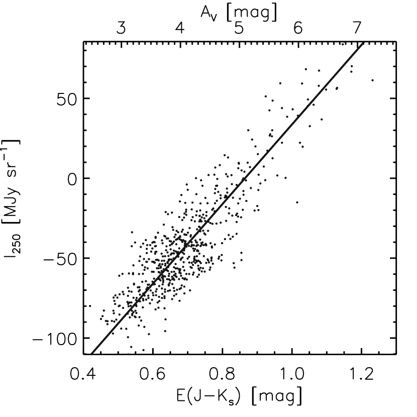
Figure 4.— Pixel-pixel correlation of 250 µm BLAST emission with the color excess $E(J-K_{\rm s})$, in rectangle 7. The solid line has a best-fit slope $\epsilon_{\rm c}(1200)=$ 249.0 $\pm$ 5.0 MJy sr^-1 mag^-1. The $A_{V}$ scale along the top is only approximate, but is provided for context.

The dispersion about the fit in Figure 4 is 0.06 mag if measured horizontally or 16 MJy sr^-1 vertically. We have estimated the error in the $E(J-K_{\rm s})$ map using the scatter about the correlation between the two maps $E(J-H)$ and $E(H-K_{\rm s})$, examined rectangle by rectangle. From this approach, the rms in the $E(J-K_{\rm s})$ map is $\sim$ 0.03 mag. Possibly this is an underestimate because of correlated errors. Therefore, as an alternative we looked at the rms in the adopted $E(J-K_{\rm s})$ map in relatively smooth regions of low color excess and found 0.05 mag; this could overestimate the error because a part is due to real cirrus fluctuations. For comparison with the rms for $I_{250}$ below, 0.03 – 0.05 mag corresponds to 7 – 12 MJy sr^-1. Using similar strategies we have estimated the error in $I_{250}$: from the scatter about the correlation of the $I_{250}$ map with the $I_{350}$ map, rectangle by rectangle, we estimate the rms in $I_{250}$ to be 2 MJy sr^-1; and the rms fluctuation in the dimmest part of the $I_{250}$ map is 3 MJy sr^-1. Returning to Figure 4, our estimates suggest that the error in $E(J-K_{\rm s})$ makes the larger contribution of the two and that taken together there is no compelling reason to require some additional cosmic scatter about the correlation.

The correlations with the other BLAST bands are equally good, but, as foreshadowed by the above cross-band comparisons (Section 3.1), the degree of correlation of 100 µm emission with $E(J-K_{\rm s})$ is less, again possibly due to changes in temperature within the volume probed.

Even though we chose rectangles to avoid strong sources, we explored the possibility that clumpy dust that would contribute to the BLAST emission map might be missed in the sampling of stars underlying the $E(J-K_{\rm s})$ map. We found no evidence for “excess” emission at high color excess even in rectangle B. In the latter rectangle there is possibly a slight deficit, related to clumps of cool dust; in that extreme case our assumption of a constant temperature for dust within the rectangle, rather than systematics in estimating the color excess, is probably the limiting approximation.

5.1. SED

Fitting the slopes of the correlations between dust emission and color excess to a parameterized single-temperature SED yields the dust temperature recorded in Table 5.1. An example is given in Figure 5. These temperatures from the SED fits are around 15 K, definitely cooler than the 17.9 K typical of the high latitude diffuse interstellar medium (Planck Collaboration et al., 2011a). In Table 5.1 we also present the emissivity $\epsilon_{\rm c}(1200)=I_{250}/E(J-K_{\rm s})$, the best-fit amplitudes obtained from the SEDs. Ultimately (Section 7) we will derive the opacity from these observables.

As a consistency check we verified that $T$ derived from the $I_{\nu}$ – $E(J-K_{\rm s})$ correlations here is close to that obtained via the relative SED from the cross-band emission-map correlations (Section 3.1). This supports our premise that relative changes in column density are equally well sampled by changes in BLAST and IRIS emission and in near-infrared excess.

Table 2Dust emission in the Galactic plane toward Vela

ID	$T$	$\epsilon_{\rm c}(1200)$	$r\kappa_{0}$	$\sigma_{\rm e}(1200)$	$P$	$E(J-K_{\rm s})$ range
	K	MJy sr-1 mag-1	cm2 gm-1	10-25 cm2 H-1	$10^{-31}$ W H-1	mag
1	16.8$\pm$ 0.4	202.6$\pm$ 7.6	0.09$\pm$0.01	2.0$\pm$0.2	5.3$\pm$ 0.4	0.25/0.68
2	15.5$\pm$ 0.2	252.1$\pm$ 6.6	0.15$\pm$0.01	3.4$\pm$0.2	5.6$\pm$ 0.2	0.34/0.85
3	15.2$\pm$ 0.5	190.1$\pm$ 11.0	0.12$\pm$0.01	2.8$\pm$0.3	4.0$\pm$ 0.4	0.17/0.59
4	16.2$\pm$ 0.2	265.8$\pm$ 6.1	0.13$\pm$0.01	3.0$\pm$0.1	6.5$\pm$ 0.2	0.24/0.71
5	13.8$\pm$ 0.7	83.8$\pm$ 8.6	0.08$\pm$0.01	1.8$\pm$0.3	1.5$\pm$ 0.3	0.31/0.59
6	14.9$\pm$ 0.2	164.5$\pm$ 4.1	0.11$\pm$0.01	2.6$\pm$0.1	3.4$\pm$ 0.1	0.34/0.85
7	15.2$\pm$ 0.2	230.3$\pm$ 7.2	0.14$\pm$0.01	3.3$\pm$0.2	4.9$\pm$ 0.3	0.51/1.10
8	15.1$\pm$ 0.2	181.6$\pm$ 5.4	0.12$\pm$0.01	2.7$\pm$0.2	3.8$\pm$ 0.2	0.42/0.85
9	15.1$\pm$ 0.2	249.0$\pm$ 7.2	0.16$\pm$0.01	3.7$\pm$0.2	5.3$\pm$ 0.2	0.25/0.59
10	15.2$\pm$ 0.4	124.7$\pm$ 6.6	0.08$\pm$0.01	1.8$\pm$0.2	2.6$\pm$ 0.2	0.34/0.68
11	15.2$\pm$ 0.1	263.6$\pm$ 5.0	0.16$\pm$0.01	3.9$\pm$0.1	5.6$\pm$ 0.2	0.17/0.42
12	15.1$\pm$ 0.2	189.0$\pm$ 4.8	0.12$\pm$0.01	2.8$\pm$0.2	4.0$\pm$ 0.2	0.34/0.81
A	12.4$\pm$ 0.2	75.3$\pm$ 2.9	0.11$\pm$0.01	2.6$\pm$0.2	1.2$\pm$ 0.1	0.42/1.70
B	12.2$\pm$ 0.3	99.9$\pm$ 5.3	0.16$\pm$0.02	3.8$\pm$0.4	1.5$\pm$  0.1	1.19/3.74

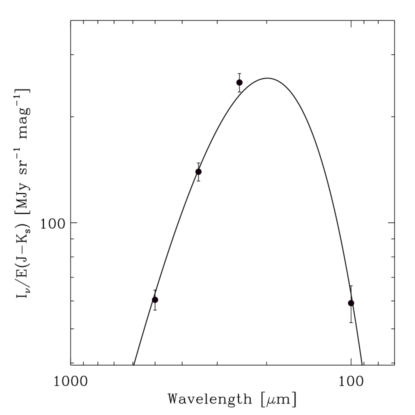
Figure 5.— SED from the slopes of the correlations of dust emission with near-infrared color excess $E(J-K_{\rm s})$ for rectangle 7. The best-fit temperature, 15.2 $\pm$ 0.2 K, is similar to that from the cross-band correlations (Figure 3). The SED amplitude $\epsilon_{\rm c}(1200)$ = 230.3 $\pm$ 7.2 MJy sr^-1 mag^-1 is close to the value obtained from direct correlation (Figure 4).

5.1.1 SED weighting and parameter errors

The slopes of the correlations of BLAST and IRAS with $E(J-K_{\rm s})$, and their uncertainties, were obtained using SIXLIN. For a given rectangle the uncertainties were similar for all BLAST bands and about half of that for the IRAS band. This ratio persisted for all rectangles and so, as in Section 3.1, we have adopted this ratio uniformly in performing weighted SED fits. We consider the systematic effect of calibration errors between BLAST and IRAS in Section 7.4. Here a reduced $\chi^{2}$ of about unity for the fit typically requires an increase of the nominal SIXLIN uncertainties to about 6% and 12% for the BLAST and IRAS bands, respectively. This increase results in more conservative errors on the model parameters $T$ and $\epsilon_{\rm c}(1200)$ (ultimately scaled to $\sigma_{\rm e}(1200)$) and on the dependent quantity $P$ (Equation (5)), as calculated by Monte Carlo simulation (Chapin et al., 2008). A set of 500 realizations of mock data is generated starting with the actual slopes and adding Gaussian noise with the above uncertainties. For each realization the SED was fit and the corresponding parameters recorded. Finally, the uncertainty on each quantity was obtained by fitting a Gaussian to the histogram of the generated distribution. These are the statistical errors reported in Table 5.1. By keeping a record of each fit we also tracked the correlations of the errors and so can produce the elliptical 1-$\sigma$ confidence intervals in, for example, the $T$ – $\sigma_{\rm e}(1200)$ plane (see Section 7.3).

6. Hydrogen Column Density and Color Excess

To calculate the opacity, $\sigma_{\rm e}(\nu)$, we need to relate the color excess $E(J-K_{\rm s})$ to the column density of hydrogen, $N_{\rm{H}}$. Often this is obtained by converting $E(J-K_{\rm s})$ to $A_{V}$ and then using the ratio $N_{\rm{H}}/A_{V}$, all for values found in the local diffuse interstellar medium. This is arguably not justified for the high column density lines of sight where it is applied, and therefore is worthy of some reflection.

$N_{\rm{H}}$ toward individual stars has been measured using Lyman $\alpha$ absorption and the absorption lines of molecular hydrogen using Copernicus and the Far Ultraviolet Spectroscopic Explorer (FUSE) (Bohlin et al., 1978; Savage et al., 1977; Diplas & Savage, 1994; Rachford et al., 2002, 2009). But sensitivity requirements for these ultraviolet measurements have limited the column density probed to $A_{V}$ about 3 mag or $E(J-K_{\rm s})$ about 0.5 mag, lower than in the fields studied here, despite these fields being selected for relatively low column density within the Vela map. If the higher column density here were simply the result of a long line of sight through diffuse material, then it might be argued that the material would be similar to what has been probed directly using individual stars. However, the lines of sight within the rectangles are at least partially molecular (Yamaguchi et al., 1999), and so the material is probably more localized along the line of sight with higher spatial density.

Relating $N_{\rm{H}}$ to $E(B-V)$, these studies of individual stars have found that

$$N_{\rm{H}}=5.8\times 10^{21}E(B-V)\,{\rm cm^{-2}}.$$ (7)

Equation (7) can be recast in terms of $A_{V}$ if $R_{V}$ is known for individual lines of sight, but we think that this is even less appropriate for our application. Evidence for dust evolution on lines of sight passing through dense material comes from changes in the optical-ultraviolet extinction curve (Kim & Martin, 1996 and references therein), which can be parameterized by the changes in $R_{V}$ (Cardelli et al., 1989). Because of this, one might expect deviations from a simple linear relationship between $N_{\rm{H}}$ and $A_{V}$ or even $E(B-V)$, especially for dense regions with high column density. There is an indication of an increase in the slope in the Equation (7) correlation to $6.6\times 10^{21}$ cm^-2 mag^-1 for some higher column density lines of sight ($A_{V}$ of 1 to 5 mag) studied with FUSE (Rachford et al., 2002, 2009). However, it is not known whether this trend is maintained in more dense regions where probing the total hydrogen column density directly is not possible.

Because the ratios of near-infrared color excess to $N_{\rm{H}}$ probably change less significantly as the grains evolve (Martin & Whittet, 1990; Kim & Martin, 1996), it seems advantageous to examine directly the correlation between $N_{\rm{H}}$ and our observable $E(J-K_{\rm s})$.

We used atomic as well as molecular hydrogen column densities measured by Savage et al. (1977) and Rachford et al. (2002, 2009). Below a threshold of $N_{\rm{H}}=0.6\times 10^{21}$ cm^-2, as noted by Savage et al. (1977), the majority of hydrogen is in atomic form. For higher column densities, with a mixture of conditions along the line of sight, our best-fit approximation to the trend in the data above the threshold where both forms of hydrogen are measured is

$$N_{\rm H}=1.52\times(N_{\rm HI}-0.6\times 10^{21})+0.6\times 10^{21}\,{\rm cm^{-2}}.$$ (8)

Diplas & Savage (1994) measured atomic hydrogen along many more lines of sight for which $E(J-K_{\rm s})$ can be obtained, but not molecular hydrogen, and so Equation (8) was used to make a correction. At any column density above the threshold there is dispersion in the fractional amount of hydrogen in molecular form and so this correction is valid only statistically.

For the program stars of Diplas & Savage (1994), we extracted archival 2MASS photometric measurements via GATOR. We concentrated on the $J$ and $K$ bands to maximize the differential extinction and to take advantage of the somewhat better photometry than for the $H$ band. There is a bimodal distribution in the reported photometric uncertainty, the higher peak relating to saturation for the brighter O and B stars. Based on the lower peaks at $J$ and $K$, characterizing the normal photometric error, we have selected those sources which have a combined error in $J-K$ less than $3\sigma_{JK}$, i.e., 0.025 mag. To find the color excess $E(J-K_{\rm s})$ we used the dependence of intrinsic colors on spectral classification given by Straižys & Lazauskaitė (2009).

A preliminary plot of $E(B-V)$ vs. $E(J-K_{\rm s})$ showed that some of these selected program stars are much redder in $E(J-K_{\rm s})$ than could be expected from interstellar extinction. We confirmed from the spectral classification that most of the anomalous stars are known Be or emission-line stars; these have near-infrared emission in addition to that from the photosphere. Hence, to refine our source selection we excluded sources in the color excess plane lying beyond $2.5\sigma$ from the correlation line $E(B-V)/E(J-K_{\rm s})=1.9$; this precaution serves to exclude all of the Be stars from our final list, without unnecessarily biasing our results below.

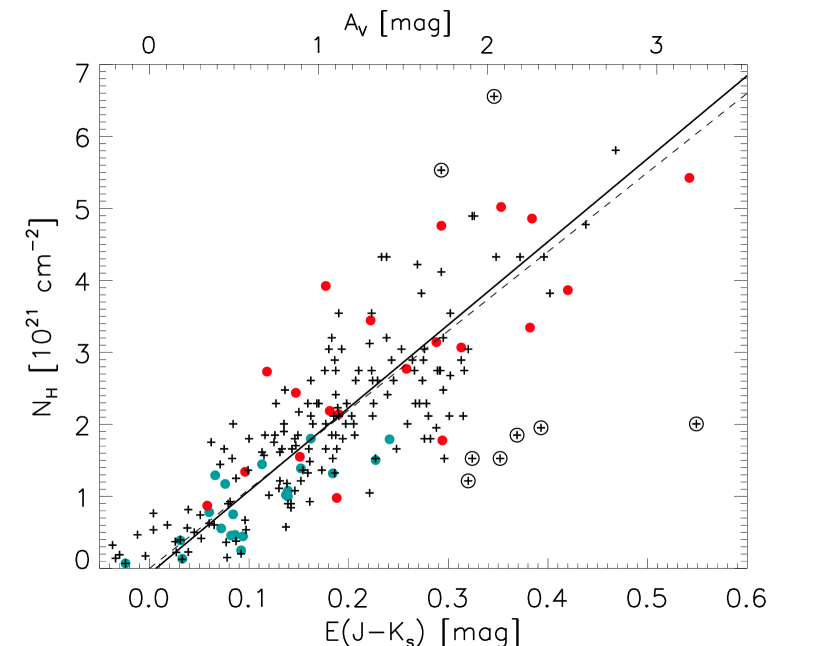
Figure 6.— Correlation between $N_{\rm{H}}$ and $E(J-K_{\rm s})$. Solid green and red circles represent $N_{\rm{H}}$ measurements from Savage et al. (1977) and Rachford et al. (2002, 2009), respectively. Plus symbols are for $N_{\rm{H}}$ from atomic hydrogen measurements by Diplas & Savage (1994), corrected statistically using Equation (8). The best-fit line (solid) has slope ($11.5\pm 0.5)\times 10^{21}$ cm^-2 mag^-1. The dashed line with slope $11.0\times 10^{21}$ cm^-2 mag^-1 is from Equation (7) converted using standard color ratios (see text). Open circles mark the data excluded in the process of iterative fitting. The $A_{V}$ scale along the top is only approximate, but illustrates the limited range covered in this calibration compared to that found in the color excess map in Figure 2, even within the rectangles analyzed.

Figure 6 shows a good correlation between $N_{\rm{H}}$ and $E(J-K_{\rm s})$. We have used an iterative fitting technique to identify and exclude a few outliers more than $3\sigma$ from the correlation. Not surprisingly, and justifying this approach, the outliers are stars from Diplas & Savage (1994), where we have estimated the total hydrogen column density from the atomic hydrogen column density measurements using Equation (8).

The best-fit line is

$$\left(\frac{N_{\rm{H}}}{10^{21}\,{\rm cm^{-2}}}\right)=(11.5\pm 0.5)E(J-K_{\rm s})-0.07\pm 0.01.$$ (9)

For comparison, conversion of the slope in Equation (7) using standard color ratios appropriate to an interstellar extinction curve with $R_{V}=3.1$ (Rieke & Lebofsky, 1985; Cardelli et al., 1989) gives a slope $11.0\times 10^{21}$ cm^-2 mag^-1. This is close to what we have found directly, perhaps reassuringly, but also to some degree coincidentally, given the range of conditions sampled (the converted value would be only half as large for $R_{V}=5.5$). Note the significant dispersion about the average relation.

However, it has only been possible to obtain a direct calibration of this relation to $E(J-K_{\rm s})$ about 0.4 and so applications at higher column densities need to be viewed with caution. This includes the present application, where the top of the $E(J-K_{\rm s})$ range in most rectangles (see Table 5.1) is beyond the calibrated range. On the one hand, to the extent that the larger values are simply the result of longer pathlengths, the calibration should stand. But, on the other hand, if the larger values of $E(J-K_{\rm s})$ are the result of increased volume density then the grains might evolve. For example, calculations of time-dependent extinction curves resulting from grain evolution by ice-mantle formation and aggregation (Ormel et al., 2011) show how $E(J-K_{\rm s})$ might increase for a given column of material, at least initially, which would decrease the ratio $N_{\rm{H}}$/$E(J-K_{\rm s})$. This would in turn raise the derived opacity (Equation (10)), exaggerating the changes reported below.

The same caution about lack of direct calibration also holds for any application which uses such measures of infrared color excess to gauge column density. The situation is further muddied, unnecessarily, when the column density is cited in terms of $A_{V}$.

7. Results

7.1. Opacity at 1200 GHz or 250 µm

Using the temperatures and the amplitudes from the SED fits in Section 5, together with the ratio $N_{\rm{H}}/E(J-K_{\rm s})$ from Section 6, we calculated the opacity from

$$\sigma_{\rm e}(1200)=\epsilon_{\rm c}(1200)/[B_{\nu_{0}}(T)\times N_{\rm{H}}/E(J-K_{\rm s})].$$ (10)

Recall that $\sigma_{\rm e}(1200)\equiv\mu m_{\rm H}r\kappa_{0}$. The derived values are recorded in Table 5.1 along with their Monte Carlo errors (Section 5.1.1). The typical opacity in these regions is about $2.8\times 10^{-25}$ cm² H^-1 or equivalently 0.12 cm² gm^-1. There are considerable variations above what can be accounted for by the errors. Furthermore, all values are significantly above what is typical of the high latitude diffuse interstellar medium, $1.0\times 10^{-25}$ cm² H^-1 (Planck Collaboration et al., 2011a).

Rectangle A coincides with cloud 28 of Yamaguchi et al. (1999) for which Netterfield et al. (2009) have estimated the dust opacity to be $r\kappa_{0}=0.16$ cm² gm^-1 by comparing the integrated submillimeter dust emission with the total mass of gas estimated from the CO emission. The latter introduces an uncertainty of a factor 1.5 – 2. Our new value is $0.11\pm 0.01$ cm² gm^-1.

7.2. Integrated emission

A physical quantity of interest is the total energy emitted by dust per hydrogen atom, $P$ (Equation (5)). For the diffuse high Galactic latitude interstellar medium the value is fairly uniform near $3.8\times 10^{-31}$ W H^-1 (Planck Collaboration et al., 2011a). The typical value found here (see Table 5.1) is somewhat higher, $4.5\times 10^{-31}$ W H^-1. However, not surprisingly, there is considerable variation in the Galactic plane (see also Section 8.2 and Figure 8 below).

7.3. Relationships

The parameters $T$, $\sigma_{\rm e}(1200)$, and $P$ for any rectangle are related at a fundamental level through Equation (5). Because we have used a fixed $\beta=1.8$, this relationship can be quantified as

$$(T/T_{0})^{5.8}=(P/P_{0})\,(\sigma_{\rm e}(1200)/\sigma_{0})^{-1},$$ (11)

using the above-mentioned high latitude diffuse ISM values for normalization (Section 2).

The parameters derived for the different rectangles (Table 5.1) and their elliptical 1-$\sigma$ confidence intervals (Section 5.1.1) are displayed in two complementary diagrams, $T$ – $\sigma_{\rm e}(1200)$ (Figure 7) and $P$ – $\sigma_{\rm e}(1200)$ (Figure 8). These figures include loci according to Equation (11) along which the third parameter is constant. Because of fixed $\beta$ and Equation (11), the third possible diagram, $T$ – $P$, contains no independent new information.

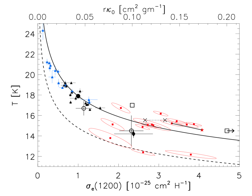
Figure 7.— Dust temperature, $T$, vs. emission opacity, $\sigma_{\rm e}(1200)$. Values for the regions studied here in the Galactic plane toward Vela are represented by the red filled squares with elliptical 1-$\sigma$ confidence intervals. Loci are for constant $P$, the third parameter (Equation (11)): solid, $3.8\times 10^{-31}$ W H^-1 for the diffuse high latitude ISM (Planck Collaboration et al., 2011a); and dashed, three times less. If $\beta$ were fixed at 2.0 in the SED fit, each solution shifts systematically at roughly constant $P$; this is illustrated for rectangle 7 by a line connecting to the star. Also for rectangle 7, the systematic effect of a 15% calibration error between BLAST and IRIS is illustrated by the dotted line segments (see text). The filled circle locates the standard values for the diffuse high latitude ISM (Planck Collaboration et al., 2011a). Values for individual diffuse high latitude regions (Planck Collaboration et al., 2011a) are also plotted, with black and blue distinguishing between LVC and IVC components, respectively. Some further comparisons with empirical results (Appendix B) are plotted. Open circles show Planck results from Planck Collaboration et al. (2011b) toward the Taurus molecular cloud for lines of sight both atomic (upper left) and molecular; the vertical error bars indicate the ranges of temperature. The filled diamond is another estimate for the Taurus region using Spitzer (Terebey et al., 2009). The squares show the range of values found using Herschel data in the environs of a Planck cold clump (Juvela et al., 2011); these results support the trend with $T$ (and column density) established by the other data and extend it to even higher $\sigma_{\rm e}(1200)$ at the highest column densities.

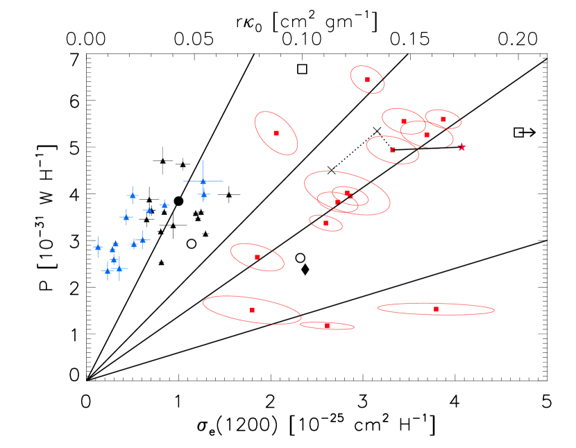
Figure 8.— Like Figure 7 but for power emitted by dust per hydrogen atom, $P$, vs. emission opacity, $\sigma_{\rm e}(1200)$, and with loci (Equation (11)) for different $T$: 13, 15, 16, and 17.9 K from lower to upper.

7.4. Other errors

Throughout this study we have avoided high extinction regions, owing to a larger uncertainty in the color excess and in its conversion to $N_{\rm H}$.

The adopted ratio of $N_{\rm H}/E(J-K_{\rm s})$ might not be universally applicable. A systematic 5% uncertainty in this ratio, or a larger error for individual measurements given the dispersion about the relation (Figure 6; also relevant to Equation (7) which is just the average), induces (inversely) errors of the same size in $\sigma_{\rm e}(1200)$. This is potentially a major contribution to the error budget. While we might have minimized this uncertainty successfully by avoiding high extinction regions, by the same token our derived values of opacity might not be representative of the unanalyzed high extinction regions, including compact sources. Because of the effects of grain evolution mentioned in Section 6 (see also Section 8.3), any application where near-infrared color excess is used to estimate high column densities needs to be assessed critically. We have investigated whether part of the trends seen in Figures 7 and 8 might be induced by changes in $\sigma_{\rm e}(1200)$ originating in a trend of $N_{\rm H}/E(J-K_{\rm s})$ with environment; however, a scatter plot of $\sigma_{\rm e}(1200)$ vs. the average $<E(J-K_{\rm s})>$ for the different rectangles shows no definitive trend, as can be judged by inspection of Table 5.1 as well.

We kept the rectangles fairly small so that the assumption of a uniform temperature for the dust was at least plausible; however, this does not control for temperature changes along the line of sight.

There are calibration errors which could produce systematic effects. For the BLAST bands these are 8.1, 7.1, and 7.8% at 250, 350, and 500 µm, respectively, and by the nature of the calibration technique they are well correlated between the bands (Truch et al., 2009). The calibration error of the IRIS 100 µm image used is 13% (Miville-Deschênes & Lagache, 2005). Because the calibration techniques are independent, there is the possibility of a systematic effect when SEDs are fit to the combined data. If IRIS were adjusted upward, then $T$ would be higher and $\sigma_{\rm e}(1200)$ lower. If instead it were BLAST that was adjusted downward, by the same relative amount, then the same higher $T$ would be found and $\sigma_{\rm e}(1200)$ would be even lower. Such a two-part trajectory is illustrated in the figures for rectangle 7, for a relative calibration error lowering BLAST/IRIS by 15%.

For consistency and comparison to other studies we adopted $\beta=1.8$. The choice of $\beta$ affects the parameters derived from the SED fit in a systematic way. The total power radiated $P$ is quite insensitive to changes in $\beta$, because the SED is required to fit the data across the whole range being integrated. However, both the amplitude and temperature change, the latter affecting the derived opacity more profoundly because of the non-linearity of the Planck function (Equation (10)). For example, if $\beta$ were increased from 1.8 to 2.0, the temperature would be systematically lower and the opacity systematically higher. This shift is illustrated in Figure 7 for rectangle 7. Such effects seem unlikely to account for the much larger values of the opacity found here compared to those in the high latitude interstellar medium. On the contrary, in Appendix A we explore the potential effect of $\beta$ further, in particular through a possible $\beta$ – $T$ relationship, and conclude that this would exaggerate the changes in opacity already found with fixed $\beta$. From this perspective, the estimated magnitude of the changes found and discussed below is conservative.

8. Discussion

There are significant variations from rectangle to rectangle in the derived parameters $T$, $\sigma_{\rm e}(1200)$, and $P$.

For comparison with these new results for the Galactic plane toward Vela, the filled circle in Figures 7 and 8 locates the standard values for the diffuse high Galactic latitude ISM from Planck Collaboration et al. (2011a) that were used to normalize Equation (11). The data plotted for individual diffuse high latitude regions are from SED fits ($\beta=1.8$) to the emissivities reported in Table 2 of Planck Collaboration et al. (2011a), in which local velocity clouds (LVC) and intermediate velocity clouds (IVC) have been separated. Note that the dust emission underlying these SEDs is measured from a combination of Planck and IRIS data. Even at high latitudes there is considerable variation, but interestingly the ranges of $T$ and $\sigma_{\rm e}(1200)$ do not overlap with those found in the present study.

Overall there is a trend in Figure 7 of decreasing $T$ with increasing $\sigma_{\rm e}(1200)$. Although the error ellipses are aligned roughly along this trend, the values span a much larger range than can be attributed to the individual errors of the independent measurements. The range of $P$ in the present study extends to both higher and lower values than seen at high latitudes.

Other estimates discussed in Appendix B are plotted in the figures. These support the trend of decreasing $T$ with increasing $\sigma_{\rm e}(1200)$ seen above.

It is useful to think of Equation (11) in terms of cause (on the right hand side) and effect, $T$. The $P$ calculated here is for emission by big grains in thermal equilibrium and is therefore also the total power absorbed by these grains when exposed to the interstellar radiation field (ISRF). The opacity $\sigma_{\rm e}(1200)$ measures an intrinsic property of the big grains, how efficiently they can emit. This emission opacity and the absorbed $P$ that needs to be emitted determine what the equilibrium $T$ must be. Thus it can be seen that big grains will be cooler in a less intense ISRF, and/or if they were to evolve to have a lower absorption opacity and/or a larger emission opacity.

Here we examine the evidence for such changes using the complementary diagnostic Figures 7 and 8. Considering $T$ as an effect, we concentrate further discussion on the causes, $\sigma_{\rm e}(1200)$ and $P$.

8.1. Changes in $\sigma_{\rm e}(1200)$

A main goal of this paper was to quantify the dust emission opacity in a new environment near the Galactic plane, that is of higher column density than the high latitude ISM, and at least partly molecular. We have found that in this environment $\sigma_{\rm e}(1200)$ is higher by typically a factor three and, extending the finding by Planck Collaboration et al. (2011a), it changes from region to region.

Changes in the emission opacity are certainly intriguing but not understood. One possibility is that the opacity is raised when grains aggregate, changing the basic structure to something more porous and fractal than homogeneous (Ossenkopf & Henning, 1994). This has been discussed for dense molecular clouds, where grains also develop ice mantles (Ormel et al., 2011), but its relevance to such evolutionary changes occurring even within the more diffuse medium seems less obvious. Perhaps one needs a change in perspective on the direction of grain evolution, regarding the higher values found here as “normal” for dense regions and the lower values as the result of evolution of dust back toward a different state in the diffuse interstellar medium. See Jones (2009) for a related discussion on extinction curves.

8.2. Changes in $P$

One of the possible reasons for the range of values of $P$ is variation of the interstellar radiation field (ISRF) in the Galactic plane. Attenuation in dense molecular clouds seems the likely cause of the lower $P$ in rectangles A and B. Likewise, it is at least plausible that the ISRF is higher in those regions (rectangles 2, 4, 9, 11) with $P$ significantly larger than $5\times 10^{-31}$ W H^-1. However, as can be seen from Table 5.1, a scatter plot of $P$ vs. the average $<E(J-K_{\rm s})>$ for the different rectangles does not show any definitive trend.

Especially for rectangles A and B, with the most extreme conditions, we have to be aware of other additional uncertainties, such as $N_{\rm{H}}$/$E(J-K_{\rm s})$ being different than adopted; a decrease in this ratio (Section 6) would raise both the derived $\sigma_{\rm e}(1200)$ and $P$ (deduced from the emission) proportionately, at constant $T$ (lines in Figure 8).

Another factor is grain evolution. If grains are evolving enough to change the emission opacity $\sigma_{\rm e}(1200)$ significantly, it is at least plausible that the capacity to absorb is also changing. However, there are no near-infrared to ultraviolet extinction curves from which to quantify such changes. The evolutionary effects are important to understand because the absorption opacity directly affects the power absorbed from the ISRF and hence $P$ observed in emission. For the typical sizes of big grains in the diffuse interstellar medium, the absorption cross section is approaching the geometric cross section. With grain growth by accretion and aggregation, this ratio of cross sections saturates at a value near unity. Grain growth also increases the mass faster than the geometric cross section, driving down the absorption opacity. Modeling these competing effects would take a detailed grain model and theory of grain evolution, as well as an accounting of the spectral shape of the (attenuated) ISRF, well beyond the scope of this paper.

Another potential factor is the dust-to-gas mass ratio. All of the fields with data in these figures are at the solar Galactocentric distance, and so the underlying metallicity is likely the same. Furthermore, the depletion is already high in the diffuse ISM, leaving little room for dust mass to increase in more dense regions; however, ice signatures do appear in molecular clouds. On the other hand, there is independent evidence for reduced depletion in some IVCs, which would lower both $\sigma_{\rm e}(1200)$ and $P$ at constant $T$. There is a hint of such an effect in Figure 8.

8.3. Insight from theoretical modeling of grain evolution

The emission cross section of dust grains in high latitude diffuse interstellar clouds is better constrained empirically than in translucent (A_V in the range of 1 to 5 mag) or dense molecular clouds (Appendix B).

In their comprehensive review of existing empirical estimates, Henning et al. (1995) comment that “This large scatter [in submillimeter opacities] is very probably not only related to problems with the observational determination of the opacities but may also reflect real differences of the dust populations in different environments caused by evolutionary effects (e.g., coagulation or accretion of mantles).” This has motivated modeling of the grain evolution and the attendant changes in opacity. After reviewing their theoretical calculations relating to the evolution (ice mantles: Preibisch et al., 1993; mantles and coagulation: Ossenkopf & Henning, 1994), Henning et al. (1995) recommended values for three notional environments with the opacity increasing in magnitude from the diffuse interstellar medium (Draine & Lee, 1984; like current estimates) to protostellar cloud envelopes ($n_{\rm H}\sim 10^{5}$ cm^-3, Preibisch et al., 1993; like the values found here for less dense molecular regions) and even further in dense and cold cores ($n_{\rm H}>10^{7}$ cm^-3, Ossenkopf & Henning, 1994; conditions well beyond what is probed here). Although it is acknowledged that the models are instructive rather than definitive, the theoretical estimates have often been adopted for the analysis of submillimeter data because of the lack of empirically-calibrated opacities for these environments; the situation is improving somewhat (Appendix B) but the most dense and evolved regions remain challenging.

With deeper targeted surveys of individual clouds using infrared cameras, some variations of the ratio $E(J-H)$/$E(H-K_{\rm s})$ have been found, suggestive of grain evolution. For example, the ratio found is $1.76\pm 0.07$ in the $\rho$ Oph cloud (Kenyon et al., 1998), $1.96\pm 0.04$ in the Cham I cloud (Gómez & Kenyon, 2001), and $2.25\pm 0.07$ in Coalsack Globule 2 (Racca et al., 2002). In these investigations, $E(J-K_{\rm s})$ ranged up to 5.65, 3.04, and 2.44, respectively, all well beyond the top values in the rectangles considered here. As emphasized in Section 5, $N_{\rm H}/E(J-K_{\rm s})$ has not been calibrated directly for such high column densities.

The multi-wavelength complexity is highlighted by the recent calculations by Ormel et al. (2011), motivated by evidence for changes in the near-infrared extinction for inferred column densities up to $N_{\rm H}\sim 6\times 10^{22}$ cm^-2 (notionally $A_{V}$ $\sim 32$ mag), again well beyond that probed here. Following the effects of ice-mantle formation and (subsequent) grain coagulation, they model the opacity across the whole spectrum from the ultraviolet to submillimeter. As with the earlier models, these results show how the evolution can produce not only increases in submillimeter opacity but also accompanying dramatic changes in the near-infrared and ultraviolet opacity.

The combined effects of magnitude and slope changes in the near-infrared opacity can alter $N_{\rm H}/E(J-K_{\rm s})$. Depending on the model, significant near-infrared changes might develop even before a substantial change in submillimeter opacity. In the Vela region that we have analyzed above there is no change in the infrared slope, and assuming no change in the absolute amount of the extinction either (Section 6) we find that there is an increase in submillimeter opacity relative to that in the diffuse interstellar medium. If the magnitude of the infrared opacity, which we cannot measure directly (but see Figure 6), has actually increased, then the derived opacity would be even higher (see Equation (10)).

The Ormel et al. (2011) results also show a decrease in optical-ultraviolet opacity as the grains evolve, a reminder that $A_{V}$ might not be a good surrogate of column density in these evolved regions. This optical-ultraviolet opacity decrease would decrease the energy absorbed and thus the observed $P$ in emission. However, depending on the details of the evolution, its time development, and the spectral shape of the radiation field, this decrease might be compensated by an increase in the near-infrared opacity. As discussed above, a mis-calibration of $N_{\rm H}/E(J-K_{\rm s})$ would scale $P$ and $\sigma_{\rm e}(1200)$ equally, moving the derived quantities along lines of constant $T$ in Figure 8.

9. Conclusion

We have correlated the diffuse interstellar dust emission in the Galactic plane toward Vela (BLAST images at 250, 350, and 500 µm and the IRAS image at 100 µm) with a map of near-infrared color excess made using 2MASS data. Fourteen regions of moderate column density were analyzed. The conversion of color excess to column density has been examined critically. From stellar data we have measured $N_{\rm H}$/$E(J-K_{\rm s})$ to be $11.5\times 10^{21}$ cm² mag^-1 with a considerable dispersion (Figure 6). From the spectral energy distribution of the dust emission, we have quantified important properties of the big grains, namely the equilibrium temperature $T$ of the big grains that are in thermal equilibrium with the interstellar radiation field (ISRF), their submillimeter opacity $\sigma_{\rm e}(1200)$ (the emission cross section per H nucleon), and $P$, the total power radiated per H nucleon. We find that:

1. The submillimeter opacity is consistently larger than for dust in the local high Galactic latitude interstellar medium, by a factor 2 to 4 relative to the standard $\sigma_{\rm e}(1200)=1.0\times 10^{-25}$ cm² H^-1 value ($r\kappa_{0}=0.043$ cm² gm^-1). This is strong evidence for grain evolution.

2. The range of $P$ extends to both higher and lower values compared to that found at high latitudes, $3.8\times 10^{-31}$ W H^-1 (1.2 L_⊙/M_⊙). This range in part reflects variations in the interstellar radiation field. It is also influenced by evolutionary changes in the dust absorption opacity. In turn, all of the above changes lead to changes in the observable equilibrium $T$.

3. Compared to the local high latitude dust temperature (17.9 K), in this direction in the Galactic plane the dust temperatures are significantly colder, typically 15 K. Somewhat lower temperatures still are found in more dense higher column density regions where the ISRF is more strongly attenuated.

4. Continuing the trend found in high latitude fields, there is an inverse correlation of $T$ with $\sigma_{\rm e}(1200)$.

The recognition that there are changes in the emission opacity raises a particular point of caution, because the value adopted impacts directly all column densities deduced from dust emission maps, and the masses of compact structures (clumps, cores, filaments, ridges) within them. While values typically being adopted (see Appendix B) are within the range that we find, we will need to understand the underlying causes of the variations already observed in order to assess whether there are further changes to be expected in the important even denser environments where the opacity has not been calibrated.

Appendix A Exploration of the Impact of a $\beta$ – $T$ Relationship

There is a considerable literature on a possible inverse relationship between $\beta$ and $T$. However, as is clear from the many examples in Figure 3 of Paradis et al. (2010), there is no consensus on the details of this dependence. In practice, we do not have sufficient multi-wavelength data to treat $\beta$ as an additional free parameter in the SED fit; without the fit being well over-constrained, undue sensitivity could develop to the weighting of the data and issues of calibration, for example. Nevertheless, we have gone through the exercise of treating $\beta$ as a free parameter. For our rectangles we found that the values of free-$\beta$ tended to be a bit larger than 1.8, opposite to the lowering of the apparent $\beta$ expected if the SED is broadened because of dust of different temperatures superimposed along the line of sight.

Over all of the regions examined here plus those in Planck Collaboration et al. (2011a) there is a considerable range of $T$ and a suggestion that $\beta$ is inversely related. This trend could be parameterized as

$$\beta/1.8=(T/17.9\,{\rm K})^{-2/3},$$ (A1)

the power-law index being intermediate among the examples summarized by Paradis et al. (2010).

For the purposes of illustration, following this possible trend through to its potential consequences, we have performed SED fits subject to the added constraint of Equation (A1). The derived parameters are displayed in Figure 9. Loci for constant $P$ under the same constraint are plotted for reference. The effect of constraining the SED fit with this $\beta$ – $T$ relationship is systematic. As expected, each solution remains near the same value of $P$ found for fixed $\beta$. However, compared to Figure 7, the values of the other two parameters are spread out over a larger range on either side of the fiducial values corresponding to $\beta=1.8$ and $T_{0}=17.9$ K.

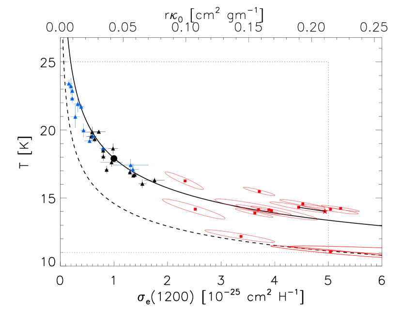
Figure 9.— Dust temperature, $T$, vs. emission opacity, $\sigma_{\rm e}(1200)$, from SED fits under the constraint of the $\beta$ – $T$ relationship in Equation (A1). Loci are for constant $P$ under the same constraint, for the values used in Figure 7. Compared to Figure 7, the solutions for the parameters are spread out over a larger range about the fiducial values corresponding to $\beta=1.8$ and $T_{0}=17.9$ K. However, the increased spread is systematic, each point remaining near the same value of $P$ found for fixed $\beta$. Because of this spreading, the coverage of this figure has been expanded relative to that of Figure 7 (dotted outline) and even so the most extreme points, an IVC and rectangle B, lie off the plot to the upper left and lower right, respectively. For rectangle 7, the star represents the solution obtained when $\beta$ is treated as a free parameter in the SED fit; $\beta$ is found to be 2.2, slightly above the trend described by Equation (A1), and so that solution is similar to the constrained result here.

This spreading exaggerates the differences in $\sigma_{\rm e}(1200)$ found from region to region using fixed $\beta$. We are not actually persuaded that there is a $\beta$ – $T$ relationship, but in any case we conclude that the estimated magnitude of the environmental variations as found for fixed $\beta=1.8$ and discussed in the paper is conservative.

Appendix B Values of Opacity in the Literature

As in Section 2, we standardize on 1200 GHz (250 µm) as the fiducial reference frequency $\nu_{0}$, a value quite appropriate to on-going analyses of Herschel data, for example. The opacity $\sigma_{\rm e}(1200)$ and the product $r\kappa_{0}$ can be used interchangeably through Equation (4), as in the lower and upper axes in Figures 7 and 8; the scale factor between the respective numbers on the axes is 0.043. Scaling to and from the value of opacity at another frequency depends on $\beta$ in which there is some uncertainty; we use $\beta=1.8$. For example, scaling to 1000 GHz lowers the opacity by a factor 1.4.

B.1. Adopted

A value representative of the Preibisch et al. (1993) theoretical core-mantle grain evolution results for conditions in the cloud envelopes of prestellar cores, corresponding to 0.1 cm² gm^-1 at 1000 GHz or $r\kappa_{0}=0.14$ cm² gm^-1, has been adopted by the Herschel Guaranteed Time Key Programs on star formation (Gould Belt Survey, André et al., 2010; HOBYS, Motte et al., 2010), allowing consistent comparisons between different regions analyzed. Whether this is valid for the dense cores extracted is uncertain.

Analyses based on data (only) at lower frequencies, for example by Kerton et al. (2001) for data from SCUBA at JCMT and by Motte et al. (2007) for data from MAMBO at IRAM, often adopt an opacity at a lower fiducial frequency. These are based on theoretical estimates for $n_{\rm H}\sim 10^{5}$ cm^-3 (Ossenkopf & Henning, 1994), and would scale compatibly using to $\beta=2$ to $r\kappa_{0}=0.23$ cm² gm^-1 (or 0.18 cm² gm^-1 for $\beta=1.8$). This is very similar to the value adopted for Herschel because of the closely related theoretical basis.

Analyzing the compact sources in the Science Demonstration Phase (SDP) fields of the Open Time Key Program Hi-GAL (Molinari et al., 2010), Elia et al. (2010) adopted not only a low fiducial frequency (230 GHz) but also a variable $\beta$ in fitting the SEDs; thus comparisons of derived masses are not so straightforward, although effects of $\beta$ on $T$ and the implied $r\kappa_{0}$ somewhat cancel in the mass estimates.

In most BLAST papers on Galactic star forming regions (Chapin et al., 2008; Truch et al., 2008; Rivera-Ingraham et al., 2010; Roy et al., 2011a, b) we adopted $r\kappa_{0}=0.10$ cm² gm^-1 (Hildebrand, 1983; derived empirically from limited observations of a single molecular cloud, for which the value is “probably good within a factor three or four,” this has nevertheless often been adopted as a “canonical” value). In the BLAST analysis of the Vela molecular ridge region (Netterfield et al., 2009; Olmi et al., 2009) we estimated 0.16 cm² gm^-1 using a CO calibration (Section 7.1). For the diffuse interstellar medium toward the CasA supernova remnant (Sibthorpe et al., 2009) we used 0.05 cm² gm^-1. A low value like this is also implicit in any analysis with the standard grains in DustEM (Compiègne et al., 2011).

B.2. Empirical

The value of the opacity for the diffuse high latitude interstellar medium is the best determined, through correlations of the dust emission with $N_{\rm H}$ from observations of the 21 cm emission line. Using observations from DIRBE and FIRAS, Boulanger et al. (1996) obtained an emission cross-section $\sigma_{\rm e}(1200)=1\,\times 10^{-25}$ cm² H^-1, and an equilibrium temperature of 17.5 K, in agreement with the value obtained by Draine & Lee (1984). Also using COBE data, Lagache et al. (1999) found $0.87\pm 0.09\times 10^{-25}$ cm² H^-1, compatible also with the result obtained by Weingartner & Draine (2001). In the text here we cited and plotted $r\kappa_{0}=0.043$ cm² gm^-1 for $T=17.9$ K (Planck Collaboration et al., 2011a). Recently, multi-wavelength analysis of correlations of Planck and IRAS dust maps covering submillimeter to far-infrared wavelengths (Planck Collaboration et al., 2011a) with new higher-resolution observations of $N_{\rm H}$ from the GBT (Boothroyd et al., 2011, Martin et al. in preparation) showed that there were regional variations about this value (see Figure 7). The atomic hydrogen column density associated with these high latitude clouds ranges over $N_{\rm H}\sim 0.2$ to $6\times 10^{20}$ cm^-2 which is equivalent to $A_{V}$ $\sim 0.01$ to 0.3 mag. For the atomic phase in the Taurus field, Planck Collaboration et al. (2011b) obtained a similar opacity $1.14\pm 0.2\times 10^{-25}$ cm² H^-1 using Planck data, for column densities up to $30\times 10^{20}$ cm^-2 ($A_{V}$ about 1.6 mag).

In their Section 5.4.1, Planck Collaboration et al. (2011b) review earlier estimates of opacity in more molecular regions (see also Section 5.2 in Juvela et al., 2011 and Figure 3b in Kramer et al., 2003). For the molecular phase in the same Taurus field they obtained a higher opacity, $2.3\pm 0.3\times 10^{-25}$ cm² H${}^{-1},$ using Planck data and gauging the column density using 21 cm and CO emission-line observations ($N_{\rm H}\sim 1\,\times 10^{22}$ cm^-2). Values for both the atomic phase and molecular phase are plotted in Figure 7; they follow basically the same trend established by the other data, on a locus of slightly lower power (see also Figure 8).

Also in the Taurus region, Terebey et al. (2009) find a similarly higher opacity, by correlating dust optical depth ($T=14.2$ K) from MIPS imaging from Spitzer, extending to 160 µm, with the column density. To estimate the column density they used near-infrared color-excess (which has the same uncertainties as elaborated here in Section 6), making a careful analysis of $A_{V}$. Transforming their 160-µm opacity to our fiducial frequency, we find $\sigma_{\rm e}(1200)=2.1\times 10^{-25}$ cm² H^-1 for $\beta=2$ (2.3 for $\beta=1.8$); see Figures 7 and 8. Flagey et al. (2009) also analyzed similar data over a slightly bigger map in Taurus, finding a very similar temperature and opacity.

With the advent of submillimeter mapping by Planck and Herschel (with zero-point offsets from Planck), SEDs have been fit pixel by pixel, resulting in maps of dust optical depth $\tau$ and $T$. From the slope of $\tau$ versus $N_{\rm H}$ estimated from observations of H I and CO, Bernard et al. (2010) find values $r\kappa_{0}=0.094$ and 0.14 cm² gm^-1 for the Hi-GAL SDP fields at $\ell=59$^∘ and $\ell=30$^∘, respectively.

Dividing the $\tau$ map directly by a map of column density produces a map of opacity (Equation (4)). Note that for this application column density is often obtained by converting a near-infrared color excess (unnecessarily expressed as $A_{V}$) into $N_{\rm H}$ and so the very same caution (Sections 6 and 8.3) as to the lack of direct calibration at high column density applies, even more so. This pixel by pixel approach has the advantage of tracking opacity changes at higher spatial resolution compared to the correlation analyses used here. These spatial changes can be related to changes in $T$ as well, e.g., producing a scatter-plot version of Figure 7. However, it is worth recalling that this method essentially assumes that the properties of the dust ($T$, opacity) are uniform along the line of sight, which might not be the case when the properties are apparently changing significantly in the transverse direction. Mapping the environs of Planck cold clumps with Herschel, Juvela et al. (2011) find opacities typically 0.1 cm² gm^-1 where $T\sim 17$ K ($\beta=2$), but that on the high column density lines of sight $T$ drops to 14.5 K and the opacity rises to 0.2 to 0.3 cm² gm^-1. This again supports the trend found in Figure 7, now on a locus of slightly larger power.

References

- André et al. (2010) André, P., Men’shchikov, A., Bontemps, S., Könyves, V., Motte, F., Schneider, N., Didelon, P., Minier, V., Saraceno, P., Ward-Thompson, D., di Francesco, J., White, G., Molinari, S., Testi, L., Abergel, A., Griffin, M., Henning, T., Royer, P., Merín, B., Vavrek, R., Attard, M., Arzoumanian, D., Wilson, C. D., Ade, P., Aussel, H., Baluteau, J.-P., Benedettini, M., Bernard, J.-P., Blommaert, J. A. D. L., Cambrésy, L., Cox, P., di Giorgio, A., Hargrave, P., Hennemann, M., Huang, M., Kirk, J., Krause, O., Launhardt, R., Leeks, S., Le Pennec, J., Li, J. Z., Martin, P. G., Maury, A., Olofsson, G., Omont, A., Peretto, N., Pezzuto, S., Prusti, T., Roussel, H., Russeil, D., Sauvage, M., Sibthorpe, B., Sicilia-Aguilar, A., Spinoglio, L., Waelkens, C., Woodcraft, A., & Zavagno, A. 2010, A&A, 518, L102
- Aumann et al. (1990) Aumann, H. H., Fowler, J. W., & Melnyk, M. 1990, AJ, 99, 1674
- Bernard et al. (2010) Bernard, J.-P., Paradis, D., Marshall, D. J., Montier, L., Lagache, G., Paladini, R., Veneziani, M., Brunt, C. M., Mottram, J. C., Martin, P., Ristorcelli, I., Noriega-Crespo, A., Compiègne, M., Flagey, N., Anderson, L. D., Popescu, C. C., Tuffs, R., Reach, W., White, G., Benedetti, M., Calzoletti, L., Digiorgio, A. M., Faustini, F., Juvela, M., Joblin, C., Joncas, G., Mivilles-Deschenes, M.-A., Olmi, L., Traficante, A., Piacentini, F., Zavagno, A., & Molinari, S. 2010, A&A, 518, L88
- Bohlin et al. (1978) Bohlin, R. C., Savage, B. D., & Drake, J. F. 1978, ApJ, 224, 132
- Boothroyd et al. (2011) Boothroyd, A. I., Blagrave, K., Lockman, F. J., Martin, P. G., Pinheiro Gonçalves, D., & Srikanth, S. 2011, A&A, 536, A81
- Boulanger et al. (1996) Boulanger, F., Abergel, A., Bernard, J.-P., Burton, W. B., Desert, F.-X., Hartmann, D., Lagache, G., & Puget, J.-L. 1996, A&A, 312, 256
- Cambrésy et al. (2002) Cambrésy, L., Beichman, C. A., Jarrett, T. H., & Cutri, R. M. 2002, AJ, 123, 2559
- Cao et al. (1997) Cao, Y., Terebey, S., Prince, T. A., & Beichman, C. A. 1997, ApJS, 111, 387
- Cardelli et al. (1989) Cardelli, J. A., Clayton, G. C., & Mathis, J. S. 1989, ApJ, 345, 245
- Chapin et al. (2008) Chapin, E. L., Ade, P. A. R., Bock, J. J., Brunt, C., Devlin, M. J., Dicker, S., Griffin, M., Gundersen, J. O., Halpern, M., Hargrave, P. C., Hughes, D. H., Klein, J., Marsden, G., Martin, P. G., Mauskopf, P., Netterfield, C. B., Olmi, L., Pascale, E., Patanchon, G., Rex, M., Scott, D., Semisch, C., Truch, M. D. P., Tucker, C., Tucker, G. S., Viero, M. P., & Wiebe, D. V. 2008, ApJ, 681, 428
- Compiègne et al. (2011) Compiègne, M., Verstraete, L., Jones, A., Bernard, J.-P., Boulanger, F., Flagey, N., Le Bourlot, J., Paradis, D., & Ysard, N. 2011, A&A, 525, A103
- Desert et al. (1990) Desert, F., Boulanger, F., & Puget, J. L. 1990, A&A, 237, 215
- Diplas & Savage (1994) Diplas, A. & Savage, B. D. 1994, ApJS, 93, 211
- Dobashi (2011) Dobashi, K. 2011, PASJ, 63, 1
- Draine & Lee (1984) Draine, B. T. & Lee, H. M. 1984, ApJ, 285, 89
- Dwek et al. (1997) Dwek, E., Arendt, R. G., Fixsen, D. J., Sodroski, T. J., Odegard, N., Weiland, J. L., Reach, W. T., Hauser, M. G., Kelsall, T., Moseley, S. H., Silverberg, R. F., Shafer, R. A., Ballester, J., Bazell, D., & Isaacman, R. 1997, ApJ, 475, 565
- Elia et al. (2010) Elia, D., Schisano, E., Molinari, S., Robitaille, T., Anglés-Alcázar, D., Bally, J., Battersby, C., Benedettini, M., Billot, N., Calzoletti, L., di Giorgio, A. M., Faustini, F., Li, J. Z., Martin, P., Morgan, L., Motte, F., Mottram, J. C., Natoli, P., Olmi, L., Paladini, R., Piacentini, F., Pestalozzi, M., Pezzuto, S., Polychroni, D., Smith, M. D., Strafella, F., Stringfellow, G. S., Testi, L., Thompson, M. A., Traficante, A., & Veneziani, M. 2010, A&A, 518, L97
- Flagey et al. (2009) Flagey, N., Noriega-Crespo, A., Boulanger, F., Carey, S. J., Brooke, T. Y., Falgarone, E., Huard, T. L., McCabe, C. E., Miville-Deschênes, M. A., Padgett, D. L., Paladini, R., & Rebull, L. M. 2009, ApJ, 701, 1450
- Gómez & Kenyon (2001) Gómez, M. & Kenyon, S. J. 2001, AJ, 121, 974
- He et al. (1995) He, L., Whittet, D. C. B., Kilkenny, D., & Spencer Jones, J. H. 1995, ApJS, 101, 335
- Henning et al. (1995) Henning, T., Michel, B., & Stognienko, R. 1995, Planet. Space Sci., 43, 1333
- Hildebrand (1983) Hildebrand, R. H. 1983, QJRAS, 24, 267
- Indebetouw et al. (2005) Indebetouw, R., Mathis, J. S., Babler, B. L., Meade, M. R., Watson, C., Whitney, B. A., Wolff, M. J., Wolfire, M. G., Cohen, M., Bania, T. M., Benjamin, R. A., Clemens, D. P., Dickey, J. M., Jackson, J. M., Kobulnicky, H. A., Marston, A. P., Mercer, E. P., Stauffer, J. R., Stolovy, S. R., & Churchwell, E. 2005, ApJ, 619, 931
- Isobe et al. (1990) Isobe, T., Feigelson, E. D., Akritas, M. G., & Babu, G. J. 1990, ApJ, 364, 104
- Jones (2009) Jones, A. 2009, in EAS Publications Series, Vol. 35, EAS Publications Series, ed. F. Boulanger, C. Joblin, A. Jones, & S. Madden, 3–14
- Juvela et al. (2011) Juvela, M., Ristorcelli, I., Pelkonen, V.-M., Marshall, D. J., Montier, L. A., Bernard, J.-P., Paladini, R., Lunttila, T., Abergel, A., André, P., Dickinson, C., Dupac, X., Malinen, J., Martin, P., McGehee, P., Pagani, L., Ysard, N., & Zavagno, A. 2011, A&A, 527, A111
- Kenyon et al. (1998) Kenyon, S. J., Lada, E. A., & Barsony, M. 1998, AJ, 115, 252
- Kerton et al. (2001) Kerton, C. R., Martin, P. G., Johnstone, D., & Ballantyne, D. R. 2001, ApJ, 552, 601
- Kim & Martin (1996) Kim, S. & Martin, P. G. 1996, ApJ, 462, 296
- Kramer et al. (2003) Kramer, C., Richer, J., Mookerjea, B., Alves, J., & Lada, C. 2003, A&A, 399, 1073
- Lada et al. (1994) Lada, C. J., Lada, E. A., Clemens, D. P., & Bally, J. 1994, ApJ, 429, 694
- Lagache et al. (1999) Lagache, G., Abergel, A., Boulanger, F., Désert, F. X., & Puget, J.-L. 1999, A&A, 344, 322
- Li & Draine (2001) Li, A. & Draine, B. T. 2001, ApJ, 554, 778
- Lombardi & Alves (2001) Lombardi, M. & Alves, J. 2001, A&A, 377, 1023
- Markwardt (2009) Markwardt, C. B. 2009, 411, 251
- Martin et al. (1994) Martin, P. G., Rogers, C., Reach, W. T., Dewdney, P. E., & Heiles, C. E. 1994, in Astronomical Society of the Pacific Conference Series, Vol. 58, The First Symposium on the Infrared Cirrus and Diffuse Interstellar Clouds, ed. R. M. Cutri & W. B. Latter, 188
- Martin & Whittet (1990) Martin, P. G. & Whittet, D. C. B. 1990, ApJ, 357, 113
- Miville-Deschênes & Lagache (2005) Miville-Deschênes, M.-A. & Lagache, G. 2005, ApJS, 157, 302
- Miville-Deschênes et al. (2002) Miville-Deschênes, M.-A., Lagache, G., & Puget, J.-L. 2002, A&A, 393, 749
- Molinari et al. (2010) Molinari, S., Swinyard, B., Bally, J., Barlow, M., Bernard, J., Martin, P., Moore, T., Noriega-Crespo, A., Plume, R., Testi, L., Zavagno, A., Abergel, A., Ali, B., André, P., Baluteau, J., Benedettini, M., Berné, O., Billot, N. P., Blommaert, J., Bontemps, S., Boulanger, F., Brand, J., Brunt, C., Burton, M., Campeggio, L., Carey, S., Caselli, P., Cesaroni, R., Cernicharo, J., Chakrabarti, S., Chrysostomou, A., Codella, C., Cohen, M., Compiegne, M., Davis, C. J., de Bernardis, P., de Gasperis, G., Di Francesco, J., di Giorgio, A. M., Elia, D., Faustini, F., Fischera, J. F., Fukui, Y., Fuller, G. A., Ganga, K., Garcia-Lario, P., Giard, M., Giardino, G., Glenn, J. ., Goldsmith, P., Griffin, M., Hoare, M., Huang, M., Jiang, B., Joblin, C., Joncas, G., Juvela, M., Kirk, J., Lagache, G., Li, J. Z., Lim, T. L., Lord, S. D., Lucas, P. W., Maiolo, B., Marengo, M., Marshall, D., Masi, S., Massi, F., Matsuura, M., Meny, C., Minier, V., Miville-Deschênes, M., Montier, L., Motte, F., Müller, T. G., Natoli, P., Neves, J., Olmi, L., Paladini, R., Paradis, D., Pestalozzi, M., Pezzuto, S., Piacentini, F., Pomarès, M., Popescu, C. C., Reach, W. T., Richer, J., Ristorcelli, I., Roy, A., Royer, P., Russeil, D., Saraceno, P., Sauvage, M., Schilke, P., Schneider-Bontemps, N., Schuller, F., Schultz, B., Shepherd, D. S., Sibthorpe, B., Smith, H. A., Smith, M. D., Spinoglio, L., Stamatellos, D., Strafella, F., Stringfellow, G., Sturm, E., Taylor, R., Thompson, M. A., Tuffs, R. J., Umana, G., Valenziano, L., Vavrek, R., Viti, S., Waelkens, C., Ward-Thompson, D., White, G., Wyrowski, F., Yorke, H. W., & Zhang, Q. 2010, PASP, 122, 314
- Motte et al. (2007) Motte, F., Bontemps, S., Schilke, P., Schneider, N., Menten, K. M., & Broguière, D. 2007, A&A, 476, 1243
- Motte et al. (2010) Motte, F., Zavagno, A., Bontemps, S., Schneider, N., Hennemann, M., di Francesco, J., André, P., Saraceno, P., Griffin, M., Marston, A., Ward-Thompson, D., White, G., Minier, V., Men’shchikov, A., Hill, T., Abergel, A., Anderson, L. D., Aussel, H., Balog, Z., Baluteau, J.-P., Bernard, J.-P., Cox, P., Csengeri, T., Deharveng, L., Didelon, P., di Giorgio, A.-M., Hargrave, P., Huang, M., Kirk, J., Leeks, S., Li, J. Z., Martin, P., Molinari, S., Nguyen-Luong, Q., Olofsson, G., Persi, P., Peretto, N., Pezzuto, S., Roussel, H., Russeil, D., Sadavoy, S., Sauvage, M., Sibthorpe, B., Spinoglio, L., Testi, L., Teyssier, D., Vavrek, R., Wilson, C. D., & Woodcraft, A. 2010, A&A, 518, L77
- Murphy & May (1991) Murphy, D. C. & May, J. 1991, A&A, 247, 202
- Netterfield et al. (2009) Netterfield, C. B., Ade, P. A. R., Bock, J. J., Chapin, E. L., Devlin, M. J., Griffin, M., Gundersen, J. O., Halpern, M., Hargrave, P. C., Hughes, D. H., Klein, J., Marsden, G., Martin, P. G., Mauskopf, P., Olmi, L., Pascale, E., Patanchon, G., Rex, M., Roy, A., Scott, D., Semisch, C., Thomas, N., Truch, M. D. P., Tucker, C., Tucker, G. S., Viero, M. P., & Wiebe, D. V. 2009, ApJ, in press
- Olmi et al. (2009) Olmi, L., Ade, P. A. R., Anglés-Alcázar, D., Bock, J. J., Chapin, E. L., De Luca, M., Devlin, M. J., Dicker, S., Elia, D., Fazio, G. G., Giannini, T., Griffin, M., Gundersen, J. O., Halpern, M., Hargrave, P. C., Hughes, D. H., Klein, J., Lorenzetti, D., Marengo, M., Marsden, G., Martin, P. G., Massi, F., Mauskopf, P., Netterfield, C. B., Patanchon, G., Rex, M., Salama, A., Scott, D., Semisch, C., Smith, H. A., Strafella, F., Thomas, N., Truch, M. D. P., Tucker, C., Tucker, G. S., Viero, M. P., & Wiebe, D. V. 2009, ApJ, 707, 1836
- Ormel et al. (2011) Ormel, C. W., Min, M., Tielens, A. G. G. M., Dominik, C., & Paszun, D. 2011, A&A, 532, A43
- Ossenkopf & Henning (1994) Ossenkopf, V. & Henning, T. 1994, A&A, 291, 943
- Paradis et al. (2010) Paradis, D., Veneziani, M., Noriega-Crespo, A., Paladini, R., Piacentini, F., Bernard, J. P., de Bernardis, P., Calzoletti, L., Faustini, F., Martin, P., Masi, S., Montier, L., Natoli, P., Ristorcelli, I., Thompson, M. A., Traficante, A., & Molinari, S. 2010, A&A, 520, L8
- Pascale et al. (2008) Pascale, E., Ade, P. A. R., Bock, J. J., Chapin, E. L., Chung, J., Devlin, M. J., Dicker, S., Griffin, M., Gundersen, J. O., Halpern, M., Hargrave, P. C., Hughes, D. H., Klein, J., MacTavish, C. J., Marsden, G., Martin, P. G., Martin, T. G., Mauskopf, P., Netterfield, C. B., Olmi, L., Patanchon, G., Rex, M., Scott, D., Semisch, C., Thomas, N., Truch, M. D. P., Tucker, C., Tucker, G. S., Viero, M. P., & Wiebe, D. V. 2008, ApJ, 681, 400
- Patanchon et al. (2008) Patanchon, G., Ade, P. A. R., Bock, J. J., Chapin, E. L., Devlin, M. J., Dicker, S., Griffin, M., Gundersen, J. O., Halpern, M., Hargrave, P. C., Hughes, D. H., Klein, J., Marsden, G., Martin, P. G., Mauskopf, P., Netterfield, C. B., Olmi, L., Pascale, E., Rex, M., Scott, D., Semisch, C., Truch, M. D. P., Tucker, C., Tucker, G. S., Viero, M. P., & Wiebe, D. V. 2008, ApJ, 681, 708
- Planck Collaboration et al. (2011a) Planck Collaboration, Abergel, A., Ade, P. A. R., Aghanim, N., Arnaud, M., Ashdown, M., Aumont, J., Baccigalupi, C., Balbi, A., Banday, A. J., & et al. 2011a, ArXiv e-prints 1101.2036
- Planck Collaboration et al. (2011b) —. 2011b, ArXiv e-prints 1101.2037
- Preibisch et al. (1993) Preibisch, T., Ossenkopf, V., Yorke, H. W., & Henning, T. 1993, A&A, 279, 577
- Racca et al. (2002) Racca, G., Gómez, M., & Kenyon, S. J. 2002, AJ, 124, 2178
- Rachford et al. (2009) Rachford, B. L., Snow, T. P., Destree, J. D., Ross, T. L., Ferlet, R., Friedman, S. D., Gry, C., Jenkins, E. B., Morton, D. C., Savage, B. D., Shull, J. M., Sonnentrucker, P., Tumlinson, J., Vidal-Madjar, A., Welty, D. E., & York, D. G. 2009, ApJS, 180, 125
- Rachford et al. (2002) Rachford, B. L., Snow, T. P., Tumlinson, J., Shull, J. M., Blair, W. P., Ferlet, R., Friedman, S. D., Gry, C., Jenkins, E. B., Morton, D. C., Savage, B. D., Sonnentrucker, P., Vidal-Madjar, A., Welty, D. E., & York, D. G. 2002, ApJ, 577, 221
- Rieke & Lebofsky (1985) Rieke, G. H. & Lebofsky, M. J. 1985, ApJ, 288, 618
- Rivera-Ingraham et al. (2010) Rivera-Ingraham, A., Ade, P. A. R., Bock, J. J., Chapin, E. L., Devlin, M. J., Dicker, S. R., Griffin, M., Gundersen, J. O., Halpern, M., Hargrave, P. C., Hughes, D. H., Klein, J., Marsden, G., Martin, P. G., Mauskopf, P., Netterfield, C. B., Olmi, L., Patanchon, G., Rex, M., Scott, D., Semisch, C., Truch, M. D. P., Tucker, C., Tucker, G. S., Viero, M. P., & Wiebe, D. V. 2010, ApJ, 723, 915
- Rowles & Froebrich (2009) Rowles, J. & Froebrich, D. 2009, MNRAS, 395, 1640
- Roy et al. (2011a) Roy, A., Ade, P. A. R., Bock, J. J., Brunt, C. M., Chapin, E. L., Devlin, M. J., Dicker, S. R., France, K., Gibb, A. G., Griffin, M., Gundersen, J. O., Halpern, M., Hargrave, P. C., Hughes, D. H., Klein, J., Marsden, G., Martin, P. G., Mauskopf, P., Netterfield, C. B., Olmi, L., Patanchon, G., Rex, M., Scott, D., Semisch, C., Truch, M. D. P., Tucker, C., Tucker, G. S., Viero, M. P., & Wiebe, D. V. 2011a, ApJ, 730, 142
- Roy et al. (2011b) Roy, A., Ade, P. A. R., Bock, J. J., Chapin, E. L., Devlin, M. J., Dicker, S. R., France, K., Gibb, A. G., Griffin, M., Gundersen, J. O., Halpern, M., Hargrave, P. C., Hughes, D. H., Klein, J., Marsden, G., Martin, P. G., Mauskopf, P., Morales Ortiz, J. L., Netterfield, C. B., Noriega-Crespo, A., Olmi, L., Patanchon, G., Rex, M., Scott, D., Semisch, C., Truch, M. D. P., Tucker, C., Tucker, G. S., Viero, M. P., & Wiebe, D. V. 2011b, ApJ, 727, 114
- Savage et al. (1977) Savage, B. D., Bohlin, R. C., Drake, J. F., & Budich, W. 1977, ApJ, 216, 291
- Schneider et al. (2006) Schneider, N., Bontemps, S., Simon, R., Jakob, H., Motte, F., Miller, M., Kramer, C., & Stutzki, J. 2006, A&A, 458, 855
- Schneider et al. (2011) Schneider, N., Bontemps, S., Simon, R., Ossenkopf, V., Federrath, C., Klessen, R. S., Motte, F., André, P., Stutzki, J., & Brunt, C. 2011, A&A, 529, A1
- Sibthorpe et al. (2009) Sibthorpe, B., Ade, P. A. R., Bock, J. J., Chapin, E. L., Devlin, M. J., Dicker, S., Griffin, M., Gundersen, J. O., Halpern, M., Hargrave, P. C., Hughes, D. H., Jeong, W., Kaneda, H., Klein, J., Koo, B., Lee, H., Marsden, G., Martin, P. G., Mauskopf, P., Moon, D., Netterfield, C. B., Olmi, L., Pascale, E., Patanchon, G., Rex, M., Roy, A., Scott, D., Semisch, C., Truch, M. D. P., Tucker, C., Tucker, G. S., Viero, M. P., & Wiebe, D. V. 2009, ArXiv e-prints
- Straižys & Lazauskaitė (2009) Straižys, V. & Lazauskaitė, R. 2009, Baltic Astronomy, 18, 19
- Terebey et al. (2009) Terebey, S., Fich, M., Noriega-Crespo, A., Padgett, D. L., Fukagawa, M., Audard, M., Brooke, T., Carey, S., Evans, II, N. J., Guedel, M., Hines, D., Huard, T., Knapp, G. R., McCabe, C.-E., Menard, F., Monin, J.-L., & Rebull, L. 2009, ApJ, 696, 1918
- Truch et al. (2008) Truch, M. D. P., Ade, P. A. R., Bock, J. J., Chapin, E. L., Devlin, M. J., Dicker, S., Griffin, M., Gundersen, J. O., Halpern, M., Hargrave, P. C., Hughes, D. H., Klein, J., Marsden, G., Martin, P. G., Mauskopf, P., Netterfield, C. B., Olmi, L., Pascale, E., Patanchon, G., Rex, M., Scott, D., Semisch, C., Tucker, C., Tucker, G. S., Viero, M. P., & Wiebe, D. V. 2008, ApJ, 681, 415
- Truch et al. (2009) Truch, M. D. P., Ade, P. A. R., Bock, J. J., Chapin, E. L., Devlin, M. J., Dicker, S. R., Griffin, M., Gundersen, J. O., Halpern, M., Hargrave, P. C., Hughes, D. H., Klein, J., Marsden, G., Martin, P. G., Mauskopf, P., Moncelsi, L., Netterfield, C. B., Olmi, L., Pascale, E., Patanchon, G., Rex, M., Scott, D., Semisch, C., Thomas, N. E., Tucker, C., Tucker, G. S., Viero, M. P., & Wiebe, D. V. 2009, ArXiv e-prints
- Weingartner & Draine (2001) Weingartner, J. C. & Draine, B. T. 2001, ApJ, 548, 296
- Yamaguchi et al. (1999) Yamaguchi, N., Mizuno, N., Saito, H., Matsunaga, K., Mizuno, A., Ogawa, H., & Fukui, Y. 1999, PASJ, 51, 775