Finding Density Functionals with Machine Learning

Abstract

Machine learning is used to approximate density functionals. For the model problem of the kinetic energy of non-interacting fermions in 1d, mean absolute errors below 1 kcal/mol on test densities similar to the training set are reached with fewer than 100 training densities. A predictor identifies if a test density is within the interpolation region. Via principal component analysis, a projected functional derivative finds highly accurate self-consistent densities. Challenges for application of our method to real electronic structure problems are discussed.

Each year, more than 10,000 papers report solutions to electronic structure problems using Kohn-Sham (KS) density functional theory (DFT) HK64 ; KS65 . All approximate the exchange-correlation (XC) energy as a functional of the electronic spin densities. The quality of the results depends crucially on these density functional approximations. For example, present approximations often fail for strongly correlated systems, rendering the methodology useless for some of the most interesting problems.

Thus, there is a never-ending search for improved XC approximations. The original local density approximation (LDA) of Kohn and Sham KS65 is uniquely defined by the properties of the uniform gas, and has been argued to be a universal limit of all systems ELCB08 . But the refinements that have proven useful in chemistry SDCF94 and materials PBE96 are not, and differ both in their derivations and details. Traditionally, physicists favor a non-empirical approach, deriving approximations from quantum mechanics and avoiding fitting to specific finite systems PA10 . Such non-empirical functionals can be considered controlled extrapolations that work well across a broad range of systems and properties, bridging the divide between molecules and solids. Chemists typically use a few B88 ; LYP88 or several dozen ZT08 parameters to improve accuracy on a limited class of molecules. Empirical functionals are limited interpolations that are more accurate for the molecular systems they are fitted to, but often fail for solids. Passionate debates are fueled by this cultural divide.

Machine learning (ML) is a powerful tool for finding patterns in high-dimensional data. ML employs algorithms by which the computer learns from empirical data via induction, and has been very successful in many applications mmrts2001 ; i2007 ; RTML12 . In ML, intuition is used to choose the basic mechanism and representation of the data, but not directly applied to the details of the model. Mean errors can be systematically decreased with increasing number of inputs. In contrast, human-designed empirical approximations employ standard forms derived from general principles, fitting the parameters to training sets. These explore only an infinitesimal fraction of all possible functionals and use relatively few data points.

DFT works for electronic structure because the underlying many-body Hamiltonian is simple, while accurate solution of the Schrödinger equation is very demanding. All electrons Coulomb repel one-another, have spin $1/2$, and are Coulomb attracted to the nuclei. ML is a natural tool for taking maximum advantage of this simplicity.

Here, we adapt ML to a prototype density functional problem: non-interacting spinless fermions confined to a 1d box, subject to a smooth potential. We define key technical concepts needed to apply ML to DFT problems. The accuracy we achieve in approximating the kinetic energy (KE) of this system is far beyond the capabilities of any present approximations and is even sufficient to produce highly accurate self-consistent densities. Our ML approximation (MLA) achieves chemical accuracy using many more inputs, but requires far less insight into the underlying physics.

Figure 1: (color online). Comparison of a projected (see within) functional derivative of our MLA with the exact curve.

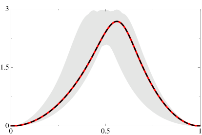
We illustrate the accuracy of our MLA with Fig. 1, in which the functional was constructed from 100 densities on a dense grid. This success opens up a new approach to functional approximation, entirely distinct from previous approaches: Our MLA contains $\sim 10^{5}$ empirical numbers and satisfies none of the standard exact conditions.

The prototype DFT problem we consider is $N$ non-interacting spinless fermions confined to a 1d box, $0\leq x\leq 1$, with hard walls. For continuous potentials $v(x)$, we solve the Schrödinger equation numerically with the lowest $N$ orbitals occupied, finding the KE and the electronic density $n(x)$, the sum of the squares of the occupied orbitals. Our aim is to construct an MLA for the KE $T[n]$ that bypasses the need to solve the Schrödinger equation—a 1d analog of orbital-free DFT KJTH09 . (In (3d) orbital-free DFT, the local approximation, as used in Thomas-Fermi theory, is typically accurate to within 10%, and the addition of the leading gradient correction reduces the error to about 1% DG90 . Even this small an error in the total KE is too large to give accurate chemical properties.)

First, we specify a class of potentials from which we generate densities, which are then discretized on a uniform grid of $G$ points. We use a linear combination of 3 Gaussian dips with different depths, widths, and centers:

$$v(x)=-\sum_{i=1}^{3}a_{i}\exp(-(x-b_{i})^{2}/(2c_{i}^{2})).$$ (1)

We generate 2000 such potentials, randomly sampling $1<a<10$, $0.4<b<0.6$, and $0.03<c<0.1$. For each $v_{j}(x)$, we find, for $N$ up to 4 electrons, the KE $T_{j,N}$ and density $\vectorsym{n}_{j,N}\in\mathbb{R}^{G}$ on the grid using Numerov’s method N24 . For $G=500$, the error in $T_{j,N}$ due to discretization is less than $1.5\times 10^{-7}$. We take 1000 densities as a test set, and choose $M$ others for training. The variation in this dataset for $N=1$ is illustrated in Fig. 2.

Kernel ridge regression (KRR) is a non-linear version of regression with regularization to prevent overfitting htf2009 . For KRR, our MLA takes the form

$$T^{\rm ML}(\vectorsym{n})=\bar{T}\sum_{j=1}^{M}\alpha_{j}k(\vectorsym{n}_{j},\vectorsym{n}),$$ (2)

where $\alpha_{j}$ are weights to be determined, $\vectorsym{n}_{j}$ are training densities and $k$ is the kernel, which measures similarity between densities. Here $\bar{T}$ is the mean KE of the training set, inserted for convenience. We choose a Gaussian kernel, common in ML:

$$k(\vectorsym{n},\vectorsym{n}^{\prime})=\exp(-\|\vectorsym{n}-\vectorsym{n}^{\prime}\|^{2}/(2\sigma^{2})),$$ (3)

where the hyperparameter $\sigma$ is called the length scale. The weights are found by minimizing the cost function

$${\mathcal{C}}(\vectorsym{\alpha})=\sum_{j=1}^{M}\Delta T_{j}^{2}+\lambda\|{\vectorsym{\alpha}}\|^{2},$$ (4)

where $\Delta T_{j}=T^{\rm ML}_{j}-T_{j}$ and $\vectorsym{\alpha}=(\alpha_{1},\dots,\alpha_{M})$. The second term is a regularizer that penalizes large weights to prevent overfitting. The hyperparameter $\lambda$ controls regularization strength. Minimizing ${\mathcal{C}}(\vectorsym{\alpha})$ gives

$$\vectorsym{\alpha}=(\matrixsym{K}+\lambda\matrixsym{I})^{-1}\vectorsym{T},$$ (5)

where $\matrixsym{K}$ is the kernel matrix, with elements $\matrixsym{K}_{ij}=k(\vectorsym{n}_{i},\vectorsym{n}_{j})$, and $\matrixsym{I}$ is the identity matrix. Then $\sigma$ and $\lambda$ are determined through 10-fold cross-validation: The training set is partitioned into 10 bins of equal size. For each bin, the functional is trained on the remaining samples and $\sigma$ and $\lambda$ are optimized by minimizing the mean absolute error (MAE) on the bin. The partitioning is repeated up to 40 times and the hyperparameters are chosen as the median over all bins.

Figure 2: (color online). The shaded region shows the extent of variation of $n(x)$ within our dataset for $N=1$. Exact (red) and a self-consistent (black, dashed) density for potential of Fig. 3.

$N$	$M$	$\lambda\times 10^{14}$	$\sigma$	$\overline{|\Delta T|}$	$|\Delta T|^{\text{std}}$	$|\Delta T|^{\text{max}}$
1	40	$57600$	238	3.3	3.0	23
	60	$10000$	95	1.2	1.2	10
	80	$4489$	48	0.43	0.54	7.1
	100	$12$	43	0.15[3.0]	0.24[5.3]	3.2[46]
	150	$6.3$	33	0.06	0.10	1.3
	200	$3.2$	28	0.03	0.05	0.65
2	100	$1.7$	52	0.13[1.4]	0.20[3.0]	1.8[37]
3	100	$4.0$	74	0.12[0.9]	0.18[1.5]	1.8[14]
4	100	$2.0$	73	0.08[0.6]	0.14[0.8]	2.3[6]
1-4†	400	$3.2$	47	0.12	0.20	3.6

Table 1: Parameters and errors (mean absolute, std. dev., and max abs. in kcal/mol) as a function of electron number $N$ and number of training densities $M$. Brackets represent errors on self-consistent densities with $m=30$ and $\ell=5$. The $\alpha_{j}$ are on the order of $10^{6}$ and both positive and negative suppinfo . ^†Training set includes $\vectorsym{n}_{j,N}$, for $j=1,\dots,100$, $N=1,\dots,4$.

Table 1 gives the performance of $T^{\rm ML}$ (Eq. 2) trained on $M$ $N$-electron densities and evaluated on the corresponding test set. The mean KE of the test set for $N=1$ is 5.40 Hartree (3390 kcal/mol). To contrast, the LDA in 1d is $T^{\rm loc}[n]=\pi^{2}\int dx\,n^{3}(x)/6$ and the von Weizsäcker functional is $T{\rm{}^{W}}[n]=\int dx\,n^{\prime}(x)^{2}/(8n(x))$. For $N=1$, the MAE of $T^{\rm loc}$ on the test set is 217 kcal/mol and the modified gradient expansion approximation LCPB09 , $T^{\rm MGEA}[n]=T^{\rm loc}[n]-c\,T{\rm{}^{W}}[n]$, has a MAE of 160 kcal/mol, where $c=0.0543$ has been chosen to minimize the error (the gradient correction is not as beneficial in 1d as in 3d). For $T^{\rm ML}$, both the mean and maximum absolute errors improve as $N$ or $M$ increases (the system becomes more uniform as $N\to\infty$ ELCB08 ). At $M=80$, we have already achieved “chemical accuracy,” i.e., a MAE below 1 kcal/mol. At $M=200$, no error is above 1 kcal/mol. Simultaneously incorporating different $N$ into the training set has little effect on the overall performance.

With such unheard of accuracy, it is tempting to declare “mission accomplished,” but this would be premature. A KE functional that predicts only the energy is useless in practice, since orbital-free DFT uses functional derivatives in self-consistent procedures to find the density within a given approximation, via

$$\frac{\delta T[n]}{\delta n(x)}=\mu-v(x),$$ (6)

where $\mu$ is adjusted to produce the required particle number. The (discretized) functional derivative of $T^{\rm ML}$ is

$$\frac{1}{\Delta x}\nabla_{\vectorsym}{n}T^{\rm ML}(\vectorsym{n})=\sum_{j=1}^{M}\alpha_{j}^{\prime}(\vectorsym{n}_{j}-\vectorsym{n})k(\vectorsym{n}_{j},\vectorsym{n}),$$ (7)

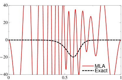
where $\alpha_{j}^{\prime}=\alpha_{j}/(\sigma^{2}\Delta x)$. This oscillates wildly relative to the exact curve (Fig. 3), typical behavior that does not improve with increasing $M$. No finite interpolation can accurately reproduce all details of a functional derivative.

We overcome this problem using principal component analysis (PCA). The space of all densities is contained in $\mathbb{R}^{G}$, but only a few directions in this space are relevant. For a given density $\vectorsym{n}$, find the $m$ training densities $(\vectorsym{n}_{j_{1}},\dots,\vectorsym{n}_{j_{m}})$ closest to $\vectorsym{n}$. Construct the covariance matrix of directions from $\vectorsym{n}$ to each training density $\matrixsym{C}=\matrixsym{X}^{\top}\matrixsym{X}/m,$ where $\matrixsym{X}=(\vectorsym{n}_{j_{1}}-\vectorsym{n},\dots,\vectorsym{n}_{j_{m}}-\vectorsym{n})^{\top}$. Diagonalizing $\matrixsym{C}\in\mathbb{R}^{G\times G}$ gives eigenvalues $\lambda_{j}$ and eigenvectors $\vectorsym{x}_{j}$ which we list in decreasing order. The $\vectorsym{x}_{j}$ with larger $\lambda_{j}$ are directions with substantial variation in the dataset. Those with $\lambda_{j}$ below a cutoff are irrelevant suppinfo . In these extraneous dimensions, there is too little variation within the dataset, producing noise in the model functional derivative. By projecting onto the subspace spanned by the relevant dimensions, we eliminate this noise. This projection is given by $\matrixsym{P}_{m,\ell}(\vectorsym{n})=\matrixsym{V}^{\top}\matrixsym{V},$ where $\matrixsym{V}=(\vectorsym{x}_{1},\dots,\vectorsym{x}_{\ell})^{\top}$ and $\ell$ is the number of relevant eigenvectors. In Fig 1, with $m=30$ and $\ell=5$, the projected functional derivatives are in excellent agreement.

Figure 3: (color online). Functional derivative of $T^{\rm ML}$, evaluated on the density of Fig. 2.

The ultimate test for a density functional is to produce a self-consistent density that minimizes the total energy and check its error. This error will be several times larger than that of the functional evaluated on the exact density. For example, $T^{\rm loc}$ on particles in 1d flat boxes always gives 4 times larger error. To find a minimizing density, perform a gradient descent search restricted to the local PCA subspace: Starting from a guess $\vectorsym{n}^{(0)}$, take a small step in the opposite direction of the projected functional derivative of the total energy in each iteration $j$:

$$\vectorsym{n}^{(j+1)}=\vectorsym{n}^{(j)}-\epsilon\matrixsym{P}_{m,\ell}(\vectorsym{n}^{(j)})(\vectorsym{v}+\nabla_{\vectorsym}{n}T^{\rm ML}(\vectorsym{n}^{(j)})/\Delta x),$$ (8)

where $\epsilon$ is a small number and $\vectorsym{v}$ is the discretized potential. The search is unstable if $\ell$ is too large, inaccurate if $\ell$ is too small, and relatively insensitive to $m$ suppinfo .

The performance of $T^{\rm ML}$ in finding self-consistent densities is given in Table 1. Errors are an order of magnitude larger than that of $T^{\rm ML}$ on the exact densities. We do not find a unique density, but instead a set of similar densities depending on the initial guess (e.g. Fig. 2). The density with lowest total energy does not have the smallest error. Although the search does not produce a unique minimum, it produces a range of similar but valid approximate densities, each with a small error. Even with an order of magnitude larger error, we still reach chemical accuracy, now on self-consistent densities. No existing KE approximation comes close to this performance.

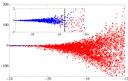
What are the limitations of this approach? ML is a balanced interpolation on known data, and should be unreliable for densities far from the training set. To demonstrate this, we generate a new dataset of 5000 densities with $N=1$ for an expanded parameter range: $0.1<a<20$, $0.2<b<0.8$ and $0.01<c<0.3$. The predictive variance (borrowed from Gaussian process regression rw2006 )

$$\mathbb{V}[T^{\rm ML}(\vectorsym{n})]=k(\vectorsym{n},\vectorsym{n})-\vectorsym{k}(\vectorsym{n})^{\top}(\matrixsym{K}+\lambda\matrixsym{I})^{-1}\vectorsym{k}(\vectorsym{n}),$$ (9)

where $\vectorsym{k}(\vectorsym{n})=(k(\vectorsym{n}_{1},\vectorsym{n}),\dots,k(\vectorsym{n}_{M},\vectorsym{n}))$, is a measure of the uncertainty in the prediction $T^{\rm ML}(\vectorsym{n})$ due to sparseness of training densities around $\vectorsym{n}$. In Fig. 4, we plot the error $\Delta T$ as a function of $\log(\mathbb{V}[T^{\rm ML}(\vectorsym{n})])$, for both the test set and the new dataset, showing a clear correlation. From the inset, we expect our MLA to deliver chemical accuracy for $\log(\mathbb{V}[T^{\rm ML}(\vectorsym{n})])<-24$.

Figure 4: (color online). The correlation between MLA error and predictive variance for $N=1$, $M=100$. Each point represents a density in the test set (blue) or new dataset (red). The vertical line denotes the transition between interpolation and extrapolation.

Does ML allow for human intuition? In fact, the more prior knowledge we insert into the MLA, the higher the accuracy we can achieve. Writing $T=T{\rm{}^{W}}+T_{\theta}$, where $T_{\theta}\geq 0$ KJTH09 , we repeat our calculations to find an MLA for $T_{\theta}$. For $N=1$ we get almost zero error, and a factor of 2-4 reduction of error otherwise. Thus, intuition about the functional can be built in to improve results.

The primary interest in KS DFT is XC for molecules and solids. We have far less information about this than in the prototype studied here. For small molecules and simple solids, direct solutions of the Schrödinger equation yield highly accurate values of $E_{\scriptscriptstyle\rm XC}$. Imagine a sequence of models, beginning with atoms, diatomics, etc., in which such accurate results are used as training data for an MLA. Key issues are how accurate a functional can be attained with a finite number of data, and what fraction of the density space it is accurate for.

A more immediate target is the non-interacting KE in KS DFT calculations. An accurate approximation would allow finding densities and energies without solving the KS equations, greatly increasing the speed of large calculations KJTH09 . The key differences with our prototype is the three-dimensional nature, the Coulomb singularities, and the variation with nuclear positions. For this problem, finding self-consistent densities is crucial, and hence our focus here. But in the 3d case, every KS calculation ever run, including every iteration in a self-consistent loop, generates training data—a density, KE, KS potential and functional derivative. The space of systems, including both solids and molecules, is vast, but could be approached in small steps.

Two last points: The first is that this type of empiricism is qualitatively distinct from that present in the literature. The choices made are those customary in ML, and require no intuition about the physical nature of the problem. Second, the approximation is expressed in terms of about $10^{5}$ numbers, and only the projected functional derivative is accurate. We have no simple way of comparing such approximations to those presently popular. For example, for $N=1$ in the prototype, the exact functional is $T{\rm{}^{W}}$. How is this related to our MLA, and how does our MLA account for this exact limit?

The authors thank the Institute for Pure and Applied Mathematics at UCLA for hospitality and acknowledge NSF CHE-1112442 (JS, KB), EU PASCAL2 and DFG MU 987/4-2 (MR, KH, KRM) and EU Marie Curie IEF 273039 (MR).

References

- (1) P. Hohenberg and W. Kohn, Phys. Rev. B 136, 864 (1964).
- (2) W. Kohn and L. J. Sham, Phys. Rev. A 140, 1133 (1965).
- (3) P. Elliott, D. Lee, A. Cangi, and K. Burke, Phys. Rev. Lett. 100, 256406 (2008).
- (4) P. J. Stephens, F. J. Devlin, C. F. Chabalowski, and M. J. Frisch, J. Phys. Chem. 98, 11623 (1994).
- (5) J. P. Perdew, K. Burke, and M. Ernzerhof, Phys. Rev. Lett. 77, 3865 (1996).
- (6) J. P. Perdew and A. Ruzsinszky, Int. J. Quant. Chem. 110, 2801 (2010).
- (7) A. D. Becke, Phys. Rev. A 38, 3098 (1988).
- (8) C. Lee, W. Yang, and R. G. Parr, Phys. Rev. B 37, 785 (1988).
- (9) Y. Zhao and D. Truhlar, Theor. Chem. Accounts 120, 215 (2008).
- (10) K.-R. Müller, S. Mika, G. Rätsch, K. Tsuda, and B. Schölkopf, IEEE Trans. Neural Network 12, 181 (2001).
- (11) O. Ivanciuc, in Reviews in Computational Chemistry, edited by K. Lipkowitz and T. Cundari (Wiley, Hoboken, 2007), Vol. 23, p. 291.
- (12) M. Rupp, A. Tkatchenko, K.-R. Müller, and O. A. von Lilienfeld, Phys. Rev. Lett. (to be published).
- (13) V. Karasiev, R. Jones, S. Trickey, and F. Harris, in New Developments in Quantum Chemistry, edited by J. Paz and A. Hernández (Research Signpost, Kerala, in press).
- (14) R. M. Dreizler and E. K. U. Gross, Density Functional Theory: An Approach to the Quantum Many-Body Problem (Springer, Berlin, 1990).
- (15) See e.g. E. Hairer, P. Nørsett, P. Syvert Paul and G. Wanner, Solving ordinary differential equations I: Nonstiff problems (Springer, New York, 1993).
- (16) T. Hastie, R. Tibshirani, and J. Friedman, The Elements of Statistical Learning. Data Mining, Inference, and Prediction, 2nd ed. (Springer, New York, 2009).
- (17) See Supplemental Material (appended at the end of this manuscript) for information necessary to construct the MLA functional and more detail on the PCA projections and self-consistent densities.
- (18) D. Lee, L. A. Constantin, J. P. Perdew, and K. Burke, J. Chem. Phys. 130, 034107 (2009).
- (19) C. Rasmussen and C. Williams, Gaussian Processes for Machine Learning (MIT Press, Cambridge, 2006).