A-geometrical approach to Topological Insulators with defects

Abstract

The study of the propagation of electrons with a varying spinor orientability is performed using the coordinate transformation method.

Topological Insulators are characterized by an odd number of changes of the orientability in the Brillouin zone. For defects the change in orientability takes place for closed orbits in real space. Both cases are characterized by nontrivial spin connections.

Using this method , we derive the form of the spin connections for topological defects in three dimensional Topological Insulators.

On the surface of a Topological Insulator, the presence an edge dislocation gives rise to a spin connection controlled by torsion. We find that electrons propagate along two dimensional regions and confined circular contours. We compute for the edge dislocations the tunneling density of states. The edge dislocations violates parity symmetry resulting in a current measured by the in-plane component of the spin on the surface.

I Introduction

The propagation of electrons in solids is characterized by the topological properties of the the electronic band spinors. Topological Insulators Konig ; Volkov ; Gotelman ; Kreutz ; Mele ; Kane ; More ; Essin ; BernewigZhang ; Ludwig ; davidtop ; ZhangField ; Zhangnew can be identified by an odd number of changes of the $orientability$ davidtop of the spinors in the Brillouin zone. As a results non trivial spin connections with a non- zero curvature characterized by the Chern numbers can be identified. In time reversal invariant systems one finds that for Kramer’s states the time reversal operator $T$ obeys $T^{2}=-1$ and one thus the second Chern number for four dimensional space is given by $(-1)^{\nu}=-1$, where $\nu$ is an odd number of orientability changes Nakahara .

Real materials are imperfect and contain topological defects such as dislocations Ran ; Sinova ,disclinations alberto ; Vozmediano and gauge fields induced by strain in graphene Baruch ; Guinea ;therefore, a natural question is to formulate the physics of Topological Insulators in the presence of such defects davidtop . These topological defects can be analyzed using the coordinate transformation method given in ref.kleinert which modifies the Hamiltonian for a Topological Insulator with a defect by the metric tensor and the spin connection Pnueli ; Green ; Birrell ; Randono ; Ryu .

The effect of strain fields dislocations and disclinations plays an important role in material science and can be study using Scanning Tunneling Microscopy ($STM$) and Transmission Electron Spectroscopy ($TEM$ ). Therefore we expect that the chiral metallic boundary Wu will be sensitive to such defects.

In this paper we will introduce the tangent space approach used in differential geometry Nakahara ; Randono ; Ryu to study propagation of electrons for a space dependent coordinate kleinert . We find that the continuum representation of the edge dislocation kleinert generates a spin connection Pnueli ; Green ; Birrell which is controlled by the $Burger$ vector.

Using this formulation we obtain the form of the topological insulator in three dimensions which simplifies for the surface Hamiltonian (on the boundary). For the surface Hamiltonian we find that the electronic excitations are confined to a two-dimensional region and to a set of circular contours of radius $R_{g}(n)$.

The contents of this paper is as follows: In chapter $II$ we introduce the gemetrical method. In section $IIA$ we present the geometrical method for the edge dislocations and strain fields. In section $IIB$ we consider the effects of the strain fields on the three- dimensional Topological Insulator ($TI$). The Chiral model for the boundary surface is presented in section $IIIA$. Section $IIIB$ is devoted to the derivation of the metric tensor and spin connection for an edge dislocation kleinert . In section $IIIC$ we identify the stable solutions. Section $IIID$ is devoted to the stable two dimensional solutions $n=0$ and section $IIIE$ is devoted to the stable solution for circular contours $n=\pm 1$. Chapter $IVA$ is devoted to the computation of the tunneling density of states. In section $IVB$ we present results for the two dimensional region $n=0$. Section $IVC$ is devoted to a large number of dislocations. In section $IVD$ we compute the tunneling density of states for the circular contours $n=\pm 1$. In chapter $V$ we consider the current which is given by the in-plane spin component. In section $VA$ we show that this current is zero for a $TI$. In section $VB$ we show that in the presence of an edge dislocation the parity symmetry is violated, and current, representing the in-plane spin component, is generated. Chapter $VI$ is devoted to conclusions.

II-The Geometrical method for dislocations and strain fields

A-General Considerations

A perfect crystal is described by the lattice coordinates $\vec{r}=[x,y,z]$. For a crystal with a deformation , the coordinates $\vec{r}$ are replaced by $\vec{r}\rightarrow\vec{R}=\vec{r}+\vec{u}\equiv[X^{1}(\vec{r}),X^{2}(\vec{r}),X^{3}(\vec{r})]$ where $\vec{u}(\vec{r})$ is the local lattice deformation and $X^{a}$, $a=1,2,3$ is the local coordinate which changes when we move from one point to another.

In a deformed crystal we introduced a set of local vectors $e_{a}$ which are orthogonal to each other $(e_{b},e_{a})\equiv<e^{b}|e_{a}>=\delta^{b}_{a}$ and local coordinates $X^{a}$, $a=1,2,3$. The unit vector $e_{a}$ can be represented in terms of a Cartesian fixed frame space with the coordinate basis $\partial_{\mu}$ ,$\mu=x,y,z$. In the fixed Cartesian frame the coordinates are given by $x^{\mu}$. Using the Cartesian basis $\partial_{\mu}$ we expand the deformed medium in terms of the local tangent vector $e_{a}$ : $e_{a}=e^{\mu}_{a}\partial_{\mu}$ (for the particular case where vectors $e_{a}$ are given by $e_{a}=\partial_{a}$, the transformation between the two basis is $e^{\mu}_{a}=\delta^{\mu}_{a}$). Any vector $\vec{X}$ (in the deformed space) can be represented in terms of the unit vectors $e_{a}$ or the $\partial_{\mu}$ (the tangent vectors in the Cartesian fixed coordinates space). The vector $\vec{X}$ can be represented in two different ways, $\vec{X}=X^{a}e_{a}=X^{\mu}\partial_{\mu}$ (when an index appear twice is understood as a summation, $X^{a}e_{a}\equiv\sum_{a=1,2,3}X^{a}e_{a}$). The dual vector $e^{a}$ is a $one$ $form$ and can be expanded in terms of the one forms $dx^{\mu}$. We have: $e^{a}=e^{a}_{\mu}dx$, where $e^{a}_{\mu}$ represents the matrix transformation $e^{a}\equiv(\partial_{\mu}X^{a})dx^{\mu}$. The scalar product of the components $e^{a}_{\mu}e^{a}_{\nu}=g_{\mu,\nu}$, $e^{\nu}_{a}e^{\nu}_{b}=\delta_{a,b}$ defines the metric tensors, $g_{\mu,\nu}$ (in the Cartesian frame ) and $\delta_{a,b}$ in the local medium frame.

B-Application to the Topological insulators in three dimensions

The three dimensional electronic $TI$ bands for $Bi_{2}Se_{3}$ and $Bi_{2}Te_{3}$ can be represented using four projected states Chao , $|orbital=1,2>\otimes|spin=\uparrow,\downarrow>$ (the Pauli matrix $\tau$ describes the orbital states and the Pauli matrix $\sigma$ describes the spin). The effective $h^{3D}$ Hamiltonian in the first quantized form is given by:

$$h^{3D}=\hbar v_{0}[k_{y}(\sigma_{1}\otimes\tau_{1})-k_{x}(\sigma_{2}\otimes\tau_{1})+\epsilon k_{z}(\sigma_{3}\otimes\tau_{1})+M(\vec{k})(I\otimes\tau_{3})]$$ (1)

The parameter $M(\vec{k})$ determines if the insulator is trivial or topological. For $Bi_{2}Se_{3}$ and $Bi_{2}Te_{3}$ the gap is inverted, namely $M(\vec{k})=-M_{0}+B_{1}k_{z}^{2}+B_{2}k_{\bot}^{2}$ with $M_{0}>0,B_{1}>0,B_{2}>0$ and therefore topological ZhangField ; Chao ; Zhangnew .

Using the metric tensor $g_{\mu,\nu}$ given by the coordinate transformation ( the transformation between the two sets of coordinates - the one without the dislocation and the second with the dislocation ) $e^{a}_{\mu}e^{a}_{\nu}=g_{\mu,\nu}$, defines the Jacobian $\sqrt{G}$ where $G=det[g_{\mu,\nu}]$. We find that the derivative for a spinor component $\Psi^{(\alpha)}(\vec{r})$, $\alpha=[1=1\uparrow;2=1\downarrow;3=2\uparrow;4=2\downarrow]$ is replaced by the $covariant$ derivative Green :

$$\nabla_{\mu}\Psi^{(\alpha)}(\vec{r})=\partial_{\mu}\Psi^{(\alpha)}(\vec{r})+\frac{1}{8}\omega^{(a,b)}_{\mu}[\hat{\Gamma}^{a},\hat{\Gamma}^{b}]^{\alpha}_{\beta}\Psi^{(\beta)}(\vec{r})$$ (2)

where $\hat{\Gamma}^{a}$ ,$a=1,2,3,4,5$ are the matrixes: $\hat{\Gamma}^{1}=-\Gamma^{2}\equiv-(\sigma_{2}\otimes\tau_{1})$; $\hat{\Gamma}^{2}=\Gamma^{1}\equiv(\sigma_{1}\otimes\tau_{1})$; $\hat{\Gamma}^{3}=\Gamma^{3}\equiv(\sigma_{3}\otimes\tau_{1})$; $\hat{\Gamma}^{4}=\Gamma^{4}\equiv(I\otimes\tau_{2})$;$\hat{\Gamma}^{5}=\Gamma^{5}\equiv(I\otimes\tau_{3})$.

The $spin$ $connection$ $\omega^{a,b}_{\mu}$ determines the covariant derivative Green is given in terms of the tangent vectors $e^{a}_{\mu}$: $e^{a}_{\mu}=\partial_{\mu}X^{a}(\vec{r})$;     $a=1,2,3$ ;     $\mu=x,y,z$.

$$\omega^{a,b}_{\mu}=\frac{1}{2}e^{\nu,a}(\partial_{\mu}e^{b}_{\nu}-\partial_{\nu}e^{b}_{\mu})-\frac{1}{2}e^{\nu,b}(\partial_{\mu}e^{a}_{\nu}-\partial_{\nu}e^{a}_{\mu})$$

$$-\frac{1}{2}e^{\rho,a}e^{\sigma,b}(\partial_{\rho}e_{\sigma,c}-\partial_{\sigma}e_{\rho,c})e^{c}_{\mu}$$ (3)

We notice the asymmetry between $e^{\nu,a}$ and $e_{a,\nu}$: $e^{\nu,a}\equiv g^{\nu,\lambda}e^{a}_{\lambda}$ and $e_{a,\nu}\equiv\delta_{a,b}e^{b}_{\nu}$. As a result the Hamiltonian in eq.$(1)$ in the second quantized form is replaced by:

$$H^{(3D)}=\hbar v_{0}\int\,d^{3}r\sqrt{G}[\Psi^{\dagger}(\vec{r})[e^{\mu}_{a}\hat{\Gamma}^{a}(-i\nabla_{\mu})-E_{F}(I\otimes I)+\hat{\Gamma}^{5}(-M_{0})]\Psi(\vec{r})$$

$$+B_{1}g^{\mu,\nu}(\nabla_{\mu}\Psi^{\dagger}_{1}(\vec{r}))(\nabla_{\nu}\Psi_{1}(\vec{r}))-B_{1}g^{\mu,\nu}(\nabla_{\mu}\Psi^{\dagger}_{2}(\vec{r})\nabla_{\nu}\Psi_{2})]$$

where $e^{\mu}_{a}\hat{\Gamma}^{a}=\sum_{a}e^{\mu}_{a}\hat{\Gamma}^{a}\equiv\hat{\Gamma}^{\mu}(\vec{r})$, $[\hat{\Gamma}^{\mu}(\vec{r})\hat{\Gamma}^{\nu}(\vec{r})+\hat{\Gamma}^{\mu}(\vec{r})\hat{\Gamma}^{\nu}(\vec{r})]=2g^{\mu,\nu}(\vec{r})$ , $det[g^{\mu,\nu}(\vec{r})]\equiv G$ and $\nabla_{\mu}$ is the covariant derivative given in terms of the spin connection given in equation $(2)$: $\nabla_{\mu}\Psi^{(\alpha)}(\vec{r})=\partial_{\mu}\Psi^{(\alpha)}(\vec{r})+\frac{1}{8}\omega^{(a,b)}_{\mu}[\hat{\Gamma}^{a},\hat{\Gamma}^{b}]^{\alpha}_{\beta}\Psi^{(\beta)}(\vec{r})$

C-The Mechanical strain effect on $H^{(3D)}$

From the work of young we learn that the effect of the strained field is different on $Bi_{2}Se_{3}$ than on $Bi_{2}Te_{3}$. In $Bi_{2}Se_{3}$ the $compressive$ strain decreases the Coulombic gap while increasing the inverted gap strength induced by the spin-orbit interaction. We will use the result in equation $(4)$ to analyze the effect of strain. The strain field $\epsilon_{i,j}$ (symmetric in $i,j$) is related to the stress field $\sigma_{i,j}$ and elastic stiffness $Lame$ constant $\lambda$ and $\mu$: $\sigma_{i,j}=\lambda\delta_{i,j}\epsilon_{k,k}+2\mu\epsilon_{i,j}$. Applying a constant stress $\sigma_{i,j}$ one can determine the value of the constant strain field $\epsilon_{i,j}$ which is related to the tangent vectors $e^{i}_{j}\equiv\delta_{i,j}+\epsilon_{i,j}$. In the present case the spin connection and the Christofel tensor vanish. The metric tensor $g_{i,j}$ is given by :$g_{i,j}=\delta_{i,j}+2\epsilon_{i,j}$. Using this formulation we can investigate the effect of the stress on the $Bi_{2}Se_{3}$ at the $\Gamma$ point $\vec{k}=0$. The TI Hamiltonian given in eq.$(4)$ ,$M(\vec{k})=-M_{0}+B_{1}k^{2}_{z}+B_{2}(k^{2}_{x}+k^{2}_{y})$ with the inverted case $M_{0}>0$ Zhangnew . The Hamiltonian in eq. $(4)$ is replaced by:

$$H^{(3D-strain)}=\hbar v_{0}\int\,d^{3}r\sqrt{G}[\Psi^{\dagger}(\vec{r})[\hat{\Gamma}^{a}(\delta_{\mu,a}+\epsilon_{\mu,a})(-i\partial_{\mu}))+\hat{\Gamma}^{4}(-M_{0})+B(1-2\epsilon_{\mu,\nu})\partial_{\mu}\hat{\Gamma}^{4}\partial_{\nu}]\Psi(\vec{r})$$

$$\approx\hbar v_{0}\int\,d^{3}r\sqrt{G}[\Psi^{\dagger}(\vec{r})[\hat{\Gamma}^{a}[(\delta_{\mu,a}(1+<\epsilon>)(-i\partial_{\mu}))]+\hat{\Gamma}^{4}(-M_{0})+B(1-2<\epsilon>\delta_{\mu,\nu})\partial_{\mu}\hat{\Gamma}^{4}\partial_{\nu}]\Psi(\vec{r})$$

In equation $(5)$ we have used the average strain field $<\epsilon>$, $<\epsilon>\equiv\frac{\epsilon_{1,1}+\epsilon_{2,2}+\epsilon_{3,3}}{3}$. We replace the spinor field $\Psi(\vec{r})$ by $\Psi(\vec{r})\sqrt{(1+<\epsilon>)}\equiv\hat{\Psi}(\vec{r})$. As a result we obtain:

$$H^{(3D-strain)}\approx\hbar v_{0}\int\,d^{3}r\sqrt{G}[\hat{\Psi}^{\dagger}(\vec{r})\hat{\Gamma}^{\mu}(-i\partial_{\mu})+\hat{\Gamma}^{4}\frac{(-M_{0})}{(1+<\epsilon>)}+B\frac{(1-2<\epsilon>)}{1+<\epsilon>}\partial_{\mu}\hat{\Gamma}^{4}\partial_{\mu}]\hat{\Psi}(\vec{r})$$

For the compressive case $<\epsilon>$ is negative, $<\epsilon>\equiv-|<\epsilon>|$ . As a result we observe that the inverted gap is enhanced $\frac{|M_{0}|}{(1+<\epsilon>)}=\frac{|M_{0}|}{(1-|<\epsilon>|)}>|M_{0}|$.

In the same way we can show that the Coulomb interaction is reduced: We introduce the Hubbard Stratonovici field $a_{0}$ to describe the Coulomb interactions.

$$H^{e-e}=\int\,d^{3}r\sqrt{G}[I(-e)\cdot a_{0}\Psi^{\dagger}(\vec{r})\Psi(\vec{r})+\frac{(1-2\epsilon_{\mu,\nu})}{2}a_{0}\partial_{\mu}\partial_{\nu}a_{0}]$$

$$\approx\int\,d^{3}r\sqrt{G}[I(-e)\cdot a_{0}\Psi^{\dagger}(\vec{r})\Psi(\vec{r})+\frac{(1-2<\epsilon>)}{2}a_{0}\partial_{\mu}\partial_{\nu}a_{0}]$$

Next we rescale $a_{0}=\frac{A_{0}}{\sqrt{(1-2<\epsilon>)}}$ and obtain:

$$H^{e-e}\approx\int\,d^{3}r\sqrt{G}[I\frac{(-e)}{\sqrt{1-2<\epsilon>}}A_{0}\Psi^{\dagger}(\vec{r})\Psi(\vec{r})+A_{0}\partial_{\mu}\partial_{\mu}A_{0}]$$ (8)

We observe that for the compressive case the effective charge $e_{eff.}\equiv\frac{(-e)}{\sqrt{1-2<\epsilon>}}=\frac{(-e)}{\sqrt{1+2|<\epsilon>|}}$ is reduced and therefore the Coulomb gap decreases, while at the same time the inverted gap increases, $\frac{|M_{0}|}{(1+<\epsilon>)}=\frac{|M_{0}|}{(1-|<\epsilon>|)}>|M_{0}|$ in qualitative agreement with young .

III-The chiral metal with an edge dislocation

A-Description of the Chiral model

The low energy Hamiltonian for the bulk $3D$ $TI$ in the $Bi_{2}Se_{3}$ family was shown to behave on the boundary surface (the $x,y$- plane) as a two dimensional chiral metal nature .

$$H=\int\,d^{2}r\Psi^{\dagger}(\vec{r})[h^{T.I}-\mu]\Psi(\vec{r})]\equiv\hbar v_{F}\int\,d^{2}r\Psi^{\dagger}(\vec{r})[i\sigma^{1}\partial_{y}-i\sigma^{2}\partial_{x}-\mu]\Psi(\vec{r})$$

$h^{T.I}=\hbar v_{F}[i\sigma^{1}\partial_{y}-i\sigma^{2}\partial_{x}]$ is the chiral Dirac Hamiltonian in the first quantized language. $v_{F}\approx 5\cdot 10^{5}\frac{m}{sec}$ is the Fermi velocity, $\sigma$ is the Pauli matrix describing the electron spin and $\mu$ is the chemical potential measured relative to the Dirac $\Gamma$ point. The Hamiltonian for the two dimensional surface $L\times L$ describes well the excitations smaller than the bulk gap of the $3D$ $TI$ at $0.3$ $eV$. Moving away from the $\Gamma$ point, the Fermi velocity becomes momentum dependent; therefore, we will introduce a momentum cut off $\Lambda$ to restrict the validity of the Dirac model. The chiral Dirac model in the Bloch representation takes the form: $h=\hbar v_{F}(\vec{K}\times\vec{\sigma})\cdot\hat{z}\equiv\hbar v_{F}(-\sigma^{1}k_{y}+\sigma^{2}k_{x})$ The eigen-spinors for this Hamiltonian are : $|u(\vec{K})>=[|u_{\uparrow}(\vec{K})>,|u_{\downarrow}(\vec{K})>]^{T}=|\vec{K}>\otimes[1,ie^{i\chi(k_{x},k_{y})}]^{T}$ where $\chi(k_{x},k_{y})=tan^{-1}(\frac{k_{y}}{k_{x}})$ is the spinor phase and $\epsilon=\hbar v_{F}\sqrt{k^{2}_{x}+k^{2}_{y}}$ is the eigenvalue for particles . For holes we have the eigenvalue $\epsilon=-\hbar v_{F}\sqrt{k^{2}_{x}+k^{2}_{y}}$ and eigenvectors $|v(\vec{K})>=[|v_{\uparrow}(\vec{K})>,|v_{\downarrow}(\vec{K})>]^{T}=|\vec{K}>\otimes[-1,ie^{i\chi(k_{x},k_{y})}]^{T}$. The chirality operator is defined in terms of the chiral phase $\chi(k_{x},k_{y})$:

$$(\vec{\sigma}\times\frac{\vec{K}}{|\vec{K}|})\cdot\hat{z}\equiv\sin[\chi(k_{x},k_{y})]\sigma^{1}-\cos[\chi(k_{x},k_{y})]\sigma^{2}$$ (10)

The chirality operator takes the eigenvalue $-$ (counter-clockwise) for particles $[\sin(\chi(k_{x},k_{y}))\sigma^{1}-\cos(\chi(k_{x},k_{y}))\sigma^{2}]|\vec{K}>\otimes[1,ie^{i\chi(k_{x},k_{y})}]^{T}=-|\vec{K}>\otimes[1,ie^{i\chi(k_{x},k_{y})}]^{T}$ and $+$ (clockwise) for holes $[\sin(\chi(k_{x},k_{y}))\sigma^{1}-\cos(\chi(k_{x},k_{y}))\sigma^{2}]|\vec{K}>\otimes[-1,ie^{i\chi(k_{x},k_{y})}]^{T}=|\vec{K}>\otimes[-1,ie^{i\chi(k_{x},k_{y})}]^{T}$.

B-The effect of edge dislocation on a two dimensional chiral surface Hamiltonian

We use the notation $x^{\mu}$ ,$\mu=x,y$ and $X^{a}$ ,$a=1,2$ to describe the media with dislocations. For an edge dislocation in the $x$ direction the $Burger$ vector $B^{(2)}$ is in the $y$ direction . The value of the burger vector $B^{(2)}$ is given by the shortest translation lattice vector in the $y$ direction. (For the $TI$ $Bi_{2}Se_{3}$ the length of the vector $B^{(2)}$ is $5$ times the inter atomic distance ). Following kleinert we introduce the coordinate transformation for an edge dislocation: $\vec{r}=(x,y)\rightarrow[X(\vec{r})=x,Y(\vec{r})=y+\frac{B^{(2)}}{2\pi}\tan^{-1}(\frac{y}{x})]$ with the core of the dislocation centered at $\vec{r}=(0,0)$. The matrix elements fields $e^{a}_{\mu}$ for the edge dislocation is given by :

$$e^{a}_{\mu}=\partial_{\mu}X^{a}(\vec{r});\hskip 7.22743pta=1,2;\hskip 7.22743pt\mu=x,y$$ (11)

We express the Burger vector in terms of the the partial derivatives with respect the coordinates $a=1,2$ in the dislocation frame and $\mu=x,y$ for the fixed Cartesian frame kleinert :

$$\partial_{x}e^{2}_{y}-\partial_{y}e^{2}_{x}=B^{(2)}\delta^{2}(\vec{r})$$ (12)

Using Stokes theorem, we replace the line integral $\displaystyle\oint dx^{\mu}e^{2}_{\mu}(\vec{r})$ by the surface integral $\int\int dx^{\mu}dx^{\nu}[\partial_{x}e^{2}_{y}-\partial_{y}e^{2}_{x}]$. For a system with zero $curvature$ and non zero $torsion$ $T^{(2)}_{\mu,\nu}$ we find that the surface torsion tensor integral $\int\int dx^{\mu}dx^{\nu}T^{(2)}_{\mu,\nu}$ is equal to $\int\int dx^{\mu}dx^{\nu}[\partial_{x}e^{2}_{y}-\partial_{y}e^{2}_{x}]$, and therefore both integrals are equal to the Burger vector.

$$\displaystyle\oint dx^{\mu}e^{2}_{\mu}(\vec{r})=\int\int dx^{\mu}dx^{\nu}[\partial_{\mu}e^{2}_{\nu}-\partial_{\nu}e^{2}_{\mu}]=B^{(2)};$$

$$\int\int dx^{\mu}dx^{\nu}T^{(2)}_{\mu,\nu}=\int\int dx^{\mu}dx^{\nu}[\partial_{\mu}e^{2}_{\nu}-\partial_{\nu}e^{2}_{\mu}]=B^{(2)};$$

where $dx^{\mu}dx^{\nu}$ represents the surface element. The tangent components $e^{a}_{\mu}$ can be expressed in terms of the Burger vector density $B^{(2)}\delta^{2}(\vec{r})$ kleinert :

$$e^{2}_{x}=(\frac{B^{(2)}}{2\pi})\frac{y}{(x^{2}+y^{2})};\hskip 21.68121pte^{2}_{y}=1-(\frac{B^{(2)}}{2\pi})\frac{x}{(x^{2}+y^{2})}$$

$$e^{1}_{x}=1;\hskip 28.90755pte^{1}_{y}=0$$ (14)

Using the tangent components, we obtain the metric tensor $g_{\mu,\nu}$.

$$e^{a}_{\mu}e^{a}_{\nu}\equiv e^{1}_{\mu}e^{1}_{\nu}+e^{2}_{\mu}e^{2}_{\nu}=g_{\mu,\nu}(\vec{r});\hskip 7.22743pte^{a}_{\mu}e^{b}_{\mu}\equiv e^{a}_{x}e^{b}_{x}+e^{a}_{y}e^{b}_{y}=\delta_{a,b}$$ (15)

The inverse of the metric tensor $g_{\mu,\nu}(\vec{r})$ is the tensor $g^{\nu,\mu}(\vec{r})$ defined trough the equation $g_{\mu,\tau}(\vec{r})g^{\tau,\nu}(\vec{r})=\delta_{\mu}^{\nu}$. Using the tangent vectors, we find $to$ $first$ $order$ in the Burger vector the metric tensor $g_{\mu,\nu}$ and the Jacobian transformation $\sqrt{G}$:

$$g_{x,x}=1;\hskip 7.22743ptg_{x,y}=\frac{B^{(2)}}{2\pi}\frac{y}{x^{2}+y^{2}};\hskip 7.22743ptg_{y,y}=1-\frac{B^{(2)}}{2\pi}\frac{y}{x^{2}+y^{2}};\hskip 7.22743ptg_{y,x}=0;\hskip 7.22743ptG=det[g_{\mu,\nu}]=1-\frac{B^{(2)}}{2\pi}\frac{y}{x^{2}+y^{2}}$$ (16)

The inverse tensor is given by:$g^{x,x}\approx 1$, $g^{x,y}=g^{y,x}=-\frac{B^{(2)}}{2\pi}\frac{y}{x^{2}+y^{2}}$, $g^{y,y}=1+\frac{B^{(2)}}{\pi}\frac{x}{x^{2}+y^{2}}$. Using the inverse tensor $g^{\mu,\nu}$ we obtain the inverse matrix $e^{\mu}_{a}$ which is given by:

$$e^{\mu}_{a}=e_{a,\nu}g^{\nu,\mu}=(\delta_{a,b}e^{b}_{\nu})g^{\nu,\mu}=e^{a}_{\nu}g^{\nu,\mu}$$ (17)

Using the components $e^{\mu}_{a}$ we compute the the transformed Pauli matrices. The Hamiltonian in the absence of the edge dislocation is given by $h^{T.I.}=i\gamma^{a}\partial_{a}\equiv\sum_{a=1,2}i\gamma^{a}\partial_{a}$ where the Pauli matrices are given by $\gamma^{1}=-\sigma^{2}$ , $\gamma_{2}=\sigma_{1}$ and $\gamma^{3}=\sigma^{3}$. (We will use the convention that when an index appears twice we perform a summation over this index.) In the presence of the edge dislocation, the term $\gamma^{a}\partial_{a}$ must be expressed in terms of the Cartesian fixed coordinates $\mu=x,y$. As a result, the spinor $\Psi(\vec{r})$ transforms accordingly to the $SU(2)$ transformation . If $\widetilde{\Psi}(\vec{R})$ is the spinor for the deformed lattice, it can be related with the help of an $SU(2)$ transformation to the spinor $\Psi(\vec{r})$ in the undeformed lattice: $\widetilde{\Psi}(X,Y)=e^{-i\frac{\delta\varphi(x,y)}{2}\sigma^{3}}\Psi(x,y)$ . Where $\delta\varphi(x,y)$ is the rotation angle between the two set of coordinates: $\delta\varphi(x,y)=tan^{-1}(\frac{Y}{X})-tan^{-1}(\frac{y}{x})$. Using the relation between the coordinates $X=x$, and $Y=y+\frac{B^{(2)}}{2\pi}tan^{-1}(\frac{y}{x})$ with the singularity at $x=y=0$ gives us that the derivative of the phase which is a delta function, $\partial_{x}\delta\varphi(x,y)=-\partial_{y}\delta\varphi(x,y)\propto\delta^{2}(x,y)$. Combining the transformation of the derivative with the $SO(2)$ rotation in the plane, we obtain the form of the chiral Dirac equation in the Cartesian space (see Appendix A) given in terms of the $spin$ $connection$ $\omega_{\mu}^{1,2}$ Nakahara :

$$i\gamma_{a}\partial_{a}\widetilde{\Psi}(\vec{R})=i\delta_{a,b}\gamma^{b}\partial_{a}\widetilde{\Psi}(\vec{R})=i\gamma^{a}e^{\mu}_{a}[\partial_{\mu}+\frac{1}{4}[\gamma^{b},\gamma^{c}]\omega_{\mu}^{bc}]\Psi(\vec{r})$$ (18)

The Hamiltonian $h^{T.I.}\rightarrow h^{edge}$ is transformed to the dislocation edge Hamiltonian with the explicit form given by:

$$h^{edge}=i\sigma^{1}\partial_{2}-i\sigma^{2}\partial_{1}=i\sigma^{1}e^{\mu}_{2}[\partial_{\mu}+\frac{1}{8}[\sigma^{1},\sigma^{2}]\omega^{1,2}_{\mu}]-i\sigma^{2}e^{\mu}_{1}[\partial_{\mu}+\frac{1}{8}[\sigma^{1},\sigma^{2}]\omega^{1,2}_{\mu}]$$

$$=i(\sigma^{1}e^{\mu}_{2}-\sigma^{2}e^{\mu}_{1})(\partial_{\mu}+\frac{1}{8}[\sigma^{1},\sigma^{2}]\omega^{1,2}_{\mu})$$

To first order in the Burger vector we find : $\omega_{x}^{12}=-\omega_{x}^{21}=0$ and $-\omega_{y}^{21}=\omega_{y}^{1,2}=-\frac{B^{(2)}}{2}\delta^{2}(\vec{r})$, see eqs. $(72-74)$ in Appendix A.

$$h^{edge}\approx i\sigma^{1}(\partial_{y}-\frac{i}{2}\sigma^{3}B^{(2)}\delta^{2}(\vec{r}))-i\sigma^{2}\partial_{x}$$ (20)

In the second quantized form the chiral Dirac Hamiltonian in the presence of an edge dislocations is given by :

$$H^{edge}\approx\int\,d^{2}r\sqrt{G}\Psi^{\dagger}(\vec{r})[h^{edge}-\mu]\Psi(\vec{r})$$

$$\equiv\hbar v_{F}\int\,d^{2}r\sqrt{G}\Psi^{\dagger}(\vec{r})[i\sigma^{1}(\partial_{y}-\frac{i}{2}\sigma^{3}B^{(2)}\delta^{2}(\vec{r}))-i\sigma^{2}\partial_{x}-\mu]\Psi(\vec{r})$$

$h^{edge}$ is the Hamiltonian in the first quantized language, $\mu$ is the chemical potential and $\Psi(\vec{r})=[\Psi_{\uparrow}(\vec{r}),\Psi_{\downarrow}(\vec{r})]^{T}$ is the two component spinor field.

C- The Identification of the physical contours for the edge Hamiltonian $h^{edge}$

In order to identify the solutions, we will use the complex representation. The coordinates in the complex representation are given by, $z=\frac{1}{2}(x+iy)$,    $\overline{z}=\frac{1}{2}(x-iy)$,     $\partial_{z}=\partial_{x}-i\partial_{y}$,     $\partial_{\overline{z}}=\partial_{x}+i\partial_{y}$. In this representation the two dimensional delta function $\delta^{2}(\vec{r})$ is given by $\delta^{2}(\vec{r})\equiv\frac{1}{\pi}\partial_{z}(\frac{1}{\overline{z}})=\frac{1}{\pi}\partial_{\overline{z}}(\frac{1}{z})$ Conformal ; Nair . We will use the edge Hamiltonian $h^{edge}$ and will compute the eigenfunctions $u_{\epsilon}(z,\overline{z})=[U_{\epsilon\uparrow}(z,\overline{z}),U_{\epsilon\downarrow}(z,\overline{z})]^{T}$ and $v_{\epsilon}(z,\overline{z})=V_{\epsilon\uparrow}(z,\overline{z}),V_{\epsilon\downarrow}(z,\overline{z})]^{T}$. The eigenvalue equation is given by:

$$\epsilon U_{\epsilon\uparrow}(z,\overline{z})=-[\partial_{z}+(\frac{B^{(2)}}{\sqrt{2}\pi})\partial_{z}(\frac{1}{\overline{z}})]U_{\epsilon\downarrow}(z,\overline{z})$$

$$\epsilon U_{\epsilon\downarrow}(z,\overline{z})=[\partial_{\overline{z}}+(\frac{B^{(2)}}{\sqrt{2}\pi})\partial_{\overline{z}}(\frac{1}{z})]U_{\epsilon\uparrow}(z,\overline{z})$$

The eigenfunctions $u_{\epsilon}(z,\overline{z})$ and $v_{\epsilon}(z,\overline{z})$ can be written with the help of a singular matrix $M(z,\overline{z})$ Ezawa :

$$u_{\epsilon}(z,\overline{z})=M(z,\overline{z})\hat{F}_{\epsilon}(z,\overline{z})\equiv\left[\begin{array}[]{rrr}e^{-\frac{B^{(2)}}{2\pi}(\frac{1}{z})}&0\\ 0&e^{-\frac{B^{(2)}}{2\pi}(\frac{1}{\overline{z}})}\\ \end{array}\right]\left(\begin{array}[]{cc}F_{\epsilon\uparrow}(z,\overline{z})\\ F_{\epsilon\downarrow}(z,\overline{z})\end{array}\right)$$

($F_{\epsilon}(z,\overline{z})$ and $F_{-\epsilon}(z,\overline{z})$ are the transformed eigenfunctions for $\epsilon>0$ and $\epsilon<0$ respectively .) In terms of the transformed spinors the eigenvalue equation $h^{edge}(z,\overline{z})u_{\epsilon}(z,\overline{z})=\epsilon u_{\epsilon}(z,\overline{z})$ and $F_{\epsilon\downarrow}(z,\overline{z})$ becomes:

$$\epsilon\left(\begin{array}[]{cc}F_{\epsilon\uparrow}(z,\overline{z})\\ F_{\epsilon\downarrow}(z,\overline{z})\end{array}\right)=\left[\begin{array}[]{rrr}I(z,\overline{z})&0\\ 0&(I(z,\overline{z})^{*}\\ \end{array}\right]\left[\begin{array}[]{rrr}-\partial_{z}&0\\ 0&\partial_{\overline{z}}\\ \end{array}\right]\left(\begin{array}[]{cc}F_{\epsilon\uparrow}(z\overline{z})\\ F_{\epsilon\downarrow},(z,\overline{z})\end{array}\right)$$

where $I(z,\overline{z})=e^{-\frac{B^{(2)}}{2\pi}(\frac{\overline{z}-z}{z\overline{z}})}\equiv e^{2\frac{B^{(2)}}{\pi}(\frac{iy}{x^{2}+y^{2}})}$ , $(I(z,\overline{z}))^{*}=e^{2\frac{B^{(2)}}{\pi}(\frac{-iy}{x^{2}+y^{2}})}$, $|I(z,\overline{z})|=1$. We search for zero modes $\epsilon=0$ and find :

$$\partial_{z}F_{\epsilon\downarrow}(z,\overline{z})=0\hskip 36.135pt\partial_{\overline{z}}F_{\epsilon\uparrow}(z,\overline{z})=0$$ (23)

The solutions are given by the holomorphic representation $F_{\epsilon=0\uparrow}(z,\overline{z})=f_{\uparrow}(z)$ and the anti-holomorphic function $F_{\epsilon=0\downarrow}(z,\overline{z})=f_{\downarrow}(\overline{z})$. The zero mode eigenfunctions are given by :

$$u_{\epsilon=0,\uparrow}(z)=e^{-\frac{B^{(2)}}{2\pi}(\frac{1}{z})}f_{\uparrow}(z),\hskip 36.135ptu_{\epsilon=0,\downarrow}(\overline{z})=e^{-\frac{B^{(2)}}{2\pi}(\frac{1}{\overline{z}})}f_{\downarrow}(\overline{z})$$ (24)

Due to the presence of the essential singularity at $z=0$ it is not possible to find analytic functions $f_{\uparrow}(z)$ and $f_{\downarrow}(\overline{z})$ which vanish fast enough around $z=0$ such that $\int d^{2}z(u_{\epsilon=0,\lambda}(z))^{*}u_{\epsilon=0,\lambda}(z)<\infty$. Therefore, we conclude that zero mode solution does not exists. The only way to remedy the problem is to allow for states with finite energy.

In the next step we look for finite energy states. We perform a coordinate transformation :

$$z\rightarrow W[z,\overline{z}];\hskip 36.135pt\overline{z}\rightarrow\overline{W}[z,\overline{z}]$$ (25)

We demand that the transformation is conformal and preserve the orientation. This restricts the transformations to holomorphic and anti-holomorphic functions Conformal . This means that we have the conditions $\partial_{\overline{z}}W[z,\overline{z}]=0$ and $\partial_{z}\overline{W}[z,\overline{z}]=0$. As a result we obtain $W[z,\overline{z}]=W[z]$ and $\overline{W}[z,\overline{z}]=\overline{W}[\overline{z}]$, which obey the eigenvalue equations:

$$\epsilon F_{\epsilon\uparrow}(W,\overline{W})=-\partial_{W}F_{\epsilon\downarrow}(W,\overline{W})$$

$$\epsilon F_{\epsilon\downarrow}(W,\overline{W})=\partial_{\overline{W}}F_{\epsilon\uparrow}(W,\overline{W})$$

This implies the conditions $\frac{dW[z]}{dz}=(I(z,\overline{z}))^{*}$ and $\frac{d\overline{W}[\overline{z}]}{dz}=I(z,\overline{z})$. Since $I(z,\overline{z})$ is neither holomorphic or anti-holomorphic and satisfy $|I(z,\overline{z})|=1$, the only solutions for $W[z]$ and $\overline{W}[\overline{z}]$ must obey $I(z,\overline{z})=1$:

$$I(z,\overline{z})\equiv e^{2\frac{B^{(2)}}{\pi}(\frac{iy}{x^{2}+y^{2}})}=e^{i2\pi n};\hskip 14.45377ptn=0,\pm 1,\pm 2....$$ (27)

For $I(z,\overline{z})\neq 1$ one obtains solutions which are unstable . The stable solutions will be given by a one parameter $s$ curve ($s$ is the length of the curve) $\vec{r}(s)\equiv[x(s),y(s)]$ which obey the equation $I(z,\overline{z})=1$. The curve $\vec{r}(s)$ allows us to define the $tangent$ $\vec{t}(s)$ and the $normal$ vectors $\vec{N}(s)$. This allows us to introduce a two- dimensional region in the vicinity of the contour of $\vec{r}(s)\rightarrow\vec{R}(s,u)=\vec{r}(s)+u\vec{N}(s)$.

IID- The wave function for the edge dislocation-the $n=0$ contour

The condition $I(z,\overline{z})=e^{2\frac{B^{(2)}}{\pi}(\frac{iy}{x^{2}+y^{2}})}=1$ for $n=0$ is satisfied for $y=0$ and large value of $y$ which obey $2\frac{B^{(2)}}{\pi}(\frac{y}{x^{2}+y^{2}})<<1$ . The values of $y$ which satisfy this conditions are restricted to $I(z,\overline{z})=e^{2\frac{B^{(2)}}{\pi}(\frac{iy}{x^{2}+y^{2}})}\approx 1$. This condition is satisfied for values of $y$ in the range:

$$2\frac{B^{(2)}}{\pi}(\frac{y}{x^{2}+y^{2}})\leq\eta<\frac{\pi}{4}<1$$ (28)

We introduce the radius $R_{g}=\frac{B^{2}}{2\pi^{2}}$ and find that the condition $I(z,\overline{z})\approx 1$ gives rise to the equation for $y$. The solution is given by $x^{2}+(y\pm\frac{2\pi}{\eta}R_{g})^{2}=(\frac{2\pi}{\eta}R_{g})^{2}$. Therefore, for $|y|>|d|\geq(\frac{2\pi}{\eta})2R_{g}>2R_{g}$ we have $I\approx 1$ which corresponds to a free particle eigenvalue equations.

$$\epsilon F_{\epsilon\uparrow}(x,y)=e^{\frac{B^{(2)}}{\pi}\frac{i2y}{(x^{2}+y^{2})}}[-\partial_{x}+i\partial_{y}]F_{\epsilon\downarrow}(x,y)$$

$$\approx[-\partial_{x}+i\partial_{y}]F_{\epsilon\downarrow}(x,y);$$

$$\epsilon F_{\epsilon\downarrow}(x,y)=e^{\frac{B^{(2)}}{\pi}\frac{-i2y}{(x^{2}+y^{2})}}[\partial_{x}+i\partial_{y}]F_{\epsilon\uparrow}(x,y)$$

$$\approx[\partial_{x}+i\partial_{y}]F_{\epsilon\uparrow}(x,y)$$

For $|y|>d$ the eigenfunctions are given by: $U_{\epsilon,\uparrow}(x,y)=e^{-\frac{B^{(2)}}{2\pi}(\frac{1}{x+iy})}F_{\epsilon,\uparrow}(x,y)$, $U_{\epsilon,\downarrow}(x,y)=e^{-\frac{B^{(2)}}{2\pi}(\frac{1}{x-iy})}F_{\epsilon,\downarrow}(x,y)$ where $F_{\epsilon\uparrow}(x,y)$ and $F_{\epsilon\downarrow}(x,y)$ are the eigenfunctions of equation (21). The envelope functions $e^{-\frac{B^{(2)}}{2\pi}(\frac{1}{x+iy})}$, $e^{-\frac{B^{(2)}}{2\pi}(\frac{1}{x-iy})}$ which multiply the wave functions $F_{\epsilon\uparrow}(x,y)$ , $F_{\epsilon\downarrow}(x,y)$ impose vanishing boundary conditions for the eigenfunctions $U_{\epsilon,\downarrow}(x,y)$ and $U_{\epsilon,\uparrow}(x,y)$ at $y\rightarrow\pm\infty$ . therefore, we demand that the eigenfunctions $U_{\epsilon,\uparrow}(x,y)$, $U_{\epsilon,\downarrow}(x,y)$ should vanish at the boundaries $y=\pm\frac{L}{2}$. Since the multiplicative envelope functions for opposite spins is complex conjugate to each other we have to make the choice that one of the spin components vanishes at one side and the other component at the opposite side. Two possible choices can be made:

$U_{\epsilon,\uparrow}(x,y=\frac{L}{2})\equiv e^{-\frac{B^{(2)}}{2\pi}(\frac{1}{x+i\frac{L}{2}})}F_{\epsilon\uparrow}(x,\frac{L}{2})=U_{\epsilon,\downarrow}(x,y=-\frac{L}{2})\equiv e^{-\frac{B^{(2)}}{2\pi}(\frac{1}{x-i(-\frac{L}{2})})}F_{\downarrow}(x,-\frac{L}{2})=0$

or

$U_{\epsilon,\uparrow}(x,y=-\frac{L}{2})\equiv e^{-\frac{B^{(2)}}{2\pi}(\frac{1}{x+i(-\frac{L}{2})})}F_{\epsilon\uparrow}(x,-\frac{L}{2})=U_{\epsilon,\downarrow}(x,y=\frac{L}{2})\equiv e^{-\frac{B^{(2)}}{2\pi}(\frac{1}{x-i\frac{L}{2}})}F_{\downarrow}(x,\frac{L}{2})=0$

Making the first choice, (both choices give the same eigenvalues and eigenfunction) we compute the eigenfunctions $F_{\epsilon\uparrow}(x,y)$ and $F_{\epsilon\downarrow}(x,y)$ for $|y|>d$ using the boundary conditions :

$$F_{\epsilon\uparrow}(x,y=\frac{L}{2})=0;\hskip 28.90755ptF_{\epsilon\downarrow}(x,y=-\frac{L}{2})=0$$ (30)

Due to the fact that the solutions are restricted to $|y|>d$ no conditions need to be imposed at $x=y=0$. In the present case we consider a situation with a single dislocation. This is justified for a dilute concentration of dislocations typically separated by a distance $l\approx 10^{-6}m$. ( In principle we need at least two dislocations in order to satisfy the condition that the sum of the Burger vectors is zero.) The eigenvalues are given by $\epsilon=\pm\hbar v_{F}\sqrt{p^{2}+q^{2}}$. The value of $p$ is determined by the periodic boundary condition in the $x$ direction $p(m)=\frac{2\pi}{L}m\equiv\frac{2\pi}{Na}m$, $m=0,1,...,(N-2),(N-1)$ and $a$ is the lattice constant $a\approx\frac{2\pi}{\Lambda}$. The value of $q$ will be obtained from the vanishing boundary conditions at $y=\pm\frac{L}{2}$. The eigenfunctions $F_{\epsilon,\sigma}(x,y)$ will be obtained using the linear combination of the spinors introduced in chapter $III$. In the Cartesian representation we can build four spinors $\Gamma_{p,q}(x,y)$, $\Gamma_{p,-q}(x,y)$,$\Gamma_{-p,q}(x,y)$,$\Gamma_{-p,-q}(x,y)$ which are eigenstates of the chirality operator and are given by:

$$\Gamma_{p,q}(x,y)=e^{ipx}e^{iqy}\left(\begin{array}[]{cc}1\\ ie^{i\chi(p,q)}\end{array}\right)$$

$$\Gamma_{p,-q}(x,y)=e^{ipx}e^{-iqy}\left(\begin{array}[]{cc}1\\ ie^{-i\chi(p,q)}\end{array}\right)$$

$$\Gamma_{-p,q}(x,y)=e^{ipx}e^{iqy}\left(\begin{array}[]{cc}1\\ -ie^{-i\chi(p,q)}\end{array}\right)$$

$$\Gamma_{-p,-q}(x,y)=e^{-ipx}e^{-iqy}\left(\begin{array}[]{cc}1\\ -ie^{i\chi(p,q)}\end{array}\right)$$ (31)

where $tan[\chi(p,q)]=\frac{q}{p}$.

The $TI$ Hamiltonian $h^{T.I}(x,y)=\hbar v_{F}[i\sigma^{1}\partial_{y}-i\sigma^{2}\partial_{x}]$ is invariant under the symmetry the operation $x\rightarrow-x$ which is described by the transformation $P_{x}$ : $P_{x}xP^{-1}_{x}=-x$; $P_{x}\sigma^{2}P^{-1}_{x}=-\sigma^{2}$; $P_{x}yP^{-1}_{x}=y$; $P_{x}\sigma^{1}P^{-1}_{x}=\sigma^{1}$.

The edge Hamiltonian $h^{edge}$ contains in addition the term $\sigma^{2}\delta(\vec{r})$ which changes sign under the symmetry operation $P_{x}$ . As a result the symmetry operation does not commute with the edge Hamiltonian $[h^{edge},P_{x}]\neq 0$. This result demands that we construct two independent eigenfunctions $F^{(n=0,R)}_{p>0,q}(x,y)$ ($right-mover$) for $p>0$ and $F^{(n=0,L)}_{-p>0,q}(x,y)$ ($left-mover$) $p<0$.

$$F^{(n=0,R)}_{p>0,q}(x,y)=A(q)\Gamma_{p,q}(x,y)+B(q)\Gamma_{p,-q}(x,y)$$

$$F^{(n=0,L)}_{-p>0,q}(x,y)=C(q)\Gamma_{-p,q}(x,y)+D(q)\Gamma_{-p,-q}(x,y)$$

Employing the boundary conditions given in equation $(29)$ we obtain the amplitudes $\frac{D(q)}{C(q)}$ , $\frac{B(q)}{A(q)}$ and the discrete momenta $q_{+}$. Using the pair $\Gamma_{p,q}(x,y)$ , $\Gamma_{p,-q}(x,y)$ $p>0$ we obtain :

$$F^{(n=0,R)}_{\epsilon(p>0,q_{+}),\uparrow}(x,y)=e^{ipx}e^{\frac{i}{2}\chi(p,q_{+})}[e^{i(q_{+}y-\frac{1}{2}\chi(p,q_{+}))}+(-1)^{k+1}e^{-i(q_{+}y-\frac{1}{2}\chi(p,q_{+}))}];|y|>d$$

$$F^{(n=0,R)}_{\epsilon(p>0,q_{+}),\downarrow}(x,y)=ie^{ipx}e^{\frac{i}{2}\chi(p,q_{+})}[e^{i(q_{+}y+\frac{1}{2}\chi(p,q_{+}))}+(-1)^{k+1}e^{-i(q_{+}y+\frac{1}{2}\chi(p,q_{+}))}];|y|>d$$

$$q\equiv q_{+}=\frac{\pi}{L}k+\frac{1}{L}\tan^{-1}(\frac{q_{+}}{p});k=1,2,3...;\tan[\chi(p,q_{+})]=(\frac{q_{+}}{p})$$

$$\epsilon(p,q_{+})=\pm\hbar v_{F}\sqrt{(\frac{2\pi}{L}m)^{2}+q_{+}^{2}}$$

Similarly, for the second pair $\Gamma_{-p,q}(x,y)$,$\Gamma_{-p,-q}(x,y)$, $p>0$ we obtain:

$$F^{(n=0,L)}_{\epsilon(-p>0,q_{-}),\uparrow}(x,y)=e^{-ipx}e^{-\frac{i}{2}\chi(p,q_{-})}[e^{i(q_{-}y+\frac{1}{2}\chi(p,q_{-}))}+(-1)^{k+1}e^{-i(q_{-}y+\frac{1}{2}\chi(p,q_{-}))}];|y|>d$$

$$F^{(n=0,L)}_{\epsilon(-p>0,q_{-}),\downarrow}(x,y)=-ie^{-ipx}e^{-\frac{i}{2}\chi(p,q_{-})}[e^{i(q_{-}y-\frac{1}{2}\chi(p,q_{-}))}+(-1)^{k+1}e^{-i(q_{-}y-\frac{1}{2}\chi(p,q_{-}))}];|y|>d$$

$$q\equiv q_{-}=\frac{\pi}{L}k-\frac{1}{L}\tan^{-1}(\frac{q_{-}}{p});k=1,2,3...;\tan[\chi(p,q_{-})]=(\frac{q_{-}}{p})$$

$$\epsilon(-p,q_{-})=\pm\hbar v_{F}\sqrt{(\frac{2\pi}{L}m)^{2}+q_{-}^{2}}$$

For the state with zero momentum $p=0$ we find:

$$F^{(n=0,0)}_{\epsilon(p=0,q),\uparrow}(x,y)=2e^{\frac{-i\pi}{4}}\cos[qy+\frac{\pi}{4}];|y|>d$$

$$F^{(n=0,0)}_{\epsilon(p=0,q),\downarrow}(x,y)=i2e^{\frac{-i\pi}{4}}\cos[qy-\frac{\pi}{4}];|y|>d$$

$$q=\frac{\pi}{2L}+\frac{\pi}{L}k;k=0,1,2,3...$$

$$\epsilon(p=0,q)=\pm\hbar v_{F}|q|$$

The eigenfunctions for the dislocation problem for $|y|>d$ will be given in terms of the envelope functions $e^{-\frac{B^{(2)}}{2\pi}(\frac{1}{x+iy})}$ , $e^{-\frac{B^{(2)}}{2\pi}(\frac{1}{x-iy})}$ ($U_{\epsilon,\uparrow}(x,y)=e^{-\frac{B^{(2)}}{2\pi}(\frac{1}{x+iy})}F_{\epsilon,\uparrow}(x,y)$, $U_{\epsilon,\downarrow}(x,y)=e^{-\frac{B^{(2)}}{2\pi}(\frac{1}{x-iy})}F_{\epsilon,\downarrow}(x,y)$).

The explicit solutions are given by :

$u^{(n=0,R)}_{\epsilon}(x,y)\equiv[U^{(n=0,R}_{\epsilon\uparrow}(x,y),U^{(n=0,R)}_{\epsilon\downarrow}(x,y)]^{T}$; $u^{(n=0,L)}_{\epsilon}(x,y)\equiv[U^{(n=0,L}_{\epsilon\uparrow}(x,y),U^{(n=0,L)}_{\epsilon\downarrow}(x,y)]^{T}$.

The components of the spinor are given by:

$$U^{(n=0,R)}_{\uparrow}(x,y)\approx\frac{2const.(B^{(2)})}{G^{\frac{1}{4}}(x,y)L}e^{-\frac{B^{(2)}}{2\pi}(\frac{1}{x+iy})}F^{(n=0,R)}_{\epsilon(p>0,q_{+}),\uparrow}(x,y)$$

$$U^{(n=0,R)}_{\downarrow}(x,y)\approx\frac{2const.(B^{(2)})}{G^{\frac{1}{4}}(x,y)L}e^{-\frac{B^{(2)}}{2\pi}(\frac{1}{x-iy})}F^{(n=0,R)}_{\epsilon(p>0,q_{+}),\downarrow}(x,y)$$

$$U^{(n=0,L)}_{\uparrow}(x,y)\approx\frac{2const.(B^{(2)})}{G^{\frac{1}{4}}(x,y)L}e^{-\frac{B^{(2)}}{2\pi}(\frac{1}{x+iy})}F^{(n=0,L)}_{\epsilon(-p>0,q_{-}),\uparrow}(x,y)$$

$$U^{(n=0,L)}_{\downarrow}(x,y)\approx\frac{2const.(B^{(2)})}{G^{\frac{1}{4}}(x,y)L}e^{-\frac{B^{(2)}}{2\pi}(\frac{1}{x-iy})}F^{(n=0,L)}_{\epsilon(-p>0,q_{-}),\downarrow}(x,y)$$

$$U^{(n=0,0)}_{\uparrow}(x,y)\approx e^{-\frac{B^{(2)}}{2\pi}(\frac{1}{x+iy})}F^{(n=0,0)}_{\epsilon(p=0,q),\uparrow}(x,y)$$

$$U^{(n=0,0)}_{\downarrow}(x,y)\approx e^{-\frac{B^{(2)}}{2\pi}(\frac{1}{x-iy})}F^{(n=0,0)}_{\epsilon(p=0,q),\downarrow}(x,y)$$

where $G(x,y)=1-\frac{B^{(}2)}{2\pi}\frac{y}{\sqrt{2}(x^{2}+y^{2})}$ is the Jacobian introduced by the edge dislocation. The eigenstates are normalized and obey:$\int\,dx\int\,dy\sqrt{G(x,y)}(U^{(n=0,R)}_{\sigma}(x,y))^{*}U^{(n=0,R)}_{\sigma^{\prime}}(x,y)\approx\delta_{\sigma,\sigma^{\prime}}$, $\int\,dx\int\,dy\sqrt{G(x,y)}(U^{(n=0,L)}_{\sigma}(x,y))^{*}U^{(n=0,L)}_{\sigma^{\prime}}(x,y)\approx\delta_{\sigma,\sigma^{\prime}}$. The normalization factor $\frac{2const.(B^{(2)})}{L}\approx\frac{2}{L}$, has a weak dependence on the Burger vector $B^{(2)}$ . This dependence is a consequence of the Jacobian $\sqrt{G}$ which affects the normalization constant.

(The multiplicative factor $e^{-\frac{B^{(2)}}{2\pi}(\frac{1}{x\pm iy})}$ gives rise to a weak non-orthogonality between the states. This non-orthogonality of the linear independent eigenfunctions can be corrected with the help of the Grahm-Shmidt method.)

For the present case, backscattering is allowed but it is much weaker in comparison to regular metals. This is seen as follows: Time reversal is not violated; due to the parity violation, the eigenstates $u^{(n=0,R)}_{\epsilon}(x,y)$ ,$u^{(n=0,L)}_{\epsilon}(x,y)$ are not related by a time reversal symmetry ($Tu^{(n=0,R)}_{\epsilon}(x,y)\neq u^{(n=0,L)}_{\epsilon}(x,y)$) . As a result, the backscattering potential $V_{p,-p}$ is controlled by a finite matrix element between states with different eigenvalues $\epsilon(-p,q_{-})\neq\epsilon(p,q_{+})$ (contrary to regular metals where the impurity potential $V_{p,-p}$ connects states with the same energy). In the present case $|\epsilon(-p,q_{-})-\epsilon(p,q_{+})|=\hbar v_{F}|[\sqrt{(\frac{2\pi}{L}m)^{2}+q_{-}^{2}}-\sqrt{(\frac{2\pi}{L}m)^{2}+q_{+}^{2}}]|\neq 0$ the eigenvalues are not equal, therefore the finite matrix element controlled by the backscattering potential $V_{p,-p}$ gives rise only to a second order backscattering effect!

IIIE- The circular contours-the wave function for $n\neq 0$

The equation $I(z,\overline{z})=e^{2\frac{B^{(2)}}{\pi}(\frac{iy(s)}{x^{2}(s)+y^{2}(s)})}=e^{i2\pi n}$ gives the set of ring contours for $n=\pm 1,\pm 2,\pm 3,...$ shown in figure 1. The radius $R_{g}$ for the fundamental contour($n=1$) is represented in terms of the Burger vector $B^{(2)}$, $R_{g}=\frac{B^{(2)}}{2\pi^{2}}$ and $R_{g}(n)=\frac{R_{g}}{|n|}$.

$$(x(s))^{2}+(y(s)\pm R_{g}(n))^{2}=(R_{g}(n))^{2}$$ (37)

The centers of the contours are given by :$[\bar{x},\bar{y}]=[0,R_{g}(n)]$ for $n\neq 0$. When $n>0$ the center of the contours has positive coordinates (upper contour) and for $n<0$ the center has negative coordinates (lower contour). Each contour is characterized by a circle with a radius $R_{g}(n)\equiv\frac{R_{g}}{|n|}$ centered at $[\bar{x}=0,\bar{y}=R_{g}(n)]$. The contour is parametrized in terms of the arc length $0\leq s<2\pi\frac{R_{g}}{|n|}$ which is equivalent to $0\leq\varphi<2\pi$ . Each contour is parametrized by $\vec{r}(s)\equiv[x(s),R_{g}(n)+y(s)]$ where $x(s)=R_{g}(n)\cos[\frac{s}{R_{g}(n)}]\equiv\ R_{g}(n)\cos[\varphi]$ and $y(s)=R_{g}(n)\sin[\frac{s}{R_{g}(n)}]\equiv\ R_{g}(n)\sin[\varphi]$. We will extend this curve to a two dimensional strip with the coordinate $u$ in the normal direction: For the curve curve $\vec{r}(s)=[x(s),y(s)]$ we will use the tangent $\vec{t}(s)$ and the normal vector $\vec{N}(s)$ Therefore, the two dimensional region in the vicinity of the one parameter curve $\vec{r}(s)$ is replaced by $\vec{r}(s)\rightarrow\vec{R}(s,u)=\vec{r}(s)+u\vec{N}(s)$.

$$x(s,u)=R_{g}(n)\cos[\frac{s}{R_{g}(n)}]+u\cos[\frac{s}{R_{g}(n)}]$$

$$y(s,u)=R_{g}(n)\sin[\frac{s}{R_{g}(n)}]+u\sin[\frac{s}{R_{g}(n)}]$$

We will restrict the width $|u|$ such that $e^{i2\pi n}e^{\pm i\eta}\approx 1$ where $\eta$ obeys $\eta<\frac{\pi}{4}<1$ , $|u|\leq\frac{R_{g}(n)}{1-\frac{\eta}{2\pi n}}-R_{g}(n)\approx R_{g}(n)(\frac{\eta}{2\pi n})<\frac{R_{g}(n)}{8n}$. In these new coordinates, the Dirac equation is approximated for $|u|\leq R_{g}(n)(\frac{\eta}{2\pi n})=\frac{D(n)}{2}$ by :

$$\epsilon F_{\epsilon\uparrow}(s,u)=-I(s,u)e^{-i\frac{s}{R_{g}(n)}}[\partial_{u}-\frac{i}{1+\frac{u}{R_{g}(n)}}\partial_{s}]F_{\epsilon\downarrow}(s,u)\approx-e^{-i\frac{s}{R_{g}(n)}}[\partial_{u}-i\partial_{s}]F_{\epsilon\downarrow}(s,u)$$

$$\epsilon F_{\epsilon\downarrow}(s,u)=(I(s,u))^{*}e^{i\frac{s}{R_{g}(n)}}[\partial_{u}+\frac{i}{1+\frac{u}{R_{g}(n)}}\partial_{s}]F_{\epsilon\uparrow}(s,u)\approx e^{i\frac{s}{R_{g}(n)}}[\partial_{u}+i\partial_{s}]F_{\epsilon\uparrow}(s,u)$$

The solution for the contour $n\neq 0$, $0\leq s<2\pi R_{g}(n)$; $|u|\leq\frac{D(n)}{2}$

The periodicity in $s$ allows us to represent the eigenfunctions in the form: $F_{\epsilon\uparrow}(s,u)=\sum_{j=-\infty}^{\infty}\sum_{q}e^{ij(\frac{s}{R_{g}(n)})}e^{iqu}F_{\epsilon\uparrow}(j,q)$ and $F_{\epsilon\downarrow}(s,u)=\sum_{j=-\infty}^{\infty}\sum_{q}e^{i(j+1)(\frac{s}{R_{g}(n)})}e^{iqu}F_{\epsilon\downarrow}(j,q)$. We find:

$$\epsilon F_{\uparrow}(\epsilon;j,q)=(iq+\frac{j}{R_{g}(n)})F_{\downarrow}(\epsilon;j,q)$$

$$\epsilon F_{\downarrow}(\epsilon;j,q)=(iq+\frac{j+1}{R_{g}(n)})F_{\uparrow}(\epsilon;j,q)$$

The determinant of the two equations determines the relation between the eigenvalue $\epsilon$, the transverse momentum $Q(\epsilon)$ and the eigenfunctions $F_{\epsilon\downarrow}(j,q)$,$F_{\epsilon\uparrow}(j,q)$. The eigenvalues are degenerate and obey : $\epsilon(j=l;k)=\epsilon(j=-(l+1);k)$ ,where $l\geq 0$.

$$q\equiv\frac{-i}{2R_{g}(n)}\pm Q(\epsilon);\hskip 14.45377ptQ(\epsilon)=\sqrt{\epsilon^{2}-(\frac{l+\frac{1}{2}}{R_{g}(n)})^{2}}$$

$$F_{\epsilon}(l,q)\equiv[F_{\epsilon\uparrow}(l,q),F_{\epsilon\downarrow}(l,q)]^{T}\propto[1,e^{-i\kappa(Q,l)}]^{T};\hskip 7.22743pt\kappa(Q,l)=tan^{-1}(\frac{QR_{g}(n)}{l+\frac{1}{2}})$$

The value of the transversal momentum $Q(\epsilon)$ will be determined from the boundary conditions at $\pm\frac{D(n)}{2}$. We will introduce a polar angle $\theta$ measured with respect the Cartesian axes: The angle $0<\varphi(n=1)\leq 2\pi$ for the upper contour $n=1$ centered at $[\overline{x}=0,\overline{y}=R_{g}]$ is described by the polar coordinate $0<\theta\leq\pi$ measured from the center of the Cartesian coordinate $[0,0]$. The lower contour centered at $[\overline{x}=0,\overline{y}=-R_{g}]$ characterized by the angle $0<\varphi(n=-1)\leq 2\pi$ is described by the polar angle $\theta$ restricted to $\pi<\theta\leq 2\pi$. We establish the correspondence between $\varphi(n=\pm 1)$ and $\theta$:

$$\varphi(n=1)=2\theta+\frac{3\pi}{2}\hskip 7.22743ptfor\hskip 7.22743ptthe\hskip 7.22743ptupper\hskip 7.22743ptcontour\hskip 7.22743ptn=1,\hskip 7.22743pt0<\theta\leq\pi$$

$$\varphi(n=-1)=2\theta+\frac{3\pi}{2}+\pi\hskip 7.22743ptfor\hskip 7.22743ptthe\hskip 7.22743ptlower\hskip 7.22743ptcontour\hskip 7.22743ptn=-1,\hskip 7.22743pt0<\theta\leq\pi$$

Following the discussion from the previous chapter we will introduce the following boundary conditions:

$$F^{(n=1)}_{\epsilon\uparrow}(s,u=\frac{D}{2})=0;\hskip 28.90755ptF^{(n=1)}_{\epsilon\downarrow}(s,y=-\frac{D}{2})=0$$

$$F^{(n=-1)}_{\epsilon\uparrow}(s,u=-\frac{D}{2})=0;\hskip 28.90755ptF^{(n=-1)}_{\epsilon\downarrow}(s,y=\frac{D}{2})=0$$

$$D(n=\pm 1)\equiv D$$ (43)

For the two contours $n=\pm 1$ we introduce eight spinors $\Gamma^{(n=\pm 1)}_{l,Q}(\varphi(n=\pm 1),u)$,$\Gamma^{(n=\pm 1)}_{l,-Q}(\varphi(n=\pm 1),u)$, $\Gamma^{(n=\pm 1)}_{-l,Q}(\varphi(n=\pm 1),u)$, $\Gamma^{(n=\pm 1)}_{-l,-Q}(\varphi(n=\pm 1),u)$. Using this spinor we will compute the eigenfunctions. For the case $n=0$ we had only four spinors given in equation $(30)$. The four spinors have been used to construct the eigenfunctions $F^{(n=0,R)}_{p>0,q}(x,y)$ for $p>0$ and $F^{(n=0,L)}_{-p>0,q}(x,y)$ . Due to the fact that for each $n\neq 0$ we have two contours $n=\pm$ we have eight spinors which will be used to construct the eigenfunctions.

$$\Gamma^{(n=\pm 1)}_{l,Q}(\varphi(n=\pm 1),u)=e^{il(\varphi(n=\pm 1))}e^{iQu}\left(\begin{array}[]{cc}1\\ e^{i(\varphi(n=\pm 1))}e^{-i\kappa(l,Q)}\end{array}\right)$$

$$\Gamma^{(n=\pm 1)}_{l,-Q}(\varphi(n=\pm 1),u)=e^{il(\varphi(n=\pm 1))}e^{-iQu}\left(\begin{array}[]{cc}1\\ e^{i(\varphi(n=\pm 1))}e^{i\kappa(l,Q)}\end{array}\right)$$

$$\Gamma^{(n=\pm 1)}_{-l,Q}(\varphi(n=\pm 1),u)=e^{-il(\varphi(n=\pm 1))}e^{iQu}\left(\begin{array}[]{cc}1\\ -e^{-i(\varphi(n=\pm 1))}e^{i\kappa(l,Q)}\end{array}\right)$$

$$\Gamma^{(n=\pm 1)}_{-l,-Q}(\varphi(n=\pm 1),u)=e^{-il(\varphi(n=\pm 1))}e^{-iQu}\left(\begin{array}[]{cc}1\\ -e^{-i(\varphi(n=\pm 1))}e^{-i\kappa(l,Q)}\end{array}\right)$$ (44)

Using the vanishing boundary condition given in equation $(42)$ we construct for this case similar spinors as the one given in equation $(31)$. In the present case we have for each $n\neq 0$ two contours, therefore the number of spinors will be doubled. We find instead of the eigenfunction given in equation $(33)$ two sets of eigenfunctions with momentum $Q_{-}$ (which replaces $q_{-}$ , see $(33)$) and $Q_{+}$ (which replaces $q_{+}$ , see $(32)$) .

Using the boundary conditions given in eq.$(35)$ we determine the quantization conditions $Q_{-}$,$Q_{+}$ and the eigenfunctions for the $n=1$ and $n=-1$ contours.

$$Q_{-}=\frac{\pi}{D}k-\frac{1}{D}\tan^{-1}(\frac{Q_{-}R_{g}(1)}{l+\frac{1}{2}}),k=1,2,3...;\tan[\kappa(l,Q_{-})]=(\frac{Q_{-}R_{g}(1)}{l+\frac{1}{2}})$$

$$\epsilon(l,Q_{-})=\pm\hbar v_{F}\sqrt{(\frac{l+\frac{1}{2}}{R_{g}(1)})^{2}+Q_{-}^{2}}$$

$$Q_{+}=\frac{\pi}{D}k+\frac{1}{D}\tan^{-1}(\frac{Q_{+}R_{g}(1)}{l+\frac{1}{2}}),k=1,2,3...$$

$$\tan[\kappa(l,Q_{+})]=(\frac{Q_{+}R_{g}(1)}{l+\frac{1}{2}})$$

$$\epsilon(l,Q_{+})=\pm\hbar v_{F}\sqrt{(\frac{l+\frac{1}{2}}{R_{g}(n)})^{2}+Q_{+}^{2}}$$ (45)

Using the fact that the combined wave function on the contours $n=1$ and $n=\pm 1$ must be finite we obtain two sets of wave functions. We include the envelope function and obtain the wave function for $Q_{-}$ and $Q_{+}$: The envelope functions $e^{-\frac{B^{(2)}}{2\pi}(\frac{1}{x+iy})}$ , $e^{-\frac{B^{(2)}}{2\pi}(\frac{1}{x-iy})}$ when projected to the contours take a complicated form. The envelope functions can be expressed in terms of the functions $\eta(u)$ and $\zeta(\theta,u)$:

$$\eta(u)=\frac{R_{g}(1)}{R_{g}(1)+u},\frac{|u|}{R_{g}(1)}<1$$

$$\zeta(\theta,u)=\frac{-B^{(2)}}{2\pi(R_{g}(1)+u)((\sin[2\theta])^{2}+(\eta(u)-\cos[2\theta])^{2})}$$

We find for $Q_{-}$:

$$U_{\epsilon(l,Q_{-})\uparrow}(\theta,u)=G^{\frac{-1}{4}}(\theta,u)\cdot[U^{(even,k)}_{\epsilon(l,Q_{-})\uparrow}(\theta,u)+U^{(odd,k)}_{\epsilon(l,Q_{-})\uparrow}(\theta,u)];$$

$$U^{(even,k)}_{\epsilon(l,Q_{-})\uparrow}(\theta,u)=2ie^{\frac{-i}{2}\kappa(l,Q_{-})}[e^{\zeta(\theta,u)\sin[2\theta]}e^{-i\zeta(\theta,u)(\eta(u)-\cos[2\theta])}e^{il(2\theta+\frac{3\pi}{2})}\sin[Q_{-}u+\frac{1}{2}\kappa(l,Q_{-})]$$

$$+(-1)^{l}e^{-\zeta(\theta,u)\sin[2\theta]}e^{-i\zeta(\theta,u)(-\eta(u)+\cos[2\theta])}e^{-il(2\theta+\frac{3\pi}{2})}\sin[Q_{-}u-\frac{1}{2}\kappa(l,Q_{-})]];$$

$$U^{(odd,k)}_{\epsilon(l,Q_{-})\uparrow}(\theta,u)=2e^{\frac{-i}{2}\kappa(l,Q_{-})}[e^{\zeta(\theta,u)\sin[2\theta]}e^{-i\zeta(\theta,u)(\eta(u)-\cos[2\theta])}e^{il(2\theta+\frac{3\pi}{2})}\cos[Q_{-}u+\frac{1}{2}\kappa(l,Q_{-})]$$

$$+(-1)^{l}e^{-\zeta(\theta,u)\sin[2\theta]}e^{-i\zeta(\theta,u)(-\eta(u)+\cos[2\theta])}e^{-il(2\theta+\frac{3\pi}{2})}\cos[Q_{-}u-\frac{1}{2}\kappa(l,Q_{-})]];$$

$$U_{\epsilon(l,Q_{-})\downarrow}(\theta,u)=G^{\frac{-1}{4}}(\theta,u)\cdot[U^{(even,k)}_{\epsilon(l,Q_{-})\downarrow}(\theta,u)+U^{(odd,k)}_{\epsilon(l,Q_{-})\uparrow}(\theta,u)];$$

$$U^{(even,k)})_{\epsilon(l,Q_{-})\downarrow}(\theta,u)=2ie^{\frac{-i}{2}\kappa(l,Q_{-})}[e^{\zeta(\theta,u)\sin[2\theta]}e^{i\zeta(\theta,u)(\eta(u)-\cos[2\theta])}e^{i((l+1)(2\theta+\frac{3\pi}{2}))}\sin[Q_{-}u-\frac{1}{2}\kappa(l,Q_{-})]$$

$$-(-1)^{l}e^{-\zeta(\theta,u)\sin[2\theta]}e^{i\zeta(\theta,u)(-\eta(u)+\cos[2\theta])}e^{-i((l+1)(2\theta+\frac{3\pi}{2}))}\sin[Q_{-}u+\frac{1}{2}\kappa(l,Q_{-})]];$$

$$U^{(odd,k)}_{\epsilon(l,Q_{-})\downarrow}(\theta,u)=2e^{\frac{-i}{2}\kappa(l,Q_{-})}[e^{\zeta(\theta,u)\sin[2\theta]}e^{i\zeta(\theta,u)(\eta(u)-\cos[2\theta])}e^{i((l+1)(2\theta+\frac{3\pi}{2}))}\cos[Q_{-}u-\frac{1}{2}\kappa(l,Q_{-})]$$

$$-(-1)^{l}e^{-\zeta(\theta,u)\sin[2\theta]}e^{i\zeta(\theta,u)(-\eta(u)+\cos[2\theta])}e^{-i((l+1)(2\theta+\frac{3\pi}{2}))}\cos[Q_{-}u+\frac{1}{2}\kappa(l,Q_{-})]];$$

Similarly for $Q_{+}$we obtain the wave function:

$$U_{\epsilon(l,Q_{+})\uparrow}(\theta,u)=G^{\frac{-1}{4}}(\theta,u)\cdot[U^{(even,k)}_{\epsilon(l,Q_{+})\uparrow}(\theta,u)+U^{(odd,k)}_{\epsilon(l,Q_{+})\uparrow}(\theta,u)];$$

$$U^{(even,k)}_{\epsilon(l,Q_{+})\uparrow}(\theta,u)=2ie^{\frac{-i}{2}\kappa(l,Q_{+})}[(-1)^{l}e^{-\zeta(\theta,u)\sin[2\theta]}e^{-i\zeta(\theta,u)(-\eta(u)+\cos[2\theta])}e^{il(2\theta+\frac{3\pi}{2})}\sin[Q_{+}u+\frac{1}{2}\kappa(l,Q_{+})]$$

$$+e^{\zeta(\theta,u)\sin[2\theta]}e^{-i\zeta(\theta,u)(\eta(u)-\cos[2\theta])}e^{-il(2\theta+\frac{3\pi}{2})}\sin[Q_{+}u-\frac{1}{2}\kappa(l,Q_{+})]];$$

$$U^{(odd,k)}_{\epsilon(l,Q_{+})\uparrow}(\theta,u)=2e^{\frac{-i}{2}\kappa(l,Q_{+})}[(-1)^{l}e^{-\zeta(\theta,u)\sin[2\theta]}e^{-i\zeta(\theta,u)(-\eta(u)+\cos[2\theta])}e^{il(2\theta+\frac{3\pi}{2})}\cos[Q_{+}u+\frac{1}{2}\kappa(l,Q_{+})]$$

$$+e^{\zeta(\theta,u)\sin[2\theta]}e^{-i\zeta(\theta,u)(\eta(u)-\cos[2\theta])}e^{-il(2\theta+\frac{3\pi}{2})}\cos[Q_{+}u-\frac{1}{2}\kappa(l,Q_{+})]];$$

$$U_{\epsilon(l,Q_{+})\downarrow}(\theta,u)=G^{\frac{-1}{4}}(\theta,u)\cdot[U^{(even,k)}_{\epsilon(l,Q_{+})\downarrow}(\theta,u)+U^{(odd,k)}_{\epsilon(l,Q_{+})\downarrow}(\theta,u)];$$

$$U^{(even,k)}_{\epsilon(l,Q_{+})\downarrow}(\theta,u)=2ie^{\frac{-i}{2}\kappa(l,Q_{+})}[-(-1)^{l}e^{-\zeta(\theta,u)\sin[2\theta]}e^{i\zeta(\theta,u)(-\eta(u)+\cos[2\theta])}e^{i(l+1)(2\theta+\frac{3\pi}{2})}\sin[Q_{+}u-\frac{1}{2}\kappa(l,Q_{+})]$$

$$+e^{\zeta(\theta,u)\sin[2\theta]}e^{i\zeta(\theta,u)(\eta(u)-\cos[2\theta])}e^{-i(l+1)(2\theta+\frac{3\pi}{2})}\sin[Q_{+}u+\frac{1}{2}\kappa(l,Q_{+})]];$$

$$U^{(odd,k)}_{\epsilon(l,Q_{+})\downarrow}(\theta,u)=2e^{\frac{-i}{2}\kappa(l,Q_{+})}[-(-1)^{l}e^{-\zeta(\theta,u)\sin[2\theta]}e^{i\zeta(\theta,u)(-\eta(u)+\cos[2\theta])}e^{i(l+1)(2\theta+\frac{3\pi}{2})}\cos[Q_{+}u-\frac{1}{2}\kappa(l,Q_{+})]$$

$$+e^{\zeta(\theta,u)\sin[2\theta]}e^{i\zeta(\theta,u)(\eta(u)-\cos[2\theta])}e^{-i(l+1)(2\theta+\frac{3\pi}{2})}\cos[Q_{+}u+\frac{1}{2}\kappa(l,Q_{+})]];$$

where $G^{\frac{-1}{4}}(\theta,u)$ is the Jacobian transformation induced by the metric tensor.

IV -Computation of the STM density of states

A-Description of the STM method

The STM tunneling current $I$ is a function of the bias voltage $V$ which gives spatial and spectroscopic information about the electronic surface states. At zero temperature, the derivative of the current with respect the bias voltage $V$ is given in term of the single particles eigenvalues: $\epsilon(m,q_{-})=\pm\hbar v_{F}\sqrt{(\frac{2\pi}{L}m)^{2}+q_{-}^{2}}$, $\epsilon(m,q_{+})=\pm\hbar v_{F}\sqrt{(\frac{2\pi}{L}m)^{2}+q_{-}^{2}}$ ,$m=0,1,2,3...$ for contour $n=0$. For the upper and lower circular contours $n=\pm 1$, we have :$\epsilon(l,Q_{-})=\pm\hbar v_{F}\sqrt{(\frac{l+\frac{1}{2}}{R_{g}(1)})^{2}+Q_{-}^{2}}$ ,$\epsilon(l,Q_{+})=\pm\hbar v_{F}\sqrt{(\frac{l+\frac{1}{2}}{R_{g}(1)})^{2}+Q_{+}^{2}}$ ,$l=0,1,2,3..$. The $STM$ density of states is computed for a voltage $V$ between the $STM$ tip and the sample. The tunneling current is a function of the bias voltage $V$ and the chemical potential $\mu>0$ kittel :

$$\frac{dI}{dV}\propto D(E=eV;s,u)\equiv\sum_{n}D^{(n)}(E=eV;s,u)=$$

$$=\sum_{\eta=\pm}[\sum_{m}\sum_{q_{r}=q_{+},q_{-}}\sum_{\sigma}|U^{(n=0;m,q_{r})}_{\sigma}(x,y)|^{2}\delta[eV+\mu-\eta\hbar v_{F}\sqrt{(\frac{2\pi}{L}m)^{2}+q_{r}^{2}}]$$

$$+\sum_{n=\pm 1}\sum_{l}\sum_{Q_{r}=Q_{+},Q_{-}}\sum_{\sigma}|U^{(n=\pm 1;l,Q_{r})}_{\sigma}(\theta,u)|^{2}\delta[eV+\mu-\eta\hbar v_{F}\sqrt{(\frac{l+\frac{1}{2}}{R_{g}(1)})^{2}+Q_{r}^{2}}]]$$

($\eta=+$ corresponds to electrons with energy $0<\epsilon\leq\mu$ and $\eta=-$ corresponds to electrons below the Dirac point $\epsilon<0$. For the rest of this paper we will take the chemical potentials to be $\mu=120mV$ (this is typical value for the $TI$ ). We will neglect the states with $\eta=-$ which correspond to particles below the Dirac cone. The density of states at the tunneling energy $eV$ is weighted by the probability density of the $STM$ tip at position $[x,y]$ for n=0. The contours for $n=\pm 1$ will be parametrized in terms of the polar angle $\theta$ and transverse coordinate $u$. The proportionality factor $J$ for the tunneling probability (not shown in the equation ) $\frac{dI}{dV}=JD(V;x,y)$ is a function of the distance between the tip and the sample. The notation $D^{(n)}(V;x,y)$ represents the tunneling density for the different contours.

IVB-The tunneling density of states $D^{(n=0)}(V;x,y)$ for $n=0$

Summing up the single particle states weighted with occupation probability $|U^{(n=0;m,q_{r})}_{\sigma}(x,y)|^{2}$, we obtain a space dependent density of states for the two dimensional boundary surface ,$\frac{-L}{2}\leq x\leq\frac{L}{2}$ and the coordinate $y$ is restricted to the regions $\frac{d}{2}<y\leq\frac{L}{2}$ and $\frac{-L}{2}<y\leq\frac{d}{2}$. We will perform the computation at the thermodynamic limit, namely we replace the discrete momentum $\frac{\pi}{L}k$ by $Y=\frac{k}{N}$ and $\frac{2\pi}{L}m$ by $X=\frac{m}{N}$ where $N=\frac{L}{a}$. We find for the dimensionless momentum $\hat{q}\equiv qa$ the equations : $\hat{q}_{\pm}(Y)=\pi Y\pm\frac{1}{N}\tan^{-1}[\frac{\hat{q}_{\pm}(Y)}{2\pi X}]$ where $2\pi X=pa=\hat{p}$. As a result we obtain the following density of states $\frac{\partial\hat{q}_{\pm}}{\partial Y}$

$$[\frac{\partial\hat{q}_{+}}{\partial Y}]^{-1}=\frac{1}{\pi}\frac{\hat{q}_{+}^{2}+\hat{p}^{2}-\frac{1}{N}\hat{p}}{\hat{q}_{+}^{2}+\hat{p}^{2}}$$

$$[\frac{\partial\hat{q}_{-}}{\partial Y}]^{-1}=\frac{1}{\pi}\frac{\hat{q}_{-}^{2}+\hat{p}^{2}+\frac{1}{N}\hat{p}}{\hat{q}_{-}^{2}+\hat{p}^{2}}$$

Using this results, we compute the tunneling density of states in terms of the energy $\mu+eV$ measured with respect the chemical potential $\mu$ and the transverse energy $\epsilon_{\bot}\equiv\hbar v_{F}q_{\pm}$.

$$D^{(n=0)}(V;x,y)=(\frac{L}{hv_{F}})^{2}(\frac{B^{(2)}}{L})^{2}\frac{1}{4\sqrt{G(x,y)}}e^{\frac{-B^{(2)}}{\pi}(\frac{x}{x^{2}+y^{2}+a^{2}})}[\int_{0}^{E_{max.}}\,d\epsilon_{\bot}\frac{(\mu+eV)}{\sqrt{(\mu+eV)^{2}-\epsilon_{\bot}^{2}}}\dot{}$$

$$[\frac{1}{2}(1+\frac{1}{\pi}\frac{hv_{F}}{L(\mu+V)}\sqrt{1-(\frac{\epsilon_{\bot}}{\mu+V})^{2}}\hskip 7.22743pt)+\frac{1}{2}(1-\frac{1}{\pi}\frac{hv_{F}}{L(\mu+V)}\sqrt{1-(\frac{\epsilon_{\bot}}{\mu+V})^{2}}\hskip 7.22743pt)]$$

$$+\frac{hv_{F}}{L}(H[\mu+V-\frac{hv_{F}}{2L}]-H[\mu+eV-E_{max}])\cdot((\cos[\frac{(\mu+eV)}{\hbar v_{F}}y-\frac{\pi}{4}])^{2}+(\cos[\frac{(\mu+eV)}{\hbar v_{F}}y-\frac{\pi}{4}])^{2})]$$

$$=(\frac{L}{hv_{F}})^{2}(\frac{B^{(2)}}{L})^{2}\frac{1}{4\sqrt{G(x,y)}}e^{\frac{-B^{(2)}}{\pi}(\frac{x}{x^{2}+y^{2}+a^{2}})}[\int_{0}^{E_{max.}}\,d\epsilon_{\bot}\frac{(\mu+eV)}{\sqrt{(\mu+eV)^{2}-\epsilon_{\bot}^{2}}}$$

$$+\frac{hv_{F}}{L}(H[\mu+V-\frac{hv_{F}}{2L}]-H[\mu+eV-E_{max}])\cdot((\cos[\frac{(\mu+eV)}{\hbar v_{F}}y-\frac{\pi}{4}])^{2}+(\cos[\frac{(\mu+eV)}{\hbar v_{F}}y-\frac{\pi}{4}])^{2})]=$$

$$(\frac{L}{hv_{F}})^{2}(\frac{B^{(2)}}{L})^{2}\frac{1}{4\sqrt{G(x,y)}}e^{\frac{-B^{(2)}}{\pi}(\frac{x}{x^{2}+y^{2}+a^{2}})}[\frac{\pi}{2}(\mu+eV)+\frac{hv_{F}}{L}(H[\mu+V-\frac{hv_{F}}{2L}]-H[\mu+eV-E_{max}])]$$

$$for\hskip 14.45377pt|y|>d$$

$H[\mu+eV-\frac{hv_{F}}{2L}]$ is the step function which is one for $\mu+eV-\frac{hv_{F}}{2L}\geq 0$ and zero otherwise. $a=\frac{2\pi}{\Lambda}$ is the short distance cut-off and $E_{max}=\hbar v_{F}\Lambda<0.3eV$ is the maximal energy which restricts the validity of the Dirac model. We observe in the second line that the asymmetry in the density of states $1\pm\frac{1}{\pi}\frac{hv_{F}}{L(\mu+V)}\sqrt{1-(\frac{\epsilon_{\bot}}{\mu+V})^{2}}\hskip 7.22743pt)$ cancels.

Equation $(51)$ shows that the tunneling density of states is linear in the energy $\mu+eV$ (in the present case we have looked only for energies above the Dirac cone ). For the chemical potential $\mu=120mV$, the zero energy corresponds to the Voltage $V=-120mV$. The tunneling density of states has a constant part at energies $\frac{hv_{F}}{2L}\approx 0.2mV$ for $-120mV<V<-119.8mV$. For $V>-119.8mV$ the density of states is proportional to $\mu+eV$.

In figure $2$ we have plotted the tunneling density of states as a function of the coordinates $x$ and $y$. The shape of the plot is governed by the the multiplicative factor $e^{-\frac{B^{(2)}}{\pi}(\frac{x}{x\pm iy})}$ which governs the solutions in eq.$(35)$. We observe that the density of state is maximal in the region $|y|<10B^{(2)}$.

Figure $3$ shows the dependence on the voltage $V$ and coordinate $y$. We observe the linear increase in the tunneling density of states which is maximal in the region $|y|<10B^{(2)}$.

IVC-The tunneling density of states $D^{(n=0)}(V,x,y;\vec{r}_{1},..\vec{r}_{2M})$ for $2M$ dislocations.

For many dislocations which satisfy $\sum_{w=1}^{2M}B^{(2,w)}=0$ ( sum of the Burger vectors is zero ) with the core centered at $[x_{w},y_{w}]$ ,$w=1,2..2M$ the coordinate $\vec{r}=(x,y)\rightarrow[X(\vec{r}),Y(\vec{r})]$ is replaced by $[X(\vec{r})=x,Y(\vec{r})=y+\sum_{w}\frac{B^{(2,w)}}{2\pi}\tan^{-1}(\frac{y-y_{w}}{x-x_{w}})]$. Following the method used previously, we find the edge Hamiltonian with many dislocations takes the form:

$$h^{edge}(w=1,2...2M)\approx i\sigma^{1}[\partial_{y}-\frac{i}{2}\sum_{w=1}^{2M}\sigma^{3}B^{(2,w)}\delta^{2}(\vec{r}-\vec{r}_{w})]-i\sigma^{2}\partial_{x}$$ (52)

As a result, the wave functions are given by:

$$U^{(n=0,w=1,2...2M)}_{\uparrow}(x,y)\propto\prod_{w=1,2...2M}e^{-\frac{B^{(2)}}{2\pi}(\frac{1}{(x-x_{w})+i(y-y_{w})})}F^{(n=0)}_{\uparrow}(x,y)$$

$$U^{(n=0,w=1,2...2M)}_{\downarrow}(x,y)\propto\prod_{w=1,2...2M}e^{-\frac{B^{(2)}}{2\pi}(\frac{1}{(x-x_{w})-i(y-y_{w})})}F^{(n=0)}_{\downarrow}(x,y)$$ (53)

Using these wave functions, we find that the tunneling density of states is given by:

$$D^{(n=0)}(V,x,y;\vec{r}_{1},..\vec{r}_{2M})\propto\prod_{w=1,2...2M}e^{-\frac{B^{(2)}}{\pi}(\frac{(x-x_{w})}{(x-x_{w})^{2}+(y-y_{w})^{2}+a^{2}})}$$ (54)

In figure $4$ we show the tunneling density of states for an even number of dislocations in the $y$ directions which have the core on the $y=0$ axes ($\vec{r}_{w}=[x_{w},y_{w}=0]$, $w=1,2,3,...2M$). When the coordinate of the $w=1,2,3,...2M$ dislocations is replaced by a continuum variable $w$ which can be described by a domain a wall model: $h^{domain-wall}(x,y)=\hbar v_{F}[-i\sigma^{1}\partial_{y}+i\sigma^{2}\partial_{x}-\sigma^{3}\kappa M(y)]$ where $M(y)=sgn[y]|M(y)|$ Jackiw .

Using this model find that the tunneling density of states density $D^{domain-wall}(V;x,y)$ confined to $|y|<W$ (the width $W$ depends on the explicit form of the domain wall function $M(y)$ and strength $\kappa$) is given by: $D^{domain-wall}(V;x,y)\propto(\frac{L}{hv_{F}})^{2}e^{-2\kappa\int_{0}^{|y|}\,dy^{\prime}M(y^{\prime})}$. This show the similarity between the result obtain from the $domain-wall$ model and the large numbers of of dislocations given in equation $(54)$.

IVD-The tunneling density of states $D^{(n=\pm 1)}(V;\theta,u)$ for the $n=\pm 1$ contours.

Following the same procedure as used for the $n=0$ and using the eigenfunctions for $n=\pm 1$ we find :

$$D^{(n=\pm 1)}(V;\theta,u)\equiv D^{(n=\pm 1)}(\mu,V;\theta,u)_{even}+D^{(n=\pm 1)}(\mu,V;\theta,u,\mu)_{odd}$$ (55)

For the even $k$’s, we solve for the momentum $Q_{+}$ and $Q_{-}$ and find:

$$D^{(n=\pm 1)}(\mu,V;\theta,u)_{even}=\frac{(B^{(2)})^{2}}{2\pi R_{g}(1)D(1)\sqrt{G(\theta,u)}}\sum_{Q_{r}=Q_{+},Q_{-}}\sum_{l=0}^{\infty}\delta[eV+\mu-\hbar v_{F}\sqrt{(\frac{l+\frac{1}{2}}{R_{g}(1)})^{2}+Q_{r}^{2}}]$$

$$[(e^{-2\zeta(\theta,u)\sin[2\theta]}+e^{2\zeta(\theta,u)\sin[2\theta]})((\sin[Q_{r}u-\frac{1}{2}\kappa(l,Q_{r})])^{2}+(\sin[Q_{r}u+\frac{1}{2}\kappa(l,Q_{r})])^{2})+$$

$$2(-1)^{l}\sin[Q_{r}u+\frac{1}{2}\kappa(l,Q_{r})]\sin[Q_{r}u-\frac{1}{2}\kappa(l,Q_{r})]\cdot$$

$$(\cos[l(\theta+\frac{3\pi}{2})-\zeta(\theta,u)(-\eta(u)+\cos[2\theta])]-\cos[(l+1)(\theta+\frac{3\pi}{2})+\zeta(\theta,u)(-\eta(u)+\cos[2\theta])]];$$

Similarly for the odd $k$’s we find:

$$D^{(n=\pm 1)}(\mu,V;\theta,u)_{odd}=\frac{(B^{(2)})^{2}}{2\pi R_{g}(1)D(1)\sqrt{G(\theta,u)}}\sum_{Q_{r}=Q_{+},Q_{-}}\sum_{l=0}^{\infty}\delta[eV+\mu-\hbar v_{F}\sqrt{(\frac{l+\frac{1}{2}}{R_{g}(1)})^{2}+Q_{r}^{2}}]$$

$$[(e^{-2\zeta(\theta,u)\sin[2\theta]}+e^{2\zeta(\theta,u)\sin[2\theta]})((\cos[Q_{r}u-\frac{1}{2}\kappa(l,Q_{r})])^{2}+(\cos[Q_{r}u+\frac{1}{2}\kappa(l,Q_{r})])^{2})+$$

$$2(-1)^{l}\cos[Q_{r}u+\frac{1}{2}\kappa(l,Q_{r})]\cos[Q_{r}u-\frac{1}{2}\kappa(l,Q_{r})]\cdot$$

$$(\cos[l(\theta+\frac{3\pi}{2})-\zeta(\theta,u)(-\eta(u)+\cos[2\theta])]-\cos[(l+1)(\theta+\frac{3\pi}{2})+\zeta(\theta,u)(-\eta(u)+\cos[2\theta])]]$$

For the present case the energy scale of the excitations is governed by the radius $R_{g}(1)$ and width $D$. The spectrum is discrete and we can’t replace it by a continuum density of states as we did for the case $n=0$.

In figure $5$ we show the tunneling density of states at a fixed polar angle $\theta=\frac{\pi}{2}$ as a function of the voltage $V$. We observe that the density of states is dominated by high energy eigenvalues. This solutions are localized in energy. The range of the spectrum is above $\mu+eV>200mV$ which is well separated from the low energy spectrum controlled by the $n=0$ contour (which ranges from $-120mV$ to $70mV$).

Figure $6$ shows the tunneling density of states as a function of the polar angle $\theta$ for a fixed energy . The periodicity in $\theta$ is controlled by the discrete energy eigenvalues.

In figure $7$ we show the tunneling density of states at a fixed voltage $V$ as a function of the polar angle $0<\theta<\pi$ and width $|u|<0.1$.

V-The charge current-the in plane spin on the surface of the $h^{T.I.}$ Hamiltonian

A-The current in the absence of the edge dislocation for the $h^{T.I.}$

From the Hamiltonian given in equation $1$ we compute the equation of motion for the velocity operator: $\frac{dx}{dt}=\frac{1}{i\hbar}[x,h]=v_{F}\sigma^{y}$ , $\frac{dy}{dt}=\frac{1}{i\hbar}[y,h]=-v_{F}\sigma^{x}$. We multiply the velocity operator by the charge $(-e)$ and identify the charge current operators : $\hat{J}_{x}=(-e)v_{F}\sigma^{2}$, $\hat{J}_{y}=(-e)(-v_{F})\sigma^{1}$. This also represent the ”‘real”’ spin on the surface. Therefore, the charge current is a measure of the in-plane spin on the surface.

Integrating over the $y$ coordinate we obtain the current $I_{x}^{T.I.}$ in the $x$ direction. Using the eigenstates $\Gamma_{p,q}(x,y)$ and $\Gamma_{-p,q}(x,y)$ of the $h^{T.I.}$ Hamiltonian

$$\Gamma_{p,q}(x,y)=e^{ipx}e^{iqy}\left(\begin{array}[]{cc}1\\ ie^{i\chi(p,q)}\end{array}\right)$$

$$\Gamma_{-p,q}(x,y)=e^{-ipx}e^{iqy}\left(\begin{array}[]{cc}1\\ -ie^{-i\chi(p,q)}\end{array}\right)$$

we find $(\Gamma_{p,q}(x,y))(\sigma^{2})(\Gamma_{p,q}(x,y))=-(\Gamma_{-p,q}(x,y))(\sigma^{2})(\Gamma_{-p,q}(x,y))$ therefore, we conclude that the current $I_{x}^{T.I.}=0$ is zero.

VB-The current in the presence of the edge dislocation

We will compute the current in the presence of the edge dislocation. The current operator $\hat{J}^{edge}_{x}(x,y)$ will be given in terms of the transformed currents. We find that the current density operator $J^{edge}_{x}(x,y)$ is given by:

$$\hat{J}^{edge}_{x}(x,y)=(-e)v_{F}[\sigma^{2}e^{x}_{1}-\sigma^{1}e^{x}_{2}]=(-e)v_{F}\sigma^{2}-(-e)v_{F}\frac{B^{(2)}}{2\pi}(\frac{y\sigma^{1}+x\sigma^{2}}{x^{2}+y^{2}})\approx(-e)v_{F}\sigma^{2}$$ (58)

We use the zero order current operator $\hat{J}^{edge}_{x}(x,y)\approx(-e)v_{F}\sigma^{2}$ to construct the second quantization form for the current density. The operator is defined with respect the to shifted ground state $|\mu>\equiv|\tilde{0}>$ with the energy $E=\epsilon-\mu$ measured with respect the chemical potential and spinor field $\Psi_{n=0}(x,y)$.

$$J^{edge}_{x}(x,y)=<\mu|\Psi_{n=0}^{\dagger}(x,y)\hat{J}^{edge}_{x}(x,y)\Psi_{n=0}(x,y)|\mu>$$ (59)

Using the spinor eigenfunction given in equation $(35)$ and the second quantized form with the electron like operators $\alpha_{E,R}$,$\alpha_{E,L}$ and hole like $\beta_{E,R}$,$\beta_{E,L}$ we find :

$$\Psi_{n=0}(x,y;t)\approx\sum_{E>0}[\alpha_{E,R}\left(\begin{array}[]{cc}U^{(n=0,R)}_{\uparrow}(x,y)\\ U^{(n=0,R)}_{\downarrow}(x,y)\end{array}\right)_{E+\mu}{e^{-i\frac{E}{\hbar}t}}+\beta^{\dagger}_{E,R}\left(\begin{array}[]{cc}U^{(n=0,R)}_{\uparrow}(x,y)\\ U^{(n=0,R)}_{\downarrow}(x,y)\end{array}\right)_{-E+\mu}e^{i\frac{E}{\hbar}t}$$

$$+\alpha_{E,L}\left(\begin{array}[]{cc}U^{(n=0,L)}_{\uparrow}(x,y)\\ U^{(n=0,L)}_{\downarrow}(x,y)\end{array}\right)_{E+\mu}e^{-i\frac{E}{\hbar}t}+\beta^{\dagger}_{E,L}\left(\begin{array}[]{cc}U^{(n=0,L)}_{\uparrow}(x,y)\\ U^{(n=0,L)}_{\downarrow}(x,y)\end{array}\right)_{-E+\mu}e^{i\frac{E}{\hbar}t}]$$ (60)

The current is a sum of two terms computed with the eigen spinor obtained in equation $(35)$: $[U^{(n=0,R)}_{\uparrow}(x,y),U^{(n=0,R)}_{\downarrow}(x,y)]^{T}\sigma^{2}[U^{(n=0,R)}_{\uparrow}(x,y),U^{(n=0,R)}_{\downarrow}(x,y)]$ and $[U^{(n=0,L)}_{\uparrow}(x,y),U^{(n=0,L)}_{\downarrow}(x,y)]^{T}\sigma^{2}[U^{(n=0,L)}_{\uparrow}(x,y),U^{(n=0,L)}_{\downarrow}(x,y)]$ which have opposite signs. Due to the parity violation caused by the dislocation, the density of states is asymmetric $1\pm\frac{1}{\pi}\frac{hv_{F}}{L(\mu+V)}\sqrt{1-(\frac{\epsilon_{\bot}}{\mu+V})^{2}}\hskip 7.22743pt)$ resulting in a finite current. We integrate over the transversal direction $y$ and obtain the edge current $I_{x}^{n=0,edge}$.

$$I_{x}^{n=0,edge}=(-e)v_{F}\int_{-\frac{L}{2}}^{\frac{L}{2}}\frac{dx}{L}\int_{-\frac{L}{2}}^{\frac{L}{2}}\,dy<\mu|J^{edge}_{x}(x,y)|\mu>=$$

$$\frac{(-e)v_{F}}{4\pi}(\frac{L}{hv_{F}})^{2}(\frac{1}{L})\int_{-\frac{L}{2}}^{\frac{L}{2}}\frac{dx}{L}\int_{-\frac{L}{2}}^{\frac{L}{2}}\frac{dy}{L}\frac{e^{\frac{-B^{(2)}}{\pi}(\frac{x}{x^{2}+y^{2}+a^{2}})}}{\sqrt{G(x,y)}}\int\,d\epsilon_{||}\int d\epsilon_{\bot}H[\mu-\sqrt{(\epsilon_{||})^{2}+(\epsilon_{\bot})^{2}}\hskip 7.22743pt]\frac{(hv_{F}/L)\cdot\epsilon_{||}}{(\epsilon_{||})^{2}+(\epsilon_{\bot})^{2}}$$

$$=\frac{1}{4\pi}(\frac{-ev_{F}}{L})(\frac{\mu}{hv_{F}/L})f[\frac{B^{(2)}}{L}]\cdot(H[\mu+eV-\frac{hv_{F}}{L}]-H[\mu+eV-E_{max.}]);\hskip 14.45377ptf[\frac{B^{(2)}}{L}]\approx 6.22$$

$H[\mu-\sqrt{(\epsilon_{||})^{2}+(\epsilon_{\bot})^{2}}\hskip 7.22743pt]$ is the step function which is one for $\sqrt{(\epsilon_{||})^{2}+(\epsilon_{\bot})^{2}}\leq\mu$. The single particle energies are $\epsilon_{\bot}=\hbar v_{F}q_{\pm}$ and $\epsilon_{||}=\hbar v_{F}p$. For $L\approx 10^{-6}m$, chemical potential $\mu=120mV$ and $\frac{L}{B^{(2)}}\approx 100$ we find that the current $I_{x}^{n=0,edge}$ is in the range of $mA$.

To conclude, we have shown that the presence of an edge dislocation gives rise to a non-zero current which is a manifestation of the in-plane component of the spin on the two dimensional surface . Therefore a nonzero value $I_{x}^{n=0,edge}\neq 0$ will be an indication of the presence of the edge dislocation. This effect might be measured using a coated tip with magnetic material used by the technique of Magnetic Force Microscopy.

VI-Conclusions

We have used the coordinate transformation method to investigate $TI$ in the presence of deformations. We have computed the spin connection and the metric tensor for the three dimensional $TI$. This theory has been applied to the surface of a $TI$ with an edge dislocation. We have shown that the tunneling density of states is confined to two dimensional region $n=0$ and to high energy circular contours with $n=\pm 1$. The edge dislocations violate the parity symmetry. As a result a current which is a manifestation of in plane spin orientation is generated. The in plane spin orientation is a manifestation of the parity violation induced by the edge dislocation. We propose that scanning tunneling methods might be able to verify our prediction.

Appendix -A

We consider that a two dimensional manifold with a mapping from the curved space $X^{a}$, $a=1,2$, to the $local$ $flat$ space $x^{\mu}$, $\mu=x,y$ exists. We introduce the tangent vector Green $e^{a}_{\mu}(\vec{x})=\frac{\partial X^{a}(\vec{x})}{\partial x^{\mu}}$, $\mu=x,y$ which satisfies the orthonormality relation $e^{a}_{\mu}(\vec{x})e^{b}_{\mu}(\vec{x})=\delta_{a,b}$ (here we use the convention that we sum over indices which appear twice). The metric tensor for the curved space is given in terms of the flat metric $\delta_{a,b}$ and the scalar product of the tangent vectors: $e^{a}_{\mu}(\vec{x})e^{a}_{\nu}(\vec{x})=g_{\mu,\nu}(\vec{x})$. The linear connection is determined by the Christoffel tensor $\Gamma^{\lambda}_{\mu,\nu}$ :

$$\nabla_{\partial_{\mu}}\partial_{\nu}=-\Gamma^{\lambda}_{\mu,\nu}\partial_{\lambda}$$ (62)

The Christoffel tensor is constructed from the metric tensor $g_{\mu,\nu}(\vec{x})$.

$$\Gamma^{\lambda}_{\mu,\nu}=-\frac{1}{2}\sum_{\tau=x,y}g^{\lambda,\tau}(\vec{x})[\partial_{\nu}g_{\nu,\tau}(\vec{x})+\partial_{\mu}g_{\nu,\tau}(\vec{x})-\partial_{\tau}g_{\mu,\nu}(\vec{x})]$$ (63)

Next, we introduce the vector field $\vec{V}=V^{a}\partial_{a}=V^{\mu}\partial_{\mu}$ where $a=1,2$ are the components in the curved space and $\mu=x,y$ represents the coordinate in the fixed cartesian frame. The covariant derivative of the vector field $V^{a}$ is determined by the spin connection $\omega_{q,b}^{\mu}$ which needs to be computed:

$$D_{\mu}V^{a}(\vec{x})=\partial_{\mu}V^{a}(\vec{x})+\omega_{a,b}^{\mu}V^{b}$$ (64)

For a two component spinor, we can identify the spin connection in the following way: The spinor in the the curved space (generated by the dislocation) is represented by $\widetilde{\Psi}(\vec{X})$ and in the Cartesian space it is given by is given by $\Psi(\vec{x})$ Maggiore . The two component spinor represents a chiral fermion which transform under spatial rotation as spin half fermion:

$$\widetilde{\Psi}(\vec{X})=e^{\frac{-i}{2}\omega_{1,2}\sigma_{3}}\Psi(\vec{x})$$

$$e^{\frac{-i}{2}\omega_{1,2}\sigma_{3}}\equiv e^{\frac{1}{2}\omega_{a,b}\Sigma^{a,b}}\equiv e^{\sum_{a=1,2}\sum_{b=1,2}\frac{1}{2}\omega_{a,b}\Sigma^{a,b}}$$

$$\omega_{a,b}\equiv-\omega_{b,a}$$

$$\Sigma^{a,b}\equiv\frac{1}{4}[\sigma^{a},\sigma^{b}]$$

We have used the anti symmetric property of the rotation matrix $\omega_{a,b}\equiv-\omega_{b,a}$, and the representation of the generator $\Sigma^{a,b}$ in terms of the Pauli matrices.

Therefore for a two component spinor we obtain the connection:

$$D_{\mu}\Psi(\vec{x})=(\partial_{\mu}+\frac{1}{2}\omega^{a,b}_{\mu}\Sigma_{a,b})\Psi(\vec{x})\equiv(\partial_{\mu}+\frac{1}{8}\omega^{a,b}_{\mu}[\sigma_{a},\sigma_{b}])\Psi(\vec{x})$$ (66)

Next we will compute the spin connection $\omega^{a,b}_{\mu}$ using the Christoffel tensor. In the physical coordinate basis $x^{\mu}$ the covariant derivative $D_{\mu}V^{\nu}(\vec{x})$ is determined by the Christoffel tensor:

$$D_{\mu}V^{\nu}(\vec{x})=\partial_{\mu}V^{\nu}(\vec{x})+\Gamma^{\lambda}_{\mu,\nu}V^{\lambda}$$ (67)

The relation between the spin connection and the linear connection can be obtained from the fact that the two covariant derivative of the vector $\vec{V}$ are equivalent.

$$D_{\mu}V^{a}=e^{a}_{\nu}D_{\mu}V^{\nu}$$ (68)

Since we have the relation $V^{a}=e^{a}_{\nu}V^{\nu}$ it follows from the last equation

$$D_{\mu}[e^{a}_{\nu}]=D_{\mu}\partial_{\nu}e^{a}=(D_{\mu}\partial_{\nu})e^{a}+\partial_{\nu}(D_{\mu}e^{a})=0$$ (69)

Using the definition of the Christoffel index and the differential geometry relation $\nabla_{\partial_{\mu}}\partial_{\nu}=-\Gamma^{\lambda}_{\mu,\nu}\partial_{\lambda}$ Green , we obtain the relation between the spin connection and the linear connection:

$$D_{\mu}[e^{a}_{\nu}]=\partial_{\mu}e^{a}_{\nu}(\vec{x})-\Gamma^{\lambda}_{\mu,\nu}e^{a}_{\lambda}(\vec{x})+\omega^{a}_{\mu,b}e^{b}_{\nu}(\vec{x})\equiv 0$$ (70)

Solving this equation, we obtain the spin connection given in terms of the Burger vector. We multiply from left equation $(70)$ by the tangent vector $e^{a}_{\nu}$ and replace $\Gamma^{\lambda}_{\mu,\nu}$ with the representation given in equation $(63)$. We use the metric tensor relations $e^{a}_{\mu}(\vec{x})e^{b}_{\mu}(\vec{x})=\delta_{a,b}$, $e^{a}_{\mu}(\vec{x})e^{a}_{\nu}(\vec{x})=g_{\mu,\nu}(\vec{x})$. and find Green :

$$\omega^{a,b}_{\mu}=\frac{1}{2}e^{\nu,a}(\partial_{\mu}e^{b}_{\nu}-\partial_{\nu}e^{b}_{\mu})-\frac{1}{2}e^{\nu,b}(\partial_{\mu}e^{a}_{\nu}-\partial_{\nu}e^{a}_{\mu})$$

$$-\frac{1}{2}e^{\rho,a}e^{\sigma,b}(\partial_{\rho}e_{\sigma,c}-\partial_{\sigma}e_{\rho,c})e^{c}_{\mu}$$ (71)

We notice the asymmetry between $e^{\nu,a}$ and $e_{a,\nu}$:

$e^{\nu,a}\equiv g^{\nu,\lambda}e^{a}_{\lambda}$ and $e_{a,\nu}\equiv\delta_{a,b}e^{b}_{\nu}$

For our case we have a two component the spin connection $\omega_{x}^{12}$ and $\omega_{y}^{12}$

$$\omega_{x}^{12}=\frac{1}{2}e^{\nu,1}(\partial_{x}e^{2}_{\nu}-\partial_{\nu}e^{2}_{x})-\frac{1}{2}e^{\nu,2}(\partial_{x}e^{1}_{\nu}-\partial_{\nu}e^{1}_{x})-\frac{1}{2}e^{\rho,a}e^{\sigma,b}(\partial_{\rho}e_{\sigma,c}-\partial_{\sigma}e_{\rho,c})e^{c}_{x};$$

$$\omega_{y}^{12}=\frac{1}{2}e^{\nu,1}(\partial_{y}e^{2}_{\nu}-\partial_{\nu}e^{2}_{y})-\frac{1}{2}e^{\nu,2}(\partial_{y}e^{1}_{\nu}-\partial_{\nu}e^{1}_{y})-\frac{1}{2}e^{\rho,a}e^{\sigma,b}(\partial_{\rho}e_{\sigma,c}-\partial_{\sigma}e_{\rho,c})e^{c}_{y}$$

These equations are further simplified with the help of equations $(11-17)$ with $e^{1}_{y}=0$ , $e^{1}_{x}=1$ and the Burger tensor $\partial_{x}e^{2}_{y}-\partial_{y}e^{2}_{x}=B^{(2)}\delta^{2}(\vec{r})$ .

$$\omega_{x}^{12}=\frac{1}{2}g^{\nu,\lambda}e^{1}_{\lambda}(\partial_{x}e^{2}_{\nu}-\partial_{\nu}e^{2}_{x})-\frac{1}{2}g^{\rho,r}e^{1}_{r}g^{\rho,s}e^{2}_{s}[\partial_{\rho}(\delta_{c,b}e^{b}_{\sigma})-\partial_{\sigma}(\delta_{c,d}e^{d}_{\rho})]e^{c}_{x}=$$

$$\frac{1}{2}B^{(2)}\delta^{(2)}(\vec{r})[g^{y,x}e^{1}_{x}+g^{y,y}e^{1}_{y}-(g^{x,r}g^{y,s}-g^{y,r}g^{x,s})(e^{1}_{r}e^{2}_{s}e^{2}_{x})]=$$

$$\frac{1}{2}B^{(2)}\delta^{(2)}(\vec{r})[g^{y,x}e^{1}_{x}-(g^{x,x}g^{y,y}-g^{y,x}g^{x,y})e^{1}_{x}e^{2}_{y}e^{2}_{x}]\approx$$

$$\frac{1}{2}B^{(2)}\delta^{(2)}(\vec{r})[-\frac{B^{(2)}}{2\pi}\frac{y}{y^{2}+x^{2}}-(1-(\frac{B^{(2)}}{2\pi}\frac{y}{y^{2}+x^{2}})^{2})(\frac{B^{(2)}}{2\pi}\frac{y}{x^{2}+y^{2}})(1-\frac{B^{(2)}}{2\pi}\frac{x}{x^{2}+y^{2}})]\approx$$

$$\frac{1}{2}B^{(2)}\delta^{(2)}(\vec{r})[-\frac{B^{(2)}}{2\pi}\frac{2y-x}{y^{2}+x^{2}}]$$

and

$$\omega_{y}^{12}=\frac{1}{2}e^{\nu,1}(\partial_{y}e^{2}_{\nu}-\partial_{\nu}e^{2}_{y})-\frac{1}{2}e^{\nu,2}(\partial_{y}e^{1}_{\nu}-\partial_{\nu}e^{1}_{y})-\frac{1}{2}e^{\rho,1}e^{\sigma,2}[\partial_{\rho}(\delta_{c,b}e_{\sigma}^{b})-\partial_{\sigma}(\delta_{c,d}e_{\rho}^{d})]e^{c}_{y}=$$

$$\frac{1}{2}g^{\nu,\lambda}e^{1}_{\lambda}[\partial_{y}e^{2}_{\nu}-\partial_{\nu}e^{2}_{y}]-\frac{1}{2}g^{\nu,r}e^{1}_{r}[\partial_{y}e^{1}_{\nu}-\partial_{\nu}e^{1}_{y}]-\frac{1}{2}g^{\rho,r}e^{1}_{r}g^{\sigma,s}e^{2}_{s}[\partial_{\rho}e^{c}_{\sigma}-\partial_{\sigma}e^{c}_{\rho}]e^{c}_{y}=$$

$$-\frac{B^{(2)}}{2}\delta^{(2)}(\vec{r})g^{x,\lambda}e^{1}_{\lambda}-\frac{B^{(2)}}{2}\delta^{(2)}(\vec{r})[g^{x,r}g^{y,s}-g^{y,r}g^{x,s}]e^{1}_{r}e^{2}_{s}e^{2}_{y}\approx-\frac{B^{(2)}}{2}\delta^{(2)}(\vec{r})$$

To first order first the Burger vector $B^{(2)}$ the spin connections are given by : $\omega_{x}^{12}=-\omega_{x}^{21}\approx 0$ and $\omega_{y}^{12}=-\omega_{y}^{21}\approx-\frac{1}{2}B^{(2)}\delta^{2}(\vec{r})$.

Figure 1: The contours $(x(s))^{2}+(y(s)-\frac{R_{g}}{n})^{2}=(\frac{R_{g}}{n})^{2}$ for $n=\pm 1,\pm 2,\pm 3$(in decreasing size ),$R_{g}(n)=\frac{R_{g}}{n}$. $n=0$ corresponds to the equation $y(s)=0$ and $|y|>d$ (see the text). The the distance is measured in units of the Burger vector $B^{(2)}$.

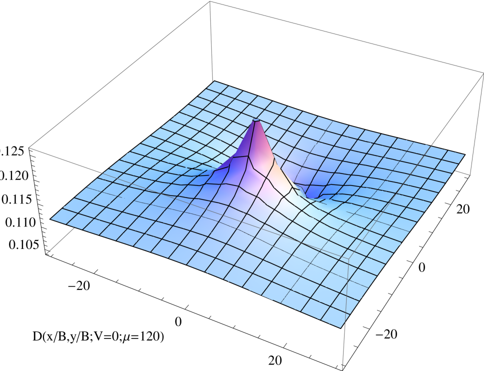
Figure 2: The tunneling density of states for $n=0$ , $\frac{dI}{dV}\propto D^{(n=0)}(\frac{x}{B^{(2)}},\frac{y}{B^{(2)}};\mu=120mV)$. The right corner represents the intersection of the $x$ coordinate which runs from $30$ (right corner) to $-30$ and the $y$ coordinate which runs from $-30$ (right corner) to $30$ in units of the Burger vector.

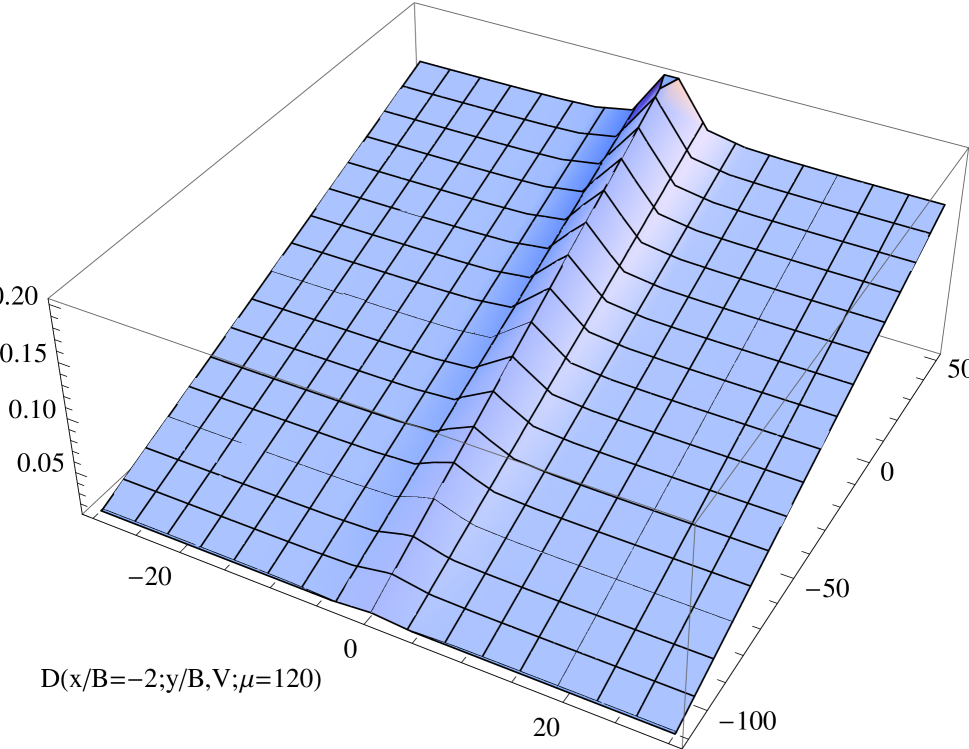
Figure 3: The tunneling density of states for $n=0$ as a function of $y$ and $V$ $\frac{dI}{dV}\propto D^{(n=0)}(\frac{x}{B^{(2)}}=-2,\frac{y}{B^{(2)}};\mu=120mV)$. The voltage range is $-120\leq V\leq 50$ and the $y$ coordinate is in the range $-30\leq\frac{y}{B^{(2)}}\leq 30$.

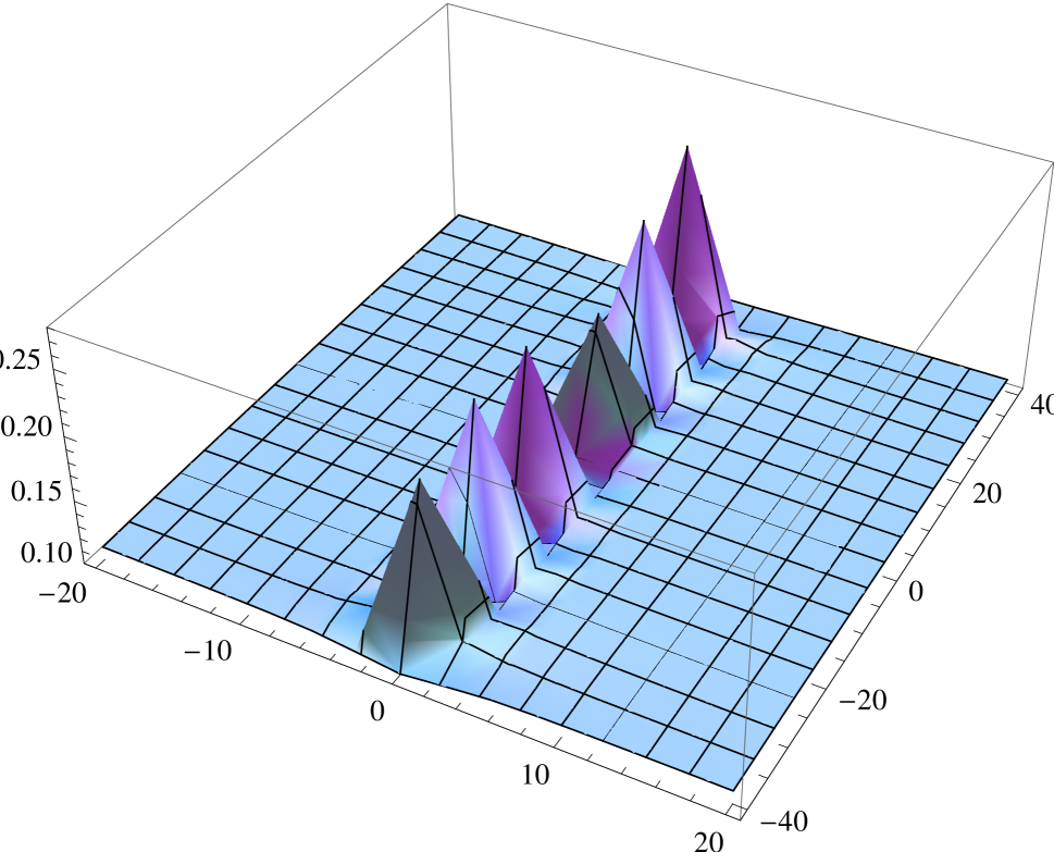
Figure 4: Many Dislocations - with the core of the dislocations at $[x_{w},y=0]$ , $w=1,2...2M$; The maximum of the tunneling density of states is confined along $y=0$. The coordinates of the tunneling density of states are restricted to : $-40\leq\frac{x}{B^{(2)}}\leq 40$ and $-20\leq\frac{y}{B^{(2)}}\leq 20$.

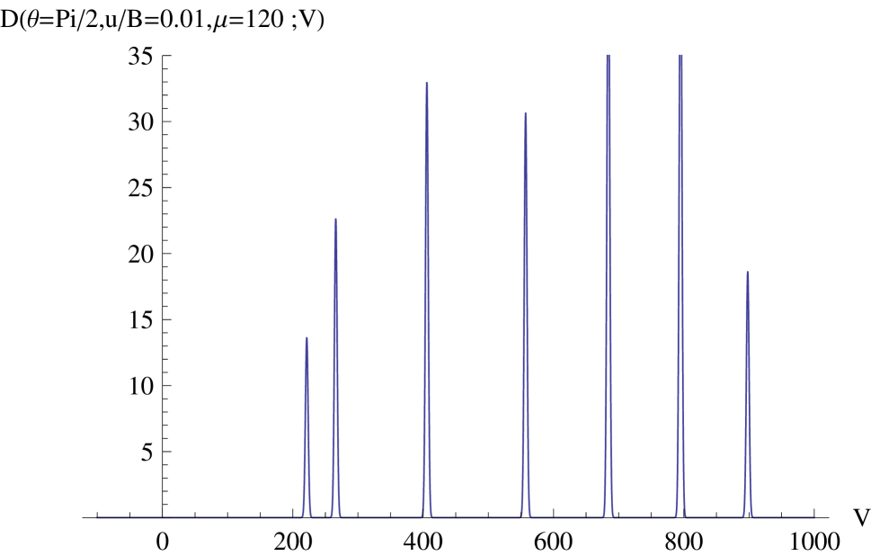
Figure 5: The discrete tunneling density of states for $n=1$, as a function of the voltage $V$ $D^{(n=1)}(V;\theta=\frac{\pi}{2},\frac{u}{B^{(2)}},\mu=120mV)$

Figure 6: The tunneling density of states as a function of $\theta$ $D^{(n=1)}(\theta;\frac{u}{B^{(2)}}=0.01,V=280mV,\mu=120mV)$

Figure 7: The tunneling density of states as a function of $\theta$ and $u$ at a fixed voltage $V=280mV$ $D^{(n=1)}(\theta,\frac{u}{B^{(2)}};V=280mV,\mu=120mV)$

References

(1)M.Konig et al.,Science 318,766 (2007)
(2) B.A.Volkov and O.A. Pankratov, JETP LETT. vol.42,179(1985)
(3) M.F.L.Gotelman, K.Jansen and D.B. Kaplan ”‘Chern-Simons Currents and Chiral Fermions on the Lattice ”‘ Phys.Lett.B301,219(1993).
(4) Michael Creutz and Ivan Horwath ”‘Surface States and Chiral Symmetry On The Lattice”’ Phys.Rev.50,2297(1994)
(5) C.L. Kane and E.J. Mele Phys.Rev. Lett. 95 226801 (2005)
(6) C.L. Kane and E.J. Mele ,‘Phys.Rev.Lett. 95,146802(2005).
(7) H.Zhang et al. nature physics 5,438,(2009).
(8)D. Schmeltzer, “Topological Insulators-transport in curved space”
, arXiv:1012.5871 and Advances in Condensed Matter and Materials Research ,volume 10 Editors:Hans Geelvinck and Sjaak Reyst ,chapter 9, pages 379-403(2011).
(9) J.E.Moore and L.Balents, cond-mat/0607314
(10) Andrew M.Essin and J.E.More, cond-mat/0705.0172.
(11) Xiao-Liang Qi, Taylor L.Hughes and Shou-Cheng Zhang , Phys.Rev.B78,195424(2008)
(12) Xiao-Liang Qi and Shou-Cheng Zhang cond-mat/1008.2026
(13) Andreas P. Schnyder, Shinsei Ryu, Akira Furusaki, Andreas W.W. Ludwig
cond-mat/0803.2786.
(14) M.Z.Hasan and C.L. Kane, cond-mat/1002.3895
(15) Ying Ran et.al , Nature Physics vol5,298 (2009)
(16) Chao-Xing Liu et al, Physical Review B 82 045122 (2010 ”‘
(17) S.Young et al. ”‘Theoretical Investigation Of The Topological Phase Of Under Mechanical Strain”’cond-mat/1106.5556
(18) O.A.Tretiakov et al Cond.Mat/1007.2966 .
(19) F.de Juan,A.Cortijo and M.A.H.Vozmediano, Phys.rev.B 76 165409(2007).
(20) A.Cortijo and M.H.A. Vozmediano, Nuclear Physics B 763[FS](2007) 293-308.
(21)F.Guinea, Baruch Horowitz, P.Le Doussal Solid State Communications 149,1140-1143 (2009)
(22)F.Guinea,Baruch Horovitz, and P.Le Doussal Phys.Rev.B 77,205421(2008)
(23) C.Kittel , Introduction to Solid State Physics ,eight edition 2005 John Willey and Sons,Inc. see pages and .
(24) M.Nakahara ”‘Geometry,Topology And Physics ”‘ Taylor Francis Press 2003.
(25) R.Jackiw and J.R. Schrieffer,Nuclear Physics B190,253-265,(1981)
(26) H.Kleinert ”‘Multivalued Fields in Condensed Mattewr ,Electromagnetism, and Gravitation”’ World Scientific (2008) pages 348-350.
(27) Z.F.Ezawa,”’Quantum Hall effects”’ World Scientific (2008).
(28) B.Andrea Bernevig Taylor L.Hughes, and Shou-Cheng Zhang cond-mat/061139.
(29) C. Wu,B. A. Bernevig and Shou-Cheng Zhang Phys.Rev.Lett. 96 106401 (2006).