Electrodynamics effects in $3+1$ dimensions induced by interactions in Topological Insulators

Abstract

We compute the optical response of an interacting topological insulator in three space dimensions. The interactions are induced by a chiral charge density wave and the interacting system is invariant under an arbitrary chiral transformation. We show that the chiral phase is gauged away from the action. For the case that the bands are inverted, the arbitrary phase of the Fujikawa integration measure is fixed by the charge density wave. We find that the magnetoelectric response which is generated by the integration measure breaks the time reversal symmetry. At strong interactions the time reversal is restored and the magnetoelectric effect is equivalent to the one obtained in topological insulators in four space dimensions without interaction. This effect can be observed by measuring the Faraday rotation as a function of an external stress.

I. Introduction

Insulators with spin-orbit interactions can give rise to either regular insulators or to topological insulators ($TI$). The low energy excitations of the insulators $Bi_{2}Se_{3}$ and $Bi_{2}Te_{3}$ can be approximated by a two-band model with spin-orbit interactions which respect the time reversal symmetry. One finds that when bands at the $\Gamma$ point are inverted the system is a $TI$ according to the classification of the second Chern number Nakahara or band invariants introduced in ref. Kane . One of the possible experimental evidence came from the Faraday effect, when light passes from a medium with $\theta=0$ (normal insulator) to a medium with $\theta\neq 0$ a rotation of the polarization is expected. Since time reversal symmetry is not broken the rotation must correspond to a topological angle $\theta=\pm\pi$ Wilczek ; Zhangaxion ; Zhangnew . One of the experimental difficulty arises from the fact that the experiments are performed in three space dimensions and the second Chern topological invariant exists in four space dimensions.

A formal solution to this problem was given in Zhangaxion ; Zhangnew ; ZhangField which suggested to use dimensional reduction. One performs the computations in four space dimensions and then compactifies one of the coordinates to a small circle. Other solutions based on a macroscopic polarization on the surface of the sample have been proposed ortiz ; Vanderbilt . An adiabatic approach to the polarization has been given in Niu for the second Chern number. The relation between the topological angle $\theta$ and quantization has been discussed in Franzaxion . Only recently the effect of interactions on $TI$ has been considered Haijun ; Stern . In particular, the question of charge density wave instability on the surface of $TI$ has been investigated in ref. Stern . The effect of an applied magnetic field on the surface of a topological insulator gives rise to a simple relation between the Faraday and Kerr rotations MacDonald .

The main purpose of this paper is to present a derivation for the optical response (magnetoelectric effect) of $TI$ in three space dimensions. We obtain this result using bond interactions and chiral currents for insulators with inverted bands. The interactions give rise to an effective action which is controlled by a bond order parameter. The action of the model with integration measure is invariant under an arbitrary chiral transformation Fujikawa . The saddle point and the fluctuations of the bond effective action fix the coefficient of the chiral transformation. As a result one obtains an electromagnetic action which breaks the time reversal symmetry. The coefficient of the electromagnetic term is determined by integration (governed by the saddle point) which fixes the topological angle $\theta$. Experimentally the topological angle is controlled by the coupling constants and external perturbations such as stress Young . The value of $\theta$ determines the Faraday rotation between two regions: the first region consists of an interacting $TI$ and the second region represents a non-interacting insulator. The value of $\theta$ in turn is determined by the integration over the bond order parameter. At particular values of $\theta=\pm\pi$, time reversal symmetry is restored and the system is a $TI$. For $\theta=0$ we have a regular insulator.

The contents of the paper are as follows: In Sec. II we introduce the model for the $TI$ in the presence of a bond interaction which, with the help of the Hubbard-Stratonovich transformation, is represented as a chiral charge density wave field $\varphi(\vec{r})$. Section III represents the central part of this paper, where we include the external electromagnetic field $\vec{A}^{ext}$ in the action. We perform a chiral transformation $e^{i\lambda(\vec{r})\gamma^{5}}$ for an arbitrary field $\lambda(\vec{r})$. Since the partition function is invariant under this transformation, the action and the integration measure are modified. The integration measure generates the term $\lambda(\vec{r})\vec{E}\cdot\vec{B}$ which breaks the time reversal symmetry. The fermionic action $S$ contains a modified bond order parameter which depends on the field $\lambda(\vec{r})$. The value of $\lambda(\vec{r})$ can be fixed by demanding that the transformed bond order parameter vanishes. As a result, the term $\lambda(\vec{r})\vec{E}\cdot\vec{B}$ becomes a function of $\lambda(\varphi(\vec{r}))$. We perform a saddle point integration over the bond order parameter and obtain the electromagnetic response function $\theta(\frac{e^{2}}{2\pi h})\vec{E}\cdot\vec{B}$ (where $\theta$ is a function of the fluctuation fields around the saddle point). Section IV contains our main conclusions.

II. Topological Insulator in three space dimensions

We will compute the optical response of the $TI$ materials $Bi_{2}Se_{3}$ and $Bi_{2}Te_{3}$. The low energy bands consist of four projected states, the conduction and valence states $|P1^{+}_{-},\pm\frac{1}{2}\rangle$ and $|P2^{+}_{-},\pm\frac{1}{2}\rangle$ near the Fermi surface at the $\Gamma$ point Wei ; Chao ; XingLiu . Due to the strong spin-orbit coupling the level $|P1^{+}_{-},\pm\frac{1}{2}\rangle$ is pushed down while $|P2^{+}_{-},\pm\frac{1}{2}\rangle$ is pushed up resulting in a band inversion. Using the notation $|orbital=\tau=1\rangle\otimes|spin=\sigma=\uparrow,\downarrow\rangle\equiv|P1^{+}_{-},\pm\frac{1}{2}\rangle$ and $|orbital=\tau=2\rangle\otimes|spin=\sigma=\uparrow,\downarrow\rangle\equiv|P2^{+}_{-},\pm\frac{1}{2}\rangle$ we obtain the effective Hamiltonian $\hat{h}^{3d}$ at the $\Gamma$ point: $\hat{h}^{3d}=k_{2}(\sigma^{1}\otimes\tau^{1})-k_{1}(\sigma^{2}\otimes\tau^{1})+\eta k_{3}(\sigma^{3}\otimes\tau^{1})+M(\vec{k})(I\otimes\tau^{3})$, where $M(\vec{k})-Bk^{2}$ determines whether the insulator is trivial or topological. For $\frac{M(0)}{B}>0$ we have a $TI$ (an insulator with an inverted gap) and a regular insulator for $\frac{M(0)}{B}<0$ Kane ; Zhangnew . The band anisotropy in the $z$ direction is given by $\eta\ll 1$. Due to Nielsen-Ninomiya theorem the total number of Dirac points must be even. The other Dirac points are not observed since the Hamiltonian is linearized around the $\Gamma$ point and contains additional non-relativistic terms Advances . The eigenvalues in the vecinity of the $\Gamma$ point are given by $E(\vec{k})=\pm\sqrt{k^{2}_{1}+k^{2}_{2}+\eta^{2}k^{2}_{3}+M(\vec{k})^{2}}$. We extend the model (with a single Dirac point) to a torus and demand the momentum periodicity $-\pi\leq k_{1}\leq\pi$ ,$-\pi\leq k_{2}\leq\pi$ ,$-\pi\leq k_{3}\leq\pi$. It is convenient to perform a unitary transformation $U=(e^{i\frac{\pi}{4}\sigma^{3}}\otimes I)$:

$$h^{3d}=U^{-1}\hat{h}^{3d}U=k_{1}\alpha^{1}+k_{2}\alpha^{2}+\eta k_{3}\alpha^{3}+M(\vec{k})\beta,$$ (1)

where the matrices $\alpha$ and $\beta$ are given by: $\alpha^{i}=(\sigma^{i}\otimes\tau_{1})$, $i=1,2,3$ and $\beta=(I\otimes\tau_{3})$.

Next we include the bond interactions in three space dimensions. We consider a particular type of bond interaction $H_{int.}$ in three space dimensions which we describe using the four component spinor $\Psi(\vec{r})=[\Psi_{\tau=1}(\vec{r}),\Psi_{\tau=2}(\vec{r})]^{T}$, where $\Psi_{\tau}(\vec{r})$ is a two component spinor with $\sigma=\uparrow,\downarrow$, $\Psi_{\tau}(\vec{r})=[\Psi_{\tau,\uparrow}(\vec{r}),\Psi_{\tau,\downarrow}(\vec{r})]^{T}$ and $n_{\tau,\sigma}(\vec{r})=\Psi^{\dagger}_{\tau,\sigma}(\vec{r})\Psi_{\tau,\sigma}(\vec{r})$ represents the fermion number for the orbital $\tau$ and spin $\sigma$.

$$H_{int}=\frac{-U_{eff}}{2}\int d^{3}r$$

$$\left[\sum_{\sigma=\uparrow,\downarrow}\left(\Psi^{\dagger}_{\tau=1,\sigma}(\vec{r})\Psi_{\tau=2,\sigma}(\vec{r})-\Psi^{\dagger}_{\tau=2,\sigma}(\vec{r})\Psi_{\tau=1,\sigma}(\vec{r})\right)\right]^{\dagger}\left[\sum_{\sigma=\uparrow,\downarrow}\left(\Psi^{\dagger}_{\tau=1,\sigma}(\vec{r})\Psi_{\tau=2,\sigma}(\vec{r})-\Psi^{\dagger}_{\tau=2,\sigma}(\vec{r})\Psi_{\tau=1,\sigma}(\vec{r})\right)\right]$$

$$=\frac{U_{eff}}{2}\int d^{3}r\left[\sum_{\sigma=\uparrow,\downarrow}\Psi^{\dagger}_{\tau=1,\sigma}(\vec{r})\Psi_{\tau=2,\sigma}(\vec{r})-\sum_{\sigma=\uparrow,\downarrow}\Psi^{\dagger}_{\tau=2,\sigma}(\vec{r})\Psi_{\tau=1,\sigma}(\vec{r})\right]^{2}$$

$$=\frac{-U_{eff}}{2}\int d^{3}r[\Psi^{\dagger}(\vec{r})(I\otimes\tau^{2})\Psi^{\dagger}(\vec{r})]^{2},$$ (2)

where $U_{eff}>0$. The action for the three dimensional $TI$ $h^{3d}$ with the interaction $H_{int}$ is given by:

$$S=\int_{-\infty}^{\infty}dt\int d^{3}r\Big{[}\Psi^{\dagger}(\vec{r},t)\Big{[}i\partial_{t}+i\alpha^{1}\partial_{1}+i\alpha^{2}\partial_{2}+i\eta\alpha^{3}\partial_{3}$$

$$-\beta(M(0)-B\sum_{l=1,2}\partial^{2}_{l})\Big{]}\Psi(\vec{r},t)+\frac{U_{eff}}{2}(\Psi^{\dagger}(\vec{r})(I\otimes\tau^{2})\Psi^{\dagger}(\vec{r}))^{2}\Big{]}.$$ (3)

Using the Hubbard-Stratonovich transformation we replace the interaction term by a chiral density wave field $\varphi(\vec{r},t)$. The interaction corresponds to a charge density wave order which acts between the bands (orbitals). Such an interaction can be induced by phonons which couple between the orbitals and can be enhanced by external stress. Thus,

$$S=\int_{-\infty}^{\infty}dt\int d^{3}r\Big{[}\bar{\Psi}(\vec{r},t)\Big{[}i\gamma^{0}\partial_{t}+i\gamma^{1}\partial_{1}+i\gamma^{2}\partial_{2}+i\eta\gamma^{3}\partial_{3}$$

$$-(M(0)-B\sum_{l=1,2}\partial^{2}_{l})+i\gamma^{5}\sqrt{U_{eff}}\varphi(\vec{r},t)\Big{]}\Psi(\vec{r},t)\Big{]}-\frac{1}{2}\int_{-\infty}^{\infty}dt\int d^{3}r\varphi^{2}(\vec{r},t).$$

In Eq. (4) we have replaced $\Psi^{\dagger}(\vec{r},t)\rightarrow\bar{\Psi}(\vec{r},t)=\Psi^{\dagger}(\vec{r},t)\gamma^{0}$ and introduced the anti-commuting gamma matrices:

$$\gamma^{0}=\beta\equiv(I\otimes\tau^{3}),\hskip 7.22743pt\gamma^{i}=\beta\alpha^{i}\equiv(\sigma^{i}\otimes i\tau^{2}),~{}~{}i=1,2,3,\hskip 7.22743pt\gamma^{5}=(I\otimes\tau^{1}).$$ (5)

From Hubbard-Stratonovich transformation we observe that the interaction corresponds to a charge density wave order which acts between the bands (orbitals). Such an interaction can be induced by phonons which couple between the orbitals and can be enhanced by an external stress. The justification for the chiral coupling $i\gamma^{5}\sqrt{U_{eff}}\varphi(\vec{r},t)$ must take into consideration the Nielsen-Ninomiya theorem about the even number of Dirac modes which are absent in our Hamiltonian. The second Dirac point is pushed away by the non-relativistic terms. In ref. Advances we have introduced a lattice model which recovers, in the continuum limit, our model. The model consists of $H_{lattice}=H_{so}+H_{M}+H_{nrel}$, $H_{so}=iz_{so}\sum_{i=1,2,3}\Psi^{\dagger}(\vec{r})(\sigma^{i}\otimes\tau)\Psi(\vec{r}+\vec{a}_{i})+H.C.$ ( $\vec{a}_{i}$ are the Bravais lattice vectors ). $H_{so}$ has an even number of Dirac points. When the mass term $H_{M}=M(0)\Psi^{\dagger}(\vec{r})(I\otimes\tau_{1})\Psi(\vec{r})$ is included a mass gap is opened. The non-relativistic term $H_{nrel}=-t\sum_{i=1,2,3}\Psi^{\dagger}(\vec{r})(I\otimes\tau)\Psi(\vec{r}+\vec{a}_{i})$ removes the Dirac points which are not at the $\Gamma$ point.

The mass term arises due to the momentum difference between the right and left mover fermions. This can be understood in the following way: we expand each orbital using the even number of Dirac points $\vec{K}_{r}$ ,$r=1,2..even$, $\Psi_{\tau=1}(\vec{r})=\sum_{r=1,...,even}\psi_{\tau=1,r}(\vec{r})e^{i\vec{\vec{K}}_{r}\cdot\vec{r}}$ and $\Psi_{\tau=2}(\vec{r})=\sum_{r=1,...,even}\psi_{\tau=2,r}(\vec{r})e^{i\vec{\vec{K}}_{r}\cdot\vec{r}}$. The unit cell of the crystals consists of five atoms (two $Bi$ and three $Se$). The $Bi$ atoms are displaced by a vector $\vec{s}<\vec{a}_{i}$ relative to the $Se$ atom ($\vec{a}_{i}$ are the Bravais lattice vectors). We have two equivalent Se atoms and two equivalent Bi atoms and a lattice distortion can remove this degeneracy. Using a projection method we approximate the problem to two spinors which correspond to the two Fermi points ($\vec{K}_{r=-}$ and $\vec{K}_{r=+}$): $\Psi(\vec{r})=[\Psi_{\tau=1}(\vec{r}),\Psi_{\tau=2}(\vec{r})]^{T}\approx[\psi_{\tau=1,r=+}(\vec{r})e^{i\vec{\vec{K}}_{r=+}\cdot\vec{r}},\psi_{\tau=2,r=-}(\vec{r})e^{i\vec{\vec{K}}_{r=-}\cdot\vec{r}}]$. As a result the mass term carries a momentum $\vec{Q}=\vec{K}_{r=+}-\vec{K}_{r=-}$. The $H_{M}$ Hamiltonian is modified: $H_{M}\approx M(\vec{r})\Psi^{\dagger}_{\tau=1}(\vec{r})\Psi_{\tau=2}(\vec{r})+M^{*}(\vec{r})\Psi^{*}_{\tau=2}(\vec{r})\Psi_{\tau=1}(\vec{r})\approx M(0)\Psi^{\dagger}(\vec{r})(I\otimes\tau_{1})\Psi(\vec{r})++i\sqrt{U_{eff}}\varphi(\vec{r})\Psi^{\dagger}(\vec{r})(I\otimes\tau_{2})\Psi(\vec{r})$, where $M(0)\equiv M(\vec{r})+M^{*}(\vec{r})$ and $\sqrt{U_{eff}}\varphi(\vec{r})\equiv M(\vec{r})-M^{*}(\vec{r})$.

The transformation from the Dirac fields $\Psi_{\tau=1}(\vec{r})$,$\Psi_{\tau=2}(\vec{r})$ to the Weyl fields $\Psi_{R}(\vec{r})$,$\Psi_{L}(\vec{r})$ allows to make contact with the one dimensional systems such as organic materials Schrieffer : $\Psi_{\tau=1}(\vec{r})=\frac{1}{\sqrt{2}}[\Psi_{R}(\vec{r})+\Psi_{L}(\vec{r})]$, $\Psi_{\tau=2}(\vec{r})=\frac{1}{\sqrt{2}}[\Psi_{R}(\vec{r})-\Psi_{L}(\vec{r})].$ It has been shown that in one dimension such terms give rise to solitons and the electronic excitations carry fractional charges Schrieffer ; Rebi ; Goldstone which is not the case for three dimensions. The interacting model in the chiral form is given by:

$$M(0)(\Psi^{\dagger}_{\tau=1}(\vec{r})\Psi_{\tau=1}(\vec{r})-\Psi^{\dagger}_{\tau=2}(\vec{r})\Psi_{\tau=2}(\vec{r}))+i\varphi(\vec{r})(\Psi^{\dagger}_{\tau=1}(\vec{r})\Psi_{\tau=2}(\vec{r})-\Psi^{\dagger}_{\tau=2}(\vec{r})\Psi_{\tau=1}(\vec{r}))$$

$$=M(0)[\Psi^{\dagger}_{R}(\vec{r})\Psi_{L}(\vec{r})+\Psi^{\dagger}_{L}(\vec{r})\Psi_{R}(\vec{r})]+i\varphi(\vec{r})[\Psi^{\dagger}_{R}(\vec{r})\Psi_{L}(\vec{r})-\Psi^{\dagger}_{L}(\vec{r})\Psi_{R}(\vec{r})].$$ (6)

We observe that the combination $M(0)+i\gamma^{5}\sqrt{U_{eff}}\varphi(\vec{r})$ is chiral invariant (in the chiral notation the combination $M(0)\pm i\sqrt{U_{eff}}\varphi(\vec{r})$ is chiral invariant). When we perform the chiral transformation the combination $M(0)+i\gamma^{5}\sqrt{U_{eff}}\varphi(\vec{r})$ is transformed $(M(0)+i\gamma^{5}\sqrt{U_{eff}}\varphi(\vec{r}))\rightarrow(M^{\prime}(0)+i\gamma^{5}\sqrt{U_{eff}}\varphi^{\prime}(\vec{r}))=e^{-i\lambda\gamma^{5}}[M(0)+i\gamma^{5}\sqrt{U_{eff}}\varphi(\vec{r})]e^{i\lambda\gamma^{5}}$.

Integration over the fermion field $Z=\int[D\varphi][D\bar{\Psi}][D\Psi]e^{iS}=\int[D\varphi]e^{iS_{eff}[\varphi(\vec{r})]}$ generates an effective action $S_{eff}[\varphi(\vec{r})]$ which shows that the combination $M^{2}+U_{eff}\varphi^{2}(\vec{r})$ is invariant. (For the one dimensional case this symmetry implies the existence of domain walls and solitons Goldstone .) The term $i\gamma^{5}\sqrt{U_{eff.}}\varphi(\vec{r},t)$ breaks the time reversal symmetry. The Hamiltonian with the interactions takes the form: $h^{(3d-int)}[\vec{k},\sqrt{U_{eff.}}\varphi(\vec{r})]=k_{1}\gamma^{1}+k_{2}\gamma^{2}+\eta k_{3}\gamma^{3}+M(\vec{k})+i\gamma^{5}\sqrt{U_{eff.}}\varphi(\vec{r})$. Time reversal invariance demands that $T^{-1}h^{(3d-int)}[\vec{k},\sqrt{U_{eff.}}\varphi(\vec{r})]T=h^{(3d-int)}[-\vec{k},\sqrt{U_{eff.}}\varphi(\vec{r})]$ where $T=i(\sigma_{2}\otimes I)\textbf{K}$ is the time reversal operator. Performing the time reversal transformation we find that the term $i\gamma^{5}\sqrt{U_{eff.}}\varphi(\vec{r},t)$ indeed breaks the time reversal symmetry: $T^{-1}h^{(3d-int)}[\vec{k},\sqrt{U_{eff.}}\varphi(\vec{r})]T=h^{(3d-int)}[-\vec{k},-\sqrt{U_{eff.}}\varphi(\vec{r})]\neq h^{(3d-int)}[-\vec{k},\sqrt{U_{eff.}}\varphi(\vec{r})]$.

The computation of the magnetoelectric response is obtained by expanding the action in terms of the external electromagnetic fields. This calculation is done in the following way: we restrict the chiral transformation such that the transformed coefficient $i\gamma^{5}$ is absent in the action. This means that the contribution from the action will not contain terms which violate the time reversal symmetry. The electromagnetic part which violates the time reversal symmetry is due to the path integration measure Fujikawa . The chiral transformation which eliminates the term $i\gamma^{5}$ from the action, restricts the chiral transformation to $2\lambda=\pm\pi$. Consequently, the chiral transformation is restricted to a $Z_{2}$ transformation. The $Z_{2}$ symmetry is broken spontaneously, and we can expand the effective action around the broken symmetry state. For this case we have zero Goldstone modes but no solitons.

III. Computation of the magnetoelectric response for a $TI$ in three space dimensions

In this section we will compute the electromagnetic response for the interacting ‘inverted’ insulator $\frac{M(0)}{B}>0$ in three space dimensions. Since the interaction model breaks the time reversal symmetry we obtain a magnetoelectric response. For the strong coupling case the proportionality coefficient is given by $\pm\pi$. As a result we obtain that the magnetoelectric response does not violate the time reversal symmetry. We obtain the result using the chiral charge density wave field $i\gamma^{5}\sqrt{U_{eff}}\varphi(\vec{r})$ and and chiral transformation $e^{i\gamma^{5}\lambda(\vec{r})}$ with the arbitrary field $\lambda(\vec{r})$. We perform the chiral transformation using the existing results given in the literature Fujikawa ; Nakahara ; Ludwig ; Burkov . In our problem the saddle point with respect to the field $i\sqrt{U_{eff}}\varphi(\vec{r})\gamma^{5}$ allows us to fix the value of the field $\lambda(\vec{r})\equiv\lambda(\varphi(\vec{r}))$. Consequently, the saddle point field fixes the coefficient of the magnetoelectric response $\vec{E}^{ext.}\cdot\vec{B}^{ext}$ and determines the topological angle $\theta$. In order to compute the electromagnetic response we will include in the action $S$ the external electromagnetic field, $\vec{A}^{ext}(\vec{r},t)=[A^{ext}_{1}(\vec{r}),A^{ext}_{2}(\vec{r}),A^{ext}_{3}(\vec{r},t)]$:

$$S[\bar{\Psi},\Psi,\varphi]=\int_{-\infty}^{\infty}dt\int d^{3}r\Big{[}\bar{\Psi}(\vec{r},t)[i\gamma^{0}(\partial_{t}-eA^{ext}_{0})+i\gamma^{1}(\partial_{1}-eA^{ext}_{1})+i\gamma^{2}(\partial_{2}-eA^{ext}_{2})$$

$$+i\eta\bar{\gamma}^{3}(\partial_{3}-eA^{ext}_{3})$$

$$-\left(M(0)-B\sum_{l}\partial^{2}_{l}\right)+i\gamma^{5}\sqrt{U_{eff}}\varphi(\vec{r},t)]\Psi(\vec{r},t)\Big{]}-\frac{1}{2}\int_{-\infty}^{\infty}dt\int d^{3}r\varphi^{2}(\vec{r},t).$$ (7)

Next we perform the chiral transformation:

$$\bar{\Psi}(\vec{r},t)\rightarrow\hat{\bar{\Psi}}(\vec{r},t)=e^{i\lambda(\vec{r},t)\gamma^{5}}\bar{\Psi}(\vec{r},t),\hskip 7.22743pt\Psi(\vec{r},t)\rightarrow\hat{\Psi}(\vec{r},t)=e^{i\lambda(\vec{r},t)\gamma^{5}}\Psi(\vec{r},t)$$ (8)

The action transforms like:

$$S[\bar{\Psi},\Psi,\varphi;M(0)]\rightarrow S[\hat{\bar{\Psi}},\hat{\Psi},\varphi;M(0]$$

$$=S[\bar{\Psi},\Psi,\varphi;M(0)]+\int dt\int d^{3}\Big{[}\lambda(\vec{r})[\partial_{1}(\bar{\Psi}(\vec{r},t)\gamma^{1}\gamma^{5}\Psi(\vec{r},t)+\partial_{2}(\bar{\Psi}(\vec{r},t)\gamma^{2}\gamma^{5}\Psi(\vec{r},t))$$

$$+\eta\partial_{3}(\bar{\Psi}(\vec{r},t)\gamma^{3}\gamma^{5}\Psi(\vec{r},t))]-[M(0)(\cos(2\lambda(\vec{r},t))-1)+\sqrt{U_{eff}}\varphi(\vec{r},t)\sin(2\lambda(\vec{r})]\bar{\Psi}(\vec{r},t)\Psi(\vec{r},t)$$

$$+i[\sqrt{U_{eff}}\varphi(\vec{r},t)(\cos(2\lambda(\vec{r},t)-1)-M(0)\sin(2\lambda(\vec{r},t))]\bar{\Psi}(\vec{r},t)\gamma^{5}\Psi(\vec{r},t)+B\bar{\Psi}(\vec{r},t)\gamma^{5}\sum_{l}\partial^{2}_{l}\Psi(\vec{r},t)\Big{]},$$

and the partition function obeys the equality:

$$Z=\int[D\varphi][D\bar{\Psi}][D\Psi]e^{iS[\bar{\Psi},\Psi,\varphi]}=\int[D\varphi][D\hat{\bar{\Psi}}][D\hat{\Psi}]e^{iS[\hat{\bar{\Psi}},\hat{\Psi},\varphi]}.$$ (10)

Using the fact that the measure $[D\bar{\Psi}][D\Psi]$ is not invariant under the chiral transformation Fujikawa we obtain the result in units where $h=c=1$:

$$[D\hat{\bar{\Psi}}][D\hat{\Psi}]=[D\bar{\Psi}][D\Psi]e^{i\frac{e^{2}}{2\pi}\int_{-\infty}^{\infty}dt\int d^{3}r[\lambda(\vec{r})(\vec{E}^{ext}(\vec{r})\cdot\vec{B}^{ext}(\vec{r},t))]}.$$ (11)

Since the field is arbitrary we can choose this field such that the coefficient of $\gamma^{5}$ vanishes. As a result the action obtained is time reversal invariant and the leading electromagnetic contribution is due only to the measure. The term $\gamma^{5}\sqrt{U_{eff}}\varphi(\vec{r})$ becomes $\gamma^{5}[\sqrt{U_{eff}}\varphi(\vec{r},t)\cos(2\lambda(\vec{r},t))-M(0)\sin(2\lambda(\vec{r},)]$ for a particular choice of $\lambda(\vec{r})$ and the coefficient of $\gamma^{5}$ vanishes,

$$\tan(2\lambda(\vec{r},t))=\frac{\sqrt{U_{eff}}\varphi(\vec{r},t)}{M(0)}.$$ (12)

For this value of $\lambda(\vec{r},t)$ we can absorb the interaction field $\varphi(\vec{r},t)$ into a new mass $\hat{M}(\varphi^{2}(\vec{r},t))$ (the term which describes the inverted bands):

$$M(0)\rightarrow M(0)\sqrt{1+\frac{U_{eff}\varphi^{2}}{M^{2}(0)}}\equiv M(\varphi^{2}(\vec{r},t)).$$ (13)

The partition function can be written as:

$$Z=\int[D\varphi][D\bar{\Psi}][D\Psi]e^{iS[\bar{\Psi},\Psi,M(\varphi^{2}(\vec{r},t))),0]}e^{i\int_{-\infty}^{\infty}dt\int d^{3}r(-\frac{\sqrt{U_{eff.}}}{(M(0))}\vec{\partial}\varphi(\vec{r},t)\cdot[\bar{\Psi}(\vec{r},t)\vec{\gamma}\gamma^{5}\Psi(\vec{r},t)]}$$

$$\times e^{i\frac{e^{2}}{2\pi}\int dt\int d^{3}r\Big{[}\frac{1}{2}ArcTan[\frac{\sqrt{U_{eff.}}}{(M(0))}\varphi(\vec{r},t)]\vec{E}^{ext}(\vec{r})\cdot\vec{B}^{ext}(\vec{r})\Big{]}}e^{i\int_{-\infty}^{\infty}dt\int d^{3}r\frac{-\varphi^{2}(\vec{r},t)}{2}},$$ (14)

where

$$S[\bar{\Psi},\Psi,M(\varphi^{2}(\vec{r}))),0]=$$

$$\int_{-\infty}^{\infty}dt\int d^{3}r\Big{[}\bar{\Psi}(\vec{r},t)[i\gamma^{0}(\partial_{t}+ieA^{ext}_{0})+i\hbar\gamma^{1}(\partial_{1}+ieA^{ext}_{1})+i\gamma^{2}(\partial_{2}+ieA^{ext}_{2})$$

$$+i\eta\gamma^{3}(\partial_{3}+ieA^{ext}_{3})-(M(\varphi^{2}(\vec{r},t))-B\sum_{l}\partial^{2}_{l})+i\gamma^{5}(0)]\Psi(\vec{r},t))\Big{]}$$

$$\equiv\int_{-\infty}^{\infty}dt\int d^{3}r\Big{[}\bar{\Psi}(\vec{r},t)[i\gamma^{0}(\partial_{t}+ieA^{ext}_{0})-h^{3D-eff.}(\vec{k},M(\varphi^{2}(\vec{r},t)))]\Psi(\vec{r},t))\Big{]}.$$ (15)

The action $S[\bar{\Psi},\Psi,M(\varphi^{2}(\vec{r},t)),0]$ does not break the time reversal symmetry, therefore the integration of the fermions generates only regular Maxwell terms. We perform the integration with respect to the fermions and compute the effective potential for zero electromagnetic fields.

$$\int[D\bar{\Psi}][D\Psi]e^{iS[\bar{\Psi},\Psi,M(\varphi^{2}(\vec{r},t)),0]}e^{i\int_{-\infty}^{\infty}dt\int d^{3}r\frac{-\varphi^{2}(\vec{r},t)}{2}}=$$

$$e^{-i\int_{-\frac{T}{2}}^{\frac{T}{2}}dt\int d^{3}r[\frac{\varphi^{2}(\vec{r},t)}{2}+iLnDet\Big{[}i\gamma^{0}\partial_{t}-h^{3D-eff.}(\vec{k},M(\varphi^{2}(\vec{r},t))]\Big{]}}\approx e^{-i\int_{-\frac{T}{2}}^{\frac{T}{2}}\int d^{3}r\Big{[}W^{(3D-eff.)}[\varphi(\vec{r})]\Big{]}}$$

$$W^{(3D-eff.)}[\varphi(\vec{r})]=\frac{\varphi^{2}}{2}+i\int_{-\infty}^{\infty}\frac{d\omega}{\pi}\int_{0}^{\Lambda}\frac{d^{3}k}{(2\pi)^{3}}Ln\Big{[}\omega^{2}-[k^{2}_{1}+k^{2}_{2}+\eta^{2}k^{2}_{3}+(M(\varphi^{2},t)-Bk^{2})^{2}]+i\epsilon\Big{]}.$$

We introduce the ultraviolet cut-off $\Lambda$ Shankar and replace the effective gap $M(0)\equiv\Lambda\hat{M}(0)$ and the coupling constant $\frac{1}{U_{eff}}\equiv\hat{g}_{eff.}\Lambda^{d-1}$. The field $\varphi(\vec{r},t)$ is replaced with $\hat{\Phi}(\vec{r},t)$, defined through the relation: $\sqrt{U_{eff.}}\varphi(\vec{r},t)=\Phi(\vec{r})\equiv(\frac{\Phi(\vec{r},t)}{M(0)})M(0)$, $\frac{\Phi(\vec{r},t)}{M(0)}\equiv\hat{\Phi}(\vec{r},t)$.

The effective potential in Eq. $(16)$ is a function of the sign of the parameter $B$. The number of zero eigenvalues in the energy spectrum $E(\vec{k})=\pm\sqrt{[k^{2}_{1}+k^{2}_{2}+\eta^{2}k^{2}_{3}+(\hat{M}(\varphi^{2})-Bk^{2})^{2}]}$ determines if the system is a regular insulator or a $TI$. For a positive mass $M(0)$ and $B<0$ the eigenvalues have no zero energy states. Computing the effective potential for this case ($B<0$) shows that $W^{(3D-eff)}[\varphi(\vec{r})]$ has only a single minimum for $\varphi(\vec{r})=0$. Therefore the magnetoelectric effect is absent and the system is a regular insulator in agreement with the literature. For the case $B>0$ , $E(\vec{k})$ has zero energy states. The effective potential $W^{(3D-eff)}[\varphi(\vec{r})]$ for this case has non-zero saddle points giving rise to a magnetoelectric effect and the system is a $TI$ in agreement with the condition $\frac{M(0)}{B}>0$.

For the remaining part we restrict our calculation to the $TI$ case $\frac{M(0)}{B}>0$. We compute the effective potential for $d=3$ , $0<B\Lambda^{2}\ll 1$ and $\eta\rightarrow 0$:

$$W^{(3d-eff)}[\hat{\Phi}(\vec{r})]=\frac{1}{2}\hat{g}_{eff.}(\hat{M}(0))\Lambda^{4}\hat{\Phi}^{2}(\vec{r})-\frac{2}{(2\pi)^{3}}\int_{0}^{\Lambda}d^{2}k_{\bot}\int_{-\Lambda}^{\Lambda}dk_{3}$$

$$\Big{[}\sqrt{k^{2}_{1}+k^{2}_{2}+\eta^{2}k^{2}_{3}+\Lambda^{2}\hat{M}^{2}(0)(1+\hat{\Phi}^{2}(\vec{r}))}-\sqrt{k^{2}_{1}+k^{2}_{2}+\eta^{2}k^{2}_{3}}\Big{]}$$

$$\frac{W^{(3d-eff)}[\hat{\Phi}(\vec{r})]}{\Lambda^{4}}\approx\frac{1}{2}\hat{g}_{eff.}\hat{M}^{2}(0)\hat{\Phi}^{2}(\vec{r})-\frac{1}{6\pi^{2}}\Big{[}[1+\hat{M}^{2}(0)(1+\hat{\Phi}^{2}(\vec{r}))]^{\frac{3}{2}}$$

$$-[1+[\hat{M}^{2}(0)(1+\hat{\Phi}^{2}(\vec{r}))]^{\frac{3}{2}}\Big{]}.$$ (17)

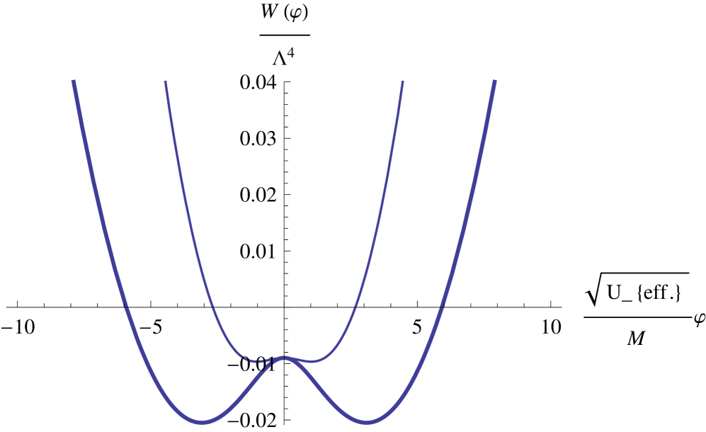
Figure 1: The effective potential $W(\sqrt{U_{eff}}\varphi)$ for $(\hat{M}(0))=0.75$. The lower graph (the thicker line) represents the effective potential for $\hat{g}_{eff}\equiv\frac{1}{\hat{U}_{eff}}=0.01$. For this case the saddle point corresponds to $\sqrt{U_{eff}}\varphi=\varphi^{*}=\pm\pi$. The upper graph represents the effective potential for a weaker coupling $\hat{g}_{eff}\equiv\frac{1}{\hat{U}_{eff}}=0.02$. As a result we find that $\sqrt{U_{eff}}\varphi\approx\pm 1$.

In Fig. 1 we plot the effective potential $\frac{W^{(3d-eff)}[\hat{\Phi}(\vec{r},t)]}{\Lambda^{4}}$ for the inverted gap $\frac{M(0)}{B}>0$. Varying the values of the coupling constant $U_{eff}$ (controlled by the pressure) $\varphi$ decreases below $\pi$. The value $\varphi<\pi$ corresponds to a phase with a broken time reversal symmetry. At strong coupling the order parameter takes the values $\varphi=\varphi^{*}=\pm\pi$ and the time reversal symmetry is restored.

Using the effective potential $W^{(3D-eff)}[\varphi(\vec{r},t)]=W^{(3D-eff)}[\hat{\Phi}(\vec{r},t)]$ we compute the electromagnetic response:

$$Z=\int[D\varphi]e^{-iW^{(3D-eff)}[\varphi(\vec{r},t)]}e^{i\frac{e^{2}}{2\pi}\int dt\int d^{3}r[\frac{1}{2}ArcTan[\frac{\sqrt{U_{eff}}}{(M(0)}\varphi(\vec{r},t)](\vec{E}^{ext}(\vec{r})\cdot\vec{B}^{ext}(\vec{r}))]}$$

$$\approx e^{i\theta(\frac{e^{2}}{2\pi})\int_{-\infty}^{\infty}dt\int d^{3}r\vec{E}^{ext}(\vec{r})\cdot\vec{B}^{ext}(\vec{r})}\equiv e^{i\delta S^{(3)}_{eff}}.$$ (18)

The results in the last equation have been obtained with the help of the saddle point integration. The effective potential $W^{3D-eff}[\varphi(\vec{r},t)]$ has a saddle point $\pm\sqrt{U_{eff}}\varphi\equiv\Phi\neq 0$. We perform the integration of the field $\varphi(\vec{r})$ expanding the action around the saddle point $\Phi\neq 0$, $\Phi(\vec{r})=\Phi+\delta\Phi(\vec{r},t)$. The fluctuation field $\delta\Phi(\vec{r},t)$ corresponds to the zero frequency Goldstone mode. The Goldstone mode can create a domain wall for the case when the interactions are restricted to half space.

In summary, we find that when $\sqrt{U_{eff}}\langle\varphi(\vec{r},t)\rangle=\Phi\neq 0$ the time reversal symmetry is broken and the effective action is given by Eq. $(18)$. In the limit of strong interaction the expectation value can attain the value $\sqrt{U_{eff}}\langle\varphi(\vec{r})\rangle=\Phi^{*}=\pm\pi$. At these values of $\Phi^{*}=\theta=\pm\pi$ and the time reversal symmetry is restored.

In the last part of this paper we want to comment about the possibility of solitons for three dimensional crystals. This can be achieved by replacing the scalar field $\varphi(\vec{r})$ by a vector field $\vec{\varphi}(\vec{r})\cdot\vec{S}$ which couples through the Pauli matrix $\vec{S}$ to two Fermi points like in graphene , $\hat{\Omega}(\vec{r},t)=[\bar{\Psi}^{F1}(\vec{r},t),\bar{\Psi}^{F2}(\vec{r},t)]$ where $F1$ and $F2$ are the two Fermi points. As a result the effective action is modified,

$$\hat{S}=\int_{-\infty}^{\infty}dt\int d^{3}r\Big{[}\hat{\Omega}(\vec{r},t)[i\gamma^{0}\partial_{t}+i\gamma^{1}\partial_{1}+i\gamma^{2}\partial_{2}+i\eta\gamma^{3}\partial_{3}$$

$$-(M(0)-B\sum_{l=1,2}\partial^{2}_{l})+i\gamma^{5}\sqrt{U_{eff}}\vec{\varphi}(\vec{r},t)\cdot\vec{S}]\Omega(\vec{r},t)\Big{]}-\frac{1}{2}\int_{-\infty}^{\infty}dt\int d^{3}r\vec{\varphi}^{2}(\vec{r},t)$$

According to Goldstone this action can support monopole fields which are the analog of stable kinks in higher dimensions. In the condensed matter the monopole fields are similar to dislocations Schmeltzer .

Next we consider the experimental realization. For practical applications we will assume that the interaction term $\sqrt{U_{eff}}\varphi(\vec{r},t)\gamma^{5}$ is restricted to half space. Such a restriction will always guarantee that the topological angle is not zero. In order to confirm the topological behavior we have to measure the nonlinear response given by the Faraday and Kerr rotations. The electrodynamics in the presence of the new term $\theta\vec{E}\cdot\vec{B}$ has been studied in Hehl ; Karch . Using this theory one can compute the relation between the Faraday rotation (transmission) and Kerr rotation (reflection) that is relevant to the topological angle $\theta$. We predict that the Faraday rotation together with the Kerr rotation will be sensitive to external perturbations such as pressure. Therefore, by changing the pressure we can induce a change in the rotation and identify the topological angle $\theta=\pm\pi$. According to the sensitivity reported (10 $nrad$) in ref. Kapitulnick the experiments suggested there seem to be achievable. The authors in ref .Kapitulnick use a reflection mirror to distinguish between a Faraday rotation which breaks the time reversal symmetry and the one which does not. (For a system which breaks the time reversal symmetry one finds that due to the reflection the Faraday rotation is twice the original one, and for a system which respects the time reversal symmetry the angle of rotation after the reflection is zero.)

According to refs. Senthil ; Nagaosa the magnetoelectric effect can give rise to fractional statistics or magnetic texture on the surface of the $TI$. Therefore transport measurements on the surface of the $TI$ can differentiate between the different predictions which correspond to different topological angles.

IV. Conclusions

We have computed the magnetoelectric effect in the presence of interactions for a $TI$ in three space dimensions. We find that for a particular type of bond interaction which is described as a chiral charge density wave we obtain an electromagnetic response which breaks the time reversal symmetry. We find the magnetoelectric response $\theta(\frac{e^{2}}{2\pi})\int_{-\infty}^{\infty}dt\int d^{3}r[\vec{E}^{ext}(\vec{r})\cdot\vec{B}^{ext}(\vec{r})]$ which depends on the topological angle $\theta$. At strong couplings $\theta=\pm\pi$, the time reversal symmetry is restored and we obtain that the electromagnetic response of the three dimensional $TI$ with interactions is equivalent to the non-interacting $TI$ in four space dimensions. The saddle point is sensitive to an external $stress$, therefore this theory can be tested by measuring the Faraday and Kerr rotations of a $TI$ crystal under variable hydrostatic stress.

References

(1) M. Nakahara, Geometry, Topology And Physics (Taylor and Francis, Philadelphia, 2003).
(2) L. Fu and C. L. Kane, Phys. Rev. B 76, 045302 (2007).
(3) F. Wilczek, Phys. Rev. Lett. 58, 1799 (1987).
(4) Y. Lan, S. Wan, and S.-C. Zhang, Phys. Rev. B 83, 205109 (2011).
(6) X.-L. Qi, T. L. Hughes, and S.-C. Zhang, Phys. Rev. B 78, 195424 (2008).
(7) G. Ortiz and R. L. Martin, Phys. Rev. Rev. B 49, 14202 (1994).
(8) A. M. Essin and J. E. Moore, Phys. Rev. B 76, 165307 (2007); A. M. Essin, J. E. Moore, and D. Vanderbilt, Phys. Rev. Lett. 102, 146805 (2009); A. M. Essin, A. M. Turner, J. E. Moore, and D. Vanderbilt, Phys. Rev. B 81, 205104 (2010).
(9) D. Xiao, J. Shi, D. P. Clougherty, and Q. Xiu, Phys. Rev. Lett. 102, 087602 (2009).
(10) M. M. Vazifeh and M. Franz, Phys. Rev. B 82, 233103 (2010).
(11) X. Zhang, H. Zhang, J. Wang, C. Felser, and S.-C. Zhang, Science 235, 1464 (2012).
(12) Y. Baum and A. Stern, cond-mat 1208.2576v1.
(13) W.-K. Tse and A. H. MacDonald, Phys. Rev. B 84, 205327 (2011).
(14) K. Fujikawa, Phys. Rev. Lett. 42, 1195 (1979).
(15) S. M. Young, S. Chowdhuri, E. J. Walter, E. J. Mele, C. L. Kane, and A. M. Rappe, Phys. Rev. B 84, 085106 (2011).
(16) W. Zhang, R. Yu, H.-J. Zhang , X. Dai, and Z. Fang, New J. Phys. 12, 065013 (2010).
(17) C. X. Liu, H. J. Zhang, B. Yan, X. L. Qi, T. Frauenheim, X. Dai, Z. Fang, and S.-C. Zhang, Phys. Rev. B 81, 041307R (2010).
(18) C. X. Liu, X. L. Qi, H. J. Zhang, X. Dai, Z. Fang, and S.-C.Zhang, Phys. Rev. B 82, 045122 (2010).
(19) Advances in Condensed Matter and Material Research Volume 10, pp. 379-402, Eds. Hans Geelvinck and Sjaak Reynst (Nova Publishers, Hauppauge, NY, 2011).
(20)W. P. Su, J. R. Schrieffer, and Heeger, Phys. Rev. Lett.42, 1698 (1979).
(21) J. Goldstone and F. Wilczek, Phys. Rev. Lett. 47, 986 (1981).
(22)R. Jackiw and C. Rebi, Phys. Rev. D 13, 3398 (1976).
(23) S. Ryu, J. E. Moore, and A. W. W. Ludwig, Phys. Rev. B 85, 045104 (2012).
(24) A.A. Zyuzin and A.A. Burkov, cond-mat 1206.1868 (2012).
(25) R. Shankar, Rev. Mod. Phys. 66, 129 (1994).
(26) D. Schmeltzer, New J. Phys. 14, 1637 (2012).
(27)Y. N. Obukhov and F. W. Hehl, Phys. Lett. A 34, 357 (2005).
(28)A. Karch, Phys. Rev. Lett. 17, 171601 (2009).
(29) A. Kapitulnick , J. Xiar, E. Schermm, and A. Palevski, New J. Phys. 11, 055060 (2009).
(30) B. Swingle, M. Barkeshil, J. M. McGreevy, and T. Senthill, Phys. Rev. B 83,195139 (2011).
(31) K. Nomura and N. Nagaosa, Phys. Rev. B 82, 161401R (2010).