Exploring Gauge-Invariant Vacuum Wave Functionals for Yang-Mills Theory

Abstract:

We study gauge-invariant approximations to the Yang-Mills vacuum wave functional in which asymptotic freedom and a detailed description of the infrared dynamics are encoded through squeezed core states. After variationally optimizing these trial functionals, dimensional transmutation, gluon condensation and a dynamical mass gap of the expected magnitude emerge transparently. The dispersion properties of the soft gauge modes are modified by higher-gradient interactions and suggest a negative differential color resistance of the Yang-Mills vacuum. Casting the soft-mode dynamics into the form of an effective action for gauge-invariant collective fields, furthermore, allows to identify novel infrared degrees of freedom. The latter are gauge-invariant saddle-point fields which summarize dominant and universal contributions from various gauge-field orbits to all amplitudes. Their analysis provides new insights into how the vacuum gluon fields generate gauge-invariant excitations. Examples include a dynamical size stabilization mechanism for instantons and merons, a gauge-invariant representation of their effects as well as a new physical interpretation for Faddeev-Niemi knots.

1 Introduction

The Hamiltonian formulation of Yang-Mills (YM) theory in the Schrödinger picture, although not particularly efficient in the perturbative domain, offers considerable benefits when addressing nonperturbative issues. Among its attractive features are the explicit representation of the vacuum state which invokes quantum mechanical intuition [1], the ability to treat genuine real-time problems (including non-equilibrium processes) as well as the transparent description of topological effects [2]. In particular, however, it makes gauge theories accessible to a variational treatment [1, 3], i.e. to one of the few approximation schemes currently available for strongly coupled quantum field theories.

Variational calculations in Yang-Mills theories are often performed in a fixed gauge, most notably in Coulomb gauge [4]. In the following we will report on our complementary explorations [5] of a manifestly gauge-invariant formulation of the variational problem [6]. This framework renders fundamental infrared (IR) physics, including dimensional transmutation and the generation of a mass gap, particularly transparent. Moreover, it preserves the full topological structure of the gauge group. The latter is particularly relevant since topological properties are likely robust enough to survive limitations of the restricted trial functional basis which keeps the approach analytically manageable. Another attractive feature of the gauge-invariant formulation is that the infrared dynamics can be re-expressed in terms of gauge-invariant collective fields which subsume contributions from whole gauge-field orbit families. After performing an IR improved variational analysis [5], we will make use of this feature to identify gauge-invariant and universal IR degrees of freedom of the gauge dynamics [7]. More details can be found in Refs. [5, 7].

2 Gauge-invariant vacuum wave functionals

Starting from an approximate and hence typically gauge-dependent “core” functional $\psi_{0}\left[\vec{A}\right]$ of the static gauge fields (i.e. of half of the canonical variables), we impose gauge invariance by averaging over the gauge group. The result is a trial vacuum wave functional (VWF) of the form

$$\Psi_{0}\left[\vec{A}\right]=\sum_{Q\in Z}e^{iQ\theta}\int D\mu\left[U^{\left(Q\right)}\right]\psi_{0}\left[\vec{A}^{U^{\left(Q\right)}}\right]=:\int DU\psi_{0}\left[\vec{A}^{U}\right]$$ (1)

where $d\mu$ is the Haar measure of the SU$\left(N_{c}\right)$ gauge group, $Q$ the topological (homotopy) charge of the group element $U^{\left(Q\right)}$, and $\theta$ the vacuum angle. Since the vacuum wave functional is nodeless [1], one may write $\psi_{0}\left[\vec{A}\right]=\mathcal{N}^{-1}\exp\left(-\Phi\left[\vec{A}\right]\right)$ and expand the real functional $\Phi$ into a power series. The constant term is absorbed into $\mathcal{N}$ and the term linear in $A$ is generally discarded (coherent gluon vacuum states are known to be unstable [8]).

The next term is quadratic in $A$ and plays several crucial roles. First, it removes the ambiguity in $\Psi_{0}$ [9] due to the invariance of the Haar measure in Eq. (1) under group transformations. Furthermore, this term can incorporate asymptotic freedom and thus render the VWF exact in the ultraviolet. Finally, and from the practical perspective most importantly, functionals resulting from a quadratic term can be integrated over $A$ analytically. Hence one generally truncates the series for $\Phi$ after the quadratic term, which leads to the “squeezed” core functional

$$\psi_{0}^{\left(G\right)}\left[\vec{A}\right]=\frac{1}{\mathcal{N}_{G}}\exp\left[-\frac{1}{2}\text{ }\int d^{3}x\int d^{3}yA_{i}^{a}\left(\vec{x}\right)G_{ij}^{-1ab}\left(\vec{x}-\vec{y}\right)A_{j}^{b}\left(\vec{y}\right)\right]$$ (2)

with the normalization factor $\mathcal{N}_{G}^{-1}=\left[\det\left(G/2\right)\right]^{-1/4}$ and a real “covariance” $G^{-1}$.

2.1 Gluon dispersion: asymptotic freedom and IR generality

We now have to specify the properties of the function $G^{-1}$ in the trial functional family (2). Translational invariance was already anticipated in Eq. (2). We will further restrict ourselves to a purely transverse covariance with the Fourier transform [6]

$$G_{ij}^{-1,ab}\left(k\right)=\delta_{ij}\delta^{ab}G^{-1}\left(k\right)$$ (3)

(cf. Ref. [5] for a discussion of this choice and Refs. [10, 11] for the impact of longitudinal contributions). The normalizability of physical wave functionals then demands $G^{-1}\left(k\right)>0$ and further ensures vacuum stability and a positive energy spectrum. In order to implement the correct UV behavior, we factorize the core functionals (2) as $\psi_{0}^{\left(G\right)}\left[\vec{A}\right]=\psi_{0}^{\left(G_{<}\right)}\left[\vec{A}_{<}\right]\psi_{0}^{\left(G_{>}\right)}\left[\vec{A}_{>}\right]$ by splitting the $\vec{k}$ integration domain in their exponentials into soft/hard momentum regions with $\left|\vec{k}\right|\gtrless\mu$. The separation scale $\mu$ will be determined below. Asymptotic freedom requires $G$ to approach the non-interacting, massless static vector propagator $G_{0}\left(k\right)=1/k$ for $k\rightarrow\infty$. As long as $\mu\gg\Lambda_{\text{YM}}$ (where $\Lambda_{\text{YM}}$ is the Yang-Mills scale) perturbative hard-mode corrections remain small, which allows us to approximate

$$G_{>}^{-1}\left(k\right)=G_{0}^{-1}\left(k\right)=k.$$ (4)

The unknown IR covariance $G_{<}^{-1}\left(k\right)$, on the other hand, will be determined variationally. In Ref. [6] the minimal one-parameter trial function $G_{<,\text{KK}}^{-1}\left(k\right)=\mu$ was adopted. We have implemented a far more comprehensive parametrization [7], based on the under reasonable analyticity assumptions general and controlled gradient expansion

$$G_{<}^{-1}\left(\vec{x}-\vec{y}\right)=m_{g}\left[1+c_{1}\frac{\partial_{x}^{2}}{\mu^{2}}+c_{2}\left(\frac{\partial_{x}^{2}}{\mu^{2}}\right)^{2}+c_{3}\left(\frac{\partial_{x}^{2}}{\mu^{2}}\right)^{3}+...\right]\delta_{<}^{3}\left(\vec{x}-\vec{y}\right).$$ (5)

Eq. (5) can be efficiently truncated to maintain an analytically manageable trial basis for the soft-mode physics. Besides $\mu$, the variational parameter space now contains the IR gluon mass $m_{g}>0$ and a few low-momentum constants $c_{i}$ which characterize dispersive gluon properties in the vacuum. The regularized delta function $\delta_{<}^{3}\left(\vec{x}-\vec{y}\right):=\int d^{3}k/\left(2\pi\right)^{3}\theta\left(\mu^{2}-\vec{k}^{2}\right)e^{i\vec{k}\left(\vec{x}-\vec{y}\right)}$ encodes the slow variation $\left\|\partial A_{<}\right\|/\left\|A_{<}\right\|\leq\mu$ of the soft modes and ensures that the higher-order terms in Eq. (5) are parametrically suppressed.

As a consequence of $G^{-1}\left(k\right)>0$, the low-momentum constants are subject to the bounds $c_{1}<1,$ $c_{2}>-1$, etc. (for $m_{g}>0$). Requiring continuity of $G^{-1}\left(k\right)$ at the matching point $k=\mu$, furthermore, fixes $m_{g}$ as a function of the other variational parameters. When truncating to $c_{i\geq 2}=0$, for example, one has

$$m_{g}\left(\mu,c_{1}\right)=\frac{\mu}{1-c_{1}}.$$ (6)

Note that the requirement of a non-negative IR gluon mass restricts the $c_{1}$ domain to $c_{1}<1$, in agreement with the above bound from $G^{-1}\left(k\right)>0$. The VWF (1) together with the core functional (2) and the covariance (4), (5) (possibly with perturbative corrections) appears to be the “richest” gauge-invariant trial functional family whose matrix elements can be calculated analytically by currently available techniques.

3 Variational analysis

One the basis of the trial functional family (1) discussed above, the variational analysis amounts to minimizing the expectation value

$$\left\langle\mathcal{H}\left(A,E\right)\right\rangle=\frac{\int D\vec{A}\Psi_{0}^{\ast}\left[\vec{A}\right]\mathcal{H}\left(\vec{A}^{a},\vec{E}^{a}\right)\Psi_{0}\left[\vec{A}\right]}{\int D\vec{A}\Psi_{0}^{\ast}\left[\vec{A}\right]\Psi_{0}\left[\vec{A}\right]}$$ (7)

of the Yang-Mills Hamiltonian density

$$\mathcal{H}=\frac{1}{2}\left(E_{i}^{a}E_{i}^{a}+B_{i}^{a}B_{i}^{a}\right)$$ (8)

(in temporal gauge, with $\vec{E}^{a}=i\delta/\delta\vec{A}^{a}$) with respect to the parameters appearing in $G^{-1}$. After inserting the wave functional (1) into Eq. (7) and interchanging the order of integration over fields and group elements, the gauge invariance of the $\vec{A}$ integral allows to factor out a gauge group volume. Eq. (7) can thus be rewritten as

$$\left\langle\mathcal{H}\left(A,E\right)\right\rangle=\frac{\int DU\int D\vec{A}\psi_{0}\left[\vec{A}^{U}\right]\mathcal{H}\left(\vec{A}^{a},\frac{i\delta}{\delta\vec{A}^{a}}\right)\psi_{0}\left[\vec{A}\right]}{\int DU\int D\vec{A}\psi_{0}\left[\vec{A}^{U}\right]\psi_{0}\left[\vec{A}\right]}$$ (9)

(where $DU$ is the functional SU$\left(N_{c}\right)$ measure as defined in Eq. (1)). After evaluating the functional derivatives contained in $\mathcal{H}$, the Gaussian integration over $A$ can be performed exactly, resulting in

$$\left\langle\mathcal{H}\right\rangle=\frac{\int DU\left\langle\left\langle\left\langle\mathcal{H}\right\rangle\right\rangle\right\rangle\exp\left\{-\Gamma_{b}\left[U\right]\right\}}{\int DU\exp\left\{-\Gamma_{b}\left[U\right]\right\}}$$ (10)

where we introduced the notation

$$\left\langle\left\langle\left\langle\vec{A}...\vec{A}...\vec{E}...\vec{E}\right\rangle\right\rangle\right\rangle\exp\left\{-\Gamma_{b}\left[U\right]\right\}\equiv\int D\vec{A}\psi_{0}\left[\vec{A}^{U}\right]\vec{A}...\vec{A}...\frac{i\delta}{\delta\vec{A}}...\frac{i\delta}{\delta\vec{A}}\psi_{0}\left[\vec{A}\right]$$ (11)

for matrix elements between $U$-rotated and unrotated core VWFs. The above expression defines, in particular, the effective bare action $\Gamma_{b}\left[U\right]=-\ln\int D\vec{A}\,\ \psi_{0}^{\ast}\left[\vec{A}^{U}\right]\psi_{0}\left[\vec{A}\right]$ which describes dynamical correlations generated by the gauge projection. This action gathers all those gauge-field contributions to the generating functional whose approximate vacua $\psi_{0}$ at $t=\pm\infty$ differ by a relative gauge orientation $U$. Hence the gauge-invariant “variable” $U$ represents the contributions from all such gluon field orbits to the vacuum overlap. Explicitly, one finds [5]

$$\Gamma_{b}\left[U\right]=\frac{1}{2g_{\text{b}}^{2}}\int d^{3}x\int d^{3}yL_{i}^{a}\left(\vec{x}\right)\mathcal{D}^{ab}\left(\vec{x}-\vec{y}\right)L_{i}^{b}\left(\vec{y}\right)$$ (12)

with $L_{i}=U^{\dagger}\partial_{i}U=:L_{i}^{a}\lambda^{a}/\left(2i\right)$ and $\mathcal{D}^{ab}=\left[\left(G+G^{U}\right)^{-1}\right]^{ab}\simeq\frac{1}{2}G^{-1}\delta^{ab}+...$ where $G^{U}=G^{ab}\left(\vec{x}-\vec{y}\right)$ $U^{\dagger}\left(\vec{x}\right)\left(\lambda^{a}/2\right)U\left(\vec{x}\right)\otimes U\left(\vec{y}\right)\left(\lambda^{b}/2\right)U^{\dagger}\left(\vec{y}\right)$.

After splitting $U\left(\vec{x}\right)=U_{<}\left(\vec{x}\right)U_{>}\left(\vec{x}\right)$ with $U_{>}\left(\vec{x}\right)=\exp\left(-ig\phi^{a}\left(\vec{x}\right)\lambda^{a}/2\right)$ into hard- and soft-mode contributions and integrating over the hard modes $\phi^{a}$ perturbatively [6], furthermore, one arrives at

$$\left\langle\mathcal{H}\right\rangle=\frac{\int DU_{<}\int D\phi\left\langle\left\langle\left\langle\mathcal{H}\right\rangle\right\rangle\right\rangle\exp\left\{-\Gamma_{b}\left[\phi,U_{<}\right]\right\}}{\int DU_{<}\int D\phi\exp\left\{-\Gamma_{b}\left[\phi,U_{<}\right]\right\}}.$$ (13)

With the additional definition

$$\left\langle\left\langle\mathcal{O}\right\rangle\right\rangle\exp\left\{-\Gamma_{<}\left[U_{<}\right]\right\}:=\int D\phi\left\langle\left\langle\left\langle\mathcal{O}\right\rangle\right\rangle\right\rangle\exp\left\{-\Gamma_{b}\left[\phi,U_{<}\right]\right\},$$ (14)

which contains the effective soft-mode action

$$\Gamma_{<}\left[U_{<}\right]:=-\ln\int D\phi\exp\left\{-\Gamma_{b}\left[\phi,U_{<}\right]\right\}$$ (15)

(i.e. the RG evolved bare action (12)), we can finally rewrite the matrix element (7) solely in terms of the $U_{<}$ field dynamics, i.e.

$$\left\langle\mathcal{H}\right\rangle=\frac{\int DU_{<}\left\langle\left\langle\mathcal{H}\right\rangle\right\rangle\exp\left\{-\Gamma_{<}\left[U_{<}\right]\right\}}{\int DU_{<}\exp\left\{-\Gamma_{<}\left[U_{<}\right]\right\}}.$$ (16)

Since the “reduced” (i.e., fixed $U_{<}$) matrix element $\left\langle\left\langle\mathcal{H}\right\rangle\right\rangle$ is a nonlocal functional of the soft modes $U_{<}$, the evaluation of Eq. (16) amounts to calculating (equal-time) soft-mode correlation functions [5].

3.1 Vacuum phases

In integrals over the $U_{<}$ fields (such as those in Eq. (16)) the unitarity constraint $U_{<}^{\dagger}U_{<}=1$ can be resolved by inserting a delta functional which is then written as an additional integral over a hermitean auxilary field $\Sigma$. In Eq. (16) the integration over the then unconstrained $U_{<}$ becomes Gaussian and can be done analytically. In the mean-field approximation, the expression for $\left\langle\left\langle\mathcal{H}\right\rangle\right\rangle$ is then evaluated at the saddle point $\bar{\Sigma}=:\left(\mu\bar{\xi}\right)^{2}$ of the $\Sigma$ integral, i.e. at the minimal-action solution of the gap equation

$$\left\langle U_{<,AB}^{\dagger}\left(\vec{x}\right)U_{<,BC}\left(\vec{x}\right)\right\rangle=\delta_{AC}$$ (17)

which reintroduces unitarity in the mean. After adopting the one-loop Yang-Mills coupling $\gamma\left(\mu\right)=g_{\text{YM}}^{2}\left(\mu\right)N_{c}/\pi^{2}\overset{N_{c}=3}{=}24/\left(11\ln\mu/\Lambda_{\text{YM}}\right)$, the solutions $\bar{\xi}$ of Eq. (17) depend on two variational parameters, the RG scale $\mu\geq 0$ and $c_{1}<1$. The critical line $\mu_{c}\left(c_{1}\right)$, i.e. the parameter subspace where the (dis-)order parameter $\bar{\xi}\left(\mu_{c}\left(c_{1}\right),c_{1}\right)$ vanishes and the phase transition takes place, can be found analytically as the combination of the two curves

$$\frac{\mu_{c,1,2}\left(c_{1}\right)}{\Lambda_{\text{YM}}}=\exp\left[\frac{48}{11}\frac{\left(1-c_{1}\right)\left[1-\tilde{\imath}\left(c_{1}\right)\right]\left[1+\left(1-c_{1}\right)\tilde{\imath}\left(c_{1}\right)\right]}{\left(1-c_{1}\right)\tilde{\imath}\left(c_{1}\right)\pm\sqrt{5\tilde{\imath}^{2}\left(c_{1}\right)\left(1-c_{1}\right)^{2}-4\left(1-c_{1}\right)\left[1-c_{1}\tilde{\imath}\left(c_{1}\right)\right]}}\right]$$ (18)

($\tilde{\imath}\left(c_{1}\right):=\mathrm{arctanh}\sqrt{c_{1}}/\sqrt{c_{1}}$). We plot this closed phase boundary in Fig. 1. It limits the parameter ranges to $0.5\lesssim\frac{\mu_{\text{c}}}{\Lambda_{\text{YM}}}\lesssim 8.86$ and $-0.48\lesssim c_{1}<1\$and thus prevents the minimal-energy solution $\bar{\xi}^{\ast}$ from attaining unacceptably large values of $\mu$ and $\left|c_{1}\right|$. Nonzero solutions of the gap equation exist only when the gauge coupling exceeds a critical value, i.e. for $g^{2}\left(\mu\right)>g_{\text{c}}^{2}\left(c_{1}\right),$ as expected on physical grounds. The (dis-)order parameter goes to zero continuously, furthermore, i.e. the disorder-order transition is of second order (which may be an artefact of the mean-field approximation [5]).

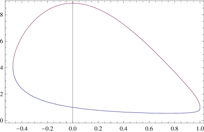
Figure 1: The vacuum phase diagram. Inside the plotted phase boundary $\mu_{c}\left(c_{1}\right)/\Lambda_{\text{YM}}$ the theory is in its strongly-coupled disordered phase. (The underlying approximations are reliable for $\mu\gtrsim 4\Lambda_{\text{YM}}$ and $c_{1}\in\left\{-0.5,0.5\right\}$).

3.2 Vacuum energy density

Working with the Poincaré-invariant trial states (1) and taking only one-loop corrections from the hard modes into acccount, it is sufficient to regularize Eq. (7) by a momentum cutoff $\Lambda_{\text{UV}}$ [6]. Separating the complete vacuum energy density $\varepsilon=E/V=\left\langle\mathcal{H}_{\text{YM}}\right\rangle$ into hard and soft contributions,

$$\varepsilon\left(\mu,c_{1},\zeta;\bar{\xi}\right)=\left\langle\mathcal{H}_{\text{YM}}\right\rangle=\varepsilon_{>}\left(\mu\right)+\varepsilon_{<}\left(\mu,c_{1},\zeta;\bar{\xi}\right),$$ (19)

($\zeta\equiv m_{g}/\mu$) the cutoff dependence resides solely in

$$\varepsilon_{>}\left(\mu\right)=\frac{N_{c}^{2}-1}{8\pi^{2}}\left(\Lambda_{\text{UV}}^{4}-\mu^{4}\right).$$ (20)

As expected, this is the (regularized) zero-point energy density of two transverse, massless vector modes in the adjoint representation of SU($N_{c}$) with energy $\omega\left(k\right)=k$. Simple normal-ordering thus subtracts the $\Lambda_{\text{UV}}$ dependent term. For $c_{i\geq 2}=0$ one then finds the total energy density $\bar{\varepsilon}\left(\mu,c_{1}\right):=$ $\varepsilon\left(\mu,c_{1},\zeta_{\text{ct}}\left(c_{1}\right);\bar{\xi}\left(\mu,c_{1}\right)\right)$ in the disordered phase as

$$\bar{\varepsilon}\left(\mu,c_{1}\right)= -\frac{N_{c}^{2}}{4\pi^{2}}\mu^{4}\left[\frac{4c_{1}^{3}+10c_{1}^{2}-50c_{1}+30}{30c_{1}^{2}\left(1-c_{1}\right)}-\frac{1-c_{1}}{c_{1}^{2}}\frac{\mathrm{arctanh}\sqrt{c_{1}}}{\sqrt{c_{1}}}\right.$$

$$+\left.\frac{\tilde{\imath}_{2}-2c_{1}\tilde{\imath}_{3}+c_{1}^{2}\tilde{\imath}_{4}+2\gamma c_{1}\left(1-c_{1}\right)\tilde{\imath}_{2}\left(\tilde{j}_{3}-2c_{1}\tilde{j}_{4}+c_{1}^{2}\tilde{j}_{5}\right)}{1-c_{1}}\right]$$ (21)

where the integrals $\tilde{\imath}_{n}\left(\xi,c_{1}\right),$ $\tilde{j}_{n}\left(\xi,c_{1}\right)$ are defined in Ref. [5] and evaluated at $\bar{\xi}\left(\mu,c_{1}\right)$. This energy density is plotted in Fig. 2.

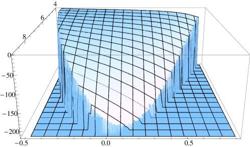
Figure 2: The energy density $\bar{\varepsilon}\left(\mu,c_{1}\right)$ of the vacuum field solution $\bar{\xi}\left(\mu,c_{1}\right)$ in the disordered phase. (The plot shows the parameter ranges $\mu\in\left\{4,9\right\}\Lambda_{\text{YM}}$ and $c_{1}\in\left\{-0.5,0.8\right\}.$) Note the minimum of the energy surface at $c_{1}\simeq 0.15$.

In the ordered phase, i.e. for $\mu\ggg\Lambda_{\text{YM}}$ where $g^{2}\left(\mu\right)\ll 1$, the energy density can be calculated perturbatively (in $g^{2}$). Since fluctuations $\varphi_{<}^{a}$ around $U_{<}\sim 1$ are small in this phase, one may approximate $U_{<}=\exp\left(ig\varphi_{<}^{a}\lambda^{a}\right)=1+ig\varphi_{<}^{a}\lambda^{a}+O\left(g^{2}\right).$ After adding the hard-mode contribution (20) and discarding the zero-point contribution, this results in

$$\varepsilon\left(\mu,c_{1}\right)=\frac{N_{c}^{2}-1}{4\pi^{2}}\mu^{4}\frac{1-c_{1}}{c_{1}^{2}}\left[-\frac{c_{1}^{3}+15c_{1}^{2}-50c_{1}+30}{30\left(1-c_{1}\right)^{2}}+\frac{\mathrm{arctanh}\sqrt{c_{1}}}{\sqrt{c_{1}}}\right].$$ (22)

It is reasonable to expect that this perturbative result remains qualitatively reliable down to the phase transition at $\mu_{c}$ [6]. The singularity of the energy density at $c_{1}\rightarrow 1$ encodes the vacuum instability for $c_{1}\geq 1$ and thus automatically ensures that the wave functional remains normalizable during the variational analysis.

The most important lesson of the above analysis is that $\varepsilon\left(\mu,c_{1}\right)$ increases monotonically with $\mu$ and $c_{1}$ (for $-2<c_{1}<1$) in the ordered phase while the energy density (21) in the strongly-coupled disordered phase monotonically decreases with $\mu$ and $c_{1}$, up to the phase transition. This indicates that the vacuum energy density becomes minimal at the phase boundary in the disordered phase, i.e. at $\bar{\xi}=0_{+}$ (where the number of massless particles becomes maximal [5]). The precise minimum, $\bar{\varepsilon}\left(\mu^{\ast},c_{1}^{\ast}\right)\simeq-210.59\Lambda_{\text{YM}}^{4},$ is reached at $c_{1}^{\ast}\simeq 0.15$ with $\mu^{\ast}=\mu_{c}\left(c_{1}^{\ast}\right)=8.61\Lambda_{\text{YM}}.$ These values justify the perturbative treatment of the hard modes and of the $4U$ contributions. The $c_{1}$ corrections reduce the vacuum energy density by about 11% and provide a rather substantial improvement of the wave functional.

3.3 Gluon condensate and quasigluon kinetic mass

At the physical parameter values, i.e. at the border of the disordered phase where the energy is minimal, the gluon condensate becomes

$$\left\langle F^{2}\right\rangle=-\frac{N_{c}^{2}-1}{\pi^{2}}\mu^{4}\left[\frac{7c_{1}^{3}-20\gamma^{\ast}c_{1}^{3}+15c_{1}^{2}+20\gamma^{\ast}c_{1}^{2}-50c_{1}+30}{30c_{1}^{2}\left(1-c_{1}\right)}-\left(\frac{1-c_{1}}{c_{1}^{2}}+\frac{2\gamma^{\ast}}{3}\right)\frac{\mathrm{arctanh}\sqrt{c_{1}}}{\sqrt{c_{1}}}\right]$$ (23)

($\gamma^{\ast}=g^{2}\left(\mu^{\ast}\right)N_{c}/\pi^{2}\simeq 1.012$). Numerically, this implies

$$\left\langle\frac{\alpha}{\pi}F^{2}\right\rangle=20.87\Lambda_{\text{YM}}^{4}\simeq 0.011\text{ GeV}^{4}$$ (24)

(for $\Lambda_{\text{YM}}\simeq 0.15$ GeV), i.e. an about 25% larger value than in the uncorrected $c_{1}=0$ case. The result (24) lies comfortably within the standard range $\left\langle\left(\alpha/\pi\right)F^{2}\right\rangle=0.0080-0.024$ GeV⁴ obtained from QCD sum rules [12].

Our finite and positive result for $c_{1}$ has further interesting consequences since it reshapes the composition and dispersion of the vacuum field population. Indeed, the attractive IR interactions generated by $c_{1}>0$ deplete the density of ultralong-wavelength $k\rightarrow 0$ modes and populate the $k\sim\mu$ modes more strongly. This is consistent with the expected average wavelength $\lambda\sim\Lambda_{\text{YM}}^{-1}$ of the vacuum fields. Since $G^{-1}\left(k\right)$ describes the dispersion relation $\omega\left(k\right)$ of “quasigluon” modes in the vacuum, furthermore, one may relate $c_{1}$ to the modulus of the dimensionless quasigluon group velocity $\vec{v}\left(\vec{k}\right)=\partial G_{<}^{-1}\left(\vec{k}\right)/\partial\vec{k}$ at $k=\mu$ [5],

$$\left|c_{1}\right|=\frac{v\left(\mu\right)}{v\left(\mu\right)+2}.$$ (25)

For $0>c_{1}>1$ (as in our case), furthermore, the “effective kinetic gluon mass” $\overline{m}_{\text{g}}$, which relates velocity and momentum as $\vec{k}=\overline{m}_{\text{g}}\vec{v}$, is negative. Hence $\vec{v}$ is opposite to the momentum, causing the “quasigluons” in the vacuum to decelerate when an external force is applied. (Such dispersions are encountered in several condensed-matter systems and are in stark contrast to the behavior of free gluons.) Hence quasigluons (with their small scattering amplitudes) may show a negative differential color resistance.

4 Infrared degrees of freedom

Our above representation of the vacuum dynamics in terms of the gauge-invariant low-energy fields $U_{<}$ provides the opportunity to search for specific $U_{<}$ which may play a particularly important or even dominant role in the generating functional (and hence universally in all low-energy amplitudes) [13]. If such fields exist, they can be regarded as universal infrared degrees of freedom (IRdofs). In contrast to other proposed IRdof candidates (e.g. classical gauge-field solutions like instantons [14], or monopole and vortex configurations), the IRdofs expressed in terms of $U_{<}$ are gauge invariant and contain crucial quantum effects (e.g. those which stabilize the instanton size, see below). From a practical perspective, these IRdofs will be useful as well since many technical problems encountered when dealing with gauge-dependent fields are avoided from the outset. Below we will show that large classes of such IRdofs indeed exist and review how their stability and topology emerges. We then construct important IRdof classes explicitly and discuss their properties and physical interpretation.

4.1 Gauge-invariant saddle point expansion

We start from the vacuum overlap matrix element, i.e. the functional integral

$$Z=\int DU_{<}\exp\left(-\Gamma\left[U_{<}\right]\right)$$ (26)

over the soft modes, with the action $\Gamma$ given by Eq. (15). (Sources can be included when needed.) A steepest descent approximation for $Z$ can be set up by expanding $U_{<}$ around the saddle point fields $\bar{U}_{i}\left(\vec{x}\right)$, i.e. the local minima of the soft-mode action (15) which solve

$$\left.\frac{\delta\Gamma\left[U_{<}\right]}{\delta U_{<}\left(\vec{x}\right)}\right|_{U_{<}=\bar{U}_{i}^{\left(Q\right)}}=0.$$ (27)

(Different topological charges (see below) are summarily denoted by $Q$ since the action is varied in each topological sector separately.) To leading order, the saddle point expansion for $Z$ is then a weighted sum (or integral – the symbolic label $i$ becomes continuous when the saddle points form continuous families) over the contributions from all relevant solutions $\bar{U}_{i}^{\left(Q\right)}$,

$$Z\simeq\sum_{Q\in Z,i}F_{i}\left[\bar{U}_{i}^{\left(Q\right)}\right]\exp\left(-\Gamma\left[\bar{U}_{i}^{\left(Q\right)}\right]\right),$$ (28)

where nontrivial pre-exponential factors $F_{i}$ are typically generated by zero-mode contributions.

For the general analysis and explicit solution of Eq. (27) we adopt the parametrization $U_{<}\left(\vec{x}\right)=\exp\left[\phi\left(\vec{x}\right)\hat{n}^{a}\left(\vec{x}\right)\lambda^{a}/\left(2i\right)\right]$ of the SU$\left(N_{c}\right)$ elements and work directly with the $N_{c}^{2}-1$ independent degrees of freedom of $U_{<}$, i.e. the unit vector field $\hat{n}^{a}$ and the spin-0 field $\phi$. For simplicity, we will also specialize to $N_{c}=2$ and use the first two terms in the expansion (5) of the inverse finite-mass gluon propagator $G^{-1}\left(k\right)=\sqrt{k^{2}+\mu^{2}}$ as a template for the covariance [7]. The soft-mode Lagrangian can can then be written as a sum of two- and four-derivative terms,

$$\mathcal{L}\left(U_{<}\right)=\mathcal{L}_{2d}\left(\phi,\hat{n}\right)+\mathcal{L}_{4d}\left(\phi,\hat{n}\right).$$ (29)

(For the explicit expressions see Ref. [7].) The saddle point equation (27), when specialized to variations with respect to $\phi$ and $\hat{n}^{a}$, becomes a system of four nonlinear partial differential equations. Its localized solutions can be shown to be stable under scale transformations, due to the virial theorem $\Gamma_{2d}\left(1\right)=\Gamma_{4d}\left(1\right)$ [7]. (Clearly the four-derivative term $\Gamma_{4d}$ is crucial here – truncation of the gradient expansion (5) to two powers of $\partial U_{<}/\mu$ is therefore the minimal approximation which supports stable saddle points.) The origin of this stability can be traced to the mass scale $\mu$ emerging from the out-integrated short-wavelength quantum fluctuations.

An already mentioned, crucial benefit of the gauge-projected wave functionals (1) is that they fully implement the nontrivial topology of the gauge group and fields. The $U_{<}$ fields thereby inherit three integer topological quantum numbers [7]: a winding number $Q\left[U_{<}\right]$ (characterizing the homotopy group $\pi_{3}\left(S^{3}\right)=Z$), a monopole-type degree $q_{m}\left[\hat{n}\right]$ based on $\pi_{2}\left(S^{2}\right)=Z$ and finally a linking number $q_{H}\left[\hat{n}\right]$ in the Hopf bundle $\pi_{3}\left(S^{2}\right)=Z$ which classifies knot solutions. This topology entails two lower action bounds [7] of Bogomol’nyi type,

$$\Gamma\left[U_{<}\right]\geq\frac{12\pi^{2}}{g^{2}\left(\mu\right)}\left|Q\left[U_{<}\right]\right|,\text{\ \ \ \ \ }\Gamma\left[\phi_{k}=\left(2k+1\right)\pi,\hat{n}\right]\geq\frac{2^{9/2}3^{3/8}\pi^{2}}{g^{2}\left(\mu\right)}\left|q_{H}\left[\hat{n}\right]\right|^{3/4},$$ (30)

which ensure that contributions to soft amplitudes from saddle points in high charge sectors can generally be neglected. This allows for practicable truncations of the saddle-point expansion. (Saturation of the first bound requires the fields to solve the Bogomol’nyi-type equation $\partial_{i}L_{j}=\mp\mu\varepsilon_{ijk}L_{k}$, incidentally, which can be considered as the analog of the self-(anti)-duality equation in Yang-Mills theory.)

4.2 Important examples of gauge-invariant infrared degrees of freedom

In general, the saddle-point solutions have to be found numerically. Among the exceptions are the translationally invariant vacuum solutions $U_{c}=const.$ (which are the absolute action minima $\Gamma\left[U_{c}\right]=0$) and several nontrivial solution classes which can be found analytically. In addition, important and sufficiently symmetric solutions classes can often be obtained by solving substantially simplified field equations [7]. (The typically smaller action values of solutions with higher symmetry generate a stronger impact on the matrix elements, furthermore.)

As an example for nontrivial analytical solutions, we consider $U_{<}$ fields with constant $\hat{n}^{a}$ for which the saddle point equation becomes linear: $\partial^{2}\left(\partial^{2}\phi-2\mu^{2}\phi\right)=0.$ The general solution does not carry any topological charge and was found in Ref. [7]. The subset of spherically symmetric solutions with finite action, in particular, is

$$\bar{\phi}^{\left(\hat{n}=c\right)}\left(r\right)=c_{1}+\frac{c_{2}}{\sqrt{2}\mu r}\left(1-e^{-\sqrt{2}\mu r}\right)$$ (31)

with the action $\Gamma\left[\phi^{\left(\hat{n}=c\right)},\hat{n}_{c}\right]=c_{2}^{2}\pi/\left(\sqrt{2}g^{2}\left(\mu\right)\right)$. Since Eq. (31) is not subject to topological bounds, it continuously turns into one of the vacuum solutions for $c_{2}\rightarrow 0$.

A particularly important saddle-point solution class consists of topological solitons of “hedgehog” type,

$$\hat{n}^{a}\left(\vec{x}\right)=\hat{x}^{a},\text{ \ \ \ \ \ }\phi\left(\vec{x}\right)=\phi^{\left(hh\right)}\left(r\right)$$ (32)

($\hat{x}^{a}\equiv\vec{x}/r$, $r\equiv\left|\vec{x}\right|$). Well-defined hedgehog fields must satisfy the boundary condition $\phi^{\left(hh\right)}\left(0\right)=2k_{1}\pi$ (regularity at the origin further requires $\phi^{\prime\prime}\left(0\right)=0$) and finite-action fields additionally have $\phi^{\left(hh\right)}\left(\infty\right)=2k_{2}\pi$ where $k_{1,2}$ and the charge $Q=k_{1}-k_{2}$ are integers. The more general boundary conditions

$$\phi^{\left(hh\right)}\left(0\right)=n\pi,\text{ \ \ \ \ }\phi^{\left(hh\right)}\left(\infty\right)=m\pi,\text{ \ \ \ \ }Q\left[\phi^{\left(hh\right)}\right]=\frac{n-m}{2}$$ (33)

($n,m$ integer) additionally admit infinite-action solutions with half-integer winding numbers $Q$ (for either $m$ or $n$ odd). All hedgehog fields further carry the monopole-type charge $q_{m}^{\left(hh\right)}:=q_{m}\left[\hat{x}\right]=\pm 1$. Due to the periodicity in $\phi$, it is sufficient to consider boundary values in the range $\phi\left(0\right)\in\left]0,2\pi\right]$. The dynamics of $\phi\left(r\right)$ is governed by the radial Lagrangian

$$\mathcal{L}^{\left(hh\right)}\left(r\right)=\frac{\pi}{g^{2}\left(\mu\right)\mu}\left[\frac{1}{2}\left(r\phi^{\prime\prime}\right)^{2}+\left(3+\mu^{2}r^{2}\right)\left(\phi^{\prime}\right)^{2}+4\mu^{2}\left(1-\cos\phi\right)\right].$$ (34)

The hedgehog saddle points, found numerically in Ref. [7], turn out to comprise mainly contributions from and around the gauge orbits of the classical Yang-Mills solutions, i.e. (multi-) instantons and (multi-) merons. The potential term in Eq. (34) is analogous to that of a one-dimensional pendulum in a gravitational field, with stable (unstable) equilibrium positions at $\phi=\pi$ ($\phi=0$), modulo multiples of $2\pi$.

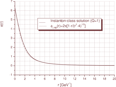
Figure 3: The 1-instanton class solution. The dashed line corresponds to the Yang-Mills instanton.

We first discuss the regular hedgehog solutions. Their three boundary conditions $\phi\left(0\right)=2\pi,$ $\phi^{\prime\prime}\left(0\right)=0$ and $\phi\left(\infty\right)=2\pi\left(1-Q\right)$ imply that for a given $Q$ all of them can be found by varying the initial slope $\beta:=\phi^{\prime}\left(0\right)$. (For the irregular solutions with $\phi\left(0\right)=\pi$ see Ref. [7].) The regular solutions turn out to contain one finite-action solution for each $Q$, denoted as the “$\left|Q\right|$ (anti) instanton class”, and the remaining, continuous (in $\beta$) infinite-action families, the “$2\left|Q\right|$ (anti) meron classes”. The 1-instanton class solution is depicted in Fig. 3. Its relative gauge orientation $U=U_{-}^{-1}U_{+}$ is even quantitatively close to that of the Yang-Mills instanton [14] (orbit) (see dashed curve in Fig. 3). This confirms that the $\left|Q\right|$ instanton classes indeed primarily summarize Yang-Mills instanton contributions. However, they also contain crucial, dilatation-breaking quantum corrections which dynamically stabilize the instanton size at about $\rho\simeq 2\mu^{-1}$, compatible with instanton liquid model [14] and lattice [15] results, and thus overcome the chronic IR instabilities of classical Yang-Mills instanton gases. Since instanton effects play important roles in Yang-Mills theory (e.g. in the $\theta$ vacuum [16] and in spin-0 glueball physics [12, 14, 17]), it is crucial that they are (at least partly) included in the vacuum functional (1). In fact, approximate non-hedgehog solutions corresponding dominantly to ensembles of instantons and anti-instantons should also exist and play prominent roles (since they would be enhanced by a large “entropy”, as in phenomenologically successful “instanton liquid” models [14]).

All remaining regular (i.e. $\phi\left(0\right)=2\pi$) hedgehog solutions, with initial slopes $\beta$ between the discrete instanton-class values $\beta_{I,Q}$, form the $2\left|Q\right|$ (anti-) meron classes. Those approach one of the values $\phi_{M}\left(\infty\right)=\left(2k+1\right)\pi$ at spacial infinity and therefore have infinite action, as the Yang-Mills merons [16]. Moreover, solutions with $\phi\left(\infty\right)=\left(2k+1\right)\pi$, corresponding to an odd number of merons, carry the half-integer topological charge $Q$ of their Yang-Mills meron counterparts. In addition, quantum effects ensure that our meron-class solutions acquire a finite size and therefore remain nonsingular. Since the $2\left|Q\right|$-meron classes appear in continuous families (parametrized by their “size” $\beta^{-1}$), furthermore, their large entropy will help to overcome their infinite-action suppression in functional integrals. As in Yang-Mills theory, merons could then play a physical role, e.g. in the confinement mechanism [16].

We conclude our discussion of selected saddle-point solutions with one of the most intriguing classes, consisting of (solitonic) links and knots. Those emerge from a generalization of Faddeev-Niemi theory [18],

$$\mathcal{L}^{\left(\phi_{k}\right)}\left(\vec{x}\right)=\frac{\mu}{g^{2}\left(\mu\right)}\left[\left(\partial_{i}\hat{n}^{a}\right)^{2}+\frac{1}{\mu^{2}}\left(\varepsilon^{abc}\partial_{i}\hat{n}^{b}\partial_{j}\hat{n}^{c}\right)^{2}+\frac{1}{2\mu^{2}}\left(\varepsilon^{abc}\hat{n}^{b}\partial^{2}\hat{n}^{c}\right)^{2}\right],$$ (35)

which is included in our soft-mode Lagrangian for constant $\phi_{k}=\left(2k+1\right)\pi$. The corresponding solution classes $U_{<}\left(\hat{n}\right)$ describe twists, linked loops and knots made of closed color fluxtubes. Since Eq. (35) follows uniquely from the VWF (1) and the Yang-Mills dynamics, our approach provides a new framework and physical interpretation for such solutions. In fact, they remerge as gauge-invariant IR degrees of freedom representing sets of gauge-field orbits with a collective Hopf charge. While the $\hat{n}$ field of the Faddeev-Niemi model is interpreted as a gauge-dependent local color direction in the vacuum, in particular, our $\hat{n}$ is manifestly gauge-invariant. This may put the tentative interpretation of such knot solutions as glueballs on a firmer basis.

5 Summary and conclusions

We have studied gauge-invariant wave functionals for the Yang-Mills vacuum which incorporate asymptotic freedom and an a priori general dispersion for the infrared gluons in Gaussian core functionals. In this at present probably richest analytically manageable and gauge-invariant trial functional basis, we have then variationally determined several vacuum properties. Dimensional transmutation, dynamical mass generation and gluon condensation emerge transparently and generate mass scales consistent with other approaches. In addition, the improved vacuum description in the infrared predicts a negative kinetic mass of the soft gauge-field modes and thus suggests a negative differential color resistance of the Yang-Mills vacuum.

Another benefit of the gauge-invariant framework is that the dynamics can be reformulated as an effective theory which represents sets of gluon orbits as gauge-invariant matrix fields subject to higher-gradient interactions. In this effective theory we have set up a saddle-point expansion to determine the collective fields with maximal impact on functional integrals. These saddle points play the role of gauge-invariant infrared degrees of freedom. They are stabilized by the dynamical mass generation mechanism and inherit a rich topological structure (three topological charges and action bounds of Bogomol’nyi type) from the Yang-Mills gauge group. Moreover, they provide the principal input for a systematic saddle-point expansion of soft amplitudes (such as glueball correlators).

Several of the more symmetric and important saddle-point solution classes have been found explicitly. Among them are topological solitons related to the classical Yang-Mills (multi-) pseudoparticle solutions which mediate tunneling processes in the vacuum. Those generate a gauge-invariant representation of instanton and meron effects which includes quantum fluctuations. The latter stabilize the pseudoparticle sizes dynamically, in particular, and thereby cure the notorious infrared deseases encountered in dilute instanton ensembles. Similar solutions with other types of topological charges exist as well but seem to have no obvious counterparts in classical Yang-Mills theory. One of the most intriguing solution classes, finally, consists of solitonic links and knots. Those emerge from a generalization of Faddeev-Niemi theory which turns out to be embedded in our soft-mode dynamics. Hence in our framework the knot solutions find a new and in particular gauge-invariant physical interpretation, potentially related to glueballs.

- [1] R.P. Feynman, The qualitative behavior of Yang-Mills theory in 2+1 dimensions, Nucl. Phys. B 188, 479 (1981); in Proceedings of the Intl. Workshop Variational calculations in quantum field theory, Wangerooge, Germany, Eds. L. Polley and D.E.L. Pottinger, World Scientific, Singapore (1988).
- [2] R. Jackiw, Analysis on infinite-dimensional manifolds – Schrödinger representation for quantized fields, in Field theory and particle physics, Eds. O.J.P. Eboli, M. Gomes, A. Santoro, World Scientific, Singapore (1990), p. 731.
- [3] J. Greensite, Calculation of the Yang-Mills vacuum wave functional, Nucl. Phys. B 158, 469 (1979); J. Cornwall, Nonperturbative treatment of the functional Schrödinger equation in QCD, Phys. Rev. D 38, 656 (1988); A.K. Kerman and D. Vautherin, Variational calculations in gauge theories, Ann. Phys. (N.Y.) 192, 408 (1989).
- [4] A.P. Szczepaniak, Confinement and gluon propagator in Coulomb-gauge QCD, Phys. Rev. D 69, 074031 (2004); C. Feuchter and H. Reinhardt, Variational solution of the Yang-Mills Schrödinger equation in Coulomb gauge, Phys. Rev. D 70, 105021 (2004).
- [5] H. Forkel, Gauge-invariant and infrared-improved variational analysis of the Yang-Mills vacuum wave functional, Phys. Rev. D 81, 085030 (2010).
- [6] I.I. Kogan and A. Kovner, Variational approach to the QCD wave functional, Phys. Rev. D 52, 3719 (1995).
- [7] H. Forkel, Infrared degrees of freedom of Yang-Mills theory in the Schrödinger representation, Phys. Rev. D 73, 105002 (2006); Gauge-invariant soft modes in Yang-Mills theory, Int. J. Mod. Phys. E 16, 2789 (2007).
- [8] H. Leutwyler, Constant gauge fields and their quantum fluctuations, Nucl. Phys. B 179, 129 (1981).
- [9] K. Zarembo, Ground state in gluodynamics and quark confinement, Phys. Lett. B 421, 325 (1998).
- [10] D.I. Diakonov, Trying to understand confinement in the Schrödinger picture, lectures given at the 4th St. Petersburg Winter School in Theoretical Physics (1998), arXiv:hep-th/9805137.
- [11] W.E. Brown, Equivalence of the function of the variational approach to that of QCD, Int. J. Mod. Phys. A 13, 5219 (1998).
- [12] H. Forkel, Direct instantons, topological charge screening and QCD glueball sum rules, Phys. Rev. D 71, 054008 (2005); Proceedings of Continuous advances in QCD, Minneapolis, 2006, p. 283 (World Scientific, Singapore, 2007) [arXiv:hep-ph/0608071].
- [13] For an alternative approach see J.M. Cornwall, J. Papavassiliou and D. Binosi, The Pinch Technique and its Applications to Non-Abelian Gauge Theories, Cambridge University Press, Cambridge (UK) (2011).
- [14] T. Schaefer and E.V. Shuryak, Instantons in QCD, Rev. Mod. Phys. 70 (1998) 323; D.I. Diakonov, Instantons at work, Prog. Part. Nucl. Phys. 51 (2003) 173. For an introduction see H. Forkel, A Primer on Instantons in QCD, hep-ph/0009136.
- [15] C. Michael and P.S. Spencer, Cooling and the SU(2) instanton vacuum, Phys. Rev. D 52 (1995) 4691; T. DeGrand, A. Hasenfratz and T.G. Kovacs, Topological structure in the SU(2) vacuum, Nucl. Phys. B 505 (1997) 417; Ph. de Forcrand, M. Garcıa Perez and I.-O. Stamatescu, Topology of the SU(2) vacuum – a lattice study using improved cooling, Nucl. Phys. B 499 (1997) 409.
- [16] C.G. Callan, R.F. Dashen and D. J. Gross, Toward a theory of the strong interactions, Phys. Rev. D 17, 2717 (1978).
- [17] H. Forkel, Holographic glueball structure, Phys. Rev. D 78, 025001 (2008); Glueball correlators as holograms, arXiv:0808.0304 [hep-ph]; PoS (CONFINEMENT8) 184 (2008).
- [18] L.D. Faddeev, Quantization of Solitons, preprint IAS-75-QS70; L.D. Faddeev and A.J. Niemi, Stable knot-like structures in classical field theory, Nature 387 (1997) 58.