Dynamic stabilization of the optical resonances of single nitrogen-vacancy centers in diamond

Abstract

We report electrical tuning by the Stark effect of the excited-state structure of single nitrogen-vacancy (NV) centers located $\lesssim 100~{}{\rm nm}$ from the diamond surface. The zero-phonon line (ZPL) emission frequency is controllably varied over a range of $300~{}{\rm GHz}$. Using high-resolution emission spectroscopy, we observe electrical tuning of the strengths of both cycling and spin-altering transitions. Under resonant excitation, we apply dynamic feedback to stabilize the ZPL frequency. The transition is locked over several minutes and drifts of the peak position on timescales $\gtrsim 100~{}{\rm ms}$ are reduced to a fraction of the single-scan linewidth, with standard deviation as low as 16 MHz (obtained for an NV in bulk, ultra-pure diamond). These techniques should improve the entanglement success probability in quantum communications protocols.

Integrated photonic networks based on cavity-coupled solid-state spin impurities offer a promising platform for scalable quantum computing O’Brien (2007); Stephens et al. (2008); Benjamin et al. (2009); Ladd et al. (2010); Santori et al. (2010). A key ingredient for this technology is the generation and interference of indistinguishable photons emitted by pairs of identical spin qubits Cabrillo et al. (1999); Childress et al. (2005); Moehring et al. (2007). This requires spectrally stable emitters with identical level structure, a formidable challenge in the solid-state environment.

A potential solution is to use external control to counteract sample inhomogeneities. In candidate systems based on single molecules Orrit et al. (1992); Wild et al. (1992); Lettow et al. (2010), quantum dots Empedocles and Bawendi (1997); Patel et al. (2010), and negatively-charged nitrogen-vacancy (NV) centers in diamond Tamarat et al. (2006); Bassett et al. (2011); Bernien et al. (2012), the level structure can be statically tuned via the DC Stark effect. However, the spectral stability of emitters in these systems is often hampered by local fluctuations which cause the emission frequency to change with time, a phenomenon known as spectral diffusion Ambrose and Moerner (1991). Previous attempts to address this problem have focused on improving the host material Jelezko et al. (1997); Santori et al. (2002); Tamarat et al. (2006); Greentree et al. (2006) or using post-selection techniques Ates et al. (2009); Robledo et al. (2010); Togan et al. (2010); Bernien et al. (2012), but a robust, high-yield solution is still lacking.

The diamond NV center is an attractive spin qubit, as it exhibits a unique combination of long-lived spin coherence Balasubramanian et al. (2009) and efficient optical control and readout Buckley et al. (2010); Robledo et al. (2011). However integration into on-chip photonic networks requires NV centers to be located near nanostructured surfaces, where inhomogenous strain and spectral diffusion can be particularly problematic Fu et al. (2010); Faraon et al. (2011). In this Letter, we first demonstrate electrical control over the zero-phonon line (ZPL) transition frequencies, as well as probabilities for both cycling and $\Lambda$-type transitions, of single NV centers located near the diamond surface. We then show that spectral diffusion of the ZPL can be suppressed to 16 MHz standard deviation, on timescales $\gtrsim 100~{}{\rm ms}$, by providing rapid electrical feedback to compensate for local field fluctuations.

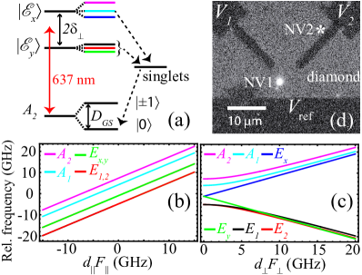
Figure 1: (a) NV level structure at high transverse field ($d_{\perp}F_{\perp}\equiv\delta_{\perp}>15~{}{\rm GHz}$). Dashed lines indicate the spin-selective decay path responsible for optical pumping. (b) Effect of longitudinal and (c) transverse electric fields on the excited state levels. (d) Fluorescence micrograph of the electrode structure. NV1 was illuminated by 532 nm light and appears white, while the position of NV2 is denoted with an asterisk. Metal electrodes appear as shadows.

The negatively-charged nitrogen-vacancy (NV) center has $C_{3v}$ symmetry, and the basic energy structure is depicted in Fig. 1(a). The spin-triplet ground state, ${{}^{3}}A_{2}$, is split such that the $m_{s}=0$ spin projection (labeled $|0\rangle$ throughout) is separated from the degenerate $m_{s}=\pm 1$ levels ($|\pm 1\rangle$) by $D_{GS}=2.88~{}{\rm GHz}$ at $T\lesssim 100~{}{\rm K}$ Acosta et al. (2010a). The optically excited state (ES) is a spin triplet and orbital doublet with ${{}^{3}}E$ symmetry, and its fine structure has been studied theoretically in detail Doherty et al. (2011); Maze et al. (2011). The Hamiltonian describing the ES manifold is:

$$\mathscr{H}_{ES}=\mathscr{H}_{SO}+\mathscr{H}_{SS}+\mathscr{H}_{Stark},$$

$$\mathscr{H}_{Stark}=-\vec{d}\cdot\vec{F},$$ (1)

where $\mathscr{H}_{SO}$, $\mathscr{H}_{SS}$, and $\mathscr{H}_{Stark}$ contain respectively, the spin-orbit, spin-spin, and Stark effect contributions; $\vec{d}$ is the electric dipole moment, and $\vec{F}$ is the electric field. The effect of a strain is treated as an effective electric field Hughes and Runciman (1967); Davies and Hamer (1976).

We first consider the influence of $\mathscr{H}_{Stark}$ on only the orbital portion of the ES wavefunction, consisting of two eigenstates, $\{|\mathscr{E}_{x}\rangle,|\mathscr{E}_{y}\}\rangle$, initially degenerate at zero field. Under electric fields, the orbitals exhibit energy shifts, $\Delta(\vec{F})$, of:

$$\Delta_{\mathscr{E}_{x}}(\vec{F}) =d_{\parallel}F_{\parallel}+d_{\perp}F_{\perp},$$

$$\Delta_{\mathscr{E}_{y}}(\vec{F}) =d_{\parallel}F_{\parallel}-d_{\perp}F_{\perp},$$ (2)

where the directions are with respect to the NV symmetry axis. Longitudinal fields do not lift the orbital degeneracy and result only in equal, linear shifts of all levels. Transverse fields split the orbitals into two branches with an energy difference, $2\delta_{\perp}\equiv(\Delta_{\mathscr{E}_{x}}-\Delta_{\mathscr{E}_{y}})$, that grows linearly with increasing field. The spacings between ground-state sublevels remain relatively unaffected by electric fields van Oort and Glasbeek (1990); Dolde et al. (2011). The ground state may have a longitudinal dipole moment, $d_{GS,\parallel}$ Maze et al. (2011); Doherty et al. (2011), but in experiments we only resolved $\Delta d_{\parallel}\equiv d_{\parallel}-d_{GS,\parallel}$,

Incorporating spin interactions results in a set of six eigenstates, $\{|A_{2}\rangle,|A_{1}\rangle,|E_{x}\rangle,|E_{y}\rangle,|E_{1}\rangle,|E_{2}\rangle\}$, ordered from highest to lowest energy (at low field). Figures 1(b) and (c) show the effect of $\mathscr{H}_{ES}$ on all six ES energies due to, respectively, $F_{\parallel}$ and $F_{\perp}$.

We focused most of our study on NV centers close to the diamond surface, a necessary feature for future integration with nanophotonic devices. Our sample, described in detail elsewhere Stacey et al. (2012); A. Stacey, D. A. Simpson, T. J. Karle, B. C. Gibson, V. Acosta, Z. Huang, K-M. C. Fu, C. Santori, R. G. Beausoleil, L. P. McGuinness, K. Ganesan, S. Tomljenovic-Hanic, A. D. Greentree and Prawer (2012), consists of a high-purity single-crystal, [100]-oriented diamond substrate with a $\sim 100~{}{\rm nm}$ thick chemical-vapor-deposition-grown layer with [NV]$\approx 10^{6}~{}{\rm cm^{-2}}$. The two NV centers studied in this work, labeled NV1 and NV2, are located in this surface layer A. Stacey, D. A. Simpson, T. J. Karle, B. C. Gibson, V. Acosta, Z. Huang, K-M. C. Fu, C. Santori, R. G. Beausoleil, L. P. McGuinness, K. Ganesan, S. Tomljenovic-Hanic, A. D. Greentree and Prawer (2012). Lithographically-defined metal electrodes Bassett et al. (2011) were deposited on the surface [Fig. 1(d)]. The layout of the electrodes (labeled $V_{1},V_{2}$ and $V_{\mathrm{ref}}$) permits tuning of electric fields in any in-plane direction near the center of the structure [Supplementary Information].

A confocal microscope was used to excite and collect emitted light from a diamond sample in thermal contact with the cold finger of a flow-through, liquid-helium cryostat. The cold finger was maintained at a temperature $T\approx 7~{}{\rm K}$, and no magnetic field was applied. Two forms of spectroscopy were employed: high-resolution emission spectroscopy and photoluminescence excitation spectroscopy.

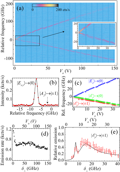
Figure 2: (a) Stark emission spectroscopy. $V_{a}$ was slowly scanned ($1~{}{\rm V/min}$) and emission spectra were obtained in one-minute intervals. A dark exposure frame was taken every 8th frame (cyan vertical stripes). Emission frequencies are relative to $470.45~{}{\rm THz}~{}(637.25~{}{\rm nm})$. Low-field data are inset. (b) Emission spectrum for $V_{a}=1~{}{\rm V}$ with expected peak positions labeled. The $|E_{x,y}\rangle\rightarrow|0\rangle$ emission line is fit with a Gaussian profile. (c) Low-field peak positions from (a) and global fit based on Eq. (Dynamic stabilization of the optical resonances of single nitrogen-vacancy centers in diamond). Lorentzian fit uncertainty is smaller than the plotted symbols. (d) Total ZPL emission versus $\delta_{\perp}$. The emission rate was calculated by subtracting the mean background and summing counts over a range of $\sim 3$ FWHM linewidths centered at each peak. Error bars are based on Poissonian noise. (e) Relative intensity of the $|\mathscr{E}_{y}\rangle\rightarrow|\pm 1\rangle$ emission line along with fit (see text).

For emission spectroscopy, $2~{}{\rm mW}$ of 532-nm laser light was focused by a 0.6-numerical-aperture objective onto NV1, exciting through the phonon sideband (PSB) near saturation. The collected emission was spectrally filtered to direct ZPL light ($636\mbox{-}638~{}{\rm nm}$) to a high-resolution grating spectrometer. The optical polarization was chosen to ensure excitation of both orbital branches Fu et al. (2009). Figure 2(a) shows the emission spectra versus voltage, $V_{a}$, applied simultaneously on $V_{1}$ and $V_{\mathrm{ref}}$, with $V_{2}=0$. By varying $V_{a}$ from $0$ to $150~{}{\rm V}$, we observe linear tuning of emission lines over a range exceeding $300~{}{\rm GHz}$. Such a wide tuning range, enabled by the enhanced fields provided by our devices [Supplementary Information], is essential to compensate for the large intrinsic fields typical in nanophotonic devices Faraon et al. (2011).

Depending on the applied voltage, we resolve between one and three emission lines. At $V_{a}\approx 1~{}{\rm V}$ we observe a single emission line [Fig. 2(b)] with full-width-at-half-maximum (FWHM) linewidth of $1.4(2)~{}{\rm GHz}$, near the spectrometer resolution of $\sim 0.9~{}{\rm GHz}$. We interpret this peak as containing unresolved contributions from the $|E_{x,y}\rangle\rightarrow|0\rangle$ cycling transitions Tamarat et al. (2008); Batalov et al. (2009). Taking into consideration the absence of other peaks, in particular the $|A_{2}\rangle\rightarrow|\pm 1\rangle$ cycling transition Togan et al. (2010), and the observed noise floor, we place a bound on the ground-state spin polarization $\mathscr{P}_{GS}\equiv P_{0}/(P_{0}+P_{\pm 1})\gtrsim 90\%$, where $P_{i}$ is the occupation probability of state $|i\rangle$.

Upon application of transverse fields, the spin character of the levels in the upper $|\mathscr{E}_{x}\rangle$ orbital branch, $\{|A_{2}\rangle,|A_{1}\rangle,|E_{x}\rangle\}$, remain relatively unperturbed. In contrast, the spin character of levels in $|\mathscr{E}_{y}\rangle$, $\{|E_{y}\rangle,|E_{1}\rangle,|E_{2}\rangle\}$, mix at avoided crossings due to spin-spin interaction Santori et al. (2006a); Tamarat et al. (2008); Doherty et al. (2011); Maze et al. (2011), making these levels useful for spin-altering $\Lambda$ schemes.

In the range $5~{}{\rm V}\lesssim V_{a}\lesssim 35~{}{\rm V}$, three emission lines are visible [inset of Fig. 2(a)]. Based on the positive, linear tuning, the upper peak is identified as $|E_{x}\rangle\rightarrow|0\rangle$. Lorentzian fits to these spectra reveal that the two lowest lines are on average separated by $2.7(2)~{}{\rm GHz}$, which is comparable to $D_{GS}$. Considering also the negative, linear tuning, we conclude that these peaks arise from $|\mathscr{E}_{y}\rangle\rightarrow|0\rangle$ and $|\mathscr{E}_{y}\rangle\rightarrow|\pm 1\rangle$ emission (the three levels within $|\mathscr{E}_{y}\rangle$ are nearly degenerate and unresolved here). The presence of these lines was previously predicted based on observations of spin-altering $\Lambda$-type transitions involving the lower orbital branch Santori et al. (2006a, b); Tamarat et al. (2008). Figure 2(c) plots the emission frequencies along with a fit using a model based on Eq. (Dynamic stabilization of the optical resonances of single nitrogen-vacancy centers in diamond), showing excellent agreement. The fitted parameters are $\Delta d_{\parallel}F_{\parallel}/V_{a}=0.42(2)~{}{\rm GHz/V}$ and $d_{\perp}F_{\perp}/V_{a}=1.03(3)~{}{\rm GHz/V}$.

Even with significant emission to $|\pm 1\rangle$, we still do not observe $|A_{2}\rangle\rightarrow|\pm 1\rangle$ emission. Throughout, we find $\mathscr{P}_{GS}\gtrsim 85\%$. A likely explanation is that any population in $|\pm 1\rangle$ is quickly transferred to the metastable singlet levels Acosta et al. (2010b), preventing the detection of $m_{s}=\pm 1$ emission lines. This is consistent with Fig. 2(d), where the total ZPL emission rate integrated over all lines is plotted as a function of one half the orbital splitting, $\delta_{\perp}$. Between $3\lesssim\delta_{\perp}\lesssim 10~{}{\rm GHz}$ ($3\lesssim V_{a}\lesssim 10~{}{\rm V}$), the emission rate falls precipitously before leveling off at less than half the initial rate.

The relative intensity of the emission lines gives further insight into the ES properties. Figure 2(e) plots the intensity of the $|\mathscr{E}_{y}\rangle\rightarrow|\pm 1\rangle$ emission line, normalized by the total emission from $|\mathscr{E}_{y}\rangle$, as a function of $\delta_{\perp}$. Evidently, the applied field is a powerful knob in tuning the relative transition strengths in this $\Lambda$ system. Two peaks for the emission of $|\mathscr{E}_{y}\rangle\rightarrow|\pm 1\rangle$ are present at $\delta_{\perp}\approx 7$ and $15~{}{\rm GHz}$. These features correspond to level anticrossings [see Fig. 1(c)], where maximal mixing of levels in the lower orbital branch occurs. The degree of mixing depends sensitively on both the magnitude of the transverse electric field and its angle, $\theta_{r}$, with respect to the $C_{3v}$ reflection planes Tamarat et al. (2008). We model the relative emission intensity by assuming the NV center is excited from $|0\rangle$ to one of the three levels in the lower branch, $|\mathscr{E}_{y,i}\rangle$. The probability that emission is back to $|\pm 1\rangle$ is then $\sum_{i}P_{0,i}(\theta_{r},\delta_{\perp})(1-P_{0,i}(\theta_{r},\delta_{\perp}))$, where $P_{0,i}(\theta_{r},\delta_{\perp})$ is calculated by taking the overlap of $|\mathscr{E}_{y,i}\rangle$ with $m_{s}=0$ and tracing over orbital degrees of freedom. Here we assume all levels in $|\mathscr{E}_{y}\rangle$ couple equally to the singlets. Using the model based on Eq. (Dynamic stabilization of the optical resonances of single nitrogen-vacancy centers in diamond), we fit this formula to the data and find good agreement for $\theta_{r}=15(5)^{\circ}$.

Finally, we also observe a strong dependence of the relative emission between the upper and lower branches on $\delta_{\perp}$ [Fig. 2(a)]. Given the low temperature $T=7~{}{\rm K}$, this may be due to a single-phonon orbital relaxation process. Phonon decay to the lower branch could contribute to the decreased total emission in Fig. 2(d). A detailed study will be the focus of future work. All of the effects described above were reproduced in subsequent voltage scans [Supplementary Information].

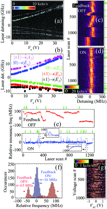
Figure 3: (a) PLE spectra versus applied voltage for NV1. A $532~{}{\rm nm}$ repump pulse ($2.5~{}{\rm\mu W}$, $1~{}{\rm s}$ duration) was applied every $60~{}{\rm s}$. (b) Fitted transition frequencies from (a) and global fit based on Eq. (Dynamic stabilization of the optical resonances of single nitrogen-vacancy centers in diamond), with transitions labeled. (c) PLE spectra for a single NV in the Ural sample ($|0\rangle\rightarrow|E_{x}\rangle$) at $V_{a}=-4~{}{\rm V}$. Green arrows indicate when the repump was applied. (d) PLE spectra for the same NV with voltage feedback applied. (e) Fitted peak positions for scans in (c) [upper panel] and (d) [lower panel]. The recovery under feedback after two separate repump pulses are inset. (f) Histogram of the peak positions in (e). (g) $100~{}{\rm s}$ segment of PLE spectra on NV2 obtained by rapidly scanning a voltage, $V_{AC}$, with feedback applied to $V_{DC}$.

To realize even higher spectral resolution, we performed photoluminescence excitation (PLE) spectroscopy. Attenuated light ($\sim 60~{}{\rm nW}$) from a tunable, external-cavity diode laser ($\sim 637~{}{\rm nm}$) was used for ZPL excitation near saturation, and the collected light was filtered to direct PSB emission ($650\mbox{-}800~{}{\rm nm}$) to a single-photon-counting detector. Microwaves resonant with the ground-state spin transition, $D_{GS}=2.877~{}{\rm GHz}$, were continuously applied to counteract optical pumping Jelezko et al. (2002); Tamarat et al. (2008), and light from a repump laser ($532~{}{\rm nm}$) was occasionally employed to reverse photoionization Drabenstedt et al. (1999); Santori et al. (2006b); Waldherr et al. (2011).

Figure 3(a) plots PLE spectra for NV1 as a function of $V_{a}$, applied simultaneously to $V_{\mathrm{ref}}$ and $V_{1}$, with $V_{2}=0$. Several excitation lines are resolved due to the presence of resonant microwave excitation. We fit the five strongest lines with Lorentzian profiles. The extracted peak positions are plotted in Fig. 3(b) along with a global fit to the model based on Eq. (Dynamic stabilization of the optical resonances of single nitrogen-vacancy centers in diamond), yielding Stark coefficients $\Delta d_{\parallel}F_{\parallel}/V_{a}=0.11(1)~{}{\rm GHz/V}$ and $d_{\perp}F_{\perp}/V_{a}=0.26(2)~{}{\rm GHz/V}$. These coefficients are about four times smaller than those realized under strong $532~{}{\rm nm}$ excitation, consistent with recent observations of enhanced electrical tuning due to photoionization Bassett et al. (2011); Bernien et al. (2012).

We note that the average linewidth for single scans Fu et al. (2009) was $\Gamma_{\mathrm{ss}}=0.14(3)~{}{\rm GHz}$ for NV1 and $\Gamma_{\mathrm{ss}}=0.48(8)~{}{\rm GHz}$ for NV2. In both cases, $\Gamma_{\mathrm{ss}}$ is much broader than the natural linewidth, $\Gamma_{\mathrm{nat}}\approx 13~{}{\rm MHz}$, and is independent of scan rate up to $\sim 20~{}{\rm GHz/s}$. This property requires further investigation, as $\Gamma_{\mathrm{ss}}\approx\Gamma_{\mathrm{nat}}$ has been observed elsewhere Tamarat et al. (2006); Fu et al. (2009); Bernien et al. (2012).

A likely cause for NV spectral diffusion is charge dynamics due to photoionization of nearby defects.To investigate, we use PLE spectroscopy in a different device on the $|0\rangle\rightarrow|E_{x}\rangle$ transition of a single NV center in natural, type IIa (Ural) diamond. This sample was chosen due to the much narrower linewidth, $\Gamma_{\mathrm{ss}}=60(7)~{}{\rm MHz}$, even after $\sim 15~{}{\rm MHz}$ of power broadening. Figure 3(c) shows typical PLE spectra for $200~{}{\rm ms}$ scans with repump pulse ($\sim 10~{}{\rm\mu W}$, $20~{}{\rm ms}$ duration) applied only after the NV center had photoionized. The transition frequency drifts over a range significantly larger than $\Gamma_{\mathrm{ss}}$ during the $280~{}{\rm s}$ data set.

Our solution to the spectral-drift problem is to actively adjust $V_{a}$ to compensate for the changing local field. We start with $V_{a}=-4~{}{\rm V}$, and, during the back-scan of subsequent scans (final $10\%$ of each cycle), we employ software-controlled feedback with the following algorithm. We first determine the position and intensity of the peak fluorescence. If the intensity falls below a threshold, we apply a repump pulse and do not change $V_{a}$. Otherwise, we change $V_{a}$ based on optimized proportionality and integration inputs [Supplementary Information].

Figure 3(d) shows PLE spectra under similar conditions as Fig. 3(c) but now with feedback applied. While $\Gamma_{\mathrm{ss}}$ remains unchanged, the center-frequency drift is substantially reduced. We fit the spectra in Figs. 3(c) and (d) with Lorentzian profiles and plot the extracted peak positions in Fig. 3(e). In the case of no feedback, two mechanisms of spectral drift are identified: large instantaneous jumps following application of the repump and slower drift in between repump pulses. Under feedback, spectral jumps still accompany repump pulses, but these are quickly compensated for. Two spectral jumps with the slowest recovery, $5\mbox{-}10$ scans, are shown as insets. A figure of merit for the total drift is obtained by plotting the histogram of fitted peak positions from all PLE scans and determining the resulting standard deviation, $\sigma$ [Fig. 3(f)]. Without feedback, we find a non-uniform profile with $\sigma\approx 65~{}{\rm MHz}$. Under feedback, $\sigma=16~{}{\rm MHz}$, which is smaller than $\Gamma_{\mathrm{ss}}$ and comparable to $\Gamma_{\mathrm{nat}}$.

This feedback technique can be applied at significantly higher bandwidth (here, up to $20~{}{\rm Hz}$ scan repetition rate) without compromising stability. Throughout, we find that feedback reduces $\sigma$ to a fraction of $\Gamma_{\mathrm{ss}}$. Similar results were obtained for NV1 and NV2 [Supplemental Information] as well as for stabilizing the $|\pm 1\rangle\rightarrow{A_{2}}$ transition.

It is often advantageous to perform experiments with the excitation laser frequency fixed to an external reference. In this case, voltage feedback can still be employed by sweeping the ZPL transition frequency using an AC voltage, $V_{AC}$, and providing stabilizing feedback to the DC component, $V_{DC}$. With this technique, feedback can be applied continuously without substantially degrading photon indistinguishability, provided that the modulation depth and laser linewidth are sufficiently small.

Figure 3(g) shows results of locking the NV2 $|0\rangle\rightarrow|E_{x}\rangle$ transition frequency using only applied voltages. We perform PLE spectroscopy as before except, instead of scanning the laser frequency, we ramp the voltage, $V_{AC}$ (applied to $V_{2}$ and $V_{\mathrm{ref}}$), with amplitude $3~{}{\rm V_{pp}}$ and period $0.1~{}{\rm s}$. Meanwhile, $V_{DC}$ is fed back to $V_{1}$, initially starting at $-8~{}{\rm V}$, but varying by $\sim\pm 4~{}{\rm V}$ throughout the $600~{}{\rm s}$ measurement. After background subtraction, we collect on average $144~{}{\rm cts/s}$. This compares favorably to the $34~{}{\rm cts/s}$ collected without feedback (with repump applied every scan). The overall count rate can be further increased with improved collection efficiency Hadden et al. (2010); Hausmann et al. (2012) and resonant Purcell enhancement Faraon et al. (2011, 2012).

In summary, we have used the Stark effect to electrically tune and stabilize the structure of the NV center’s excited state. Applied simultaneously to a pair of NV centers, these techniques pave the way for increased two-photon interference visibilities Patel et al. (2010); Lettow et al. (2010); Bernien et al. (2012) and heralded entanglement success probabilities Moehring et al. (2007).

We acknowledge support by the Defense Advanced Research Projects Agency (award no. HR0011-09-1-0006), the Regents of the University of California, and the Australian Research Council (ARC) (Project Nos. LP100100524, DP1096288, and DP0880466). We thank T. Karle, B. Gibson, T. Ishikawa, B. Buckley, and A. Falk for valuable discussions.

Supplementary Information: Dynamic stabilization of the optical resonances of single nitrogen-vacancy centers in diamond

I Electrostatic modeling

We modeled the electric field produced by the electrode structure in Fig. 1(c) of the main text using the COMSOL MULTIPHYSICS®  electrostatics package. The bottom layer of each electrode is composed of 10 nm of Ti, so for simplicity we model the electrodes as being 100-nm thick, composed entirely of Ti. We use a relative permittivity for the diamond substrate $\epsilon_{r}=5.1$. The positions of NV1 and NV2 were determined by fluorescence micrographs, as in Fig. 1(d) of the main text.

Based on our simulations, application of $10~{}{\rm V}$ to one electrode (with the other two electrodes grounded) corresponds to an electric field amplitude at the location of NV1 of $0.9,0.6,$ and $1.1~{}{\rm MV/m}$, for $V_{1},V_{2},$ and $V_{\mathrm{ref}}$, respectively. In Fig. S1 we plot the in-plane electric field components on the diamond surface for $\{V_{1},V_{2},V_{\mathrm{ref}}\}=\{10,0,10\}~{}{\rm V}$.

As a note of caution: this model assumes a perfect dielectric response. In reality the local field is subject to significant deviations due to charge variations introduced by the electrodes or from photo-ionization Bassett et al. (2011). These deviations do not substantially affect the performance of dynamic ZPL stabilization, since the proportional gain can be adjusted to compensate (see below), but they do play an important role in static tuning. One example is the photo-induced effect that is responsible for the $\sim 4$ times greater Stark tuning coefficients for strong ($2~{}{\rm mW}$) cw green excitation, compared with weak ($\sim 60~{}{\rm nW}$) red excitation, and is discussed in detail in Ref. Bassett et al. (2011).

We also observe hysteretic charging effects which alter the static tuning even with very weak $(\lesssim 60~{}{\rm nW}$) red excitation and without applying any green repump. This hysteresis results in a variation of observed tuning coefficients which depends on scan direction, rate, and history. The variation exists even between successive voltage scans as short as 10 s. Overall, the observed tuning coefficients vary by up to a factor of 5, making a measurement of the intrinsic dipole moment of the NV center a difficult task. Using the Stark tuning coefficients for NV1, determined from the $\sim 2~{}{\rm hr}$ forward voltage scan in Fig. 3(a) of the main text, the dipole moment is $\{\Delta d_{\parallel},d_{\perp}\}\approx\{4,5\}~{}{\rm GHz/MV/m}$, which is probably correct to within a factor of 2-3. For this calculation the magnitude of the applied electric field and its angle with respect to the NV axis were estimated based on the electrostatic modeling in Fig. S1 and the dependence of NV1 fluorescence intensity on excitation light polarization.

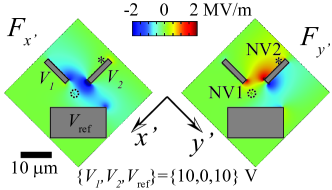
Figure S1: In-plane electric-field components on the diamond surface, $F_{x^{\prime},y^{\prime}}$, for $V_{a}=10~{}{\rm V}$ applied simultaneously to $V_{1}$ and $V_{\mathrm{ref}}$, with $V_{2}=0$. The locations of NV1 (dashed circle) and NV2 (asterisk) are shown, as in Fig. 1 of the main text. The out-of-plane component $F_{z^{\prime}}\approx 0$.

II Reproducibility of emission spectroscopy

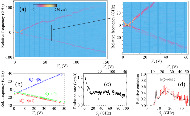
Figure S2: (a) Stark emission spectra as a function of applied voltage on $V_{1}$, with $V_{2}=V_{\mathrm{ref}}=0$. Low-field data are displayed on the right. (b) Low-field peak positions determined from Lorentzian fits (symbols) and global fit. Lorentzian fit uncertainty is smaller than the plotted symbols. (c) Total ZPL emission versus $\delta_{\perp}$. (d) Relative intensity of the $|\mathscr{E}_{y}\rangle\rightarrow|\pm 1\rangle$ emission line along with fit. The methods for fitting and processing spectra are described in the main text.

The reproducibility of Stark emission spectroscopy results was tested by varying the voltage on various combinations of electrodes. Figure S2(a) shows emission spectra while varying the voltage applied to $V_{1}$, with $V_{2}=V_{\mathrm{ref}}=0$. Despite the continuous voltage tuning, small kinks in the emission lines are observed, particularly following dark frames. During the dark frames of this particular data set, we performed a peak-finding procedure that locates the optical focal position which produces maximum NV emission. The resulting shifts in optical focus may produce small changes in the local field due to photo-induced charge redistribution Bassett et al. (2011); Bernien et al. (2012). In Fig. 2 of the main text we used a different procedure to maintain optical focus based on continuous feedback using a weak white-light reflection image. This may explain the absence of sharp kinks in the Stark emission spectra in Fig. 2(a).

The inset of Fig. S2(a) shows the low-field spectra, with three emission lines clearly visible. As in Fig. 2 of the main text, we do not observe $|A_{2}\rangle\rightarrow|\pm 1\rangle$ emission, indicating ground-state spin polarization, $\mathscr{P}_{GS}\gtrsim 85\%$. Following the procedure outlined in the main text, we fit these spectra [Fig. S2(b)] and found Stark coefficients of $\Delta d_{\parallel}F_{\parallel}/V_{a}=0.26(2)~{}{\rm GHz/V}$ and $d_{\perp}F_{\perp}/V_{a}=0.81(4)~{}{\rm GHz/V}$. In Fig. S2(c), the total emission intensity as a function of $\delta_{\perp}$ is plotted. These data are qualitatively similar to that found in Fig. 2(d) of the main text. In Fig. S2(d), the emission intensity of the $|\mathscr{E}_{y}\rangle\rightarrow|\pm 1\rangle$ line, relative to the total emission from $|\mathscr{E}_{y}\rangle$, is plotted versus $\delta_{\perp}$. Based on the fit, we find $\theta_{r}=12(5)^{\circ}$.

III feedback optimization

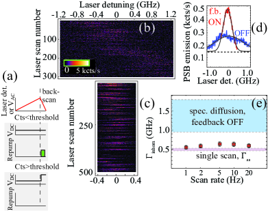
Figure S3: (a) Timing diagram of the feedback protocol described in the text. (b) PLE spectra for NV2 ($|0\rangle\rightarrow|E_{x}\rangle$) with $V_{a}=-4~{}{\rm V}$. The scan rate was $1~{}{\rm Hz}$, and a repump pulse ($10~{}{\rm\mu W}$, $0.1~{}{\rm s}$) was applied during every back-scan. (c) PLE spectra for NV2 with feedback applied. The enhanced spectral stability allowed us to reduce the laser-frequency scan range by a factor of four. (d) Sum over the scans in (b) and (c) with, respectively, feedback off (blue) and on (red) along with Gaussian fits (solid black lines) using the mean background of $150~{}{\rm cts/s}$ (black dashed line). (e) Comparison of $\Gamma_{\mathrm{inhom}}$ as a function of scan repetition rate. The spectral-diffusion-broadened linewidth (blue shaded region) is the range observed over data sets taken without feedback with 1, 2, 5, 10 and $20~{}{\rm Hz}$ scan rates.

The basic feedback protocol is described in the text, and here we outline experimental details. All PLE scans used a ramp waveform with $90\%$ duty cycle. In other words, we scan either the laser frequency or $V_{AC}$ in one direction for $90\%$ of the total scan cycle and the final $10\%$ is devoted to scanning back in the other direction (the “back-scan”). We divide our collected PSB counts into bins of variable size, typically forming $10\mbox{-}50$ bins in total. During the backscan of each cycle (denoted with index $i$), we search for the bin location, $b_{i}$, with the maximum counts, $C_{i}$. We set a threshold, $T$, typically corresponding to a count rate of $1~{}{\rm kcts/s}$, much larger than the background signal off resonance. If $C_{i}<T$, we apply a green repump pulse for the remainder of the backscan and do not change $V_{DC}$.

If $C_{i}\geq T$, we do not apply a repump pulse. Instead, we change $V_{DC}$ by an amount $\delta V_{i}$ using the following formula:

$$\delta V_{i}=G\times(B-\frac{1}{N}\sum_{j=0}^{N-1}b_{i-j}).$$ (S1)

Here $G$ is a gain factor, $N$ is an integration factor corresponding to the number of cycles used to determine $\delta V_{i}$, and $B$ is the desired peak position. In our experiments, we typically set $B$ to be the bin at the center of each scan. For all of the laser-frequency scans in the main text [Fig. 3(d)-(f)], we used $N=1$ (no integration). For the $0.1$-s voltage scans we found that feedback was most efficient using $N=2\mbox{-}4$. The $100$-second portion shown in Fig. 3(g) used $N=2$. We separately optimize $G$ based on the NV center’s Stark tuning coefficients as well as the method and rate of scanning. Figure S3(a) depicts a timing diagram of the feedback routine.

We performed the feedback routine discussed above on the $|0\rangle\rightarrow|E_{x}\rangle$ transition of NV2 in the NV-doped surface layer sample. Figure S3(b) shows typical PLE spectra when scanning the excitation laser frequency through resonance and applying a repump after each scan. As mentioned in the main text, the average linewidth for single scans, computed using the technique in Ref. Fu et al. (2009), was $\Gamma_{\mathrm{ss}}=0.48(8)~{}{\rm GHz}$ for NV2. Nonetheless, the ZPL center frequency in Fig. S3(c) drifts over a range significantly larger than $\Gamma_{\mathrm{ss}}$ during the $300~{}{\rm s}$ data set.

Figure S3(c) shows PLE spectra under similar conditions as Fig. S3(c) but now with feedback applied. While $\Gamma_{\mathrm{ss}}$ remains unchanged, the center-frequency drift is substantially reduced. A figure of merit for the spectral drift of the transition is obtained by summing over many PLE scans and determining the resulting inhomogenous linewidth, $\Gamma_{\mathrm{inhom}}$. This figure-of-merit is somewhat different from the histogram technique described in the main text and was employed due to the large single-scan linewidth for this NV center. Figure S3(d) compares the sum of spectra with feedback off [Fig. S3(b)] and on [S3(c)] along with Gaussian fits. Without feedback, we find $\Gamma_{\mathrm{inhom}}=1.8(2)~{}{\rm GHz}\approx 3.8\Gamma_{\mathrm{ss}}$, and with feedback this decreases to $0.54(4)~{}{\rm GHz}\approx 1.1\Gamma_{\mathrm{ss}}$.

This feedback technique can be applied at significantly higher bandwidth without compromising stability. Figure S3(e) plots $\Gamma_{\mathrm{inhom}}$ as a function of scan repetition rate up to $20~{}{\rm Hz}$. Throughout this range, we find $\Gamma_{\mathrm{inhom}}\lesssim 1.3\Gamma_{\mathrm{ss}}$. Future improvements could involve ultra-fast correlation measurements to determine the nature of the broad single-scan linewidth Sallen et al. (2010).

References

- O’Brien (2007) J. L. O’Brien, Science (New York, N.Y.) 318, 1567 (2007).
- Stephens et al. (2008) A. M. Stephens, Z. W. E. Evans, S. J. Devitt, A. D. Greentree, A. G. Fowler, W. J. Munro, J. L. O’Brien, K. Nemoto, and L. C. L. Hollenberg, Physical Review A 78, 032318 (2008).
- Benjamin et al. (2009) S. Benjamin, B. Lovett, and J. Smith, Laser & Photonics Review 3, 556 (2009).
- Ladd et al. (2010) T. D. Ladd, F. Jelezko, R. Laflamme, Y. Nakamura, C. Monroe, and J. L. O’Brien, Nature 464, 45 (2010).
- Santori et al. (2010) C. Santori, P. E. Barclay, K.-M. C. Fu, R. G. Beausoleil, S. Spillane, and M. Fisch, Nanotechnology 21, 274008 (2010).
- Cabrillo et al. (1999) C. Cabrillo, J. I. Cirac, P. García-Fernández, and P. Zoller, Physical Review A 59, 1025 (1999).
- Childress et al. (2005) L. I. Childress, J. M. Taylor, A. Sø rensen, and M. D. Lukin, Physical Review A 72, 052330 (2005).
- Moehring et al. (2007) D. L. Moehring, P. Maunz, S. Olmschenk, K. C. Younge, D. N. Matsukevich, L.-M. Duan, and C. Monroe, Nature 449, 68 (2007).
- Orrit et al. (1992) M. Orrit, J. Bernard, A. Zumbusch, and R. Personov, Chemical Physics Letters 196, 595 (1992).
- Wild et al. (1992) U. P. Wild, F. Güttler, M. Pirotta, and A. Renn, Chemical Physics Letters 193, 451 (1992).
- Lettow et al. (2010) R. Lettow, Y. L. A. Rezus, A. Renn, G. Zumofen, E. Ikonen, S. Götzinger, and V. Sandoghdar, Physical Review Letters 104, 123605 (2010).
- Empedocles and Bawendi (1997) S. A. Empedocles and M. G. Bawendi, Science 278, 2114 (1997).
- Patel et al. (2010) R. B. Patel, A. J. Bennett, I. Farrer, C. A. Nicoll, D. A. Ritchie, and A. J. Shields, Nature Photonics 4, 632 (2010).
- Tamarat et al. (2006) P. Tamarat, T. Gaebel, J. R. Rabeau, M. Khan, A. D. Greentree, H. Wilson, L. C. L. Hollenberg, S. Prawer, P. Hemmer, F. Jelezko, and J. Wrachtrup, Physical Review Letters 97, 083002 (2006).
- Bassett et al. (2011) L. Bassett, F. Heremans, C. Yale, B. Buckley, and D. Awschalom, Physical Review Letters 107 (2011), 10.1103/PhysRevLett.107.266403.
- Bernien et al. (2012) H. Bernien, L. Childress, L. Robledo, M. Markham, D. Twitchen, and R. Hanson, Physical Review Letters 108 (2012), 10.1103/PhysRevLett.108.043604.
- Ambrose and Moerner (1991) W. P. Ambrose and W. E. Moerner, Nature 349, 225 (1991).
- Jelezko et al. (1997) F. Jelezko, B. Lounis, and M. Orrit, The Journal of Chemical Physics 107, 1692 (1997).
- Santori et al. (2002) C. Santori, D. Fattal, J. Vučković, G. S. Solomon, and Y. Yamamoto, Nature 419, 594 (2002).
- Greentree et al. (2006) A. D. Greentree, P. Olivero, M. Draganski, E. Trajkov, J. R. Rabeau, P. Reichart, B. C. Gibson, S. Rubanov, S. T. Huntington, D. N. Jamieson, and S. Prawer, Journal of Physics: Condensed Matter 18, S825 (2006).
- Ates et al. (2009) S. Ates, S. M. Ulrich, S. Reitzenstein, A. Löffler, A. Forchel, and P. Michler, Physical Review Letters 103, 167402 (2009).
- Robledo et al. (2010) L. Robledo, H. Bernien, I. van Weperen, and R. Hanson, Physical Review Letters 105, 177403 (2010).
- Togan et al. (2010) E. Togan, Y. Chu, A. S. Trifonov, L. Jiang, J. Maze, L. Childress, M. V. G. Dutt, A. S. Sorensen, P. R. Hemmer, A. S. Zibrov, and M. D. Lukin, Nature 466, 730 (2010).
- Balasubramanian et al. (2009) G. Balasubramanian, P. Neumann, D. Twitchen, M. Markham, R. Kolesov, N. Mizuochi, J. Isoya, J. Achard, J. Beck, J. Tissler, V. Jacques, P. R. Hemmer, F. Jelezko, and J. Wrachtrup, Nat Mater 8, 383 (2009).
- Buckley et al. (2010) B. B. Buckley, G. D. Fuchs, L. C. Bassett, and D. D. Awschalom, Science (New York, N.Y.) 330, 1212 (2010).
- Robledo et al. (2011) L. Robledo, L. Childress, H. Bernien, B. Hensen, P. F. A. Alkemade, and R. Hanson, Nature 477, 574 (2011).
- Fu et al. (2010) K. M. C. Fu, C. Santori, P. E. Barclay, and R. G. Beausoleil, Applied Physics Letters 96, 121903 (2010).
- Faraon et al. (2011) A. Faraon, P. E. Barclay, C. Santori, K.-M. C. Fu, and R. G. Beausoleil, Nature Photonics 5, 301 (2011).
- Acosta et al. (2010a) V. M. Acosta, E. Bauch, M. P. Ledbetter, A. Waxman, L. S. Bouchard, and D. Budker, Physical Review Letters 104, 70801 (2010a).
- Doherty et al. (2011) M. W. Doherty, N. B. Manson, P. Delaney, and L. C. L. Hollenberg, New Journal of Physics 13, 25019 (2011).
- Maze et al. (2011) J. Maze, A. Gali, E. Togan, Y. Chu, A. S. Trifonov, E. Kaxiras, and M. D. Lukin, New Journal of Physics 13, 25025 (2011).
- Hughes and Runciman (1967) A. E. Hughes and W. A. Runciman, Proceedings of the Physical Society 90, 827 (1967).
- Davies and Hamer (1976) G. Davies and M. F. Hamer, Proceedings of the Royal Society A: Mathematical, Physical and Engineering Sciences 348, 285 (1976).
- van Oort and Glasbeek (1990) E. van Oort and M. Glasbeek, Chemical Physics Letters 168, 529 (1990).
- Dolde et al. (2011) F. Dolde, H. Fedder, M. Doherty, T. Nöbauer, F. Rempp, G. Balasubramanian, T. Wolf, F. Reinhard, L. Hollenberg, F. Jelezko, and Others, Nature Physics 7, 459 (2011).
- Stacey et al. (2012) A. Stacey, T. J. Karle, L. P. McGuinness, B. C. Gibson, K. Ganesan, S. Tomljenovic-Hanic, A. D. Greentree, A. Hoffman, R. G. Beausoleil, and S. Prawer, Applied Physics Letters 100, 071902 (2012).
- A. Stacey, D. A. Simpson, T. J. Karle, B. C. Gibson, V. Acosta, Z. Huang, K-M. C. Fu, C. Santori, R. G. Beausoleil, L. P. McGuinness, K. Ganesan, S. Tomljenovic-Hanic, A. D. Greentree and Prawer (2012) A. Stacey, D. A. Simpson, T. J. Karle, B. C. Gibson, V. Acosta, Z. Huang, K-M. C. Fu, C. Santori, R. G. Beausoleil, L. P. McGuinness, K. Ganesan, S. Tomljenovic-Hanic, A. D. Greentree and S. Prawer, in preparation (2012).
- Fu et al. (2009) K.-M. C. Fu, C. Santori, P. E. Barclay, L. J. Rogers, N. B. Manson, and R. G. Beausoleil, Physical Review Letters 103, 256404 (2009).
- Tamarat et al. (2008) P. Tamarat, N. B. Manson, J. P. Harrison, R. L. McMurtrie, A. Nizovtsev, C. Santori, R. G. Beausoleil, P. Neumann, T. Gaebel, F. Jelezko, P. Hemmer, and J. Wrachtrup, New Journal of Physics 10, 045004 (2008).
- Batalov et al. (2009) A. Batalov, V. Jacques, F. Kaiser, P. Siyushev, P. Neumann, L. J. Rogers, R. L. McMurtrie, N. B. Manson, F. Jelezko, and J. Wrachtrup, Physical Review Letters 102, 195506 (2009).
- Santori et al. (2006a) C. Santori, D. Fattal, S. M. Spillane, M. Fiorentino, R. G. Beausoleil, A. D. Greentree, P. Olivero, M. Draganski, J. R. Rabeau, P. Reichart, B. C. Gibson, S. Rubanov, D. N. Jamieson, and S. Prawer, Optics Express 14, 7986 (2006a).
- Santori et al. (2006b) C. Santori, P. Tamarat, P. Neumann, J. Wrachtrup, D. Fattal, R. G. Beausoleil, J. Rabeau, P. Olivero, A. D. Greentree, S. Prawer, F. Jelezko, and P. Hemmer, Physical Review Letters 97, 247401 (2006b).
- Acosta et al. (2010b) V. M. Acosta, A. Jarmola, E. Bauch, and D. Budker, Physical Review B 82, 201202 (2010b).
- Jelezko et al. (2002) F. Jelezko, I. Popa, A. Gruber, C. Tietz, J. Wrachtrup, A. Nizovtsev, and S. Kilin, Applied Physics Letters 81, 2160 (2002).
- Drabenstedt et al. (1999) A. Drabenstedt, L. Fleury, C. Tietz, F. Jelezko, S. Kilin, A. Nizovtzev, and J. Wrachtrup, Physical Review B 60, 11503 (1999).
- Waldherr et al. (2011) G. Waldherr, J. Beck, M. Steiner, P. Neumann, A. Gali, T. Frauenheim, F. Jelezko, and J. Wrachtrup, Physical Review Letters 106, 157601 (2011).
- Hadden et al. (2010) J. P. Hadden, J. P. Harrison, A. C. Stanley-Clarke, L. Marseglia, Y. L. D. Ho, B. R. Patton, J. L. O’Brien, and J. G. Rarity, Applied Physics Letters 97, 241901 (2010).
- Hausmann et al. (2012) B. J. M. Hausmann, B. Shields, Q. Quan, P. Maletinsky, M. McCutcheon, J. T. Choy, T. M. Babinec, A. Kubanek, A. Yacoby, M. D. Lukin, and M. Loncar, Nano letters (2012), 10.1021/nl204449n.
- Faraon et al. (2012) A. Faraon, C. Santori, Z. Huang, V. M. Acosta, and R. G. Beausoleil, (2012), arXiv:1202.0806 .

References

- Bassett et al. (2011) L. Bassett, F. Heremans, C. Yale, B. Buckley, and D. Awschalom, Physical Review Letters 107 (2011), 10.1103/PhysRevLett.107.266403.
- Bernien et al. (2012) H. Bernien, L. Childress, L. Robledo, M. Markham, D. Twitchen, and R. Hanson, Physical Review Letters 108 (2012), 10.1103/PhysRevLett.108.043604.
- Fu et al. (2009) K.-M. C. Fu, C. Santori, P. E. Barclay, L. J. Rogers, N. B. Manson, and R. G. Beausoleil, Physical Review Letters 103, 256404 (2009).
- Sallen et al. (2010) G. Sallen, A. Tribu, T. Aichele, R. André, L. Besombes, C. Bougerol, M. Richard, S. Tatarenko, K. Kheng, and J.-P. Poizat, Nature Photonics 4, 696 (2010).