Fast computation of high frequency Dirichlet eigenmodes via the spectral flow of the interior Neumann-to-Dirichlet map

Abstract.

We present a new algorithm for numerical computation of large eigenvalues and associated eigenfunctions of the Dirichlet Laplacian in a smooth, star-shaped domain in $\mathbb{R}^{d}$, $d\geq 2$. Conventional boundary-based methods require a root-search in eigenfrequency $k$, hence take $O(N^{3})$ effort per eigenpair found, using dense linear algebra, where $N=O(k^{d-1})$ is the number of unknowns required to discretize the boundary. Our method is $O(N)$ faster, achieved by linearizing with respect to $k$ the spectrum of a weighted interior Neumann-to-Dirichlet (NtD) operator for the Helmholtz equation. Approximations $\hat{k}_{j}$ to the square-roots $k_{j}$ of all $O(N)$ eigenvalues lying in $[k-{\epsilon},k]$, where ${\epsilon}=O(1)$, are found with $O(N^{3})$ effort. We prove an error estimate

$$|\hat{k}_{j}-k_{j}|\leq C\Big{(}\frac{{\epsilon}^{2}}{k}+{\epsilon}^{3}\Big{)},$$

with $C$ independent of $k$. We present a higher-order variant with eigenvalue error scaling empirically as $O({\epsilon}^{5})$ and eigenfunction error as $O({\epsilon}^{3})$, the former improving upon the ‘scaling method’ of Vergini–Saraceno. For planar domains ($d=2$), with an assumption of absence of spectral concentration, we also prove rigorous error bounds that are close to those numerically observed. For $d=2$ we compute robustly the spectrum of the NtD operator via potential theory, Nyström discretization, and the Cayley transform. At high frequencies (400 wavelengths across), with eigenfrequency relative error $10^{-10}$, we show that the method is $10^{3}$ times faster than standard ones based upon a root-search.

1. Introduction

Let $\Omega$ be a smooth, bounded domain in ${\mathbb{R}}^{d}$, strictly star-shaped with respect to the origin, that is $x\cdot n>0$ for each $x\in{\partial\Omega}$ where $n$ is the outward-pointing unit normal vector. We are interested in computing numerically the eigenvalues $k_{j}^{2}$, and eigenfunctions or eigenmodes $\phi_{j}$ (normalized by $\|\phi_{j}\|_{L^{2}(\Omega)}=1$), of the Dirichlet Laplacian $\Delta=\sum_{i=1}^{d}\partial^{2}/\partial_{x_{i}}^{2}$ on $\Omega$. That is,

$$(\Delta+k_{j}^{2})\phi_{j} = 0\qquad\mbox{ in }\Omega~{},$$ (1)

$$\phi_{j} = 0\qquad\mbox{ on }{\partial\Omega}~{}.$$ (2)

We will refer to $k_{j}$, the square-roots of eigenvalues, as (Dirichlet) eigenfrequencies, and order them $0<k_{1}<k_{2}\leq k_{3}\leq\dots$ counting multiplicities. This classical problem has many applications in engineering and physics [20, 4], principally in the modeling of acoustic, electromagnetic and optical cavities, vibrating membranes, trapped quantum particles and nano-scale devices [44], and in data analysis [51]. Note that some applications involve homogeneous boundary conditions other than (2), or the Maxwell or elasticity equations, yet the above serves as a paradigm for this larger class of problems. In $d=2$ it is known as the ‘drum’ problem, and is reviewed in [39, 56]. A numerical approach is needed for all but the small subset of domains $\Omega$ where separation of variables is possible (explicitly, those which are a product of intervals in a coordinate system in which $\Delta$ is separable [20]).

Many applications demand high eigenfrequency $k_{j}$ (i.e. high mode number $j$), which creates a challenging numerical problem. For instance, the design of high-power micro-laser resonators [58] requires $j>10^{3}$ (i.e. tens of wavelengths across the domain). Knowledge of eigenfunctions informs high-frequency wave scattering from resonant structures such as jet engine inlets [38]. Interest has also surged recently in quantum chaos [62, 45] and spectral geometry [28], where numerical studies have played a key role, such as in the discovery of ‘scars’ of periodic ray orbits in chaotic eigenfunctions [30], and the study of eigenfunction equidistribution rates [7, 9]. This can involve computing thousands of modes at up to $j\sim 10^{6}$, i.e. hundreds of wavelengths across the domain [60, 9]. The above motivates the creation of efficient high frequency numerical methods with controlled errors.

Existing numerical methods for (1)-(2) generally fall into two classes:

1. Direct discretization of $\Omega$ (via finite differences or finite elements [4]), which has the advantage that eigenvalues $k_{j}^{2}$ are approximated by the spectrum of a linear (sparse, often generalized) matrix eigenvalue problem. However, since several degrees of freedom per wavelength in each dimension are needed, the number of unknowns $N$ grows at least like $k^{d}$. In fact, to achieve bounded accuracy as $k\to\infty$ an increasing number of unknowns per wavelength are required; this is the so-called ‘pollution effect’ [5]. Iterative methods are needed for such huge eigenvalue problems. We believe the furthest this has been pushed in $d=2$ is $j\sim 3\times 10^{3}$ (around 30 wavelengths across the domain), by Heuveline and others [32, 22, 21]. However, here specialized multigrid and removal of spurious eigenvalues are needed, and relative errors in $k_{j}$ are as high as $10^{-3}$.

2. Boundary-based methods, which make use of a basis of analytic solutions to the Helmholtz equation (1), hence only require discretization of ${\partial\Omega}$ via a much smaller $N=O(k^{d-1})$ unknowns. The main disadvantage is that, since the $k$-dependence of the basis is nonlinear, eigenfrequencies $k_{j}$ are now given by a (dense) nonlinear eigenvalue problem. This generally requires repeated iterative minimization of some error measure along the $k$ axis, which is cumbersome and prone to the omission of eigenfrequencies [6, 57]. The error measure is often a minimum singular value (e.g. see App. B), hence $O(N^{3})$ effort is required per eigenfrequency found.

   This class includes the method of particular solutions (MPS) [15] (also known as collocation, Trefftz, non-polynomial FEM, or ultra-weak variational formulation [16, 42]) which uses plane-wave [30], regular Bessel [17, 52], or corner-adapted Fourier-Bessel solutions [23, 15, 14]; the method of fundamental solutions [33] which uses point sources placed outside of $\Omega$; and boundary integral equation (BIE, also known as boundary element) methods which make use of potential theory on ${\partial\Omega}$ [19]. Such methods often have spectral (i.e. super-algebraic) error convergence, although most BIE implementations remain low-order [35, 6, 24, 59]. They can easily reach $j=10^{4}$, with relative errors as small as $10^{-14}$ [12], and variants have reached $j>10^{6}$ [60, 57].

Can one combine the advantages of classes A and B, i.e. is there a boundary-based method that does not require a root search for each eigenfrequency? This was answered, in the case of star-shaped domains, by Vergini–Saraceno [61] who proposed a ‘scaling method’—reviewed in section 7— which may be viewed as an acceleration technique for the MPS. Here a single dense matrix eigenvalue problem, i.e. effort $O(N^{3})$, approximates all eigenfrequencies (and their eigenfunctions) lying in an interval of the $k$ axis of length ${\epsilon}=O(1)$. Since by Weyl’s law [26, Ch. 11] one expects $O(k^{d-1})$ such eigenfrequencies, this is also the speed-up factor of the method, assuming errors are acceptable. The absolute eigenfrequency error is empirically $O({\epsilon}^{3})$ [8, 9], although this has scarcely been studied. The scaling method has allowed large-scale studies of quantum chaos to be performed in $d=2$ [60, 9, 11] and $d=3$ [48] at speeds around $10^{3}$ times faster than any other known method.

This key idea of linearizing the nonlinear eigenvalue problem in class B has been noticed by couple of other researchers. Kirkup–Amini [35] used the linear formulation of a polynomial eigenvalue problem to approximate the nonlinear eigenvalue problem, for low $k$ only. In terms of BIE, Tureci–Schwefel [57] have used the empirical observation that as a function of $k$, eigenvalues of the double layer operator (see (30) below) rotate in the complex plane at roughly constant speed. Veble et al convert the BIE to a generalized eigenvalue problem to similar effect [59]. Heuristically, these last two methods have the same $O(N)$ acceleration as the scaling method. However, the error analysis of the scaling method or such variants is very primitive, and certainly no rigorous results exist.

Here we remedy this by presenting, and analysing in depth, a new class B linearization method for the eigenproblem (1)-(2) in smooth star-shaped domains, close in spirit to a BIE method. It is based upon the $k$-dependence of the spectrum of an interior Neumann-to-Dirichlet (NtD) operator for the Helmholtz equation at wavenumber $k$, as presented in section 2. The key idea is that an eigenvalue of the NtD reaches zero whenever $k$ reaches an eigenfrequency $k_{j}$, and thus by computing all small eigenvalues of NtD one may predict all nearby eigenfrequencies $k_{j}$. The basic algorithm is presented and tested in section 3.

We devote a large part of this work to the analysis of the spectrum and eigenfunctions of the NtD, in particular their flow with $k$, in the $k\to\infty$ limit. This enables us to analyze the basic method (in section 4), then propose (section 5) and analyze (section 6) higher-order accurate variants. The main tools we need are: analytic perturbation theory (in section 2 and App. A), microlocal analysis (App. C), and a generalization of a recent ‘spectral window quasi-orthogonality’ result of the authors [12] (App. D).

Here we summarize our main theoretical results:

• When correctly weighted (as in [61]) by the function $(x\cdot n)^{-1}$ on ${\partial\Omega}$, the spectrum of the NtD varies approximately linearly with $k$ with slope known a priori (Theorem 4.1). This will imply that the basic linearization method has the eigenfrequency error estimate $|\hat{k}_{j}-k_{j}|\leq C({\epsilon}^{2}/k+{\epsilon}^{3})$, where $\hat{k}_{j}$ is the approximate eigenfrequency. It is crucial that here $C$ is independent of $k$. Since we establish a one-to-one correspondence between eigenfrequencies slightly larger than $k$ and slightly negative NtD eigenvalues, this proves that our method has neither spurious nor missing eigenfrequencies.

• We propose a higher-order accurate formula for prediction of eigenfrequencies (65), using an identity for Helmholtz solutions (47) due to the first author [9]. We show that the dominant error term is $O({\epsilon}^{5})$, which improves upon the $O({\epsilon}^{3})$ of existing scaling methods [11, 59].

• We propose a higher-order accurate formula for (boundary data of) eigenfunctions (77). This requires formulae for the 1st and 2nd derivative with respect to $k$ of the NtD eigenfunctions $k$ is an eigenfrequency (Prop. 5.2). We will show a dominant error $L^{2}$-norm of $O({\epsilon}^{3})$.

• In $d=2$, and making a spectral non-concentration assumption (see Assumption 6.1), we prove rigorously that these higher-order methods achieve a dominant eigenfrequency error of $O({\epsilon}^{5})$ (Prop. 83) and eigenfunction error of $O(k{\epsilon}^{3})$ (Prop. 80). The latter has the same dependence on ${\epsilon}$ as existing scaling methods.

• In addition, we believe that Lemma 4.4 and the results of Appendix A are useful contributions to the theory of elliptic boundary-value problems, independent of any numerical considerations.

On the implementation side, we show in section 3.3 that the spectrum of the above NtD operator may be approximated with an error uniformly close to machine precision, hence that the above error bounds hold in practice. This requires a new method based upon potential theory, the Cayley transform, and the quadratures of Kress [36]. For ${\partial\Omega}$ an analytic curve, we demonstrate exponential convergence. This improves upon the low-order quadratures of all previous scaling variants [61, 57, 59] and almost all BIE methods for eigenvalues in the literature.

We compare the performance of our method in $d=2$ against a standard BIE root-search (described in App. B), which also serves to give us reference sets of $k_{j}$ and $\phi_{j}$ against which to measure errors. We test two domains, one with no symmetry, and, in section 5.3, one with a symmetry that causes an abundance of degeneracies. The latter is evidence that Assumption 6.1 may be violated with no impact on performance. We find that the $O(N)$ speed-up translates in practice to a factor of $10^{3}$ faster solution at high frequencies.

In section 7 we give a new understanding of the original Vergini–Saraceno scaling method in a mathematical framework, and draw some comparisons with our proposed method. Finally, we conclude in section 8 and give some open questions. We have made a documented software implementation of the proposed algorithms freely available (in the MPSpack toolbox for MATLAB), and intersperse section 3 and beyond with code examples showing how to use these routines.

a)

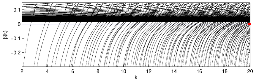
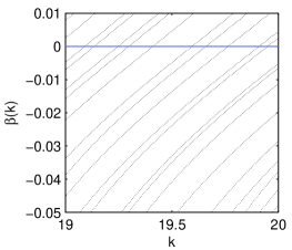
b) c) d)

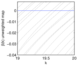
Figure 1. (a) Flow of the eigenvalues $\beta(k)$ of the weighted Neumann-to-Dirichlet map $\Theta$ vs wavenumber $k$, for the domain $\Omega$ given in polar coordinates by $r(\theta)=1+0.3\cos[3(\theta+0.2\sin\theta)]$. (b) Eigenmode $\phi_{93}$ (density shows absolute value; white is zero) with $k_{93}=19.94995891589\cdots$ (also shown by red dot in a). (c) Zoom in of flow. (d) Zoom in to the same region for eigenvalues of $\Lambda(k)^{-1}$ the unweighted Neumann-to-Dirichlet map; there is variation in slopes at the zero-crossings.

2. The Neumann-to-Dirichlet map and its spectral flow

We will use ${u}_{n}:=\partial_{n}u:=n\cdot\nabla u$ to denote the outward normal derivative of a function $u$ defined in $\overline{\Omega}$. Let $\Lambda(k)$ be the interior Dirichlet-to-Neumann operator for the Helmholtz equation with parameter $k^{2}$, that is, the operator that sends a function $g\in H^{1}({\partial\Omega})$ to the function $h\in L^{2}({\partial\Omega})$ given by $h={u}_{n}$, where $u$ is the interior Helmholtz extension satisfying

$$(\Delta+k^{2})u=0\quad\text{ in }\Omega,\qquad u|_{\partial\Omega}=g.$$ (3)

This is well defined for every $k\in{\mathbb{C}}$ except when $k=k_{j}$ is a Dirichlet eigenfrequency, in which case the function $u$ may not exist (and is nonunique when it does exist). It is well-known that for $k\neq k_{j}$, $\Lambda(k)$ is self-adjoint, as the following elementary calculation involving Green’s second identity shows. Suppose that $g,h\in H^{1}({\partial\Omega})$ and that $u,v$ are their interior Helmholtz extensions, respectively, then

$$\begin{gathered}\int_{\partial\Omega}\overline{(\Lambda g)}h-\int_{\partial\Omega}\overline{g}\Lambda h=\int_{\partial\Omega}{\overline{u}}_{n}v-\int_{\partial\Omega}\overline{u}{v}_{n}\\ =\int_{\Omega}[(\Delta+k^{2})\overline{u}]v-\overline{u}(\Delta+k^{2})v=0~{}.\end{gathered}$$

This and other properties of $\Lambda$ are presented by Friedlander [25].

Unless indicated, we work with a weighted inner product on the boundary ${\partial\Omega}$, denoted by angle brackets $\langle\cdot,\cdot\rangle$, and induced norm, as follows,

$$\langle g,h\rangle:=\int_{\partial\Omega}\overline{g(s)}h(s)\,\left(x(s)\cdot n(s)\right)^{-1}ds~{},\qquad\|g\|^{2}:=\langle g,g\rangle~{}.$$ (4)

Note that if $\Omega$ is strictly star-shaped about the origin, the weight is bounded and positive. It is easy to check that the operator $(x\cdot n)\circ\Lambda(k)$ is self-adjoint with respect to this weighted inner product. Let $\Theta(k)$ denote the inverse of this operator, that is, $\Theta(k):=\Lambda(k)^{-1}\circ(x\cdot n)^{-1}$, then $\Theta$ is also self-adjoint with respect to the weighted inner product. By definition, if $u$ is any interior Helmholtz solution, then

$$\Theta(k)\,(x\cdot n){u}_{n}=u|_{\partial\Omega}~{}.$$ (5)

In this paper, we will analyze the flow of eigenvalues and eigenspaces of $\Theta(k)$ as $k$ varies along the real axis, that is, nontrivial solutions $f\in{L^{2}({\partial\Omega})}$ to

$$\Theta(k)f(k)=\beta(k)f(k)~{}.$$ (6)

Taking $u=\phi_{j}$, a Dirichlet eigenmode, in (5), we see that $\Theta(k)$ has a zero eigenvalue at each Dirichlet eigenfrequency $k=k_{j}$, with eigenfunction $f=(x\cdot n)\partial_{n}\phi_{j}$; this is why the Neumann-to-Dirichlet map is of interest computationally. Considering the case of $u$ a Neumann Laplace eigenmode of the domain shows that $\Theta(k)$, and hence its spectrum, has a pole at each Neumann eigenfrequency $k$. Fig. 1 illustrates the zeros in $\beta(k)$ occurring at each of the lowest 93 Dirichlet eigenvalues of a domain (the poles are also hinted at for larger negative $\beta$). Also visible is the accumulation of eigenvalues at $0^{+}$ that occurs for all real $k$, a result of $\Lambda$ being a pseudodifferential operator of order $+1$ [25], hence $\Theta$ a compact operator (of order $-1$).

We wish to flow along an interval of the real $k$-axis that will likely contain several Neumann eigenfrequencies, and need to guarantee that all of the eigenprojections and eigenvalues of $\Theta$ vary smoothly except possibly for a finite number associated with a pole if $k$ is a Neumann eigenfrequency. To do that, we consider the Cayley transform of $\Theta$,

$$R(k)=\big{(}\Theta(k)-i\big{)}\big{(}\Theta(k)+i\big{)}^{-1}~{}.$$ (7)

In Appendix A, Corollary A.2, we show that $R(k)$ is analytic in some neighbourhood of the positive real axis. As $R(k)$ is unitary for real $k$, its spectrum lies on the unit circle, and is discrete except at $-1$ because $\Theta$ is compact (its spectrum accumulates only at $0$). Thus we deduce from Kato [34, Ch. VII, sec. 3] that the eigenprojections and eigenvalues of $R(k)$ vary analytically away from eigenvalue $-1$. Translated back to $\Theta$ this means that the eigenprojections and eigenvalues of $\Theta(k)$ vary analytically in $k$ on any finite $k$-interval away from eigenvalue $0$, apart from a finite number which have a pole at one of the Neumann eigenfrequencies in this interval.

Definition 2.1.

Let $\beta=\beta(k)$ be a finite eigenvalue of $\Theta(k)$ with boundary-normalized eigenfunction $f=f(k)$, $\|f\|=1$. The extended eigenfunction is then the unique solution $u$ to the interior boundary-value problem

$$(\Delta+k^{2})u = 0\quad\mbox{ \rm in }\Omega~{},$$ (8)

$$(x\cdot n){u}_{n} = f\quad\mbox{ \rm on }{\partial\Omega}~{},$$ (9)

$$u = \beta f\quad\mbox{ \rm on }{\partial\Omega}~{}.$$ (10)

Note that we have both Neumann and Dirichlet conditions on $u$; the latter is needed for uniqueness when $k$ is a Neumann eigenfrequency. Their consistency at all $k$ is ensured by (5). We may view $u$ as a solution to a Stekloff eigenvalue problem with Robin condition

$$\beta(x\cdot n){u}_{n}=u~{}.$$ (11)

Note that the extended eigenfunction $u$ is not normalized in ${L^{2}(\Omega)}$.

The rate of change with $k$ of each isolated eigenvalue is then given by the following variant of a result of Friedlander [25, Prop. 2.5]. For convenience we give the proof.

Lemma 2.2.

Let $\beta(k)$ be a analytic eigenvalue branch of $\Theta(k)$ with normalized eigenfunction $f=f(k)$, $\|f\|=1$, and let $u$ be its extended eigenfunction. Then, using the notation $\dot{\beta}:=d\beta(k)/dk$, it holds that

$$\dot{\beta}=2k\int_{\Omega}|u|^{2}~{}.$$ (12)

Proof.

From (6) follows the usual Hellman-Feynman formula,

$$\dot{\beta}=\frac{d}{dk}\langle\Theta f,f\rangle=\langle\dot{\Theta}f+\Theta\dot{f},f\rangle+\langle\Theta f,\dot{f}\rangle=\langle\dot{\Theta}f,f\rangle$$ (13)

where the last step comes from the normalization of $f$, which implies $\langle\dot{f},f\rangle=0$. Let $k=k_{0}$ be the frequency in the statement of the Lemma, and restrict for now to the case that this is not a Neumann eigenfrequency, in which case there is a unique solution $u$ to the pair (8) and (9) given boundary data $f$. Holding this boundary data fixed at $f=f(k_{0})$, let $v(k)$ be the solution to the boundary value problem

$$(\Delta+k^{2})v(k)=0,\quad(x\cdot n){v}_{n}(k)=f(k_{0}).$$ (14)

(Note $v$ is not the same as the extended eigenfunction $u$ except at $k=k_{0}$.) Let $\dot{v}$ be the $k$-derivative of this solution at $k=k_{0}$. Then, by the definition (5),

$$\dot{\Theta}f=\dot{v}|_{{\partial\Omega}}~{}\ \text{ at }k=k_{0}.$$ (15)

Also, by differentiating the defining conditions (14) we get a boundary value problem for $\dot{v}$,

$$(\Delta+k^{2})\dot{v}=-2kv\;\mbox{ in }\Omega,\qquad{\dot{v}}_{n}=0\;\mbox{ on }{\partial\Omega}.$$ (16)

Combining this with (15) and (13) in Green’s 2nd identity gives

$$\begin{gathered}\dot{\beta}(k_{0})=\langle\dot{\Theta}(k_{0})f,f\rangle=\int_{{\partial\Omega}}(x\cdot n)^{-1}\dot{\overline{v}}f=\int_{{\partial\Omega}}\dot{\overline{v}}{v}_{n}=\int_{{\partial\Omega}}\left(\dot{\overline{v}}{v}_{n}-{\dot{\overline{v}}}_{n}v\right)\\ =\int_{\Omega}\dot{\overline{v}}(\Delta+k_{0}^{2})v-[(\Delta+k_{0}^{2})\dot{\overline{v}}]v=2k_{0}\int_{\Omega}|v|^{2}=2k_{0}\int_{\Omega}|u|^{2}.\end{gathered}$$ (17)

This completes the proof when $k_{0}$ is not a Neumann eigenfrequency. When $k_{0}$ is a Neumann eigenfrequency, $f(k)$ and $\beta(k)$ are still analytic in a neighbourhood of $k_{0}$ (as discussed above), so one may take a sequence with $k_{0}$ as the limit and prove the same formula. ∎

This fact that this lemma can be applied in the limit $\beta\uparrow 0$ is justified at the end of App. A. Notice that we always have $\dot{\beta}>0$, illustrated by the positive slopes in Fig. 1.

We now can explain the reason for choosing the particular weight in the inner product (4). Let $\beta(k)$ be an analytic eigenvalue branch of $\Theta(k)$ which has $\beta(k_{j})=0$ for some $j$, that is, the branch corresponding to the $j$th eigenfrequency. Then at $k=k_{j}$, the extended eigenfunction $u$ is a Dirichlet eigenfunction. For Dirichlet eigenfunctions, we have Rellich’s identity [50] (a special case of (47)),

$$2k_{j}^{2}\int_{\Omega}|u|^{2}=\int_{{\partial\Omega}}(x\cdot n)|{u}_{n}|^{2}=\langle f,f\rangle=1~{}.$$ (18)

Inserting this into Lemma 12 gives a formula for the slopes at zero eigenvalue,

$$\beta=0\;\;\implies\;\;\dot{\beta}(k_{j})=\frac{1}{k_{j}}~{}.$$ (19)

Remark 2.3.

(19) shows that, for the special boundary weight function $(x\cdot n)^{-1}$, the eigenvalues of $\Theta(k)$ cross zero at a uniform, predictable positive speed that is independent of the details of the distribution of the eigenmode $\phi_{j}$. This predictable behavior is not known to occur for any other weight function: for example, the contrast between this special weight and the unweighted case (where speeds vary unpredictably with $j$) is shown in Fig. 1 (c) and (d).

3. Basic numerical algorithm

We first present a simple fast algorithm to approximate the eigenfrequencies and eigenfunctions of the domain $\Omega$ using spectral data of $\Theta$; in section 5 we will improve it to have higher-order accuracy.

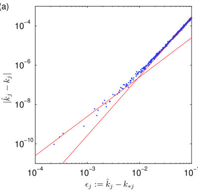
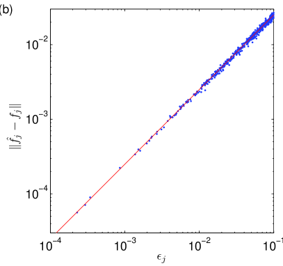
Figure 2. Errors with basic method, for the domain of Fig. 1(b). (a) Error of predicted eigenfrequency $\hat{k}_{j}$ using linear formula (20), vs prediction distance ${\epsilon}_{j}$, for all frequencies $k_{j}\in[90,100]$. Lines show $0.27{\epsilon}^{3}$ and $0.25{\epsilon}^{2}/k$. (b) Errors of predicted boundary functions $\hat{f}$ in the weighted $L^{2}$ norm (4). Line shows $0.25{\epsilon}$.

3.1. Reconstructing eigenfrequencies

Since each Dirichlet eigenfrequency $k_{j}$ is associated with an analytic eigenvalue branch of the spectrum of $\Theta(k)$, we may use this spectral flow of $\Theta(k)$ to locate approximately the $k_{j}$. Fig. 1 (c) illustrates that the gradients $\dot{\beta}(k)$ are approximately constant on each branch for $k$ near $k_{j}$; in section 4 we will prove that the range of $k_{j}-k$ for which this usefully holds is a constant independent of $k_{j}$. Thus, choosing a frequency $k_{*}$ and computing the spectrum of $\Theta(k_{*})$, then for each of its small negative eigenvalues $\beta_{*}=\beta(k_{*})$, one may extrapolate linearly to the corresponding Dirichlet eigenvalue by the

$$\mbox{``linear estimator'':}\qquad\hat{k}\;=\;\frac{k_{*}}{1+\beta_{*}}~{}.$$ (20)

This follows simply from (19) and by making the linear approximation $\beta_{*}\approx\dot{\beta}(k_{j})(k_{*}-k_{j})$. We keep only those $\hat{k}$ values lying in the interval or ‘window’ $[k_{*},k_{*}+{\epsilon}]$, where ${\epsilon}$ is an $O(1)$ constant. Since, by Weyl’s law [26, Ch. 11] asymptotically $O(k^{d-1})$ eigenfrequencies lie in such an interval, this is also the order by which the method is faster than the standard iterative search for each eigenfrequency. By repeating the above with adjacent intervals one may find approximations to all eigenfrequencies lying in any desired subset of the frequency axis.

In section 3.3 we present the spectrally-accurate method we use (in $d=2$) to compute numerically the spectrum of $\Theta(k_{*})$. This algorithm has been built into the MPSpack toolbox toolbox for MATLAB [54], so that the set of approximate eigenfrequencies $\hat{k}_{j}$ lying in $[90,100]$ may be computed, for example, for the nonsymmetric, smooth (in fact analytic) domain $\Omega\subset{\mathbb{R}}^{2}$ shown in Fig. 1 (b), as follows:

s = segment.smoothnonsym(720, 0.3, 0.2, 3); % create a closed curve
d = domain(s, 1);                           % create an interior domain
s.setbc(-1, ’D’);                           % Dirichlet BCs on inside
p = evp(d);                                 % create eigenvalue problem
o.khat = ’l’; o.eps = 0.1; p.solvespectrum([90 100], ’ntd’, o);

Here $N=720$ sets the number of boundary quadrature points to about 6 per wavelength on the boundary, typically sufficient for approximating $\Theta$ at close to double-precision accuracy. The options structure o chooses the linear method (20) and sets ${\epsilon}=0.1$. The object p now contains p.kj, being the list of 492 approximate eigenfrequencies $\hat{k}_{j}$ found (these are in fact numbers $j=[2064,2555]$ for the domain). All were found to be simple, as expected generically since $\Omega$ has no symmetry. The majority of them have absolute errors less than $10^{-4}$. The CPU time for the above example was 13 min, ie 1.6 s per computed eigenfrequency.

The size of the absolute eigenfrequency errors are shown in Fig. 2 (a), versus

$${\epsilon}_{j}:=k_{j}-k_{*}~{},$$ (21)

the frequency ‘distance’ over which the linearization occurred. Errors are $O({\epsilon}_{j}^{2}/k)$ at small distances but $O({\epsilon}_{j}^{3})$ at large distances: these two terms are shown by straight lines in Fig. 2 (a). We are able to prove a bound involving these two terms in Corollary 4.2, which states that the implied constants are independent of $k$. The transition point (intersection of the straight lines) occurs at ${\epsilon}=O(1/k)$. Since generically only a fraction $O(1/k)$ of the eigenfrequencies in the window lie below this ${\epsilon}$ distance, the method is asymptotically 3rd-order accurate in the interval width ${\epsilon}$.

These errors reported above were found by comparison against an accurate set of eigenfrequencies $k_{j}$ found independently by a standard method from the literature described in App. B. This reference method requires 53 s per eigenfrequency found, thus our method is a factor 33 times faster. Assuming constant absolute eigenfrequency error is acceptable, then this speed-up factor grows (in $d=2$) in proportion to $O(N)=O(k)$: the reference method takes $O(N^{3})$ effort per eigenfrequency found whereas our proposed method takes only $O(N^{2})$ effort.

3.2. Reconstructing eigenfunctions from boundary data

We assume for now that for each eigenvalue $\beta_{*}$ of $\Theta(k_{*})$ we can generate an accurate approximation to its corresponding boundary eigenfunction $f_{*}$ (e.g. as in section 3.3). Approximations $\hat{\phi}$ to Dirichlet eigenfunctions $\phi_{j}$ can then be evaluated using potential theory, as follows.

At wavenumber $k$, the free space Green’s function for the Helmholtz equation, $G_{0}(k;x,y)$, is defined as the unique radiating solution to $-(\Delta+k^{2})G_{0}=\delta$ in ${\mathbb{R}}^{d}$, where $\delta$ is the Dirac delta distribution. Specifically, we have,

$$G_{0}(k;x,y)=\frac{i}{4}\biggl{(}\frac{k}{2\pi|x-y|}\biggr{)}^{d/2-1}\!\!H_{d/2-1}^{(1)}(k|x-y|),\qquad x,y\in{\mathbb{R}}^{d},$$ (22)

where $H_{\nu}^{(1)}$ is the outgoing Hankel function of order $\nu$ [46, Ch. 10]. The standard single- and double-layer potentials [18] are then defined for $x\in\Omega$ by

$$({\mathcal{S}}(k)\sigma)(x) = \int_{\partial\Omega}G_{0}(k;x,y)\sigma(y)ds_{y}~{},$$ (23)

$$({\mathcal{D}}(k)\tau)(x) = \int_{\partial\Omega}\frac{\partial G_{0}(k;x,y)}{\partial n_{y}}\tau(y)ds_{y}~{},$$ (24)

where the derivative is with respect to the $y$ variable in the outward surface normal direction at $y$. Then any solution $u$ to $(\Delta+k^{2})u=0$ in $\Omega$ with smooth boundary may be written via Green’s representation theorem [18],

$$u={\mathcal{S}}(k)u_{n}-{\mathcal{D}}(k)u|_{\partial\Omega}\quad\mbox{ in }\Omega~{}.$$ (25)

Suppose an exact eigenfrequency $k_{j}$ were known, and also $f_{j}=f(k_{j})$ the corresponding exact eigenfunction of $\Theta(k_{j})$. We could then use (25) to compute the extended eigenfunction $u_{j}$, since its Dirichlet data vanishes, and its Neumann data is given by (9). According to (18) we also need a prefactor $\phi_{j}=\sqrt{2}k_{j}\,u_{j}$ to recover unit ${L^{2}(\Omega)}$ norm. Thus a Dirichlet eigenfunction $\phi_{j}$ is represented exactly throughout $\Omega$ by

$$\phi_{j}=\sqrt{2}k_{j}\,{\mathcal{S}}(k_{j})[(x\cdot n)^{-1}f_{j}]~{}.$$ (26)

However, we do not have access to $f_{j}$; we only have $f_{*}$, the corresponding eigenfunction of $\Theta(k_{*})$ for $k_{*}$ near $k_{j}$. Similarly, $k_{j}$ is only known approximately (e.g. as in the previous section). Given approximations $\hat{k}\approx k_{j}$ and $\hat{f}\approx f_{j}$, we propose to reconstruct an approximate eigenfunction via

$$\hat{\phi}=\sqrt{2}\hat{k}\,{\mathcal{S}}(\hat{k})[(x\cdot n)^{-1}\hat{f}]~{}.$$ (27)

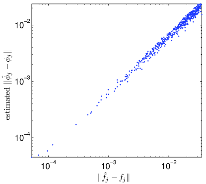
Figure 3. Scatter plot of estimated eigenfunction errors in the ${L^{2}(\Omega)}$ norm versus corresponding boundary function $f$ errors in the weighted ${L^{2}({\partial\Omega})}$ norm, for the domain of Fig. 1 and $k_{j}\in[90,100]$ with the basic method. ${L^{2}(\Omega)}$ norms are estimated on a Cartesian grid of 327 interior points, giving a statistical error of order $\pm 10\%$.

For now we will present a method that is only first-order in ${\epsilon}$: we use the

$$\mbox{``trivial $f$ estimator'':}\qquad\hat{f}=f_{*}~{}.$$ (28)

(We present higher-order methods in section 5.) Figure 2(b) shows the resulting $\|\hat{f}-f_{j}\|$ errors in the weighted ${L^{2}({\partial\Omega})}$ norm, computed relative to a highly-accurate set of boundary functions $f_{j}$ found by the method of App. B. This behavior is clearly first order.

Remark 3.1.

To prove a rigorous estimate on $\|\hat{f}-f_{j}\|$ one would need to control $\dot{f}$ over the interval $[k_{*},k_{j}]$; we have by (74) and Lemma 4.4 that $\|\dot{f}\|=O(1)$ at $k=k_{j}$, but cannot exclude the possibility that “avoided crossings” in the spectral flow cause $\dot{f}$ to be much larger at other $k$ values. Based on empirical observations, the latter possibility seems very rare.

How do the errors in $\hat{f}$ propagate to errors in eigenfunctions $\hat{\phi}$? To test this, we insert $\hat{f}=f_{*}$, and $\hat{k}$ from (20), into the reconstruction formula (27), and estimate numerically the ${L^{2}(\Omega)}$ errors against an accurate set of reference eigenfunctions $\phi_{j}$. In the resulting Fig. 3 the data clusters close to a straight line of unit slope (scatter from this line being part due to our estimation of ${L^{2}(\Omega)}$ errors using a relatively small number of interior points). Hence the domain error norm of $\phi$ is empirically controlled by the boundary error norm of $f$. This is to be expected because, although (26) and (27) use different wavenumbers, the error in $\hat{k}$ is of higher order than that of $\hat{f}$, and error induced by the $k$-dependence of ${\mathcal{S}}(k)$ is expected to be negligible.

Remark 3.2.

Supported by the above evidence, we henceforth discuss eigenfunction errors only in terms of boundary functions $f$, postponing analysis of $\|\hat{\phi}-\phi_{j}\|_{{L^{2}(\Omega)}}$ to future work. A rigorous proof that boundary error controls domain error would demand bounds on the $k$-dependence of the operator ${\mathcal{S}}(k):{L^{2}({\partial\Omega})}\to{L^{2}(\Omega)}$. Accurate numerical study of ${L^{2}(\Omega)}$ errors is also difficult, since i) the eigenmodes are highly oscillatory, demanding $O(k^{2})$ evaluation points (in the above example around $10^{5}$ would be needed), and ii) accurate evaluation of a layer potential such as (27) near ${\partial\Omega}$ is difficult and a topic of current research [31].

In terms of computational effort, extracting all boundary eigenfunctions $f_{*}$ at each $k_{*}$ is best done by complete diagonalization of a matrix (given below by (44)) at each $k_{*}$; this increases the CPU time per mode from the 1.6 s of the previous section (when only matrix eigenvalues were needed) to around 2.3 s per mode. However, the reference method of App. B also requires longer to extract modes (an additional 14 s per mode). The net effect is that the proposed NtD method is still 30 times faster than the reference method.

Remark 3.3.

In [12] we proved error bounds on $\hat{k}$ and on the ${L^{2}(\Omega)}$ error of $\hat{\phi}$ in terms of $\|\hat{\phi}\|_{L^{2}({\partial\Omega})}$. The latter could be evaluated using (27) and a singular quadrature scheme as in Section 3.3. This would remove any need to compare against reference eigenpairs. However, we avoided this approach since the errors in $f$ would dwarf the higher-order errors in $k$ that we wish to study.

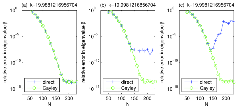
Figure 4. Convergence of numerical scheme for eigenvalues $\beta$ of $\Theta(k)$ at three different $k$ values with distances from a Neumann eigenfrequency as follows: (a) $10^{-2}$, (b) $10^{-10}$, (c) zero. The domain is as in Fig. 1. The $\beta$ tested was the largest negative eigenvalue (i.e. closest to zero), roughly $-5\times 10^{-3}$ in each case. The proposed Cayley scheme (36) and (37) is compared against the direct discretization of (38).

3.3. Numerical computation of spectrum of $\Theta$

To implement the above algorithm, at any given frequency $k$ we need to compute numerical approximations to an $O(1)$ fraction of the eigenpairs of the weighted NtD operator $\Theta(k)$. Here we present, and test, a robust integral equation method based upon the Cayley transform. We need some standard results from potential theory [18]. Let $S(k)$ and $D(k)$ be the single- and double-layer boundary integral operators formed by restricting (23) and (24) respectively to the boundary,

$$(S(k)\sigma)(x) = \int_{\partial\Omega}G_{0}(k;x,y)\sigma(y)ds_{y}~{},\qquad x\in{\partial\Omega}$$ (29)

$$(D(k)\tau)(x) = \int_{\partial\Omega}\frac{\partial G_{0}(k;x,y)}{\partial n_{y}}\tau(y)ds_{y}~{}.\qquad x\in{\partial\Omega}$$ (30)

Then, taking $x\in\Omega$ to the boundary in the representation formula (25), and applying the jump relation for the double layer potential,

$$({\mathcal{D}}\tau)\big{|}_{{\partial\Omega}}=(D-\mbox{\small$\frac{1}{2}$})\tau~{},$$ (31)

gives, for any Helmholtz solution $(\Delta+k^{2})u=0$ in $\Omega$, the boundary data relation

$$(\mbox{\small$\frac{1}{2}$}+D)u|_{\partial\Omega}=Su_{n}~{}.$$ (32)

We also record for later use the jump relation for the single layer potential,

$${({\mathcal{S}}\sigma)}_{n}=(D^{t}+\mbox{\small$\frac{1}{2}$})\sigma~{}.$$ (33)

We now generalize the Cayley transform (7) slightly, defining

$$R_{\eta}(k):=\big{(}\eta\Theta(k)-i\big{)}\big{(}\eta\Theta(k)+i\big{)}^{-1}~{},$$ (34)

where $\eta\in{\mathbb{R}}\setminus\{0\}$ is a scale parameter with units of inverse length (i.e. of $k$). Therefore, if $R_{\eta}(k)f=g$, we have

$$\big{(}\eta\Theta+i\big{)}g=\big{(}\eta\Theta-i\big{)}f,$$

which we rearrange to

$$\Theta[i\eta(g-f)]=g+f~{}.$$

That is, there exists a function $u$ on $\Omega$ such that

$$\big{(}\Delta+k^{2})u=0,\quad u_{n}=i\eta(x\cdot n)^{-1}(g-f),\quad u|_{\partial\Omega}=g+f.$$ (35)

Inserting this boundary data into (32) implies

$$i\eta S[(x\cdot n)^{-1}(g-f)]=(\mbox{\small$\frac{1}{2}$}+D)(g+f)$$

which can be rearranged, recalling that $R_{\eta}f=g$ for all $f$, to show,

$$R_{\eta}=({K}_{-})^{-1}{K}_{+},\quad{K}_{\pm}=\pm(\mbox{\small$\frac{1}{2}$}+D)+i\eta S\circ(x\cdot n)^{-1}~{}.$$ (36)

The scheme is now to choose the scale parameter (we prefer $\eta=k$, similar to [36]), and to approximate the spectrum and eigenfunctions of $R_{\eta}$, using known efficient Nyström discretizations for the operators $S$ and $D$, as described below. We then convert back to eigenpairs of $\Theta$ as follows: the eigenvalues $\beta$ of $\Theta$ come from the eigenvalues $\lambda$ of $R_{\eta}$ simply by inverting the formula (34), that is,

$$\beta=\frac{i}{\eta}\frac{1+\lambda}{1-\lambda}~{},$$ (37)

and the eigenfunctions of $\Theta$ are the same as those of $R_{\eta}$.

Remark 3.4.

The advantage of discretizing (36) then transforming eigenvalues via (37), over discretizing the usual direct representation of the weighted NtD map

$$\Theta=(\mbox{\small$\frac{1}{2}$}+D)^{-1}S\circ(x\cdot n)^{-1}$$ (38)

which follows from (32), is that $R_{\eta}(k)$ is unitary and thus its eigenvalues remain of size $O(1)$. By contrast, the eigenvalues of $\Theta(k)$ have a large dynamic range, and a finite number of eigenvalues diverge to infinity whenever $k$ is a Neumann eigenfrequency of the domain, causing inevitable large round-off error in the desired (small) eigenvalues. We demonstrate this contrast numerically in Fig. 4: in the ‘direct’ method this round-off error limits accuracy in $\beta$ to 8 digits for $k$ near a Neumann eigenfrequency (and fails to converge at a Neumann eigenfrequency), whereas the ‘Cayley’ method achieves 14-digit accuracy uniformly in $k$. (Note that we expect some mild loss of accuracy as $k$ increases, due to the condition number of the $({K}_{-})^{-1}$ factor, but in the range explored in this paper, $1<k<10^{3}$, this was negligible.) Thus to discretize (38) is not robust, whereas our proposed scheme is robust.

We summarize briefly our preferred Nyström discretization for Helmholtz layer potential operators on analytic curves in $d=2$, following Kress [36]. Let $z:[0,2\pi)\to{\mathbb{R}}^{2}$ be a $2\pi$-periodic parametrization of ${\partial\Omega}$, and let $k(x,y)$ be the kernel of either $S$ or $D$. Changing variable to $s,t\in[0,2\pi)$ we get kernel $K(s,t):=k(z(s),z(t))|z^{\prime}(t)|$ where $z^{\prime}=dz/dt$. Note that $S$ has a logarithmic singularity on its diagonal, whereas $D$ has a continuous kernel but is non-analytic on the diagonal; in both cases the following splitting allows spectral accuracy to be achieved. We choose quadrature nodes $t_{j}=2\pi j/N$, $j=1,\ldots,N$, and split the kernel into the form

$$K(s,t)=\log\left(4\sin^{2}\frac{s-t}{2}\right)K_{1}(s,t)+K_{2}(s,t)$$ (39)

with $K_{1}$ and $K_{2}$ both $2\pi$-periodic and analytic. The matrix representation of $K_{2}$ comes from the periodic trapezoid rule (weights being constant at $2\pi/N$), whereas the representation of $K_{1}$ involves a product quadrature appropriate for the periodized log singularity. Together these give a matrix ${\mathbf{K}}$ with elements

$${\mathbf{K}}_{ij}=\frac{2\pi}{N}\left[R^{(N)}_{|i-j|}(0)\,K_{1}(t_{i},t_{j})+K_{2}(t_{i},t_{j})\right],\quad i,j=1,\ldots,N~{},$$ (40)

where the Martensen–Kussmaul quadrature weights (deriving from the Fourier series for the log factor, see [37, Lemma 8.21]) are defined by

$$R^{(N)}_{j}(s)\;=\;-\sum_{m=1}^{N/2-1}\frac{2}{m}\cos m(s-t_{j})\;-\;\frac{2}{N}\cos\frac{N}{2}(s-t_{j})~{}.$$ (41)

Abusing notation slightly by letting $K$ be an operator with kernel $K(s,t)$, it is standard to approximate operator eigenvalue problems of the type

$$K\phi=\lambda\phi$$ (42)

by the $N$-dimensional matrix eigenvalue problem

$${\mathbf{K}}\phi^{(N)}=\lambda^{(N)}\phi^{(N)}~{}.$$ (43)

If $K$ were compact and normal, it is known that the spectrum and eigenspaces of (43) converge to those of (42) as $N\to\infty$ [2], at a rate given by the error of the quadrature scheme applied to vectors in the eigenspace (for the spectrum see [3]—here normality ensures that the index of each eigenvalue is one—and for the eigenspaces see [47, Thm. 1]). This analysis relies on the framework of collectively compact operators [1] [37, Ch. 10]. The above product quadrature scheme is within this framework and is spectrally accurate for analytic functions, i.e. errors are bounded by $ce^{-\gamma N}$ for some $\gamma>0$ [36, 37].

However, our goal is to approximate the spectrum and eigenspaces of the operator $R_{\eta}$; this is not covered by the above-mentioned analytic results, for two reasons. Firstly $R_{\eta}$ is not compact (although $R_{\eta}+I$ is), and secondly the application of $R_{\eta}$ in (36) requires an operator product and inverse. We will not attempt a rigorous error analysis here, rather merely describe our scheme and show its efficacy. We approximate the spectrum of $R_{\eta}$ by that of the matrix

$${\mathbf{R}}_{\eta}=({\mathbf{K}}_{-})^{-1}{\mathbf{K}}_{+}$$ (44)

built from the matrices ${\mathbf{K}}_{\pm}$ which approximate the operator factors $K_{\pm}$ appearing in (36), according to the above Nyström scheme (40). Dense linear algebra is used both for the matrix inverse ${\mathbf{K}}_{-}^{-1}$ in (36), and the full diagonalization of ${\mathbf{R}}_{\eta}$ (MATLAB’s inv and eig respectively). The computational effort is $O(N^{3})$. The eigenvectors of ${\mathbf{R}}_{\eta}$ then give approximations to the eigenvectors of $R_{\eta}$, hence of $\Theta$, at the quadrature nodes. In MPSpack the above algorithm is available via

[beta,V] = p.NtDspectrum(k);

which returns approximate eigenvalues of $\Theta(k)$ in beta, and corresponding eigenfunction values at the quadrature points in the columns of V. Returning to Fig. 4 we observe exponential convergence of this ‘Cayley’ scheme, with saturation at relative error $10^{-14}$ uniformly in $k$.

4. Error analysis of the linear eigenfrequency estimator

The main result of this section is an estimate on the accuracy of the eigenfrequencies as reconstructed by the basic formula (20). In section 5.1 we will describe an improved method for which we can prove better error estimates, but those better estimates are conditional on absence of spectral concentration (Assumption 6.1); here, the result is unconditional.

The key result is the following bound on the deviation from linearity of the weighted NtD eigenvalue flow.

Theorem 4.1.

There are constants $\epsilon,K>0$ dependent only on $\Omega$ such that the following holds. Let $k_{p}>K$ be a Dirichlet eigenfrequency, and $\beta(k)$ be the corresponding eigenvalue branch of $\Theta(k)$, i.e. such that $\beta(k_{p})=0$ (the existence of which is guaranteed by Proposition A.5). Then

$$\beta(k)=\frac{k-k_{p}}{k_{p}}+O\Big{(}\frac{(k-k_{p})^{2}}{k_{p}^{2}}+\frac{(k-k_{p})^{3}}{k_{p}}\Big{)}$$ (45)

for all $k\in[k_{p}-{\epsilon},k_{p}]$. The implied constant in the $O(\cdot)$ depends only on $\Omega$.

It is then easy to derive the following error estimate for the basic method. Note that we have already numerical evidence (section 3.1) that the powers of ${\epsilon}$ are sharp.

Corollary 4.2.

There are constants $\epsilon,C>0$ depending only on $\Omega$ such that, for any sufficiently large $k_{*}$, and any $k_{p}$ lying in the range $[k_{*},k_{*}+{\epsilon}]$, and $\beta(k)$ related to $k_{p}$ as in Theorem 4.1, we have

$$|\hat{k}-k_{p}|\;\leq\;C\Big{(}\frac{\epsilon^{2}}{k_{*}}+\epsilon^{3}\Big{)}$$ (46)

where $\hat{k}=k_{*}/(1+\beta(k_{*}))$ is the linear estimator of $k_{p}$ according to (20).

Remark 4.3.

Note that the theorem holds for a fixed window width ${\epsilon}$, independent of $k$. By Weyl’s Law there are $O(k^{d-1})$ eigenfrequencies lying in such a window; all are found within the stated error. As $k$ grows, the $\epsilon^{2}/k$ term becomes negligible for almost all reconstructed eigenfrequencies, thus the eigenfrequency error of the basic method is effectively $O({\epsilon}^{3})$ with constant independent of $k$.

Proof of Theorem 4.1. We use the following identity from [9, Lemma 3.1], which allows one to express the right hand side of (12) in terms of boundary data: for any Helmholtz solution $u$ at frequency $k$, we have

$$2k^{2}\int_{\Omega}|u|^{2}=\int_{{\partial\Omega}}(x\cdot n)\big{(}|u_{n}|^{2}+k^{2}|u|^{2}-|\nabla_{\mbox{\rm\tiny tan}}{u}|^{2}\big{)}+{u}_{n}\overline{Wu}+(Wu)\overline{{u}_{n}}.$$ (47)

Here, $\nabla_{\mbox{\rm\tiny tan}}{}$ is the tangential gradient on ${\partial\Omega}$, and $W$ is the tangential part of the vector field $x\cdot\nabla$ which generates dilations. Explicitly, $W=x_{\mbox{\rm\tiny tan}}\cdot\nabla_{\mbox{\rm\tiny tan}}{}$ where $x_{\mbox{\rm\tiny tan}}=x-(x\cdot n)n$. For example, in $d=2$ we have $\nabla_{\mbox{\rm\tiny tan}}{=}\partial_{t}$ and $W=(x\cdot t)\partial_{t}$, where $t$ is the unit tangent vector. Putting (47) together with (12), taking $u$ to be the extended eigenfunction, we obtain

$$\dot{\beta}(k)=\frac{1}{k}\bigg{(}\int_{{\partial\Omega}}(x\cdot n)\big{(}|{u}_{n}|^{2}+k^{2}|u|^{2}-|\nabla_{\mbox{\rm\tiny tan}}{u}|^{2}\big{)}+2\operatorname{Re}({u}_{n}\overline{Wu})\bigg{)}.$$ (48)

The principal term on the right hand side of (48) is (using 18),

$$\frac{1}{k}\int_{{\partial\Omega}}(x\cdot n)|{u}_{n}|^{2}=\frac{1}{k}\|f\|^{2}=\frac{1}{k}.$$

The other terms are small when $\beta$ is small, and we try to estimate them in terms of $\beta$. Two of the terms are not hard to estimate: we have using the boundary condition (11),

$$\int_{{\partial\Omega}}(x\cdot n)k^{2}|u|^{2}=O(\beta^{2}k^{2}),$$

while (using the divergence theorem on ${\partial\Omega}$ in the third step below),

$$\int_{{\partial\Omega}}2\operatorname{Re}((Wu)\overline{{u}_{n}}) = \int_{{\partial\Omega}}(x\cdot n)^{-1}\beta^{-1}\cdot 2\operatorname{Re}((Wu)\overline{u})$$

$$= \frac{1}{\beta}\int_{{\partial\Omega}}(x\cdot n)^{-1}W(|u|^{2})$$

$$= -\frac{1}{\beta}\int_{{\partial\Omega}}|u|^{2}(W+\operatorname{div}W)(x\cdot n)^{-1}$$

$$= -\beta\int_{{\partial\Omega}}\big{(}(x\cdot n)W((x\cdot n)^{-1})+\operatorname{div}W\big{)}(x\cdot n)|{u}_{n}|^{2}$$

$$= O(\beta).$$

The scalar function $\operatorname{div}W$ may also be written $\nabla_{\mbox{\rm\tiny tan}}{}\cdot x_{\mbox{\rm\tiny tan}}$. To deal with the $|\nabla_{\mbox{\rm\tiny tan}}{u}|^{2}$ term in (48), we prove the following in Appendix C:

Lemma 4.4.

There are constants $c$, $K>0$ depending only on $\Omega$, such that whenever $k\geq K$ and $u$ solves $(\Delta+k^{2})u=0$ in $\Omega$, with

$$u=\beta(x\cdot n){u}_{n}\quad\text{ on }{\partial\Omega}$$ (49)

for some Robin constant $\beta\in[-c,0]$, then

$$\|\nabla_{\mbox{\rm\tiny tan}}{u}\|_{L^{2}({\partial\Omega})}\leq 2k\|u\|_{L^{2}({\partial\Omega})}.$$ (50)

Remark 4.5.

The intuition behind Lemma 4.4 is that $f$, as a boundary trace of a Helmholtz solution at frequency $k$, should be band-limited to frequencies $\leq k$. Indeed, the coefficient $2$ in (50) could be replaced by any factor $\alpha$ strictly larger than $1$, for $k\geq K(\alpha)$. Also, using the same proof is not hard to show the corresponding result for higher derivatives:

$$\|\nabla^{(m)}_{\tan}u\|_{L^{2}({\partial\Omega})}\leq 2k^{m}\|u\|_{L^{2}({\partial\Omega})},\quad k\geq K_{m}~{}.$$ (51)

Using Lemma 4.4, we can estimate the $|\nabla_{\mbox{\rm\tiny tan}}{u}|^{2}$ term in (47) the same way as the $k^{2}u^{2}$ term. So, combining the estimates of terms in (48), we get

$$\dot{\beta}(k)=\frac{1}{k}+O\Big{(}\frac{|\beta|}{k}\Big{)}+O(\beta^{2}k)\quad\mbox{whenever }-c\leq\beta\leq 0~{},$$ (52)

with implied constants depending only on $\Omega$.

We now conclude the proof of Theorem 4.1 by establishing (45). This follows directly from (54) below by integrating in $k$. Therefore, it remains to prove the following result:

Lemma 4.6.

There exists constants ${\epsilon},C_{1}>0$ depending only on $\Omega$ such that, for any sufficiently large $k_{p}$ (with $\beta(k)$ as in Theorem 4.1), it holds for all $k\in[k_{p}-{\epsilon},k_{p}]$ that

$$\frac{2(k-k_{p})}{k_{p}}\leq\beta(k)\leq\frac{k-k_{p}}{2k_{p}}~{},\quad\text{and}$$ (53)

$$\Big{|}\dot{\beta}(k)-\frac{1}{k_{p}}\Big{|}\leq C_{1}\Big{(}\frac{k_{p}-k}{k_{p}^{2}}+\frac{(k_{p}-k)^{2}}{k_{p}}\Big{)}~{}.$$ (54)

Proof.

We first prove the left hand side of (53). We first use the continuity of $\beta(k)$ to observe that in some small left neighbourhood $(k^{\prime\prime},k_{p}]$ of $k_{p}$, $\beta(k)$ itself is arbitrarily close to $0$ — in particular, such that $\beta(k)\geq-c$. Therefore, (52) applies, and, by requiring $\beta$ sufficiently small we can make the right hand side of (52) less than $3/(2k)$, and hence less than $2/k_{p}$ (since $k/k_{p}$ can be made as close as we like to $1$). By integrating this, we find that in this neighbourhood we have the left hand inequality in (53). However, the size of the neighbourhood may still depend on $k_{p}$.

Now we prove that for some $\epsilon>0$, the left hand inequality in (53) holds on each interval $[k_{p}-\epsilon,k_{p}]$ for all sufficiently large $k_{p}$. We do this by contradiction. Suppose that there is a $k\in[k_{p}-\epsilon,k_{p}]$ such that $\beta(k)<2(k-k_{p})/k_{p}$. Let $k^{\prime}$ be the largest such element of the interval $[k_{p}-\epsilon,k_{p}]$; notice that $k^{\prime}$ is strictly less than $k_{p}$ using the paragraph above. Then we have

$$\beta(k)\geq 2\frac{k-k_{p}}{k_{p}}\text{ for }k\in[k^{\prime},k_{p}],\quad\beta(k^{\prime})=2\frac{k^{\prime}-k_{p}}{k_{p}}.$$ (55)

For small $\epsilon$ relative to $k$ this certainly implies that $\beta\geq-c$ on the interval $[k^{\prime},k_{p}]$, so (52) applies. Using (52) and the estimate (55) we find that

$$\dot{\beta}(k) \leq\frac{1}{k}+C\Big{(}\frac{2(k_{p}-k)}{kk_{p}}+\frac{4k(k_{p}-k)^{2}}{k_{p}^{2}}\Big{)},\quad k\in[k^{\prime},k_{p}]$$ (56)

$$\leq\frac{1}{k}\bigg{(}1+C\Big{(}\frac{2\epsilon}{k_{p}}+\frac{4\epsilon^{2}k^{2}}{k_{p}^{2}}\Big{)}\bigg{)}$$

$$\leq\frac{3}{2k}$$

$$\leq\frac{1.6}{k_{p}},$$

where we need $\epsilon$ sufficiently small in the second last line, and $k_{p}$ sufficiently large in the last. Integrating this we find that

$$\beta(k_{p})-\beta(k^{\prime})\leq\frac{1.6(k_{p}-k^{\prime})}{k_{p}},$$

which contradicts the second part of (55). We conclude that no such $k^{\prime}$ exists, so the left hand inequality of (53) holds on the whole interval $[k_{p}-\epsilon,k_{p}]$.

The right hand inequality is proved similarly. In fact, using the left hand inequality, we see for small $\epsilon$ that $\beta\geq-c$ on the whole interval $[k_{p}-\epsilon,k_{p}]$, so we can use (52) on the whole interval, and conclude in a similar way to (56) that

$$\dot{\beta}(k)\geq\frac{0.8}{k_{p}},\quad k\in[k_{p}-\epsilon,k_{p}]$$

to derive the right hand inequality in (53).

To prove (54), we first note that (53) inserted into (52) implies that

$$\Big{|}\dot{\beta}(k)-\frac{1}{k}\Big{|}\leq C_{1}\Big{(}\frac{k_{p}-k}{kk_{p}}+\frac{k(k_{p}-k)^{2}}{k_{p}^{2}}\Big{)},\quad k\in[k_{p}-\epsilon,k_{p}].$$ (57)

This is almost the same as (54), but there are factors of $k$ in place of $k_{p}$. For the left hand side, replacing $1/k$ by $1/k_{p}$ makes an error of $(k_{p}-k)/kk_{p}$, and this can be absorbed on the right hand side (by increasing $C_{1}$ by $1$). Then, by taking $k_{p}$ large relative to $\epsilon$, we can replace the occurrences of $k$ on the right hand side by $k_{p}$, at the cost of increasing $C_{1}$ slightly. We conclude that (54) holds. ∎

Remark 4.7.

Theorem 4.1 and Corollary 4.2 imply that every $k_{p}$ slightly bigger than $k_{*}$ corresponds to a slightly negative eigenvalue $\beta$ of $\Theta(k_{*})$, with an almost linear relationship between $k_{p}$ and $\beta$. The converse is also true: every slightly negative eigenvalue $\beta$ of $\Theta(k_{*})$ corresponds to a $k_{p}$ slightly bigger than $k_{*}$. To see this we note that (52), and Proposition A.5, imply that the eigenvalue branch starting at $\beta(k_{*})\geq-\epsilon/k$ will, for small $\epsilon$, reach zero near $k\approx k_{*}/(1+\beta(k_{*}))$. Thus there is a one-to-one correspondence between eigenfrequencies $k_{p}$ slightly bigger than $k_{*}$, and the slightly negative eigenvalues of $\Theta(k_{*})$.

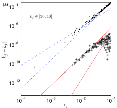
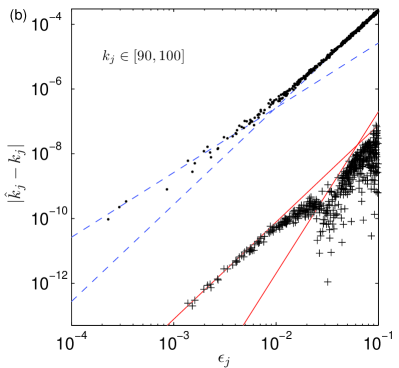
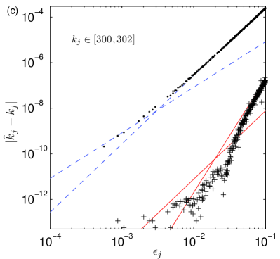
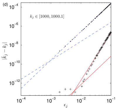
Figure 5. Errors of the two eigenfrequency prediction schemes for four different $k$ ranges, vs ${\epsilon}_{j}:=k_{j}-k_{*}$. Linear scheme (dots), using (20), compared against power laws $0.27\varepsilon^{3}$ and $0.25\varepsilon^{2}/k$ (dotted lines). Higher-order Riccati scheme (crosses), using (65), compared against $0.02\varepsilon^{5}$ and $7\varepsilon^{3}/k^{2}$ (solid lines). For the power laws, the mean $k$ in the interval is used. The domain is as in Fig. 1(b).

5. Higher-order accurate reconstruction methods

5.1. Higher-order eigenfrequency approximation

In section 3.1 we presented a formula (20) for eigenfrequencies $k_{p}$. For its error analysis in section 4 we treated all terms on the right hand side of (48), other than the first, as error terms, and estimated them. However, numerically we have at our disposal not just the eigenvalues of $\Theta(k_{*})$, but the eigenfunctions. Observe that the RHS of (48) can be expressed exactly in terms of $\beta$ and its associated eigenfunction $f$, using the relation $u|_{{\partial\Omega}}=\beta f$ from (10). Precisely, we have

$$k^{2}\int_{{\partial\Omega}}(x\cdot n)|u|^{2}=k^{2}\beta^{2}\|(x\cdot n)f\|_{{\partial\Omega}}^{2},$$ (58)

$$\int_{{\partial\Omega}}(x\cdot n)|\nabla_{\tan}u|^{2}=\beta^{2}\|(x\cdot n)\nabla_{\tan}f\|_{{\partial\Omega}}^{2},$$ (59)

$$\int_{{\partial\Omega}}2(x\cdot n)\operatorname{Re}({u}_{n}\overline{Wu})=-\beta\int_{{\partial\Omega}}(W+\operatorname{div}W)((x\cdot n)^{-1})|f|^{2}=-\beta\langle f,mf\rangle~{},$$ (60)

where we introduce the scalar boundary function

$$m:=(x\cdot n)W((x\cdot n)^{-1})+\operatorname{div}W.$$ (61)

Using the above, we can rewrite (48) as

$$\dot{\beta}=\frac{1}{k}+k\beta^{2}\|(x\cdot n)f\|_{{\partial\Omega}}^{2}-\frac{\beta^{2}}{k}\|(x\cdot n)\nabla_{\tan}f\|_{{\partial\Omega}}^{2}-\frac{\beta}{k}\langle f,mf\rangle.$$ (62)

Of course, for values of $k$ other than $k_{*}$ we no longer know the exact boundary eigenfunction $f(k)$. However, we can get a potentially more accurate estimate of the function $\beta(k)$ by “freezing” the values of the norms in (58)-(60) by fixing $f=f(k_{*})$. That is, we define constants

$$A:=k_{z}^{2}\|(x\cdot n)f\|_{{\partial\Omega}}^{2}-\|(x\cdot n)\nabla_{\tan}f\|_{{\partial\Omega}}^{2},\qquad B:=-\langle f,mf\rangle~{},$$ (63)

where $k_{z}$ is a frozen value of $k$ yet to be specified, and consider the ODE

$$\dot{\beta}=\frac{1}{k}\Big{(}1+A\beta^{2}+B\beta\Big{)}~{}.$$ (64)

After changing independent variable to $\log k$, this is a constant-coefficient Riccati equation that can be solved exactly. Assuming that $A>(B/2)^{2}$ which is expected (cf. Remark 4.5; note that $B=O(1)$ as $k\to\infty$), the general solution is

$$\beta(k)=\frac{B}{2A}+\frac{\mu}{A}\tan(\mu\log k+\alpha),\qquad\mbox{where }\mu=\sqrt{A-(B/2)^{2}},$$

where $\alpha$ is an arbitrary constant chosen so that the initial condition $\beta(k_{*})=\beta_{*}$ is satisfied. Solving for $k_{p}$ gives the

$$\mbox{``Riccati estimator'':}\quad\hat{k}=k_{*}\exp\frac{1}{\mu}\bigg{(}\tan^{-1}\big{(}\frac{B}{2\mu}-\frac{A\beta_{*}}{\mu}\big{)}-\tan^{-1}\big{(}\frac{B}{2\mu}\big{)}\bigg{)}.$$ (65)

Figure 5 shows the observed errors for this Riccati estimator in $d=2$ (in our code example this is achieved via option o.khat = ’r’); they are $10^{3}$ to $10^{5}$ times better than those shown for the linear estimator (20). We in fact compared the constant choice $k_{z}=k_{*}$ against $k_{z}=\mbox{\small$\frac{1}{2}$}(1+(1+\beta_{*})^{-1})k_{*}$, the mean of $k_{*}$ and the linear estimator $\hat{k}$, and found that the latter choice has slightly smaller errors, hence prefer it. We study four frequency ranges, so that the $k$ behavior of the constants in the ${\epsilon}$ power laws becomes visible. This provides strong evidence that the error of the Riccati scheme is $O({\epsilon}^{3}/k^{2}+{\epsilon}^{5})$, which is dominated by the second term when the window ${\epsilon}$ is chosen to be large enough to collect many eigenfrequencies (i.e. $>k^{-1}$). Note that the constant in $O({\epsilon}^{5})$ is independent of $k$, and appears quite small, thus absolute $\hat{k}_{j}$ errors are around $10^{-7}$ for ${\epsilon}=0.1$. In Section 6, we shall give a theoretical analysis of this method (with the choice $k_{z}=k_{*}$), under a spectral nonconcentration assumption (see Assumption 6.1) for $\Theta(k_{*})$ at $\beta_{*}$.

				time / mode (sec)			abs error of $\hat{k}_{j}$		$L^{2}$-error of $\hat{f}_{j}$
$k$ interval	$j$	$N$	$n_{m}$	ref	NtD	ratio	max	median	max	median
$[30,40]$	4e2	300	176	8.1	0.72	11	1.5e$-7$	1.3e$-8$	1.6e$-3$	1.5e$-4$
$[90,100]$	2.6e3	720	492	67	2.3	30	8e$-8$	1.2e$-9$	3e$-3$	1.2e$-4$
$[300,302]$	2.3e4	2200	314	1200	15	80	2e$-7$	3e$-9$	7e$-3$	3e$-4$
$[1000,1000.1]$	2.6e5	7200	53	3e4∗	134	250∗	2e$-7$	6e$-9$	1.1e$-2$	6e$-4$

Table 1. Runtimes (per mode found) and errors for proposed NtD method for eigenmodes of the nonsymmetric domain of Fig. 1(b). The number of modes found in each frequency interval is $n_{m}$, and the approximate mode number is $j$. In all cases ${\epsilon}=0.1$; note that error can of course be reduced by reducing ${\epsilon}$. The Riccati (65) and quadratic (77) estimators were used. In the reference method (App. B) the absolute $k_{j}$ errors were better than $10^{-12}$. Asterisk ($\ast$) indicates estimated values; in fact a faster method (that we shall not describe here) was used for the highest reference set.

Table 1 summarizes the numerical experiments: note that the speed-up ratio relative to the reference method is roughly linear in $k$, reaching a couple of hundred for our largest calculation (around 400 wavelengths across). Thus the speed-up is close to the number of wavelengths across the domain, for the errors reported.

Remark 5.1.

We have tested the above Riccati estimator against a more accurate approximation which considers a linear approximation in $k$ for the quantities $\|{(x\cdot n)}f\|_{{\partial\Omega}}^{2}$, (59) and (60), and solves (64) with $k$ varying (this requires a numerical ODE solver). We found no significant improvement, hence recommend (65).

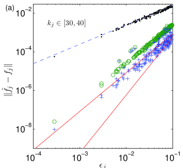
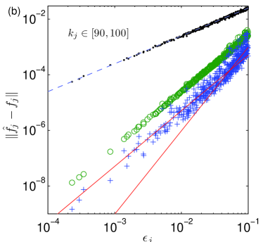
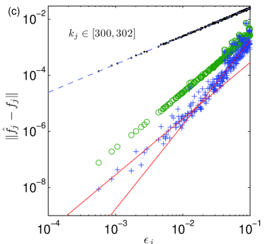
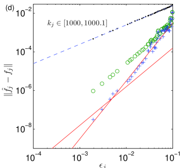
Figure 6. Boundary error norms of three eigenfunction prediction schemes for four different $k$ ranges, vs ${\epsilon}_{j}:=k_{j}-k_{*}$. Trivial scheme (dots), using (28), is compared against $0.25{\epsilon}$ (dotted line). Linearized scheme (circles), using (75) is shown. Quadratic scheme (crosses), using (77), is compared against power laws $0.5{\epsilon}^{2}k^{-1/2}$ and $0.1{\epsilon}^{3}k^{1/2}$. The domain is as in Fig. 1.

5.2. Higher-order reconstruction of eigenfunctions

In order to find higher order estimators for the Dirichlet eigenfunction (or more precisely, its normal derivative at the boundary), we first compute the $k$-derivative of an eigenfunction branch $f(k)$ of $\Theta(k)$. For simplicity we assume the eigenspace is simple.

Taking the derivative of (6) gives the formula

$$(\Theta-\beta)\dot{f}=(\dot{\beta}-\dot{\Theta})f.$$ (66)

Now fix $k_{0}\in[k_{*},k_{*}+\epsilon]$ and let $v(k)$ be as in (14), hence satisfying (15) and (16). Also, at $k=k_{0}$ we have

$$v(k_{0})|_{{\partial\Omega}}=\beta(k_{0})f(k_{0}).$$ (67)

We make the observation that, due to the commutation formula

$$\big{[}\Delta,x\cdot\nabla\big{]}=2\Delta,$$

the function $x\cdot\nabla v/k$ satisfies

$$(\Delta+k^{2})\Big{(}\frac{1}{k}x\cdot\nabla v\Big{)}=-2kv.$$

Therefore, combining this with (16), the function $q:=\dot{v}-\frac{1}{k}x\cdot\nabla v$ is Helmholtz for every $k$, and so we have, at $k=k_{0}$, a relation between the value and normal derivative of $q$ on the boundary,

$$(\Theta-\beta)(x\cdot n)q_{n}\;=\;q|_{\partial\Omega}-\beta(x\cdot n)q_{n}~{}.$$

Using the second part of (16) this simplifies to the following at $k=k_{0}$,

$$\frac{1}{k}\big{(}\Theta-\beta\big{)}(x\cdot n)\partial_{n}(x\cdot\nabla v)\;=\;-\dot{v}|_{\partial\Omega}+\frac{1}{k}(x\cdot\nabla v)|_{\partial\Omega}-\frac{\beta}{k}(x\cdot n)\partial_{n}(x\cdot\nabla v)~{}.$$ (68)

We need to re-express the spatial 2nd-derivatives in terms of the boundary ${\partial\Omega}$. The Laplace-Beltrami operator $\Delta_{\partial\Omega}$ is related to the Laplacian in ${\mathbb{R}}^{d}$ by

$$\Delta=\partial_{nn}+(d-1)H\partial_{n}+\Delta_{\partial\Omega}~{},$$ (69)

where the scalar function $H$ is the mean curvature of ${\partial\Omega}$. Thus, for any Helmholtz function $w$, writing the scalar function $h:=-(d-1)(x\cdot n)H$, we have,

$$((x\cdot n)\partial_{n})^{2}w\big{|}_{{\partial\Omega}}=-(x\cdot n)^{2}(\Delta_{{\partial\Omega}}+k^{2})w|_{\partial\Omega}+(1+h)(x\cdot n)w_{n}~{}.$$ (70)

Writing $x\cdot\nabla$ at the boundary as $(x\cdot n)\partial_{n}+W$, we also compute, for any smooth function $w$, that,

$$\big{[}(x\cdot n)\partial_{n},x\cdot\nabla\big{]}w\big{|}_{{\partial\Omega}}=g(x\cdot n)w_{n}+W^{\prime}w~{},$$ (71)

where $g:=-(x\cdot n)^{-1}W(x\cdot n)$ is a scalar function, and $W^{\prime}$ is a tangential derivative operator on ${\partial\Omega}$ whose vector field is given by the covariant derivative of $n$ with respect to the dilation vector field $x\cdot\nabla$. Here we extend the normal vector $n=(n_{1},\dots,n_{d})=\sum n_{i}e_{i}$ into a neighbourhood of ${\partial\Omega}$ so that it is of unit length and constant along lines perpendicular to the boundary. Explicitly,

$$W^{\prime}:=(x\cdot n)\sum_{i,j=1}^{d}x_{i}\frac{\partial n_{j}}{\partial x_{i}}\partial_{x_{j}}~{}.$$ (72)

One may check that $g+h+1=m$ from (61), via the identity $h=\operatorname{div}W-1$. Thus combining (70) and (71), and inserting (67) and $(x\cdot n){v}_{n}=f$, we get

$$(x\cdot n)\partial_{n}(x\cdot\nabla v)\;=\;(W+m)f-\beta(x\cdot n)^{2}(\Delta_{{\partial\Omega}}+k^{2})f+\beta W^{\prime}f~{}.$$

Acting on this with $\frac{1}{k}(\Theta-\beta)$ then equating with (68), replacing $\dot{v}$ via (15), and again expanding $x\cdot\nabla v$ gives, at $k=k_{0}$,

$$\frac{1}{k}\big{(}\Theta -\beta\big{)}\Big{(}(W+m)f+\beta W^{\prime}f-\beta(x\cdot n)^{2}(\Delta_{{\partial\Omega}}+k^{2})f\Big{)}$$

$$=-\dot{\Theta}f+\frac{1}{k}\Big{(}f+\beta Wf\Big{)}-\frac{\beta}{k}\Big{(}(W+m)f-\beta(x\cdot n)^{2}(\Delta_{{\partial\Omega}}+k^{2})f\Big{)}$$

$$=(\dot{\beta}-\dot{\Theta})f+\big{(}\frac{1}{k}-\dot{\beta})f-\frac{\beta}{k}\Big{(}mf+\beta W^{\prime}f-\beta(x\cdot n)^{2}(\Delta_{{\partial\Omega}}+k^{2})f\Big{)}.$$

Notice that the $\beta Wf/k$ terms canceled in the last step. Combined with (66), and observing that the range of $\Theta-\beta$ is orthogonal to $f$, we get

$$\frac{1}{k}\big{(}\Theta -\beta\big{)}\Big{(}(W+m)f+\beta W^{\prime}f-\beta(x\cdot n)^{2}(\Delta_{{\partial\Omega}}+k^{2})f\Big{)}$$

$$=(\Theta-\beta)\dot{f}-\frac{\beta}{k}\Big{(}mf+\beta W^{\prime}f-\beta(x\cdot n)^{2}(\Delta_{{\partial\Omega}}+k^{2})f\Big{)}^{\perp}$$

where ^⟂ indicates projection onto the space orthogonal to $f$. Now applying $(\Theta-\beta)^{-1}$ (again we consider the generalized inverse, equal to zero on the span of $f$ and inverting $\Theta-\beta$ on the orthogonal complement), we find

$$\dot{f}=\frac{1}{k}\Big{(}(W+m)f+\beta W^{\prime}f-\beta(x\cdot n)^{2}(\Delta_{{\partial\Omega}}+k^{2})f\Big{)}\\ +\frac{\beta}{k}(\Theta-\beta)^{-1}\Big{(}mf+\beta W^{\prime}f-\beta(x\cdot n)^{2}(\Delta_{{\partial\Omega}}+k^{2})f\Big{)}+cf,$$ (73)

where the constant $c$ is determined by the normalization, i.e. $\langle\dot{f},f\rangle=0$.

From this we can determine the first and second derivatives of $f_{p}(k)$, the eigenfunction on the branch corresponding to Dirichlet eigenfrequency $k_{p}$, when $k=k_{p}$, that is, when $\beta=0$:

Proposition 5.2.

Let $(f(k),\beta(k))$ be an eigenpair for $\Theta(k)$, and let $D$ be the differential operator

$$D:=W+m-\frac{1}{2}{\left\langle{mf,f}\right\rangle}~{}.$$

Then if $\beta(k)=0$, the first and second derivatives for the eigenfunction $f(k)$ are

$$\dot{f} =\frac{1}{k}Df~{};$$ (74)

$$\ddot{f} =\frac{1}{k^{2}}\Big{(}(D^{2}-D)f-(x\cdot n)^{2}(\Delta_{{\partial\Omega}}+k^{2})f+W^{\prime}f+\Theta(k)^{-1}(mf)\Big{)}$$

$$\phantom{aaaaa}-\frac{1}{k^{2}}{\left\langle{mf,Df}\right\rangle}f+c_{1}f~{},$$

where $c_{1}$ is some normalization constant.

Proof.

The first identity follows from (73) by setting $\beta=0$, and computing that at $\beta=0$, noting that $W+m$ is adjoint to $-W$ with respect to (4),

$$c=-\frac{1}{k}{\left\langle{(W+m)f,f}\right\rangle}=-\frac{1}{2k}{\left\langle{mf,f}\right\rangle}.$$

The second formula follows by taking the $k$-derivative of the right hand side of (73) and then setting $\beta$ to zero, using (19). ∎

This proposition suggests that the following two estimators for $f(k_{p})$ should be more accurate than the trivial estimator $\hat{f}=f_{p}(k_{*})$ considered in Section 3.2. First, using just the first derivative formula in (74), we consider, with $f=f_{p}(k_{*})$, the

$$\mbox{``linear $f$ estimator'':}\qquad\hat{f}_{p}:=f+\frac{\hat{{\epsilon}}_{p}}{k_{*}}Df~{},\quad\mbox{ where }\hat{{\epsilon}}_{p}:=\hat{k}_{p}-k_{*}~{},$$ (75)

$\hat{{\epsilon}}_{p}$ being the best available estimate for $k_{p}-k_{*}$, e.g. via (65). Numerically in $d=2$ we handle the term $Wf=(x\cdot t)\partial_{t}f$ using a $N\times N$ spectral differentiation matrix [55, Ch. 3] applied to the discretized $f$; the FFT could also be used. Referring to the data shown by circles in Fig. 6, for the domain of Fig. 1(b), we see that empirically, this estimator is second-order accurate in $\epsilon$, with a constant that is independent of $k$. This improves upon the trivial estimator by one to three extra digits of accuracy.

In principle, one should be able to use the second derivative of $f$ given by (74) to obtain a third order accurate estimator. Unfortunately, this formula involves the operator $\Theta(k_{p})^{-1}$ which is not known explicitly; it could be approximated numerically at a cost of $O(N^{3})$, but this would need to be done afresh at each eigenfrequency and thus destroy the $O(N^{2})$ complexity per mode. However, if we study the size of the terms in the second derivative formula (74), we see that some of them can be expected to be lower order (in $k$) than others. For example, the terms $k^{-2}Df$ and $W^{\prime}f$ are lower order than $k^{-2}D^{2}f$. Also, as discussed in Remark D.3, subject to a spectral nonconcentration assumption, $k^{-2}\Theta(k_{p})^{-1}(mf)$ is typically a factor $k^{1/2}$ smaller than the leading terms. The normalization constant $c_{1}$ is also irrelevant to the order of accuracy we seek (we will instead normalize numerically). Thus, keeping the leading terms in (74),

$$\ddot{f}\;\approx\;\frac{1}{k^{2}}\big{(}D^{2}-D-(x\cdot n)^{2}(\Delta_{{\partial\Omega}}+k_{*}^{2})\big{)}f~{}.$$ (76)

At this order we also need to consider linear variation in $\dot{f}$, so we approximate $\dot{f}(\hat{k}_{p})$ by substituting (75) into the $\dot{f}$ formula in (74), that is,

$$\hat{\dot{f}}_{p}\;=\;\frac{1}{k_{*}}D\Big{(}f+\frac{\hat{{\epsilon}}_{p}}{k_{*}}Df\Big{)}~{}.$$

A second-order $f$ expansion about $\hat{k}_{p}$ then gives $\hat{f}_{p}=f+\hat{{\epsilon}}_{p}\hat{\dot{f}}_{p}-(\hat{{\epsilon}}_{p}^{2}/2)\ddot{f}$, which we can simplify, noting the sign change in the $D^{2}$ term, to the improved

$$\mbox{``quadratic $f$ estimator'':}\quad\hat{f}_{p}:=f+\frac{\hat{{\epsilon}}_{p}}{k_{*}}Df+\frac{\hat{{\epsilon}}_{p}^{2}}{2k_{*}^{2}}\big{(}D^{2}+D+(x\cdot n)^{2}(\Delta_{{\partial\Omega}}+k_{*}^{2})\big{)}f~{}.$$ (77)

As before, we use the best available $\hat{{\epsilon}}_{p}$ estimate. In $d=2$ we approximate $\Delta_{\partial\Omega}f=\partial_{tt}f$ via a spectral differentiation matrix. Finally we normalize $\hat{f}_{p}$ numerically.

Figure 6 (data shown by crosses) shows the improved accuracy of this estimator: it gives typically one extra digit over (75), and up to four extra digits over the trivial estimator. This error data is also summarized in the last two columns of Table 1. The figures strongly suggest an empirical error of $O({\epsilon}^{2}k^{-1/2}+{\epsilon}^{3}k^{1/2})$ for this estimator. As expected from the above discussion, the first term is a factor $k^{1/2}$ smaller than the error of (75). As with the linear eigenfrequency estimator, the cubic term dominates for larger frequency distances ${\epsilon}\gg k^{-1}$, which are needed anyway in $d=2$ to capture more than $O(1)$ mode per frequency window. Thus, in the fast regime, this method has asymptotic eigenfunction error $O({\epsilon}^{3}k^{1/2})$. If it is desired to keep this error bounded as $k\to\infty$, one must choose ${\epsilon}<k^{-1/6}$ rather than the ${\epsilon}=O(1)$ allowed for bounded eigenfrequency error. This reduces the speed-up factor of the NtD method slightly from $O(N)$ to $O(N^{5/6})$ in $d=2$.

In section 6 we will give rigorous estimates on the Riccati estimator (65) and linear $f$ estimator (75), assuming that the spectrum of $\Theta(k_{*})$ does not concentrate near $\beta_{p}$.

a) b)

Figure 7. Eigenfunctions of the pentafoil domain. (a) mode from the two-dimensional eigenspace at $k_{j}=300.005956478458\cdots$ (function is not $D_{5}$-symmetric); note scarring on a periodic orbit. (b) simple (hence $D_{5}$-symmetric) mode at $k_{j}=300.03832269\cdots$. (All digits believed correct.) Density shows $|\hat{\phi}_{j}|^{2}$, with white being zero. Parameters are as in first row of Table 2.

Figure 8. An eigenfunction of the pentafoil domain in the two-dimensional eigenspace with $k_{j}=1000.00302930323\cdots$ (all digits believed correct). There are around 400 wavelengths across the domain. Parameters are as in second row of Table 2.

				time / mode (sec)			abs error of $\hat{k}_{j}$		$L^{2}$-error of $\hat{f}_{j}$
$k$ interval	$j$	$N$	$n_{m}$	ref	NtD	ratio	max	median	max	median
$[300,300.1]$	2.3e4	2700	20	6500	20	320	3e$-7$	2e$-7$	1.0e$-3$	1.3e$-4$
$[1000,1000.1]$	2.6e5	9000	51	–	250	1000∗	–	–	–	–

Table 2. Runtimes and errors for the pentafoil domain of Figs. 7 and 8. Details are as in Table 1, except that in the reference method the absolute $k_{j}$ errors were only around $10^{-7}$, so errors below this are not discernable. For degenerate pairs, subspace angle replaces $L^{2}$-error (see Remark 5.3). Dashes show experiments not performed, and asterisk ($\ast$) indicates estimated ratio.

5.3. Performance in a domain with abundant degeneracies

Having constructed higher-order estimators and tested them in a nonsymmetric domain, we now apply them to a “pentafoil” domain parametrized by $r(\theta)=1+0.3\cos(5\theta)$. For group-theoretic reasons (it has the dihedral symmetry group $D_{5}$), its Dirichlet eigenfrequencies are generically either simple or a doubly-degenerate pair. As before, we found that an $N$ of around $6.3$ points per wavelength on ${\partial\Omega}$ gave full double-precision accuracy in computing the spectrum of $\Theta(k_{*})$. Table 2 summarizes our experiments comparing the proposed NtD method (using the Riccati (65) and quadratic (77) estimators) against the reference solver of App. B. Observe that error levels of the NtD method are similar to those for the previous domain, thus degeneracies seem to have no deleterious effect on error.

Remark 5.3.

For simple eigenvalues, as before, the $L^{2}$ error $\|\hat{f}_{j}-f_{j}\|$ was measured, with $\|\hat{f}_{j}\|=\|f_{j}\|=1$. For $p$-fold degenerate eigenvalues we used its generalization, the principal angle between subspaces. Here, one subspace is the eigenspace computed by the NtD method, while the other is that computed by the reference method. In the small angle limit and $p=1$ this is equivalent to the $L^{2}$ error.

Note that the reference method was slower, by roughly a factor of three compared to the nonsymmetric domain of Fig. 1(b), due to the difficulty of resolving eigenfrequency pairs. (Here a large tolerance tol = 1e-6 was chosen to limit this slow-down.) In contrast, the NtD method pays no penalty for close or exact degeneracies—this is one of its main advantages—thus its speed-up factors are around three times better than for the former domain at similar frequencies.

In Figs. 7 and 8 we show some eigenfunctions coming from the calculations of the first and second rows of Table 2 respectively. In the latter case, forming and diagonalizing the matrix of size $N=9000$ took 3.6 hrs and returned 51 modes. Based on the previous domain, we expect mediam error similar to those in the first row of the table. However, since for the mode shown, $k_{j}$ is so close to $k_{*}$ that we expect $\hat{k}$ error to be limited by machine precision ($10^{-13}$ absolute error), and eigenfunction $L^{2}$ error to be $10^{-7}$. We did not attempt to run a reference calculation here (it would have taken 3 weeks), but using the $O(N^{3})$ scaling from our previous tests, we estimate that our method is faster than the reference method by a factor of $10^{3}$.

To create Fig. 8, evaluation of the representation (27) on a grid of $8.2\times 10^{5}$ points took only 27 sec per eigenfunction using the Helmholtz fast multipole method (FMM) implementation of Gimbutas–Greengard [27]. The entire eigenmode calculation and plot is done by the following MPSpack code:

s = segment.smoothstar(9000, 0.3, 5);
d = domain(s, 1); s.setbc(-1, ’D’); p = evp(d);
o.eps = 0.1; o.modes = 1; o.khat = ’r’; o.fhat = ’s’;
p.solvespectrum([1000 1000.1], ’ntd’, o);
o = []; o.inds = 1; o.dx = 0.002; o.fmm = 1; o.col = ’bw’; showmodes(p, o);

The third line selects the Riccati esimator for $\hat{k}$ and the quadratic estimator for $\hat{f}$.

Remark 5.4.

If a domain has a known symmetry (such as the $D_{5}$ symmetry of this pentafoil example), it is possible to reduce $N$ by desymmetrizing and finding eigenfunctions in each symmetry class separately [6, 8]. This is often done in high-frequency studies [9] because it increases efficiency by a significant factor. For simplicity, we did not implement that here.

6. Error analysis of higher-order methods

In this section we specialize to the case of two dimensions, $d=2$. This allows us to use the exploit the relatively large mean spacing of Dirichlet eigenfrequencies in two dimensions (relative to higher dimensions).

6.1. A spectral nonconcentration assumption

All error estimates in this section will be conditional on the following assumption:

Assumption 6.1 (Absence of Spectral Concentration at scale $\eta$).

Let $\eta$ be a positive real number, and let $\beta$ be a negative eigenvalue of $\Theta(k)$ satisfying

$$-\frac{\epsilon}{k}\leq\beta\leq 0.$$

We say that there is absence of spectral concentration at $\beta$ at the scale $\eta$ if $\beta$ is the only eigenvalue of $\Theta(k_{*})$ (counted with multiplicity) in the interval

$$\big{[}\beta-\frac{\eta}{k^{2}},\ \min(\beta+\frac{\eta}{k^{2}},0)\big{]}.$$

This implies, in particular, that $\beta$ is a simple eigenvalue.

Notice that the eigenfrequencies of $\Delta$ are spaced $\sim 1/k$ apart on average when $d=2$, so in view of (45), the eigenvalues of $\Theta(k_{*})$ are spaced $\sim 1/k^{2}$ apart on average. Therefore, for sufficiently small $\eta$, we can expect that typically Assumption 6.1 is satisfied for most eigenvalues $\beta$ of $\Theta(k_{*})$ in the range $[-\epsilon/k,0]$, uniformly in $k$. We will always assume that $\eta\leq 1$ in our estimates below.

One simple consequence of (52) is that, if $\epsilon$ is not too large relative to $\eta$, Assumption 6.1 implies that the eigenvalue branch $\beta_{p}(k)$ is well-separated from neighbouring branches on the whole interval $[k_{*},k_{p}]$, where $\beta(k_{p})=0$:

Lemma 6.2.

Assume that $d=2$ and that the eigenvalue $\beta_{p}$ of $\Theta(k_{*})$ lies in the interval $[-\epsilon/k,0]$ and satisfies Assumption 6.1 at scale $\eta$. If $\eta$ satisfies

$$\eta\geq 8C\epsilon^{2},\quad\eta\geq 8C\epsilon^{3}k,$$ (78)

then $\beta_{p}(k)$ satisfies Assumption 6.1 at the scale $\eta/2$ for all $k\in[k_{*},k_{p}]$. Here the constant $C$ is the implied constant in (52).

Proof.

Let $\beta_{p}(k)$ and $\beta_{q}(k)$ be two negative eigenvalue branches of $\Theta(k)$, with $\beta_{q}(k)>\beta_{p}(k)$. Then (disregarding the trivial case in which $\beta_{q}(k_{*})=0$) we have

$$|\beta_{p}(k_{*})-\beta_{q}(k_{*})|\geq\frac{\eta}{k^{2}}.$$

We will show that

$$|\beta_{p}(k)-\beta_{q}(k)|\geq\frac{\eta}{2k^{2}}$$

for all $k>k_{*}$ for which both eigenbranches are defined (i.e. such that both $\beta_{p}(k)\leq 0$ and $\beta_{q}(k)\leq 0$). Using (52) we have

$$\Big{|}\frac{d}{dk}\big{(}\beta_{p}(k)-\beta_{q}(k)\big{)}\Big{|}\leq 2C\big{(}\frac{\epsilon}{k^{2}}+\frac{\epsilon^{2}}{k}\big{)},$$

since $|\beta_{p}(k)|,|\beta_{q}(k)|\leq\epsilon/k$ for all $k\geq k_{*}$. Integrating over the interval $[k_{*},k]$ which is no bigger than $\epsilon$ for $k\leq k_{p}$, we find that

$$\begin{gathered}|\beta_{p}(k)-\beta_{q}(k)|\geq|\beta_{p}(k_{*})-\beta_{q}(k_{*})|-2C\big{(}\frac{\epsilon^{2}}{k^{2}}+\frac{\epsilon^{3}}{k}\big{)}\\ \geq\frac{\eta}{k^{2}}-2C\big{(}\frac{\epsilon^{2}}{k^{2}}+\frac{\epsilon^{3}}{k}\big{)}\\ \geq\frac{\eta}{2k^{2}},\end{gathered}$$

using the conditions (78) in the last step. ∎

6.2. Error estimate for second-order eigenfunction reconstruction

We now give an error estimate for the estimator (75), given Assumption 6.1 at scale $\eta$. We begin with

Lemma 6.3.

Assume $d=2$. For $k_{0}\in[k_{*},k_{*}+\epsilon]$ and $-\epsilon/k\leq\beta(k_{*})\leq 0$, the $k$-derivative of $f$ satisfies

$$\dot{f}=\frac{1}{k}(W+m)f+O(\frac{\epsilon+\epsilon^{2}k}{\eta})$$ (79)

where $W$ is as in (47) and $m$ as in (61).

Proof.

Consider the terms on the right hand side of (73). Indeed, using Lemma 4.4 (and Remark 4.5 for the higher order derivatives), and since $|\beta|\leq\epsilon/k$, we see that

$$\frac{\beta}{k}\|W^{\prime}f\|\leq\frac{\epsilon}{k},\quad\frac{\beta}{k}\|(x\cdot n)^{2}(\Delta_{{\partial\Omega}}+k^{2})f\|\leq\epsilon.$$

Next, using Proposition D.2 and Assumption 6.1 at scale $\eta$, we can estimate the remaining terms on the right hand side of (73) as follows:

$$\Big{\|}\frac{\beta}{k}(\Theta-\beta)^{-1}\Big{(}\beta(x\cdot n)^{2}(\Delta_{{\partial\Omega}}+k^{2})f-\beta W^{\prime}f-mf\Big{)}\Big{\|}$$

$$\leq C\frac{|\beta|}{k}\frac{k^{2}}{\eta}\big{\|}\beta(x\cdot n)^{2}(\Delta_{{\partial\Omega}}+k^{2})f-\beta W^{\prime}f-mf\big{\|}_{L^{2}({\partial\Omega})}$$

$$\phantom{33}+C\frac{|\beta|}{k}\big{\|}\beta(x\cdot n)^{2}(\Delta_{{\partial\Omega}}+k^{2})f-\beta W^{\prime}f-mf\big{\|}_{H^{1}({\partial\Omega})}$$

$$=\frac{C|\beta|k}{\eta}\big{(}|\beta|k^{2}+|\beta|k+1\big{)}+\frac{C|\beta|}{k}\big{(}|\beta|k^{3}+|\beta|k^{2}+k\big{)}$$

$$\leq\frac{C}{\eta}\big{(}\epsilon+\epsilon^{2}k\big{)}.$$

Here we used Lemma 4.4 and Remark 4.5 to estimate the $L^{2}$ and $H^{1}$ norms in the second and third lines. Finally, the term $cf$ is the result of projecting orthogonally onto the subspace orthogonal to $f$, so this term does not increase the norm. We conclude (79). ∎

This leads to

Proposition 6.4.

Suppose that $d=2$ and that $\beta(k_{*})=\beta_{p}(k_{*})$ satisfies Assumption 6.1 at scale $\eta$. Let $f_{p}=(x\cdot n)\partial_{n}\phi_{p}/\|(x\cdot n)\partial_{n}\phi_{p}\|$. Then the estimator (75) for $f(k_{p})$ satisfies

$$\|\hat{f}_{p}-f_{p}\|_{L^{2}({\partial\Omega})}=O(\frac{\epsilon^{2}+\epsilon^{3}k}{\eta}).$$ (80)

Proof.

To do this, we consider two flows. One is the eigenfunction flow (73) above. The second, for the function $g=g(k)$, is the linear flow starting at $g(k_{*})=f(k_{*})$, and flowing according to

$$\dot{g}=\frac{1}{k}(Wf(k_{*})+mf(k_{*})).$$

Note that the RHS here is independent of $k$ (apart from the $1/k$ prefactor). Now we estimate the difference between $g(\hat{k})=g(k_{*}/(1+\beta))$ and the weighted normal derivative of the corresponding Dirichlet eigenfunction. This is a sum of two terms: one arising from the difference between $g(\hat{k})$ and $f(\hat{k})$, and one arising from the difference between $f(\hat{k})$ and $f(k_{p})$, where $k_{p}$ is the true eigenvalue. Using (46) and Lemma 6.3, together with Lemma 4.4 to see that $\|Wf\|/k=O(1)$, the second error term is

$$O\big{(}\frac{\epsilon^{2}}{k}+\epsilon^{3}\big{)}\times O\big{(}1+\frac{\epsilon+\epsilon^{2}k}{\eta}\big{)}=O\big{(}\frac{\epsilon^{2}}{k}+\epsilon^{3}+\frac{\epsilon^{3}}{k\eta}+\frac{\epsilon^{4}}{\eta}+\frac{\epsilon^{5}k}{\eta}\big{)},$$

which is certainly bounded by (80) for large $k$ and $\eta\leq 1$.

The first difference can be estimated as follows. We have, with $f_{*}=f(k_{*})$,

$$\begin{gathered}\frac{d}{dk}{(f-g)}=\frac{1}{k}\Big{(}(W+m)(f-f_{*})\Big{)}+O(\frac{\epsilon+\epsilon^{2}k}{\eta})\\ =\frac{1}{k}\Big{(}(W+m)(f-g)\Big{)}+\frac{1}{k}\Big{(}(W+m)(g-f_{*})\Big{)}+O(\frac{\epsilon+\epsilon^{2}k}{\eta}).\end{gathered}$$

Since $g-f_{*}=O(\epsilon)$ (and using Lemma 4.4 again) the second term can be absorbed in the error term, and we get

$$\frac{d}{dk}{(f-g)}=\frac{1}{k}\Big{(}(W+m)(f-g)\Big{)}+O(\frac{\epsilon+\epsilon^{2}k}{\eta}).$$

Again applying Lemma 4.4, we have $k^{-1}\|(W+m)(f-g)\|\leq C\|f-g\|$. Therefore,

$$\frac{d}{dk}\Big{(}e^{-C(k-k_{p})}\|f-g\|_{L^{2}}\Big{)}=O(\frac{\epsilon+\epsilon^{2}k}{\eta})e^{-C(k-k_{p})}.$$

Since $(f-g)(k_{*})=0$, this inequality integrates to

$$\|(f-g)(k)\|_{L^{2}}=O(\frac{\epsilon^{2}+\epsilon^{3}k}{\eta})\text{ for }|k-k_{*}|\leq\epsilon.$$ (81)

In particular,

$$\|(f-g)(\hat{k}_{p})\|_{L^{2}}=O(\frac{\epsilon^{2}+\epsilon^{3}k}{\eta}).$$ (82)

∎

6.3. Error estimate for the Riccati eigenfrequency estimator

Here we derive an error estimate for the higher-order eigenfrequency estimator of section 5.1, given Assumption 6.1 at scale $\eta$.

Proposition 6.5.

Let the frozen frequency be $k_{z}=k_{*}$. Then the estimator (65) for the eigenfrequency $k_{p}$ satisfies

$$|k_{p}-\hat{k}_{p}|\leq C\big{(}\frac{\epsilon^{3}}{k^{2}}+\frac{\epsilon^{4}}{k\eta}+\frac{\epsilon^{5}}{\eta}+\frac{k\epsilon^{6}}{\eta}\big{)}.$$ (83)

Note that if we work in a regime with ${\epsilon}=O(1)$, then in the high frequency limit the term $O(k{\epsilon}^{6}/\eta)$ dominates in this estimate. However, as we showed in section 5.1, empirically the dominant error is only $O({\epsilon}^{5})$. When $k_{z}=\mbox{\small$\frac{1}{2}$}(1+(1+\beta_{*})^{-1})k_{*}$ is used instead of $k_{z}=k_{*}$, empirically the $O({\epsilon}^{4}/k)$ term is also absent, reducing errors slightly at intermediate ${\epsilon}$ values.

Proof.

Consider the error in estimating the right hand side of (62) by (64). We compute

$$\frac{d}{dk}\|(x\cdot n)f\|^{2}=2\langle\dot{f},(x\cdot n)^{2}f\rangle=\frac{2}{k}\langle(W+m)f,(x\cdot n)^{2}f\rangle+O(\frac{\epsilon+\epsilon^{2}k}{\eta}).$$ (84)

By integrating by parts, we see that

$$\frac{1}{k}\Big{|}{\left\langle{(W+m)f,(x\cdot n)^{2}f}\right\rangle}\Big{|}\leq\frac{C}{k}$$

(uniformly in $\epsilon$ and $k$). Therefore, for any $k_{0}\in[k_{*},k_{*}+\epsilon]$, the difference between the value of $k\beta^{2}\|(x\cdot n)f\|^{2}$ (i.e. the second term of (62)) at $k_{0}$ compared to the value at $k_{*}$ is bounded by

$$Ck\beta^{2}\cdot\epsilon\big{(}\frac{1}{k}+\frac{\epsilon+\epsilon^{2}k}{\eta}\big{)}=O\big{(}\frac{\epsilon^{3}}{k^{2}}+\frac{\epsilon^{4}}{k\eta}+\frac{\epsilon^{5}}{\eta}\big{)}.$$

A similar calculation shows that the difference between the third term of (62) at $k_{0}$ compared to the value at $k_{*}$ is again $O(\epsilon^{3}/k+\epsilon^{4}/(k\eta)+\epsilon^{5}/\eta)$. Treating the fourth and last term of (62) similarly, we obtain an error estimate of $O(\epsilon^{2}/k^{2}+\epsilon^{3}/(k^{2}\eta)+\epsilon^{4}/(k\eta))$ between the value of this term at $k_{0}$ compared to the value at $k_{*}$.

Therefore, the error term in $\beta$ for any $k_{0}\in[k_{*},k_{*}+\epsilon]$ is bounded by integrating this error on the interval $[k_{*},k_{*}+\epsilon]$ and is therefore bounded by $O(\epsilon^{3}/k^{3}+\epsilon^{4}/(k^{2}\eta)+\epsilon^{5}/(k\eta)+\epsilon^{6}/\eta)$. Finally, since the derivative $d\beta/dk$ is comparable to $1/k$ (say, between $1/2k$ and $2/k$) by (52), we see that the error in the estimate for $k_{p}$ is bounded by (83). ∎

7. Connection to the scaling method of Vergini–Saraceno

Our above proposed NtD method is closely related to, indeed inspired by, the scaling method of Vergini–Saraceno [61]. Here we explain briefly the latter, using the language of numerical mathematics (the original paper is very short and written in a physics style), thus improving upon previous understandings [8, 9]. We at least heuristically explain its observed accuracy, and highlight the many differences with the present NtD method.

7.1. Sketch of the scaling method

The method exploits the fact that a scaled, or dilated, Helmholtz solution is still Helmholtz. Let $\Phi(k)$, $k\neq k_{j}$, be the operator mapping Dirichlet data to the dilational derivative of its interior Helmholtz extension, that is, given $g\in H^{1}({\partial\Omega})$, and $u$ satisfying its Dirichlet problem (3), its action is

$$\Phi(k)g=x\cdot\nabla u|_{\partial\Omega}~{}.$$

Now consider a Dirichlet eigenfunction $\phi_{j}$, and let $f=(x\cdot n)\partial_{n}\phi_{j}|_{{\partial\Omega}}$. Take a frequency $k_{*}=k_{j}-\epsilon$ where $\epsilon>0$ is small, and define $\phi_{j}(k_{*})$ to be the dilation of the function $\phi_{j}$ to this new frequency $k_{*}$, that is

$$\phi_{j}(k_{*})(x):=\phi_{j}\bigl{(}\frac{k_{*}}{k_{j}}x\bigr{)}~{},\qquad x\in{\mathbb{R}}^{d}$$ (85)

Then to first order in $\epsilon$, we have

$$\phi_{j}(k_{*})|_{{\partial\Omega}}=-\frac{\epsilon}{k}(1+O(\epsilon))f$$ (86)

and

$$x\cdot\nabla\phi_{j}(k_{*})|_{{\partial\Omega}}=(1+O(\epsilon))f~{}.$$ (87)

The last two equations tell us that the dilated eigenmode $\phi_{j}(k_{*})|_{\partial\Omega}$, is an approximate eigenfunction of $\Phi(k_{*})$ with approximate eigenvalue $-k/\epsilon$.

The scaling method uses a linearized self-adjoint version of the above. Let $\Phi^{\ast}$ be the adjoint of $\Phi$ with respect to (4). The eigenvalue problem used is (analogous to (6)),

$$\frac{1}{k_{*}}(\Phi(k_{*})+\Phi^{\ast}(k_{*}))\,h=\mu h~{}.$$ (88)

Although not stated as such, this is solved with the Galerkin method [37, Sec. 13.5] using a set of (MPS) global basis functions $\xi_{i}(k):\overline{\Omega}\to\mathbb{C}$, $i=1,\ldots,N$, each satisfying $(\Delta+k^{2})\xi_{i}(k)=0$ in $\overline{\Omega}$. The original basis choice was plane waves (which seem to require $\Omega$ to be convex [8]); since then, fundamental solutions [9] and Fourier-Bessel wedge solutions [11] have also been used to handle nonconvex domains with one singular corner. The action of $\Phi$ on $\xi_{i}|_{\partial\Omega}$ is known analytically because each $\xi_{i}$ is an interior Helmholtz solution. Then the Galerkin approximation to (88) is the generalized eigenvalue problem

$${\mathbf{G}}h^{(N)}=\mu^{(N)}{\mathbf{F}}h^{(N)}~{},$$ (89)

where the ‘mass’ matrix ${\mathbf{F}}$ has elements ${\mathbf{F}}_{ij}=\langle\xi_{i},\xi_{j}\rangle$, and ${\mathbf{G}}$ has elements ${\mathbf{G}}_{ij}=(\langle\xi_{i},x\cdot\nabla\xi_{j}\rangle+\langle x\cdot\nabla\xi_{i},\xi_{j}\rangle)/k_{*}$. Further assuming that $\xi_{i}(k)(x)=\tilde{\xi}_{i}(kx)$, $x\in\overline{\Omega}$ i.e. the basis $k$-dependence is dilational, one may then check that ${\mathbf{G}}=d{\mathbf{F}}/dk|_{k=k_{*}}$, explaining Eq. (2) of [61]. In practice, it is well known that good global bases are highly ill-conditioned [16, 42], thus ${\mathbf{F}}$ and ${\mathbf{G}}$ share a numerical nullspace. Then (89) must be regularized, e.g. by projection onto the numerical range of one of the matrices, in a similar fashion to [15, 10].

Reconstruction of eigenfrequencies is via $\hat{k}=k_{*}-2/\mu$, and empirically has accuracy $O({\epsilon}^{3})$ [8], not the $O({\epsilon}^{4})$ claimed in [61]. Eigenmodes are reconstructed from the corresponding eigenvector components $h_{i}^{(N)}$ by “undoing” the dilation via $\hat{\phi}=\sum_{i=1}^{N}h^{(N)}_{i}\xi_{i}(\hat{k})$; boundary error $\|\hat{\phi}\|_{L^{2}({\partial\Omega})}$ is then dominated empirically by $O({\epsilon}^{3})$ with unknown $k$-dependence [8, sec. 6.3].

7.2. Connecting scaling and NtD methods via dilation

In place of (87) one could instead write

$$(x\cdot n)\partial_{n}\phi_{j}(k_{*})=(1+O(\epsilon))f~{},$$

which, with (86), tells us that $f$ is an approximate eigenfunction of $\Theta(k_{*})$ with eigenvalue $-\epsilon/k$. It is this that motivated the authors to consider the weighted NtD flow—arguably more closely related to spectral theory of the Laplacian on $\Omega$—as an alternative to dilation.

To connect the eigenfrequency estimators of the methods, we note that $\Phi(k)=\Theta(k)^{-1}+W$, where $W$ is the tangential vector field in (47), and hence that $\Phi(k)+\Phi(k)^{*}=2\Theta(k)^{-1}-m$, where $m$ is defined by (61). Thus the operator appearing in (88) can be written as $(2/k_{*})\Theta(k_{*})^{-1}$ plus $k_{*}^{-1}$ times a multiplication operator; this shows that the eigenvalues of (88) and $\Theta(k_{*})$ are related by $\mu=(2/k_{*})(\beta^{-1}+O(1))$ as $k_{*}\to k_{j}$. Thus one predicts that the scaling method has eigenfrequency accuracy no better than that of (20); this is observed numerically.

For eigenfunction error, the authors are not aware of an explanation of why in the scaling method the combination of (88) and reconstruction by dilation has error as high-order as $O({\epsilon}^{3})$, as opposed to the naive $O({\epsilon})$. Presumably the spectral flow of (88) is very close to the flow with $k$ of $\phi_{j}(k)|_{\partial\Omega}$ under exact dilation. However, we may also connect our quadratic NtD estimator (77) to this exact dilational flow. Let $u$ be a Helmholtz solution, and let $f:=(x\cdot n){u}_{n}$ and $g:=u|_{{\partial\Omega}}$ be Cauchy data for its dilation $u(k)$ to frequency $k$. Then one can check that $f$ and $g$ satisfy a second-order evolution equation on ${\partial\Omega}$ of the form

$$\frac{d}{dk}\,{\biggl{[}\begin{matrix}g\\ f\end{matrix}\biggr{]}}=L\biggl{[}\begin{matrix}g\\ f\end{matrix}\biggr{]}$$

where

$$L=\biggl{[}\begin{matrix}L_{11}&L_{12}\\ L_{21}&L_{22}\end{matrix}\biggr{]}=\frac{1}{k}\biggl{[}\begin{matrix}W&1\\ -(x\cdot n)^{2}(\Delta_{{\partial\Omega}}+k^{2})+W^{\prime}&W+m\end{matrix}\biggr{]}.$$

From this we can derive the first and second derivatives of $f$ when $g=0$:

$$\dot{f} =\frac{1}{k}(W+m)f;$$ (90)

$$\ddot{f} =\frac{1}{k^{2}}\Big{(}(W+m)^{2}f-(W+m)f-(x\cdot n)^{2}(\Delta_{{\partial\Omega}}+k^{2})f\Big{)}.$$

Comparing to (74), we can see that the first derivative for this dilation flow at $\beta=0$ agrees with the first derivative for the $\Theta(k)$ flow, up to an irrelevant normalization term. Moreover, the second derivative terms agree to highest order (if we agree that the $\Theta^{-1}(mf)$ term is lower order as per Remark D.3). Consequently (77) corresponds to the dilation flow just as well as it does for the $\Theta(k)$ flow.

7.3. Advantages of NtD method over the scaling method

Although the NtD and scaling methods have similar eigenfunction error, share the same $O(N)$ acceleration factor and both are restricted to star-shaped domains, the NtD method has several advantages:

• Higher-order accuracy in eigenfrequencies is possible (see section 5.1), giving 3 to 5 extra correct digits in practice (Fig. 5).

• Modes are reconstructed via (27), without recourse to dilation (the latter requires continuation of basis functions to a strip lying outside of $\Omega$).

• A formulation in terms of the NtD operator allows rigorous estimates such as Propositions 4.2, 80 and 83.

• The NtD method, as implemented in Sec. 3, is robust at all choices of $k_{*}$, whereas the scaling method is known to lose accuracy as $k_{*}$ approaches each Dirichlet eigenfrequency [61, 8].

• Regularization of the numerically-singular pencil (89) requires a choice of small parameter that is not fully understood [61, 8, 9, 11].

• Our method leverages known spectrally-accurate discretizations of boundary integral operators, whereas the Galerkin method (89) implicit in the scaling method is limited by the accuracy of an available global MPS Helmholtz basis. Success of the latter basis is ad hoc and quite particular to the shape of $\Omega$.

However, on the last point, we note that some global bases are much more efficient than BIE because they need only 2–3 degrees of freedom per wavelength on the boundary [61, 9], and can be faster to evaluate than Hankel kernels.

8. Conclusions

We have presented, analyzed, and tested a fast algorithm for computing high-frequency Dirichlet eigenvalues and eigenmodes of smooth star-shaped domains in ${\mathbb{R}}^{d}$. The acceleration is achieved by linearizing, over a frequency distance ${\epsilon}$, the flow of the spectrum of the weighted NtD map. The choice of weight function $(x\cdot n)^{-1}$ is crucial since it equalizes the gradients in this flow and prevents “avoided crossings”. ${\epsilon}$ controls both the total time to compute all modes lying in a given frequency interval, and their resulting errors. Windows of size ${\epsilon}$ are handled independently; the scheme is “embarrassingly parallel”. Maintaining bounded absolute eigenfrequency errors, one may choose ${\epsilon}=O(1)$, giving a speed-up of $O(k^{d-1})=O(N)$ over standard methods, and more robustness since no root-search is needed. This factor is in practice in $d=2$ roughly the number of wavelengths across the domain; we show an example where it is $10^{3}$.

We proved robustness (neither spurious nor missing modes, see Remark 4.7), a leading third-order absolute accuracy in eigenfrequencies, and, given a spectral nonconcentration assumption, third-order $L^{2}$-errors of mode boundary functions. This required developing some new results in the analysis of elliptic PDE of interest in their own right. Understanding the NtD spectral flow led to improved estimators that are empirically fifth-order for eigenfrequencies, and third-order for modes (with constant improved by factor $k^{1/2}$). Our scheme has many advantages over the scaling method (see section 7.3), including an integral operator formulation, rigorous error analysis, and much smaller eigenfrequency errors.

It is important to realize that the acceleration mechanism works at the operator level, and is therefore independent of any further acceleration that could be applied, such as: block iterative solvers to extract the small negative matrix eigenvalues (we used exclusively dense direct solvers in this work), and fast multipole or fast direct solvers to apply or compress the discretized operators. However, since we are in a high-frequency regime (oscillatory kernel), it is not at all obvious that fast solvers will make much difference; testing this is an obvious next step.

Other natural questions for future work include the following:

• Can the method be modified to remove the star-shaped restriction?

• Can a modified method (possibly using ideas from [13]) handle other homogeneous boundary conditions such as Neumann and Robin?

• What accuracy can be reached for domains with corners in $d=2$ or $d=3$ using appropriate BIE discretizations? (Note that the scaling method has been used with nonsmooth boundaries [61, 9, 11].)

• Can boundary error bounds on $\hat{f}$ be extended to $\hat{\phi}$? (see Remark 3.2).

• Can (77) be analyzed, or improved upon in practice, while preserving the $O(N)$ speed-up? One idea along these lines is high-order extrapolation from a ${\epsilon}$-grid of $k_{*}$ values; analysis would need the spectral flow for complex $k$.

The reader is encouraged to try out the algorithms presented here by downloading MPSpack from http://code.google.com/p/mpspack

Acknowledgments

This work has benefited from discussions with Timo Betcke, Doron Cohen, Lennie Friedlander, Rick Heller, and Eduardo Vergini. AB acknowledges the support of the National Science Foundation through grant DMS-0811005, and is grateful for Visiting Fellowships to the Mathematics Department, Australian National University in February 2007 and February 2009. AH acknowledges the support of the Australian Research Council through a Future Fellowship FT0990895 and Discovery Grant DP1095448 and thanks the Mathematics Department, Dartmouth College for its hospitality during a visit in July 2010.

Appendix A Smoothness of eigenvalues and eigenprojections in $k$

We are interested in the flow of eigenvalues and eigenprojections of the operator $\Theta$ in the parameter $k$. The operator $\Theta$ has a pole whenever $k^{2}$ is a Neumann eigenvalue of $\Omega$, and we wish to show that small negative eigenvalues and eigenprojections flow smoothly across such values of $k$. To do this we consider the Cayley transform of $\Theta$, as in (7). Recalling (35) in the case $\eta=1$, and solving for $f$ and $g$ in terms of $u_{n}$ and $u|_{{\partial\Omega}}$, we see that $R(k)f=g$ is equivalent to the existence of $u$ such that

$$\big{(}\Delta+k^{2})u=0,\quad f=iu|_{{\partial\Omega}}-(x\cdot n)\partial_{n}u|_{{\partial\Omega}},\quad g=iu|_{{\partial\Omega}}+(x\cdot n)\partial_{n}u|_{{\partial\Omega}}.$$ (91)

Proposition A.1.

There is a neighbourhood $U\subset{\mathbb{C}}$ of the positive real axis such that there is a unique solution to the problem

$$(\Delta+k^{2})u=0\text{ in }\Omega,\quad iu|_{{\partial\Omega}}-(x\cdot n)\partial_{n}u|_{{\partial\Omega}}=f$$ (92)

for every $k\in U$ and every $f\in L^{2}({\partial\Omega})$. Moreover, the solution $u=u(k)$ depends holomorphically on $k$ for $k\in U$.

Corollary A.2.

The Cayley transform $R(k)$ of $\Theta(k)$ is analytic in a neighbourhood $U\subset{\mathbb{C}}$ of the positive real axis.

Before we give the proof of this proposition we need a couple of preparatory lemmas.

Lemma A.3.

There is a neighbourhood $U\subset{\mathbb{C}}$ of the positive real axis such that for $k\in U$, the equation

$$(\Delta+k^{2})u=0\text{ in }\Omega,\quad iu|_{{\partial\Omega}}-(x\cdot n)\partial_{n}u|_{{\partial\Omega}}=0$$ (93)

has only the trivial solution.

Proof.

Write $k=a+ib$ with $a,b$ real. If $u$ satisfies (93), then we have

$$\begin{gathered}-k^{2}\int_{\Omega}|u|^{2}+\int_{\Omega}|\nabla u|^{2}=\int_{\Omega}(\Delta u)\,\overline{u}+\int_{\Omega}\nabla u\cdot\nabla\overline{u}\\ =\int_{{\partial\Omega}}\partial_{n}u\,\overline{u}=\int_{{\partial\Omega}}i(x\cdot n)^{-1}|u|^{2}.\end{gathered}$$ (94)

Taking the imaginary part we find that

$$-2ab\int_{\Omega}|u|^{2}=\int_{{\partial\Omega}}(x\cdot n)^{-1}|u|^{2}.$$ (95)

On the other hand, we can express $u$ in $\Omega$ via Green’s representation formula (25). It is standard that ${\mathcal{S}}(k)$ and ${\mathcal{D}}(k)$ are bounded operators from $L^{2}({\partial\Omega})$ to ${L^{2}(\Omega)}$, and it is straightforward to check that their norms are uniform in $k$ on compact subsets of the $k$-axis. Using the boundary condition for $u$ to replace $\partial_{n}u$ by $i(x\cdot n)^{-1}u$ in (25), we see that this gives

$$\|u(k)\|_{{L^{2}(\Omega)}}\leq C(k)\|u\|_{L^{2}({\partial\Omega})}$$

where $C(k)$ is uniform on compact subsets. But if we combine this with (95), then we see that for $|b|$ small enough compared to $a$, then (95) has only the trivial solution $u=0$. ∎

Lemma A.4.

There is a compact operator $L:L^{2}(\Omega)\to L^{2}(\Omega)$ such that $Lz$ is the unique solution $u$ to the equation

$$\Delta u=z\text{ in }\Omega,\quad iu|_{{\partial\Omega}}-(x\cdot n)\partial_{n}u|_{{\partial\Omega}}=0.$$

Proof.

We define operator $L_{1}$ to be inverse operator to the Dirichlet Laplacian on $\Omega$, i.e. $L_{1}z$ is the function $u_{1}$ such that $\Delta u_{1}=z$ in $\Omega$ with $u_{1}|_{{\partial\Omega}}=0$. It is standard that $L_{1}$ is well-defined and compact. We then try to solve

$$\Delta u_{2}=0\text{ in }\Omega,\quad iu_{2}|_{{\partial\Omega}}-(x\cdot n)\partial_{n}u_{2}|_{{\partial\Omega}}=(x\cdot n)\partial_{n}u_{1}|_{{\partial\Omega}};$$ (96)

then $u_{1}+u_{2}$ is the solution $u$ that we seek. Notice that (96) implies that

$$(x\cdot n)\partial_{n}u_{1}|_{{\partial\Omega}}=(i-B(0))u_{2}|_{{\partial\Omega}},$$

where $B(0)=(x\cdot n)\Lambda(0)$ is the weighted Dirichlet to Neumann operator at zero energy. The operator $B(0)$ is self-adjoint on $L^{2}({\partial\Omega})$ with our weighted inner product, so we can invert $i-B(0)$ and find that

$$u_{2}|_{{\partial\Omega}}=(i-B(0))^{-1}((x\cdot n)\partial_{n}u_{1}|_{{\partial\Omega}}).$$

Finally, if $P$ is the classical Poisson operator taking functions on ${\partial\Omega}$ to the harmonic function in $\Omega$ with the given boundary value, then we have

$$u_{2}=P\circ(i-B(0))^{-1}(x\cdot n)\partial_{n}L_{1}z.$$

We recall some standard mapping properties of these operators. The operator $L_{1}$ maps $L^{2}(\Omega)$ to $H^{2}(\Omega)$, then $(x\cdot n)$ times the normal derivative of this at the boundary maps to $H^{1/2}({\partial\Omega})$, then $(i-B(0))^{-1}$ is a pseudodifferential operator of order $-1$, hence maps $H^{1/2}(\Omega)$ to $H^{3/2}(\Omega)$, while $P$ maps $H^{3/2}(\Omega)$ to $H^{2}(\Omega)$ [53, Ch. 5, Prop. 1.7]. Denote the composite operator $L_{2}$, i.e. $u_{2}=L_{2}z$. Then we see that $L_{2}$ maps $L^{2}(\Omega)$ continuously to $H^{2}(\Omega)$, and hence, using the compact embedding of $H^{2}(\Omega)$ into $L^{2}(\Omega)$, we see that $L_{2}$ is compact on $L^{2}(\Omega)$. Hence $L=L_{1}+L_{2}$ is compact. Uniqueness of the solution follows from Lemma A.3 with $k=0$. This completes the proof of Lemma A.4. ∎

Proof of Proposition.

Let $U$ be as in Lemma A.3. Then this lemma guarantees the uniqueness of $u$ satisfying (92). It remains to establish existence. To do this, we first find $w_{1}$ such that

$$\Delta w_{1}=0\text{ in }\Omega,\quad iw|_{{\partial\Omega}}-(x\cdot n)d_{n}w_{1}|_{{\partial\Omega}}=f$$

which is done exactly as in (96). Then we look for $w_{2}$ satisfying

$$(\Delta+k^{2})w_{2}=-k^{2}w_{1},\quad iw_{2}-(x\cdot n)\partial_{n}w_{2}|_{{\partial\Omega}}=0.$$

If we can find such a $w_{2}$, then $u=w_{1}+w_{2}$ is our required solution of (92). Using the operator $L$ from Lemma A.4, this can be written

$$w_{2}=-L(k^{2}w_{1}+k^{2}w_{2}),$$

which is equivalent to

$$\big{(}\operatorname{Id}+k^{2}L\big{)}w_{2}=-k^{2}Lw_{1}.$$

Thus we get a solution provided that $\operatorname{Id}+k^{2}L$ is invertible. Since $L$ is compact, this will be the case provided that $\operatorname{Id}+k^{2}L$ has trivial null space. But if $v$ is in the null space of this operator then $v$ satisfies (93), which means by Lemma A.3 that indeed $v=0$. Therefore the null space is trivial, so $\operatorname{Id}+k^{2}L$ is invertible and we can find $w_{2}$ as above. This establishes existence of $u$. Finally, using the compactness of $L$ and analytic Fredhom theory [49, Thm. VI.14], for $k\in U$, $(\operatorname{Id}+k^{2}L)^{-1}(-k^{2}Lw_{1})$ is analytic in $k$, showing that $u(k)$ is analytic in $k$. ∎

It follows from the analyticity of $R(k)$ that in any interval $I$ of the unit circle in which the spectrum of $R(k)$ is discrete at $k=k_{0}$, the eigenvalues of $R(k)$ in $I$ are analytic as a function of $k$, and one can choose an orthonormal basis of the corresponding eigenspaces that varies analytically [34, Ch. VII, sec. 3]. This implies that the eigenspaces of $\Theta(k)$ vary analytically in any interval where the spectrum is discrete, with the exception of a finite number that have a pole at each Neumann eigenfrequency. Since $\Theta(k)$ is a pseudodifferential operator of order $-1$ and therefore compact, this means that the eigenspaces vary analytically except when the eigenvalue hits zero. In fact, we can say more. Before we state the next proposition, recall that the eigenvalues of $\Theta(k)$ are monotonic increasing in $k$ — see (17).

Proposition A.5.

(i) Suppose that $0$ is an eigenvalue of $\Theta(k_{*})$. Then there is an analytic eigenvalue branch $\beta(k)$ with $\beta\uparrow 0$ as $k\uparrow k_{*}$, and the multiplicity of the $0$ eigenspace is equal to the sums of the multiplicities of all such branches.

(ii) Conversely, suppose that $\beta(k)$ is an eigenvalue branch of $\Theta(k)$ tending to zero as $k\uparrow k_{*}$. Then $k_{*}$ is a Dirichlet eigenfrequency, the eigenprojection has a limit as $k\uparrow k_{*}$, and it is the projection onto a subspace of the space of weighted normal derivatives of Dirichlet eigenfunctions with eigenfrequency $k_{*}$. The eigenvalue $\beta(k)$ is $C^{1}$ as a function of $k$ up to and including $k=k_{*}$, and satisfies (19). Finally, if the eigenvalue $\beta(k)$ is simple up to and including $k=k_{*}$, then the eigenfunction $f(k)$ is $C^{2}$ up to an including $k=k_{*}$, and satisfies (74).

Proof.

(i) Suppose that $0$ is an eigenvalue of $\Theta(k_{*})$, with eigenspace $V$. Choose an interval $(a,b)$ containing $0$, with neither $a$ nor $b$ in the spectrum of $\Theta(k_{*})$, and such that there are no eigenvalues in the interval $(a,0)$, and let $\Pi_{a,b}(k)$ denote the projection onto the eigenspaces of $\Theta(k)$ with eigenvalues in the interval $(a,b)$. Define $\tilde{\Theta}(k)=\Pi_{a,b}(k)\Theta(k)$. Then for $k$ close to $k_{*}$, $\tilde{\Theta}(k)$ is an analytic family, again using [34, Ch. VII, sec. 3]. By the calculation in Lemma 2.2, $d\tilde{\Theta}(k)/dk$ is a positive operator. Since

$${\left\langle{\tilde{\Theta}(k_{*})f,f}\right\rangle}=0\text{ for all }f\in V,$$

we have

$${\left\langle{\tilde{\Theta}(k)f,f}\right\rangle}<0\text{ for all }f\in V,\ k<k_{*}.$$

So there are at least $(\dim V)$ negative eigenvalues of $\tilde{\Theta}(k)$, which tend to $0$ as $k\uparrow k_{*}$. These branches are analytic for $k<k_{*}$ since the negative spectrum of $\tilde{\Theta}(k)$ is discrete. The statement that there are exactly $(\dim V)$ negative eigenvalues of $\tilde{\Theta}(k)$ which tend to $0$ as $k\uparrow k_{*}$ follows from the proof of (ii) below.

(ii) For simplicity, we first prove (ii) assuming that $\beta(k)$ is simple. In that case, taking the eigenfunction $f(k)$ to be normalized in $L^{2}({\partial\Omega})$, we see from the identity (110) that the extended eigenfunction $u(k)$ is uniformly bounded in $H^{1}(\Omega)$ as $k\uparrow k_{*}$. Therefore, there is a sequence $k_{i}$ tending upward to $k_{*}$ such that $u(k_{i})$ has a weak limit $v$ in $H^{1}(\Omega)$, and therefore, a strong limit in $L^{2}$, along this sequence. It also follows from (17) and (52) that the $L^{2}$ norm of $u(k_{i})$ does not tend to zero along this sequence, so $v$ is nonzero. From the fact that the $u(k_{i})$ are Helmholtz, we find that along this sequence, we have

$$\lim\int_{\Omega}u(k_{i})(\Delta+k_{i}^{2})\psi=0\quad\text{for all }\psi\in C_{c}^{\infty}(\Omega),$$

implying that $v$ is a weak solution of the equation $(\Delta+k_{*}^{2})v=0$. By elliptic regularity, this means that $v$ is smooth in the interior of $\Omega$ and satisfies the equation in the strong sense. Also, using the continuous map from $H^{1}(\Omega)\to L^{2}({\partial\Omega})$ given by restriction to the boundary, we see that $v|_{{\partial\Omega}}$ is the weak limit (in $L^{2}({\partial\Omega})$) of $u(k_{i})|_{{\partial\Omega}}$. But $u(k_{i})|_{{\partial\Omega}}$ tends strongly to zero (since $u(k_{i})|_{{\partial\Omega}}=\beta(k_{i})f(k_{i})$ and $\beta(k_{i})$ tends to zero) and a fortiori weakly, so $v$ is zero at the boundary. It follows that $v$ is a Dirichlet eigenfunction. We see that $u(k)$ has a continuous extension to $k=k_{*}$, such that it is a Dirichlet eigenfunction at $k=k_{*}$. That is, $0$ is an eigenfunction of $\Theta(k_{*})$, so the eigenvalue branch $\beta(k)$ extends continuously to $k=k_{*}$. Given (54), we see that $\dot{\beta}$ has a limit $1/k_{*}$ as $k\uparrow k_{*}$, and therefore, $\beta(k)$ is $C^{1}$ up to an including $k=k_{*}$, and (19) holds.

If $\beta$ is a multiple eigenvalue, we proceed similarly. We take a sequence of extended eigenfunctions as before, and produce a Dirichlet eigenfunction $v_{1}$. Next we take another sequence of extended eigenfunctions orthogonal (at the same value of $k$) to the first sequence, and produce another Dirichlet eigenfunction $v_{2}$, and so on. We find a subspace of Dirichlet eigenfunctions at frequency $k_{*}$ of dimension equal to that of the multiplicity of $\beta(k)$.

Again assuming that the eigenvalue $\beta(k)$ is simple up to and including $k=k_{*}$, let $\eta$ be a positive number such that Assumption 6.1 holds in some interval $[k_{*}-\delta,k_{*}]$ for some $\delta>0$. Then Lemma 6.3 and Lemma 4.4, show that $\dot{f}(k)$ is uniformly bounded as $k\uparrow k_{*}$, and hence $f(k)$ has a limit as $k\to k_{*}$. Now referring to (73), using the continuity of $f(k)$ just shown, Lemma 4.4 and (51) to bound derivatives of $f(k)$, and Proposition D.2 to control the norm of $(\Theta(k)-\beta)^{-1}$ uniformly as $k\uparrow k_{*}$, we see that $\dot{f}$ itself is continuous up to $k=k_{*}$. Iterating once more using (73), we see that $\ddot{f}$ is continuous up to $k=k_{*}$. Hence $f(k)$ is $C^{2}$ up to $k=k_{*}$ and formula (73) extends by continuity to $k=k_{*}$ to yield (74) when $\beta=0$. ∎

Appendix B Computation of reference eigenfrequencies and eigenmodes

Here we describe our implementation of a standard published method for computation of eigenpairs, which we use as a reference to assess both accuracy and speed of the NtD method. Recalling the definition (30), we have the following standard result (e.g. see [41, Lemma 8.4] which applies for domains with Lipschitz boundary; note the opposite sign convention).

Lemma B.1.

A positive frequency $k$ is a Dirichlet eigenfrequency if and only if the operator $(\mbox{\small$\frac{1}{2}$}-D^{\ast}(k))$ has a non-trivial nullspace. Furthermore, its nullspace is precisely the space of boundary normal derivatives of solutions of $(\Delta+k^{2})u=0$ in $\Omega$ with homogeneous Dirichlet data on the boundary.

Its proof uses the jump relations and the uniqueness of the exterior Helmholtz Neumann boundary value problem [18, 41]. The numerical method is then, following Bäcker [6, sec. 3.3], to search along the $k$ axis for (near) zeros of the lowest singular value of a matrix discretization of the operator $(\mbox{\small$\frac{1}{2}$}-D^{\ast}(k))$. We use the Nyström quadrature as in (39)–(40); the same $N$ as before may be used to achieve quadrature errors around machine precision. The cost of each minimum singular value evaluation is then $O(N^{3})$. (We note that finding roots of the determinant is faster but is not able to distinguish close eigenfrequencies or handle degeneracies reliably [6]).

The minimum singular value, which we call $t$, as a function of $k$, has the form of a series of V-shapes with the bottom of each ‘V’ approaching zero (e.g. see Fig. 8 of [40] or Fig. 5.1 of [10]). Reliably locating all such minima in a range of $k$ is not trivial, crudely speaking because close eigenfrequencies lead to small-scale W-shapes that are difficult to distinguish from a ‘V’. We make use of the empirical observation that the slope of $t(k)$ appears to have an upper bound $C_{t}$ of size $O(1)$ which depends only on $\Omega$, and that most of the V-shapes have this slope. We initially evaluate $t(k)$ on a regular grid of spacing about 0.2 times the mean eigenfrequency spacing. At each local minimum on this grid we use the information about higher singular values to decide whether to i) perform fitting of a parabola to the three neighbouring samples of $t^{2}(k)$, and iterate this fit procedure until convergence, or ii) recursively call the same routine on an (about 3 times) finer grid covering three (or more, if there are nearby small values of $t$) neighbouring grid points. We omit several details of the algorithm required for robustness.

This has been coded into MPSpack and may be run (for instance for the example of section 3.1) via

o.maxslope = 1.5; o.tol = 1e-12; p.solvespectrum([90 100], ’ms’, o);

where maxslope defines the value $C_{t}$, and tol the requested absolute tolerance on $k$. When $C_{t}$ is chosen correctly, the algorithm finds all $k_{j}$ in a given $k$ interval, needing around 15 evaluations per simple eigenfrequency found, and typical errors are $10^{-13}$ or less. When eigenfrequencies are degenerate, many more recursions are needed to establish reliably that they are not distinct; for instance at o.tol = 1e-6 it still requires around 50 evaluations per multiple eigenfrequency found (this scales like log tol), and typical errors are $10^{-7}$.

Once accurate eigenfrequencies have been found, modes are found as follows. For each $k_{j}$, the last right singular vector of the above matrix is computed at a cost of $O(N^{3})$; according to Lemma B.1 this approximates $\partial_{n}\phi_{j}$ at the quadrature nodes. Normalization is done via (18). Eigenfunctions $\phi$ may then be reconstructed via (25). In the case of an $p$-fold degeneracy, the last $p$ right singular vectors are used. The whole method thus scales as $O(N^{3})$ per mode with a rather large constant.

Appendix C Proof of Lemma 4.4

Proof of Lemma 4.4.

We prove the theorem under very slightly more general conditions. That is, we replace $(x\cdot n)$ — both in the boundary condition (49) and in the weight factor in the inner product on $L^{2}({\partial\Omega})$ — by an arbitrary smooth positive weight, which we denote $m$. First, we introduce a spectral cutoff. Since we are using a weighted inner product we define the operator

$$\Delta_{\partial\Omega,w}=\nabla_{\tan}^{*,w}\nabla_{\tan}$$

on $L^{2}({\partial\Omega})$, where ^∗,w denotes the adjoint with respect to the weighted inner product. (Below, we write ^∗ instead of ^∗,w but all adjoints in this appendix should be understood to be with respect to the weighted inner product.) We write

$$\operatorname{Id}=\Psi(\Delta_{\partial\Omega,w}/k^{2})+(1-\Psi)(\Delta_{\partial\Omega,w}/k^{2}),\quad\text{ on }L^{2}({\partial\Omega}),$$

where $\Psi(t)$ is $1$ for $t\geq 3/2$ and $0$ for $t\leq 5/4$. Let us write $\Psi$ for $\Psi(\Delta_{\partial\Omega,w}/k^{2})$ below; note that $\Psi$ is a semiclassical pseudodifferential operator of order $(0,0)$, supported where $|\eta|\geq 3/2$. We can expect that the $L^{2}$ norm of $(\operatorname{Id}-\Psi)\nabla_{\tan}u$ is bounded by $2k$ times that of $u$, since applying $(\operatorname{Id}-\Psi)$ removes frequencies of order $\geq 2k$. To verify this, given a vector field $W$ of unit length and tangential to the boundary, we compute

$$\begin{gathered}\|(\operatorname{Id}-\Psi)Wu\|_{L^{2}({\partial\Omega})}^{2}=\|W(\operatorname{Id}-\Psi)u+[1-\Psi,W]u\|_{L^{2}({\partial\Omega})}^{2}\\ \leq\frac{4}{3}\|W(\operatorname{Id}-\Psi)u\|_{L^{2}({\partial\Omega})}^{2}+4\|[1-\Psi,W]u\|_{L^{2}({\partial\Omega})}^{2}\\ =\frac{4}{3}{\left\langle{(\operatorname{Id}-\Psi)W^{*}W(\operatorname{Id}-\Psi)u,u}\right\rangle}+4\|[1-\Psi,W]u\|_{L^{2}({\partial\Omega})}^{2}.\end{gathered}$$ (97)

Notice that $[1-\Psi,W]$ is a semiclassical pseudodifferential operator of order $(0,-\infty)$, hence with uniformly bounded (in $k$) $L^{2}({\partial\Omega})\to L^{2}({\partial\Omega})$ operator norm. If we sum over an orthonormal basis $W_{1},\dots,W_{n-1}$, then using $\sum_{i}W_{i}^{*}W_{i}=\Delta_{\partial\Omega,w}$ and the fact that $1-\Psi(t)$ vanishes when $t\geq 3/2$, we have

$$\begin{gathered}\|(\operatorname{Id}-\Psi)\nabla_{\tan}u\|_{L^{2}({\partial\Omega})}^{2}\leq 2{\left\langle{(\operatorname{Id}-\Psi)\Delta_{\partial\Omega,w}(\operatorname{Id}-\Psi)u,u}\right\rangle}+2\sum_{i}\|[1-\Psi,W_{i}]u\|_{L^{2}({\partial\Omega})}^{2}\\ \leq(2k^{2}+C)\|u\|_{L^{2}({\partial\Omega})}^{2}.\end{gathered}$$ (98)

Next we analyze the high energy part, $\Psi\nabla_{\tan}u$. We use the single and double layer boundary integral operators $S(k)$ defined by (29), and $D(k)$ defined by (30). We also write $Q(k)$ for the (hypersingular) operator $\partial_{n_{x}}\partial_{n_{y}}G_{0}(k;x,y)$ restricted to the boundary in both variables.

We now quote results from [29, Section 4]. Here it is shown that $S(k)$ and $D(k)$ are pseudodifferential operators of order $(-1,-1)$ in the ‘elliptic region’ $\{|\eta|>1\}$ (where $|\eta|$ is the length of $\eta$ with respect to the induced boundary metric on ${\partial\Omega}$), in the sense that if $\Phi$ is a semiclassical pseudodifferential operator of order $(l,m)$, microsupported in the elliptic region, then $\Phi S(k)$ and $\Phi D(k)$ are semiclassical pseudodifferential operators of orders $(l-1,m-1)$. Moreover, the analysis from [29, Section 4] applies to $\Phi Q(k)$ which shows that $\Phi Q(k)$ is a semiclassical pseudodifferential operator of order $(l+1,m+1)$, with principal symbol $-\mbox{\small$\frac{1}{2}$}k\sigma(\Phi)\sqrt{1-|\eta|^{2}}$ where $\sigma(\Phi)$ is the principal symbol of $\Phi$. (See Remark C.1 in case this is confusing.)

For any Helmholtz solution $u$ we have the Green’s representation formula (25). By differentiating normally at the boundary ${\partial\Omega}$, we obtain, using (33),

$$\partial_{n}u(x)=(D(k)^{t}+\mbox{\small$\frac{1}{2}$})\partial_{n}u-Q(k)u.$$ (99)

Let us write $\tilde{D}(k)$ for the kernel $m^{-1}D(k)m$. We then obtain from (99) and the boundary condition (49) that

$$\mbox{\small$\frac{1}{2}$}\beta m\partial_{n}u=\beta(\tilde{D}(k))^{t}(m\partial_{n}u)-\beta mQ(k)u\\ \implies u=2(\tilde{D}(k))^{t}u-2\beta mQ(k)u.$$ (100)

Next we differentiate tangentially, apply $\Psi$, and take the inner product with $\Psi Wu$, where $W$ is a tangential vector field of unit length. We obtain

$${\left\langle{\Psi Wu,\Psi Wu}\right\rangle}=2{\left\langle{\Psi^{2}W(\tilde{D}(k))^{t}u,Wu}\right\rangle}-2\beta{\left\langle{W^{*}\Psi^{2}WmQ(k)u,u}\right\rangle}.$$ (101)

Using the results of [29] mentioned above, we see that $\Psi^{2}W(\tilde{D}(k))^{t}$ is a semiclassical operator of order $(0,0)$, hence bounded on $L^{2}({\partial\Omega})$ uniformly in $k$. (Here we use the property of $\Psi$ that it is microsupported in the elliptic region, in fact in the region $\{|\eta|\geq 4/3\}$.) Hence the first term in (101) is estimated by

$$C\|u\|_{L^{2}({\partial\Omega})}\|\nabla_{\tan}u\|_{L^{2}({\partial\Omega})}.$$ (102)

In the second term, we have the operator $W^{*}\Psi^{2}WmQ(k)$. Since $W^{*}\Psi^{2}Wm$ is also a pseudodifferential operator microsupported in the elliptic region, and since $W$ and $W^{*}$ are of pseudodifferential operator $(1,1)$, we see that $W^{*}\Psi^{2}WmQ(k)$ is a pseudodifferential operator of order $(3,3)$, with principal symbol

$$-k^{3}|\sigma(hW)|^{2}m\psi^{2}(\eta)\sqrt{|\eta|^{2}-1}.$$ (103)

This is minus the square of a smooth symbol, namely

$$k^{3/2}m^{1/2}\psi(\eta)\sigma(ihW)(|\eta|^{2}-1)^{1/4}.$$

The sign of (103) is crucial, as it will effectively allow us to discard this term, which would otherwise be too big to estimate. This works as follows: by the pseudodifferential calculus, we have $W^{*}\Psi^{2}WmQ(k)=-B^{*}B+A_{2}$, with $A_{2},B$ semiclassical pseudos, $B$ of order $(3/2,3/2)$ and $A_{2}$ of order $(2,2)$. This term can therefore be expressed

$$2\beta\|Bu\|_{2}^{2}-2\beta{\left\langle{u,A_{2}u}\right\rangle}.$$

Since $A_{2}$ is supported in $\{|\eta|\geq 3/2\}$ we can write

$$A_{2}=\nabla_{\tan}^{*}A_{0}\nabla_{\tan}+A_{1}$$

with $A_{0}$ of order $(0,0)$ and $A_{1}$ of order $(1,1)$. Since $A_{1}$ can be chosen to be microsupported in the elliptic region, we have $A_{1}=A_{0}^{\prime}\cdot\nabla_{\tan}+A_{0}^{\prime\prime}$, where $A_{0}^{\prime}$ and $A_{0}^{\prime\prime}$ are pseudos of order $(0,0)$. Thus we have

$$-\beta{\left\langle{W^{*}\Psi^{2}WmQ(k)u,u}\right\rangle}=2\beta\|Bu\|_{2}^{2}-2\beta\Big{(}{\left\langle{\nabla_{\tan}u,A_{0}\nabla_{\tan}u}\right\rangle}+{\left\langle{A_{0}^{\prime}\Delta_{\partial\Omega,w}^{1/2}u+A_{0}^{\prime\prime}u,u}\right\rangle}\Big{)}.$$

This gives an estimate for the second term of (101) of the form

$$\beta\|Bu\|_{2}^{2}+C|\beta|\Big{(}\|\nabla_{\tan}u\|_{L^{2}({\partial\Omega})}^{2}+\|u\|_{L^{2}({\partial\Omega})}^{2}\Big{)}$$ (104)

(where we dropped the term $C|\beta|\|u\|_{L^{2}({\partial\Omega})}\|\nabla_{\tan}u\|_{L^{2}({\partial\Omega})}$ since it is controlled by the other terms on the right hand side). Combining (102) and (104), we find that

$$\begin{gathered}\|\Psi Wu\|_{2}^{2}\leq\beta\|Bu\|_{2}^{2}+C|\beta|\Big{(}\|\nabla_{\tan}u\|_{L^{2}({\partial\Omega})}^{2}+\|u\|_{L^{2}({\partial\Omega})}^{2}\Big{)}+C\|u\|_{L^{2}({\partial\Omega})}\|\nabla_{\tan}u\|_{L^{2}({\partial\Omega})}\\ \leq C|\beta|\Big{(}\|\nabla_{\tan}u\|_{L^{2}({\partial\Omega})}^{2}+\|u\|_{L^{2}({\partial\Omega})}^{2}\Big{)}+C\|u\|_{L^{2}({\partial\Omega})}\|\nabla_{\tan}u\|_{L^{2}({\partial\Omega})}\end{gathered}$$

where we are able to discard the $Bu$ term since $\beta<0$. Combining this with (98) and using the inequality $\|a+b\|^{2}\leq 3\|a\|^{2}/2+3\|b\|^{2}$ we find that

$$\|Wu\|_{2}^{2}\leq(3k^{2}+C)\|u\|_{L^{2}({\partial\Omega})}^{2}+C\|u\|_{L^{2}({\partial\Omega})}\|\nabla_{\tan}u\|_{L^{2}({\partial\Omega})}+C|\beta|\|\nabla_{\tan}u\|_{L^{2}({\partial\Omega})}^{2},$$

and summing over an orthonormal basis of $W$ we find that

$$\|\nabla_{\tan}u\|_{2}^{2}\leq(3k^{2}+C)\|u\|_{L^{2}({\partial\Omega})}^{2}+C\|u\|_{L^{2}({\partial\Omega})}\|\nabla_{\tan}u\|_{L^{2}({\partial\Omega})}+C|\beta|\|\nabla_{\tan}u\|_{L^{2}({\partial\Omega})}^{2}.$$

Finally we write

$$C\|u\|_{L^{2}({\partial\Omega})}\|\nabla_{\tan}u\|_{L^{2}({\partial\Omega})}\leq 4C^{2}\|u\|_{L^{2}({\partial\Omega})}^{2}+\frac{1}{16}\|\nabla_{\tan}u\|_{L^{2}({\partial\Omega})}^{2},$$

and observe that for $|\beta|\leq C/16$ we can absorb the $\|\nabla_{\tan}u\|_{2}^{2}$ terms on the left hand side to deduce

$$\|\nabla_{\tan}u\|_{2}^{2}\leq\frac{8}{7}(3k^{2}+4C^{2})\|u\|_{L^{2}({\partial\Omega})}^{2}.$$

For $k\geq K$, we have $8(3k^{2}+4C^{2})/7\leq 4k^{2}$ and we arrive at (50). ∎

Remark C.1.

Since $D(k)$ involves one extra derivative than $S(k)$, it might seem peculiar that $S(k)$ and $D(k)$ are both order $(-1,-1)$ in the elliptic region. In fact, the distributional limit of $\partial_{n_{y}}G_{0}(k;x,y)$ to the boundary in both variables is a pseudodifferential operator of order $(0,0)$ in the elliptic region, but the leading part of this operator is half the identity — supported at the diagonal — so it does not appear when the kernel function is restricted to the boundary in both variables; rather this part of the operator shows up as the $\frac{1}{2}$ in the jump formula (31). This does not happen for $Q(k)$, hence its order is two more than that of $S(k)$, as expected.

Appendix D Estimates involving $(\Theta-\beta)^{-1}$

To prepare for this operator norm estimate we first generalize an estimate from [12] from the Dirichlet boundary condition to the ‘near Dirichlet’ Robin boundary conditions, that is the boundary condition

$$u|_{{\partial\Omega}}-\beta(x\cdot n)\partial_{n}u|_{{\partial\Omega}}=0,\quad-\frac{\delta}{k}\leq\beta\leq 0,$$ (105)

where $\delta$ is small and $\beta<0$. This is a self-adjoint boundary condition and there is a corresponding orthonormal basis of eigenfunctions $\phi_{j}^{\beta}$, with eigenvalues $E_{j}^{\beta}=(k_{j}^{\beta})^{2}$. Then we have

Proposition D.1.

Let ${\partial\Omega}$ be smooth. Then there exists $\delta>0$ and a constant $C_{\Omega}$ depending only on $\Omega$ and $\delta$ such that the operator norm

$$\Big{\|}\sum_{|k-k_{j}^{\beta}|\leq 1}(x\cdot n)\partial_{n}\phi^{\beta}_{j}\langle(x\cdot n)\partial_{n}\phi^{\beta}_{j},\cdot\rangle\Big{\|}_{L^{2}({\partial\Omega}),(x\cdot n)^{-1}d\sigma}$$ (106)

is bounded by $C_{\Omega}k^{2}$, uniformly for $\beta$ in the range $[-\delta/k,0]$.

Proof.

We use the same method of proof as in [12], but with additional work since we no longer have our functions vanishing at the boundary.

Our starting point is the identity

$$\begin{gathered}\int_{\Omega}\phi[\Delta+k^{2},V]\phi=\int_{\Omega}(\Delta+k^{2})\phi V\phi\\ -\int\phi V(\Delta+k^{2})\phi+\int_{{\partial\Omega}}\phi\partial_{n}V\phi-\partial_{n}\phi V\phi.\end{gathered}$$ (107)

If we choose $V$ to be a smooth vector field equal to $(x\cdot n)\partial_{n}$ at the boundary, then the last term in (107) is $\|(x\cdot n)\partial_{n}\phi\|^{2}$. We can therefore express

$$\begin{gathered}\|(x\cdot n)\partial_{n}\phi\|^{2}=\int_{{\partial\Omega}}(x\cdot n)|\partial_{n}\phi|^{2}\\ =\int_{{\partial\Omega}}\phi\partial_{n}(x\cdot n)\partial_{n}\phi+\int_{\Omega}(\Delta+k^{2})\phi V\phi-\int_{\Omega}\phi[\Delta+k^{2},V]\phi-\int\phi V(\Delta+k^{2})\phi\\ =I+II-III-IV.\end{gathered}$$ (108)

The first step in the proof of Proposition D.1 is to estimate this squared $L^{2}$ norm when $\phi$ is an approximate eigenfunction, that is, a function satisfying

$$\|\phi\|_{L^{2}(\Omega)}=1,\quad\phi+\beta(x\cdot n)\partial_{n}\phi=0\text{ at }{\partial\Omega},\quad\big{\|}(\Delta+k^{2})\phi\big{\|}_{L^{2}(\Omega)}=O(k).$$ (109)

We claim that this implies that

$$\|(x\cdot n)\partial_{n}\phi\|_{L^{2}({\partial\Omega})}\leq Ck,$$

which we prove by estimating terms $I$ — $IV$ in (108) by by a constant times $k^{2}$. Before doing so, observe that using (105) and Lemma 4.4 any boundary term of the form

$$\int_{{\partial\Omega}}a_{1}k^{2}|\phi|^{2}+a_{2}|\nabla_{\tan}\phi|^{2}+ka_{3}\phi|\nabla_{\tan}\phi|+ka_{4}\phi\partial_{n}\phi+a_{5}\partial_{n}\phi|\nabla_{\tan}\phi|$$

where $a_{i}$ are bounded functions on ${\partial\Omega}$, not depending on $\phi$ or $k$, can be estimated by $C\delta\|\partial_{n}\phi\|_{2}^{2}$ and therefore (for sufficiently small $\delta$) can be absorbed in the left hand side; we will call them ‘acceptable’ boundary terms.

Consider the identity

$$\int_{\Omega}|\nabla\phi|^{2}=\int_{\Omega}(-\Delta\phi)\overline{\phi}+\int_{{\partial\Omega}}\partial_{n}\phi\overline{\phi}~{}.$$ (110)

For $\beta\leq 0$, the last term is negative using the boundary condition (105), implying (using (109)) that

$$\|\nabla\phi\|_{L^{2}(\Omega)}=O(k)\implies\|V\phi\|_{L^{2}({\partial\Omega})}=O(k).$$ (111)

Using this we see that the term $II$ on the right hand side of (108) is $O(k^{2})$.

Term $IV$ can be expressed after integration by parts as

$$\int_{\Omega}V\phi(\Delta+k^{2})\phi+(\operatorname{div}V\phi)(\Delta+k^{2})\phi-\int_{{\partial\Omega}}(x\cdot n)(V\cdot n)\phi(\Delta+k^{2})\phi.$$

The first two terms are dealt with as above. In the third term, we expand $\Delta=\partial_{n}^{2}+\Delta_{\partial\Omega}+(d-1)H\partial_{n}$. Notice that the $\partial_{n}^{2}$ term cancels term $I$ in (108) up to an acceptable boundary term. So we have to estimate the terms

$$\int_{{\partial\Omega}}\phi(\Delta_{\partial\Omega}+(d-1)H\partial_{n}+k^{2})\phi.$$

The $H\partial_{n}$ and $k^{2}$ terms are acceptable. The $\Delta_{\partial\Omega}$ term is estimated by integrating by parts to convert the integrand to $|\nabla_{\tan}\phi|^{2}$ which is also acceptable.

To estimate term $III$ we use the fact that $[\Delta,V]$ is a second order operator and therefore of the form of a finite sum $\sum V_{i}W_{i}$ where $V_{i}$, $W_{i}$ are smooth vector fields. We can integrate by parts modulo an acceptable boundary term and obtain

$$\int_{{\partial\Omega}}\sum V_{i}\phi W_{i}\phi,$$

and the $L^{2}$ norm is bounded by $C\|\nabla u\|_{L^{2}(\Omega)}^{2}=O(k^{2})$. This completes the proof that $\|(x\cdot n)\partial_{n}\phi\|_{L^{2}({\partial\Omega})}^{2}=O(k^{2})$.

The second step of the proof is the same as in [12]. For the reader’s convenience we repeat the argument here. We define an operator $T$ from the range of the spectral projector $1_{[k-1,k+1]}(\sqrt{-\Delta})$, that is, the vector space spanned by eigenfunctions of $-\Delta$ with eigenvalues in the range $[(k-1)^{2},(k+1)^{2}]$, to $L^{2}({\partial\Omega})$, by

$$T\phi=(x\cdot n)\partial_{n}\phi|_{{\partial\Omega}}.$$

Then, any such $\phi$ satisfies

$$\big{\|}(\Delta+k^{2})\phi\big{\|}_{L^{2}(\Omega)}\leq(2k+1)\big{\|}\phi\big{\|}_{L^{2}(\Omega)},$$

meaning that $\phi$ is (after normalization) an approximate eigenfunction in the sense of (109). So in the first step of the proof above, we showed that $\|T\phi\|\leq Ck\|\phi\|$, or in other words that $T$ has operator norm at most $Ck$. But the operator norm of $T$ is equal to that of $T^{*}$, and the operator that appears in (106) is precisely $TT^{*}$. Since the operator norm of $TT^{*}$ is precisely the square of the operator norm of $T$, this completes the proof of the theorem. ∎

We now prove an estimate on the term involving the generalized inverse $(\Theta-\beta)^{-1}$ in (73).

Proposition D.2.

Let $\beta$, for $k\in[k_{*},k_{*}+\epsilon]$, be an eigenvalue of $\Theta(k)$ satisfying $-\epsilon/k\leq\beta<0$ and satisfying Assumption 6.1 at the scale $\eta$. Assume also that $\eta$ satisfies (78). Then there exists $C$ depending only on $\Omega$ such that for any $z\in H^{1}({\partial\Omega})$, we have the estimate

$$\big{\|}(\Theta(k)-\beta)^{-1}z\big{\|}_{L^{2}({\partial\Omega})}\leq C\Big{(}\frac{k^{2}}{\eta}\|z\|_{L^{2}({\partial\Omega})}+\|z\|_{H^{1}({\partial\Omega})}\Big{)}.$$ (112)

Proof.

Let $f$ be the eigenfunction of $\Theta(k)$ with eigenvalue $\beta$. Let $\tilde{z}\in L^{2}({\partial\Omega})$ be the projection of $z$ into the subspace orthogonal to $f$. Let $v$ be a Helmholtz solution at frequency $k$ such that $(v-\beta(x\cdot n)\partial_{n}v)|_{{\partial\Omega}}=\tilde{z}$; then $(\Theta(k)-\beta)^{-1}z=\Pi^{\perp}_{f}(x\cdot n)\partial_{n}v|_{{\partial\Omega}}$, where $\Pi^{\perp}_{f}$ is the orthogonal projection onto the subspace orthogonal to $f$. We need to estimate the norm of $(x\cdot n)\partial_{n}v|_{{\partial\Omega}}$ relative to the norm of $z$; for this it suffices to assume $\tilde{z}=z$.

To estimate the size of $(x\cdot n)\partial_{n}v|_{{\partial\Omega}}$, we expand $v$ in eigenfunctions $\phi_{j}^{\beta}$ as in Proposition D.1. We write $E^{\beta}=k^{2}$. By assumption, there is a $j=j_{*}$ such that $E_{j_{*}}^{\beta}=E^{\beta}$; the corresponding eigenfunction $\phi_{j_{*}}^{\beta}$ satisfies $(x\cdot n)\partial_{n}\phi_{j_{*}}^{\beta}=f$.

Let

$$v=\sum a_{j}\phi^{\beta}_{j}.$$

We may assume that $a_{j_{*}}=0$, as $\Pi^{\perp}_{f}((x\cdot n)\partial_{n}\phi_{j_{*}}^{\beta})=0$. Then

$$\begin{gathered}a_{j}={\left\langle{v,\phi^{\beta}_{j}}\right\rangle}_{L^{2}(\Omega)}=\frac{1}{E^{\beta}-E^{\beta}_{j}}\Big{(}-{\left\langle{\Delta v,\phi^{\beta}_{j}}\right\rangle}+{\left\langle{v,\Delta\phi^{\beta}_{j}}\right\rangle}\Big{)}\\ =\frac{1}{E^{\beta}-E^{\beta}_{j}}\int_{{\partial\Omega}}v\partial_{n}\phi^{\beta}_{j}-\partial_{n}v\phi^{\beta}_{j}\\ =\frac{1}{E^{\beta}-E^{\beta}_{j}}\int_{{\partial\Omega}}v\partial_{n}\phi^{\beta}_{j}-\partial_{n}v\beta(x\cdot n)\partial_{n}\phi^{\beta}_{j}\\ =\frac{1}{E^{\beta}-E^{\beta}_{j}}\int_{{\partial\Omega}}z\partial_{n}\phi^{\beta}_{j}.\end{gathered}$$

Therefore,

$$v=\sum_{j\neq j_{*}}\Big{(}\frac{1}{E^{\beta}-E^{\beta}_{j}}\int_{{\partial\Omega}}z\partial_{n}\phi^{\beta}_{j}\Big{)}\phi^{\beta}_{j}.$$

If we try to take the normal derivative term by term in this series and sum, unfortunately we end up with a divergent series (even when the quasi-orthogonality of the boundary values $(x\cdot n)\partial_{n}\phi_{j}^{\beta}$ is taken into account). To avoid this problem we write $v^{\prime}$ as the solution to

$$\Delta v^{\prime}=0\text{ in }\Omega,\quad(v-\beta(x\cdot n)\partial_{n}v)|_{{\partial\Omega}}=z;$$

there is a unique solution to this problem due to the negativity of $\beta$. Then we can express $v^{\prime}=\sum a^{\prime}_{j}\phi^{\beta}_{j}$, where from a similar computation to above

$$a^{\prime}_{j}=-\frac{1}{E^{\beta}_{j}}\int_{{\partial\Omega}}z\partial_{n}\phi^{\beta}_{j}\quad(\implies a^{\prime}_{j_{*}}=0.)$$

Therefore, $v-v^{\prime}$ has an expansion

$$\begin{gathered}v-v^{\prime}=\sum_{j\neq j_{*}}\Big{(}\Big{(}\frac{1}{E^{\beta}-E^{\beta}_{j}}+\frac{1}{E_{j}^{\beta}}\Big{)}\int_{{\partial\Omega}}z\partial_{n}\phi^{\beta}_{j}\Big{)}\phi^{\beta}_{j}\\ =\sum_{j\neq j_{*}}\Big{(}\frac{E^{\beta}}{E^{\beta}_{j}(E^{\beta}-E^{\beta}_{j})}\int_{{\partial\Omega}}z\partial_{n}\phi^{\beta}_{j}\Big{)}\phi^{\beta}_{j}.\end{gathered}$$ (113)

which has improved convergence properties as the denominator is now $\sim(E_{j}^{\beta})^{-2}$ instead of $(E_{j}^{\beta})^{-1}$, as $j\to\infty$. From this we see that

$$(x\cdot n)\partial_{n}(v-v^{\prime})=\sum_{j\neq j_{*}}\Big{(}\frac{E^{\beta}}{E^{\beta}_{j}(E^{\beta}-E^{\beta}_{j})}\int_{{\partial\Omega}}z\partial_{n}\phi^{\beta}_{j}\Big{)}(x\cdot n)\partial_{n}\phi^{\beta}_{j}.$$

Now we use Proposition D.1, proceed as in Section 4 of [12] and show that the operator

$$z\mapsto\sum_{j\neq j_{*}}\Big{(}\frac{E^{\beta}}{E^{\beta}_{j}(E^{\beta}-E^{\beta}_{j})}\int_{{\partial\Omega}}z\partial_{n}\phi^{\beta}_{j}\Big{)}(x\cdot n)\partial_{n}\phi^{\beta}_{j}$$

has operator norm at most $C+Ck^{2}/d(E^{\beta},\sigma^{*})$, where $d(E^{\beta},\sigma^{*})$ denotes the distance from $E^{\beta}$ to the nearest point of the spectrum on $\Delta$ with boundary condition (105). By Assumption 6.1 and Lemma 6.2, this distance is at least $C\eta$, so we get an estimate on the operator norm of $Ck^{2}/\eta$. Therefore $v-v^{\prime}$ has norm at most $Ck^{2}/\eta\|z\|_{L^{2}({\partial\Omega})}$.

To treat the term $v^{\prime}$, notice that that $(x\cdot n)\partial_{n}v^{\prime}$ is $(\Theta(0)-\beta)^{-1}z$; we will estimate the operator norm of $(\Theta(0)-\beta)^{-1}$. The operator $\Theta(0)$ is a positive operator, since

$${\left\langle{v,(x\cdot n)\partial_{n}v}\right\rangle}=\int_{{\partial\Omega}}v\partial_{n}v=\int_{\Omega}v\Delta v+|\nabla v|^{2}\geq 0.$$

Therefore, as $\beta$ is negative, the norm of $(\Theta(0)-\beta)^{-1}z$ is no bigger than that of $\Theta(0)^{-1}z$. The operator $\Theta(0)^{-1}$, which is nothing other than the multiplication opertor $(x\cdot n)$ composed with the Dirichlet-to-Neumann map at energy zero, is a pseudodifferential operator of order $1$, and therefore

$$\|v^{\prime}\|_{L^{2}({\partial\Omega})}\leq C\|z\|_{H^{1}({\partial\Omega})}.$$

This concludes the proof of Proposition D.2. ∎

Remark D.3.

In fact, although the above analysis shows that $\|(\Theta(k)-\beta)^{-1}z\|$ can indeed be as large as $Ck^{2}/d(E^{\beta},\sigma^{*})$ times $\|z\|$, this only happens in a ‘worst-case scenario’ in which $z$ is a multiple of $\partial_{n}\phi_{j}^{\beta}$ where $E_{j}^{\beta}$ is the eigenvalue of $\Theta(k)$ closest to (but distinct from) $E^{\beta}$ (or, more precisely, a linear combination of an $O(1)$ number of the $(x\cdot n)\partial_{n}\phi_{j}^{\beta}$ with closest eigenvalues). In a more ‘typical-case scenario’, the coefficients $a_{j}$, for $|E_{j}^{\beta}-E^{\beta}|\leq\sqrt{E^{\beta}}$, would be $\sim k^{1/2}$ in magnitude — this can be seen from Proposition D.1 and the arguments of [12], which show that the $(x\cdot n)\partial_{n}\phi_{j}^{\beta}$ have norm $\sim k$ and are approximately orthogonal for $|E_{j}^{\beta}-E^{\beta}|\leq\sqrt{E^{\beta}}$. On the other hand, for $|E_{j}^{\beta}-E^{\beta}|\geq\sqrt{E^{\beta}}$, we gain a power of $\sqrt{E^{\beta}}=k$ in the denominator of (113). This suggests that, typically, we would have $\|(\Theta(k)-\beta)^{-1}z\|$ no bigger than a constant times $k^{3/2}\|z\|/d(E^{\beta},\sigma^{*})$. This would imply that in formula (74) for the second derivative of $f$ at $\beta=0$, and given Assumption 6.1 with $\eta\sim 1$, the $\Theta(k)^{-1}(mf)$ term is usually smaller by a factor $\sim k^{-1/2}$ than the principal terms, even though it is of the same order in the worst-case scenario. This is a heuristic justification for dropping this term in the quadratic estimator (77).

References

- [1] P. M. Anselone. Collectively compact operator approximation theory. Prentice-Hall, Englewood Cliffs, NJ, 1971.
- [2] K. Atkinson. The numerical solution of the eigenvalue problem for compact integral operators. Trans. Amer. Math. Soc., 129:458–465, 1967.
- [3] K. Atkinson. Convergence rates for approximate eigenvalues of compact integral operators. SIAM J. Numer. Anal., 12:213–222, 1975.
- [4] I. M. Babuska and J. Osborn. Eigenvalue problems. In P. G. Ciarlet and J. I. Lions, editors, Handbook of numerical analysis, Volume II, pages 643–787. Elsevier (North-Holland), 1991.
- [5] I. M. Babuska and S. A. Sauter. Is the pollution effect of the FEM avoidable for the Helmholtz equation considering high wave numbers? SIAM J. Numer. Anal., 34(6):2392–2423, 1997.
- [6] A. Bäcker. Numerical aspects of eigenvalue and eigenfunction computations for chaotic quantum systems. In The mathematical aspects of quantum maps, volume 618 of Lecture Notes in Phys., pages 91–144. Springer, Berlin, 2003.
- [7] A. Bäcker, R. Schubert, and P. Stifter. Rate of quantum ergodicity in Euclidean billiards. Phys. Rev. E (3), 57(5, part A):5425–5447, 1998. also see Errata for this paper, Phys. Rev. E, 58 (4) (1998).
-
[8]
A. H. Barnett.
Dissipation in deforming chaotic billiards.
PhD thesis, Harvard University, 2000.
available at
http://www.math.dartmouth.edu/~ahb/thesis_html/. - [9] A. H. Barnett. Asymptotic rate of quantum ergodicity in chaotic Euclidean billiards. Comm. Pure Appl. Math., 59(10):1457–88, 2006.
- [10] A. H. Barnett. Perturbative analysis of the Method of Particular Solutions for improved inclusion of high-lying Dirichlet eigenvalues. SIAM J. Numer. Anal., 47(3):1952–1970, 2009.
- [11] A. H. Barnett and T. Betcke. Quantum mushroom billiards. CHAOS, 17:043125, 2007.
- [12] A. H. Barnett and A. Hassell. Boundary quasi-orthogonality and sharp inclusion bounds for large Dirichlet eigenvalues. SIAM J. Numer. Anal., 49:1046–1063, 2011.
- [13] A. H. Barnett and A. Hassell. Estimates on Neumann eigenfunctions at the boundary, and the “Method of Particular Solutions” for computing them. In Spectral Geometry, proceedings of the International Conference on Spectral Geometry, Dartmouth College, 2011. submitted.
- [14] T. Betcke. A GSVD formulation of a domain decomposition method for planar eigenvalue problems. IMA J. Numer. Anal., 27:451–478, 2007.
- [15] T. Betcke and L. N. Trefethen. Reviving the method of particular solutions. SIAM Rev., 47(3):469–491, 2005.
- [16] O. Cessenat and B. Despres. Application of an ultra weak variational formulation of elliptic PDEs to the two-dimensional Helmholtz problem. SIAM J. Numer. Anal., 35(1):255–299, 1998.
- [17] D. Cohen, N. Lepore, and E. J. Heller. Consolidating boundary methods for finding the eigenstates of billiards. J. Phys. A, 37:2139–2161, 2004.
- [18] D. Colton and R. Kress. Integral equation methods in scattering theory. Wiley, 1983.
- [19] D. Colton and R. Kress. Inverse acoustic and electromagnetic scattering theory, volume 93 of Applied Mathematical Sciences. Springer-Verlag, Berlin, second edition, 1998.
- [20] R. Courant and D. Hilbert. Methods of mathematical physics. Vol. I. Interscience Publishers, Inc., New York, N.Y., 1953.
- [21] D. D. de Menezes, M. Jar E. Silva, and F. M. de Aguiar. Numerical experiments on quantum chaotic billiards. CHAOS, 17:023116, 2007.
- [22] B. Dietz, A. Heine, V. Heuveline, and A. Richter. Test of a numerical approach to the quantization of billiards. Phys. Rev. E, 71:026703, 2005.
- [23] T. A. Driscoll. Eigenmodes of isospectral drums. SIAM Rev., 39(1):1–17, 1997.
- [24] M. Durán, J.-C. Nédélec, and S. Ossandón. An efficient Galerkin BEM to compute high acoustic eigenfrequencies. J. Vib. Acoust., 131(3):03100(1–9), 2009.
- [25] L. Friedlander. Some inequalities between Dirichlet and Neumann eigenvalues. Arch. Rational Mech. Anal., 116(2):153–160, 1991.
- [26] P. R. Garabedian. Partial differential equations. John Wiley & Sons Inc., New York, 1964.
- [27] Z. Gimbutas and L. Greengard. HFMM2D, Fortran code for fast multipole method with Helmholtz kernel in two dimensions (version 20110313), 2011.
- [28] O. Giraud and K. Thas. Hearing shapes of drums: Mathematical and physical aspects of isospectrality. Rev. Mod. Phys., 82:2213–2255, 2010.
- [29] A. Hassell and S. Zelditch. Quantum ergodicity of boundary values of eigenfunctions. Comm. Math. Phys., 248(1):119–168, 2004.
- [30] E. J. Heller. Bound-state eigenfunctions of classically chaotic Hamiltonian systems: scars of periodic orbits. Phys. Rev. Lett., 53(16):1515–1518, 1984.
- [31] J. Helsing and R. Ojala. On the evaluation of layer potentials close to their sources. J. Comput. Phys., 227:2899–2921, 2008.
- [32] V. Heuveline. On the computation of a very large number of eigenvalues for selfadjoint elliptic operators by means of multigrid methods. J. Comput. Phys., 184:321–337, 2003.
- [33] A. Karageorghis. The method of fundamental solutions for the calculation of the eigenvalues of the Helmholtz equation. Appl. Math. Lett., 14(7):837–842, 2001.
- [34] T. Kato. Perturbation Theory for Linear Operators. Springer-Verlag, New York, 2nd edition, 1976.
- [35] S. M. Kirkup and S. Amini. Solution of the Helmholtz eigenvalue problem via the boundary element method. Int. J. Numer. Meth. Eng., 36(2):321–330, 1993.
- [36] R. Kress. Boundary integral equations in time-harmonic acoustic scattering. Mathl. Comput. Modelling, 15:229–243, 1991.
- [37] R. Kress. Linear Integral Equations, volume 82 of Applied Mathematical Sciences. Springer, second edition, 1999.
- [38] G. A. Kriegsmann. Scattering by large resonant cavity structures. Wave Motion, 30:329–344, 1999.
- [39] J. R. Kuttler and V. G. Sigillito. Eigenvalues of the Laplacian in two dimensions. SIAM Rev., 26(2):163–193, 1984.
- [40] P. G. Martinsson and V. Rokhlin. A fast direct solver for boundary integral equations in two dimensions. J. Comput. Phys., 205:1–23, 2005.
- [41] M. Mitrea. Boundary value problems and Hardy spaces associated to the Helmholtz equation in Lipschitz domains. J. Math. Anal. Appl., 202:819–842, 1996.
- [42] P. Monk and D.-Q. Wang. A least-squares method for the Helmholtz equation. Comput. Meth. Appl. Mech. Engrg., 175:121–136, 1999.
- [43] A. Nachman, J. Sylvester, and G. Uhlmann. An -dimensional Borg-Levinson theorem. Comm. Math. Phys., 115(4):595–605, 1988.
- [44] K. Nakamura and T. Harayama. Quantum Chaos and Quantum Dots. Oxford Univ. Press, 2004.
- [45] S. Nonnenmacher. Anatomy of quantum chaotic eigenstates. Séminaire Poincaré, XIV:177–220, 2010.
- [46] F. W. J. Olver, D. W. Lozier, R. F. Boisvert, and C. W. Clark, editors. NIST Handbook of Mathematical Functions. Cambridge University Press, 2010.
- [47] J. Osborn. Spectral approximation for compact operators. Math. Comput., 29:712–725, 1975.
- [48] T. Prosen. Quantization of a generic chaotic D billiard with smooth boundary. I. Energy level statistics. Phys. Lett. A, 233(4-6):323–331, 1997.
- [49] M. Reed and B. Simon. Methods of modern mathematical physics. I. Functional analysis. Academic Press Inc. [Harcourt Brace Jovanovich Publishers], New York, second edition, 1980.
- [50] F. Rellich. Darstellung der Eigenwerte von durch ein Randintegral. Math. Z., 46:635–636, 1940.
- [51] N. Saito. Data analysis and representation on a general domain using eigenfunctions of Laplacian. Applied and Computational Harmonic Analysis, 25:68–97, 2008.
- [52] O. Steinbach and G. Unger. A boundary element method for the Dirichlet eigenvalue problem of the Laplace operator. Numer. Math., 113:281–298, 2009.
- [53] M. E. Taylor. Partial Differential Equations: Basic Theory. Springer, Berlin, 1996.
- [54] The MathWorks, Inc. MATLAB software, Copyright (c) 1984–2011. http://www.mathworks.com/matlab.
- [55] L. N. Trefethen. Spectral methods in MATLAB, volume 10 of Software, Environments, and Tools. Society for Industrial and Applied Mathematics (SIAM), Philadelphia, PA, 2000.
- [56] L. N. Trefethen and T. Betcke. Computed eigenmodes of planar regions, volume 412 of Contemp. Math., pages 297–314. Amer. Math. Soc., Providence, RI, 2006.
- [57] H. E. Tureci and H. G. L. Schwefel. An efficient Fredholm method for calculation of highly excited states of billiards. J. Phys. A, 40:13869, 2007.
- [58] H. E. Tureci, H. G. L. Schwefel, P. Jacquod, and A. D. Stone. Modes of wave-chaotic dielectric resonators. Progress in Optics, 47:75–137, 2005.
- [59] G. Veble, T. Prosen, and M. Robnik. Expanded boundary integral method and chaotic time-reversal doublets in quantum billiards. New J. Phys., 9:15, 2007.
- [60] G. Veble, M. Robnik, and J. Liu. Study of regular and irregular states in generic systems. J. Phys. A, 32(36):6423–6444, 1999.
- [61] E. Vergini and M. Saraceno. Calculation by scaling of highly excited states of billiards. Phys. Rev. E, 52(3):2204–2207, 1995.
- [62] S. Zelditch. Quantum ergodicity and mixing of eigenfunctions. In Elsevier Encyclopedia of Mathematical Physics, volume 1, pages 183–196. Academic Press, 2006. arXiv:math-ph/0503026.