The holographic induced gravity model with a Ricci dark energy: smoothing the little rip and big rip through Gauss-Bonnet effects?

Abstract

We present an holographic brane-world model of the Dvali-Gabadadze-Porrati (DGP) scenario with and without a Gauss-Bonnet term (GB) in the bulk. We show that an holographic dark energy component with the Ricci scale as the infra-red cutoff can describe the late-time acceleration of the universe. In addition, we show that the dimensionless holographic parameter is very important in characterising the DGP branches, and in determining the behaviour of the Ricci dark energy as well as the asymptotic behaviour of the brane. On the one hand, in the DGP scenario the Ricci dark energy will exhibit a phantom-like behaviour with no big rip if the holographic parameter is strictly larger than 1/2. For smaller values, the brane hits a big rip or a little rip. On the other hand, we have shown that the introduction of the GB term avoids the big rip and little rip singularities on both branches but cannot avoid the appearance of a big freeze singularity for some values of the holographic parameter on the normal branch, however, these values are very unlikely because they lead to a very negative equation of state at the present and therefore we can speak in practice of singularity avoidance. At this regard, the equation of state parameter of the Ricci dark energy plays a crucial role, even more important than the GB parameter, in rejecting the parameter space where future singularities appear.

I Introduction

Various astrophysical observations of type Ia supernovae Perlmutter:1998np , cosmic microwave background (CMB) Komatsu:2010fb and large scale structure (LSS) Tegmark2004 , etc., suggest that the universe is in accelerating expansion. Quantitative analysis shows that there is a dark energy (DE) with negative pressure component leading to the dynamical mechanism of the accelerating expansion of the universe. However, the nature of this dark energy remains a mystery. Various models of dark energy have been proposed to solve this problem, such as a small positive cosmological constant Peebles and several kinds of scalar fields such as quintessence Ratra , k-essence ARMENDARIZ-PICON 2001 , phantom Caldwell , etc.

On the other hand, an alternative approach to explain the problem of DE arises from the holographic principle which states that the number of degrees of freedom for a system within a finite region should be finite and bounded by the area of its boundary 'tHooft:1993gx ; Susskind:1994vu . Furthermore it was also suggested that the ultraviolet (UV) cutoff scale of a system is connected to its infrared (IR) cutoff scale. Cohen et al. Cohen:1998zx pointed out that, for a system with size L and UV cutoff, which is not a black hole, the quantum vacuum energy of the system should not exceed the mass of the same size black hole, i.e. $L^{3}\rho_{\Lambda}\leq LM_{P}^{2}$, where $\rho_{\Lambda}$ is the vacuum energy density caused by UV cutoff $\Lambda$, and $M_{p}$ denotes the Plank mass ($M_{p}^{2}=1/8\pi G).$ The largest IR cutoff $L$ is required to saturate this inequality Li:2004rb ; Hsu:2004ri  and its holographic energy density is given by $\rho_{H}=3c^{2}M_{P}^{2}/L^{2}$, where $c$ is a phenomenological numerical constant. Later on, we will instead use the parameter $\beta$ defined as $\beta=c^{2}$. The holographic dark energy model is based on assuming that the energy density $\rho_{H}$ is responsible for the current speed up of the universe with $L$ being an appropriate cosmological length. It is well known that the length that plays the role of the IR cutoff on an holographic energy density is not unique. One of the choices of the IR cutoff is the Hubble rate. This choice does not induce acceleration either in a homogeneous and isotropic universe Hsu:2004ri or in the DGP model Wu:2007tp , but it does in the DGP model with a Gauss-Bonnet (GB) term in the bulk preparation (see also Ref. saridakis ). In the reference Li:2004rb , Li suggested that by choosing $L$ as the event horizon, the late-time acceleration of the universe is suitably described. Another choice for the IR cutoff $L$ was suggested by Gao et al. Gao (see also Nojiri:2005pu ), in which the IR cutoff of the holographic Ricci dark energy (RDE) was taken to be the Ricci scalar curvature.

Another approach to explain the observed acceleration of the late universe is to modify gravity at large scales. Models which describe this approach can be inspired by the existence of extra dimensions. The simplest and best studied case is the Dvali-Gabadadze-Porrati (DGP) model Dvali:2000hr . Such a model contains two kinds of solutions Deffayet:2000uy : the self-accelerating branch, which suffers from some problems, and the normal branch. Even though the normal branch is healthy it cannot describe the current acceleration of the universe unless a dark energy component is invoked BouhmadiLopez:2007ts or the gravitational action is modified BouhmadiLopez:2010pp . Modifying gravity at large scales by introducing a DGP brane-world model and taking into account curvature effects, as the GB term, were analysed in Kofinas:2003rz , richard , BouhmadiLopez:2008nf and preparation where it was shown that they can be quite useful to describe the current acceleration of the universe. The main aim of this paper is to show if the holographic RDE is suitable to describe the late time acceleration of the universe, avoiding at the same time a big rip or little rip in a DGP model with a Gauss-Bonnet term in the bulk.

The outline of the paper is as follows. In Sect. II we will review briefly the holographic DGP brane-world model with the Ricci scalar as an IR cutoff. In Sect. III, we analyse the modified Friedmann equation of the model without the Gauss-Bonnet term and we find analytically the asymptotical behaviour of the brane and numerically the whole expansion of the brane. In particular, we discuss the behaviour of the equation of state associated with the holographic Ricci dark energy and we show that for $\beta\leq 1/2$, $\beta$ being the holographic parameter, the solutions lead to a big rip or little rip. This motivate us to consider a GB term in the bulk action in order to enlarge the $\beta$ spectrum and overcome this problem. In Sect. IV, we consider the model where the bulk contains a GB term. We show that the effect of a GB term is to remove the little rip and big rip singularities on both branches, but it cannot avoid the appearance of a big freeze singularity for some values of the holographic parameter $\beta$ on the normal branch, however, these values are very unlikely because they lead to a very negative equation of state at the present and therefore we can speak in practice of singularity avoidance. At this regard, the equation of state parameter of the Ricci dark energy plays a crucial role, even more important than the GB parameter, in rejecting the parameter space where future singularities appear. Finally, in Sect. V, we conclude.

II Setup of the model

We consider a DGP brane-world model, where the bulk action contains a GB curvature term. The bulk corresponds to two symmetric pieces of a 5-dimensional (5d) Minkowski space-time. The brane is spatially flat and its action contains an induced gravity term. We assume that the brane is filled with matter and an holographic dark energy. Then, the modified Friedmann equation reads Kofinas:2003rz ; richard :

$$H^{2}=\frac{1}{3M_{P}^{2}}\rho+\frac{\epsilon}{r_{c}}\left(1+\frac{8\alpha}{3}H^{2}\right)H,$$ (1)

where $H$ is the brane Hubble parameter, $\rho=\rho_{\mathrm{m}}+\rho_{\mathrm{H}}$ is the total cosmic fluid energy density of the brane which can be described through a cold dark matter component (CDM) with energy density $\rho_{\mathrm{m}}$ and an holographic Ricci dark energy component with energy density $\rho_{\mathrm{H}}$. The parameters $r_{c}$ and $\alpha$ correspond to the cross over scale and the GB parameter, respectively, both of them being positive. The parameter $\epsilon$ in Eq. (1) can take two values: $\epsilon=1$, corresponding to the self-accelerating branch in the absence of any kind of dark energy richard ; and $\epsilon=-1$, corresponding to the normal branch which requires a dark energy component to accelerate at late-time preparation ; BouhmadiLopez:2010pp ; BouhmadiLopez:2008nf . For simplicity, we will keep the terminology: (i) self-accelerating branch when $\epsilon=1$ and (ii) normal branch when $\epsilon=-1$.

As already mentioned in the introduction, $\rho_{\mathrm{H}}$ is related to the UV cutoff, while $L$ is related to the IR cutoff. We consider a Ricci dark energy (RDE) Gao where the scale $L$ is fixed by $\mathcal{R}/6$, $\mathcal{R}$ being the scalar curvature of the brane. For a spatially flat Friedmann-Lemaître-Robertson-Walker (FLRW) universe

$$\mathcal{R=}6\left(\dot{H}+2H^{2}\right),$$

where the dot stands for the derivative with respect to the cosmic time of the brane. Therefore, the RDE energy density is

$$\rho_{\mathrm{H}}=3\beta M_{P}^{2}\left(\frac{1}{2}\frac{dH^{2}}{dx}+2H^{2}\right),$$ (2)

where $x=-\ln(z+1)=\ln(a)$, $z$ is the redshift and $\beta=c^{2}$ is a dimensionless parameter that measures the strength of the holographic component. As we will show, $\beta$ and Eq. (1) play a crucial role in determining the expansion of the RDE component. Before moving forwards, we would like to highlight that we have assumed that the holographic dark energy stated in Eq. (2) remains valid on brane-world models like the one we are considering here. A similar approach was followed in Refs. Wu:2007tp ; preparation .

The modified Friedmann equation (1) can be further rewritten as:

$$E^{2}=\Omega_{m}e^{-3x}+\beta(\dfrac{1}{2}\dfrac{dE^{2}}{dx}+2E^{2})+2\epsilon\sqrt{\Omega_{rc}}(1+\Omega_{\alpha}E^{2})E,$$ (3)

where $E(z)=H/H_{0}$ and

$$\Omega_{m} = \frac{\rho_{m_{0}}}{3M_{P}^{2}H_{0}^{2}},\,\,\,\,\Omega_{r_{c}}=\frac{1}{4r_{c}^{2}H_{0}^{2}},\text{\thinspace and }\,\Omega_{\alpha}=\frac{8}{3}\alpha H_{0}^{2}\,$$

are the usual convenient dimensionless parameters and the subscripts $0$ denotes the present value (we will follow the same notation as in BouhmadiLopez:2008nf ; preparation ). The dimensionless parameter of the holographic energy density can be written as:

$$\Omega_{\mathrm{H}}=\beta(\dfrac{1}{2}\dfrac{dE^{2}}{dx}+2E^{2}).$$ (5)

From (3) the variation of the dimensionless Hubble rate $E$ with respect to $x$ is

$$\dfrac{dE}{dx}=-\dfrac{\Omega_{m}e^{-3x}+\left(2\beta-1\right)E^{2}+2\epsilon\sqrt{\Omega_{rc}}(1+\Omega_{\alpha}E^{2})E}{\beta E}.$$ (6)

It is convenient to rewrite the previous equation as

$$\frac{\dot{E}}{H_{0}}=-\frac{\Omega_{m}e^{-3x}+\left(2\beta-1\right)E^{2}+2\epsilon\sqrt{\Omega_{rc}}(1+\Omega_{\alpha}E^{2})E}{\beta}.$$ (7)

From this equation, we can conclude that: (i) on the one hand, $\dot{H}$ is well defined and has no singularity at any finite dimensionless Hubble rate. This indicates the absence of sudden singularities Shtanov:2002ek ; Barrow:2004xh ; Nojiri:2005sx ; Cattoen:2005dx in this model. (ii) On the other hand, if $E$ diverges, the energy density $\rho_{\mathrm{H}}$ (cf. Eq. (2)) could also diverge and the brane could undergo a big rip or a big freeze singularity bigrip ; Nojiri:2005sx ; BouhmadiLopez:2006fu or even a little rip Stefancic:2004kb ; BouhmadiLopez:2005gk ; Frampton:2011sp . This issue will become clearer in the next sections.

Even though Eq. (7) describes the first derivative of the Hubble rate, it is not the Raychaudhuri equation but the Friedmann equation (3). The appearance of $\dot{H}$ in Eqs. (3) or (7) is simply a consequence of the definition of the holographic dark energy (cf. Eq. (2)) which depends on the first derivative of the Hubble rate. The Raychaudhuri equation can be easily obtained from the modified Friedmann equation (3) and the conservation of the matter content of the brane. We skip it here as the equation is very lengthly and not very enlightening.

The modified Friedmann equation (3) evaluated at the present time implies a constraint on the set of parameters of the model

$$1=\Omega_{m}+\Omega_{\mathrm{H}_{0}}+2\epsilon\sqrt{\Omega_{rc}}(1+\Omega_{\alpha}).$$ (8)

In addition, we have a couple of constraints on the differential equation (6)

$$\left\{\begin{array}[]{c}E_{0}=E(x=0)=1,\\ dE/dx|_{x=0}=-2+\frac{\Omega_{\mathrm{H}_{0}}}{\beta},\end{array}\right.$$ (9)

where the second condition comes from the dimensionless energy density definition (see Eq. (5)) evaluated at the present time. It is possible to constrain further the cosmological parameter by using the deceleration parameter, $q=-(1+\frac{1}{E}dE/dx)$, which reads at present:

$$q_{0}=1-\frac{\Omega_{\mathrm{H}_{0}}}{\beta}.$$ (10)

The universe is currently accelerating, i.e. $q_{0}<0$, and the holographic RDE energy density is positive, consequently

$$0<\beta<\Omega_{\mathrm{H}_{0}}.$$ (11)

An analytical solution of Eqs. (6) or (7) is not at all obvious, so we will combine an analytical asymptotical analysis with a numerical one to study the modified Friedmann equation (6). We will also split our analysis in two parts: (i) a purely induced gravity brane-world model and (ii) the same kind of model with GB corrections in the bulk.

III Holographic Ricci dark energy in a DGP brane-world

In order to continue the analysis of this model it is convenient to start with the simplest case for which $\alpha=0$.

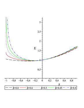
Figure 1: Plot of the dimensionless Hubble rate $E$ against the redshift $z$ for the normal branch ($0.43<\beta$) and for the self-accelerating branch ($\beta<0.43$). The cosmological parameters are assumed to be $\Omega_{m}=0.27$ and $q_{0}=-0.7$. The plot has been done for several values of the holographic parameter $\beta$ that are stated at the bottom of the figure.

As we know, the universe is currently accelerating, i.e. $q_{0}<0$. Hence, using Eqs. (8) and (9) (for $\alpha=0$), we obtain

$$0<\beta=\frac{1-\Omega_{m}-2\epsilon\sqrt{\Omega_{rc}}}{1-q_{0}}<\Omega_{\mathrm{H}_{0}}.$$ (12)

This inequality is quite enlightening and implies an upper or a lower bound on the allowed values of $\beta$ depending on which DGP branch we are considering:

$$\left\{\begin{array}[]{c}\beta<\beta_{\mathrm{lim}}\text{ for \ \ }\epsilon=+1,\\ \beta>\beta_{\mathrm{lim}}\text{ \ for \ }\epsilon=-1,\end{array}\right.$$ (13)

where

$$\beta_{\mathrm{lim}}=\frac{1-\Omega_{m}}{1-q_{0}}.$$ (14)

We can estimate such a bound, $\beta_{\mathrm{lim}}$, taking into account the latest WMAP7 data Komatsu:2010fb and considering that our model does not deviate too much from the $\Lambda$CDM scenario at the present time; i.e. $\Omega_{m}\sim 0.27$ and $q_{0}\sim-0.7$, and so we get a threshold value $\beta_{\mathrm{lim}}\sim 0.43$. From now on, for a given value of $\beta$, we know with which DGP branch we are dealing with, depending on whether $\beta$ is smaller or larger than $0.43$.

As we mentioned at the end of Sect. II, it is not at all obvious how to solve analytically the Friedmann equation (6), even in the simplest case ($\alpha=0$). We will, therefore, analyse the asymptotical solutions of Eq. (6) and combine them with numerical solutions of the same equation. In addition, this analysis is very important to analyse the asymptotical behaviour of the brane and the possible occurrence of any doomsday in the future.

In the far future $(z\rightarrow-1)$, the energy density of matter $\rho_{m}=\rho_{m_{0}}(1+z)^{3}$ is practically zero, and the universe converges asymptotically to a universe filled exclusively with an holographic RDE component.

In the absence of matter, we distinguish two cases for the solutions of equation (6) with $\alpha=0$:

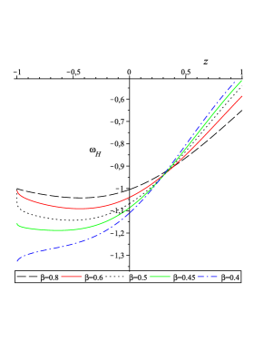
Figure 2: Plot of the equation of state parameter $\omega_{{}_{\mathrm{H}}}$ against the redshift $z$ for the normal branch ($0.43<\beta$) and for the self-accelerating branch ($\beta<0.43$). The cosmological parameters are assumed to be $\Omega_{m}=0.27$ and $q_{0}=-0.7$. The plot has been done for several values of the holographic parameter $\beta$ that are stated at the bottom of the figure.

III.1 Asymptotic behaviour  $\beta=1/2$

We restrict our analysis to expanding branes. Therefore, there is a unique solution supported by the normal branch as implied by the inequalities (13):

$$E=4\sqrt{\Omega_{rc}}x+\mathcal{C}_{1},$$ (15)

where $\mathcal{C}_{1}$ is an integration constant. The solution (15) can be further integrated over time

$$x= \frac{1}{4\sqrt{\Omega_{r_{c}}}}\left\{(4\sqrt{\Omega_{r_{c}}}x_{1}+\mathcal{C}_{1})\times\right.$$ (16)

$$\qquad\quad\left.\exp\left[4\sqrt{\Omega_{r_{c}}}H_{0}(t-t_{1})\right]-\mathcal{C}_{1}\right\},$$

where $x_{1}$ and $t_{1}$ are integration constants. Consequently, in the far future, the scale factor (or $x$) and the Hubble rate diverge. What about $\dot{H}$? It can be easily shown that

$$\frac{dE}{dt}=4\sqrt{\Omega_{r_{c}}}H,$$ (17)

and therefore the cosmic derivative of the Hubble rate also diverges. This kind of event has been named recently a little rip Frampton:2011sp and was previously found on a 4D model Stefancic:2004kb and also on a dilatonic brane-world model BouhmadiLopez:2005gk . In the latter case, the event was called a big rip singularity sent towards an infinite future cosmic time BouhmadiLopez:2005gk .

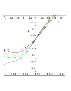
Figure 3: Plot of the deceleration parameter $q$ against the redshift $z$ for the normal branch ($0.43<\beta$) and for the self-accelerating branch ($\beta<0.43$). The cosmological parameters are assumed to be $\Omega_{m}=0.27$ and $q_{0}=-0.7$. The plot has been done for several values of the holographic parameter $\beta$ that are stated at the bottom of the figure.

III.2 Asymptotic behaviour  $\beta\neq 1/2$

The solutions can be expressed as:

$$\arrowvert\frac{2\beta-1}{\beta}E+2\epsilon\frac{\sqrt{\Omega_{r_{c}}}}{\beta}\arrowvert= |\frac{2\beta-1}{\beta}E_{1}+2\epsilon\frac{\sqrt{\Omega_{r_{c}}}}{\beta}|$$

$$\exp\left[-\frac{2\beta-1}{\beta}(x-x_{1})\right],$$

where $E_{1}$ and $x_{1}$ are integration constants, and can be split in two subsets:

III.2.1    $1/2<\ \beta$

This set of values for $\beta$ corresponds to the normal branch as discussed just after Eq. (13), and the dimensionless Hubble rate takes the solution

$$E_{+}=\frac{2\sqrt{\Omega_{rc}}}{\left(2\beta-1\right)}$$ (19)

and becomes asymptotically de Sitter in the far future.

III.2.2
 $\ \ \ \ \beta<1/2$

This case can correspond to any of the two DGP branches (please see the argument given just after Eq. (13)). The dimensionless Hubble rate blows up in the far future at a finite future cosmic time, and it follows a super-accelerated expansion until it hits a big rip singularity bigrip ; Nojiri:2005sx .

III.3 Numerical analysis

Now we return to the equation (6) with $\alpha=0$, in order to solve it and to study the behaviour of the holographic Ricci dark energy. As already mentioned, this equation has no analytical solutions, and a numerical analysis is required. We show our results in Figs. 1, 2 and 3.

In order to solve numerically Eq. (6), we choose $\Omega_{m}\sim 0.27$ and $q_{0}\sim-0.7$, as given by the latest WMAP7 data Komatsu:2010fb and assuming that our model is very similar to the $\Lambda$CDM scenario at the present time. For a given value of $\beta$, the dimensionless energy density $\Omega_{\mathrm{H}_{0}}$ is fixed through Eq. (10), while the crossover scale parameter $\Omega_{r_{c}}$ is fixed by the constraint equation (8).

In Fig. 1, we show five solutions of Eq. (6) corresponding to different values of $\beta$. All the solutions start with a big bang singularity while their behaviour in the future depends strongly on the values acquired by $\beta$ (cf. Fig. 1): for $\beta=0.4$ and $\beta=0.45,$ the brane hits a big rip singularity in the future, for $\beta=0.5$ the brane expands during an infinite time until it reaches a little rip, and finally for $\beta=0.6$ and $\beta=0.8$ the brane is asymptotically de Sitter in the future and the dimensionless Hubble rate $E$ approaches the value $E_{+}=\frac{\beta(1-q_{0})-1+\Omega_{m}}{\left(2\beta-1\right)}$ (see Eq. (19)). All these numerical solutions are in agreement with our analytical analysis as should be.

Even though we have already imposed that the brane is currently accelerating, more precisely we imposed $q_{0}\sim-0.7$, it is important to analyse the behaviour of the equation of state parameter, $\omega_{\mathrm{H}}=p_{\mathrm{H}}/\rho_{\mathrm{H}}$, and the deceleration parameter, $q$, as functions of the redshift. Using the equation of conservation of the Ricci holographic dark energy (HDE),

$$\dot{\rho}_{\mathrm{H}}+3H(\rho_{\mathrm{H}}+p_{\mathrm{H}})=0,$$ (20)

we obtain

$$\omega_{\mathrm{H}}=-1-\frac{1}{3}\frac{d\ln\Omega_{\mathrm{H}}}{dx},$$ (21)

$\Omega_{\mathrm{H}}$ is defined in equation (5). In terms of the dimensionless Hubble rate $E$ and its derivatives with respect to $x$, $\omega_{\mathrm{H}}$ can be rewritten as:

$$\omega_{\mathrm{H}}=-1-\dfrac{\left(\dfrac{dE}{dx}\right)^{2}+E\dfrac{d^{2}E}{dx^{2}}+4E\dfrac{dE}{dx}}{3E\dfrac{dE}{dx}+6E^{2}}$$ (22)

In Fig. 2, we show an example of the behaviour of the equation of state parameter, $\omega_{\mathrm{H}}$, for the current cosmological values, and for different values of $\beta$.

At very late-time $\omega_{\mathrm{H}}$ approaches $-1$ for $\beta\ >1/2$ and tends to $\frac{1}{3}\frac{\beta-2}{\beta}$ for $\beta\ \leq 1/2$ as can be clearly proved from Eq. (15) and Eq. (III.2). We would like to highlight in this regard the smooth transition on the values of $\beta$ when going from an asymptotically de Sitter brane ($1/2<\beta$) to a little rip ($\beta=1/2$) to finally a big rip ($\beta<1/2$). In addition, in this model we can see the little rip as a division between an asymptotically de Sitter universe and a universe approaching/hitting a big rip singularity.

On the other hand, one can prove that for all values of $\beta$ the equation of state of dark energy will evolve in the future in the region $\omega_{\mathrm{H}}\leq-1.$ In addition, using equations (6) and (22), the parameter $\omega_{\mathrm{H}}$ can be expressed at the present time as:

$$\omega_{\mathrm{H}_{0}}=-\frac{\allowbreak\left[\beta\left(q_{0}-1\right)-\Omega_{m}\right](q_{0}-2)-(1+q_{0})\allowbreak}{3\beta(1-q_{0})}.$$ (23)

From the current observational data and from (11) we can assume that $\beta\leq 0.73,$ which means that $\omega_{\mathrm{H}_{0}}<-1,$ and the Ricci dark energy has a phantom-like behaviour. For $\beta>0.5,$ this behaviour will continue in the future and will be more and more like a cosmological constant such that ultimately the universe will enter a de Sitter phase in the far future. For $\beta\leq 0.5$ the behaviour of the Ricci HDE will be phantom-like until the brane reaches a big rip or a little rip. This behaviour is not consistent with the holographic principle which prohibits the occurrence of a big rip singularity Zhang . This motivates us, as was already done in the case of an holographic dark energy with UV cutoff $L=H^{-1}$ preparation , to introduce a GB term in the bulk to try to remove this singularity.

Similarly we can plot the deceleration parameter $q$ against the redshift $z$ for different values of $\beta,$ and for the current cosmological values. The curves in Fig. 3 show that our universe has entered a phase of accelerated expansion in the recent past. The deceleration parameter reaches at very late-time the value $-1$ for $1/2\leq\beta,$ and the value $\frac{\beta-1}{\beta}$ for $\beta<1/2.$

IV Holographic Ricci dark energy in a DGP brane-world with a Gauss-Bonnet term in the bulk

We consider now the model where the bulk action contains a Gauss-Bonnet (GB) curvature term in order to analyse the possibility of avoiding the little rip and big rip present in the absence of such a term. Our motivation in including this curvature modification is based on the fact that a GB curvature term corresponds to an ultra-violet correction to gravity and therefore can influence the high energy regime where both the little rip and big rip take place.

By combining the expressions (8) and (10), we obtain:

$$\epsilon\sqrt{\Omega_{r_{c}}}=\frac{1-\Omega_{m}-\beta(1-q_{0})}{2(1+\Omega_{\alpha})}.$$ (24)

Therefore, the right hand side (rhs) of the previous equality is positive for the self-accelerating branch ($\epsilon=1$) and negative for the normal branch ($\epsilon=-1$). Consequently, there is a limiting allowed value for $\beta$, given by $\beta_{\mathrm{\lim}}$ and defined in Eq. (14), depending on which branch we are considering such that the inequality (13) still holds. Following the same procedure introduced in Sect. III, we conclude that $\beta_{\mathrm{\lim}}\sim 0.43$. In summary, a value of $\beta$ such that $\beta<0.43$ corresponds to the self-accelerating branch, while a value of $\beta$ such that $0.43<\beta$ corresponds to the normal branch.

We would like to highlight that this model has two free parameters: for example $\Omega_{\alpha}$ and $\beta$. Indeed, for a given set of values ($\Omega_{\alpha}$,$\beta$), the model is fully defined because $\Omega_{m}$ is fixed by observations, $\Omega_{\mathrm{H_{0}}}$ is determined by Eq. (10) and $\Omega_{r_{c}}$ by Eq. (24). In our reasoning we have assumed that the $\Lambda$CDM scenario is a good approximation of our model at the present time and we have used the latest WMAP7 data Komatsu:2010fb .

With the inclusion of a GB term in the bulk, it is even less obvious how to solve analytically the Friedmann equation (3). We will, therefore, analyse the asymptotical solutions of Eq. (3) (or equivalently Eq. (6)) and combine them with numerical solutions of the same equation. This analysis will clarify the possible avoidance of a doomsday, of the kind of big rip or little rip, present on the same scenario without GB effects for a set of values of $\beta$.

In the far future $(z\rightarrow-1)$, the energy density of matter $\rho_{m}=\rho_{m_{0}}(1+z)^{3}$ can be neglected, and the universe converges asymptotically to a universe filled exclusively with an holographic RDE component.

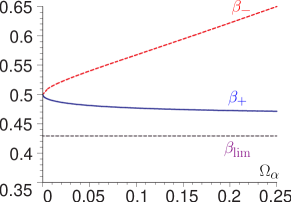
Figure 4: Plot of the parameters $\beta_{\pm}$ and $\beta_{\mathrm{lim}}$, defined in Eqs. (28) and (14), respectively, versus the parameter $\Omega_{\alpha}$. We have used the current observational data $q_{0}\sim-0.7,$ and $\Omega_{m}\sim 0.27$. The parameter $\beta_{\mathrm{lim}}$ defines the border line between the normal branch ($\beta_{\mathrm{lim}}<\beta$) and the self-accelerating branch ($\beta<\beta_{\mathrm{lim}}$). For a given value of $\beta$, the parameters $\beta_{\pm}$ fix the sign of the discriminant $\mathcal{D}$ (cf. Eq. (27)).

IV.1 Asymptotic behaviour

In the absence of matter, the modified Friedmann equation (6) can be rewritten as:

$$\beta\dfrac{dE}{dx}=-\left[{\left(2\beta-1\right)E+2\epsilon\sqrt{\Omega_{rc}}(1+\Omega_{\alpha}E^{2})}\right],$$ (25)

whose solution depends on the sign of the discriminant $\mathcal{D}$ of the polynomial on the rhs, which reads

$$\mathcal{D}=\left(2\beta-1\right)^{2}-16\Omega_{r_{c}}\Omega_{\alpha}.$$ (26)

It is convenient to factorise the discriminant $\mathcal{D}$ as follows

$$\mathcal{D}=\mathcal{F}(\beta-\beta_{-})(\beta-\beta_{+}).$$ (27)

where

$$\beta_{\pm} = \frac{1+\Omega_{\alpha}\pm 2\sqrt{\Omega_{\alpha}}(1-\Omega_{m})}{2\left[1+\Omega_{\alpha}\pm\sqrt{\Omega_{\alpha}}(1-q_{0})\right]},$$ (28)

$$\mathcal{F} = 4\left[1-\Omega_{\alpha}\left(\frac{1-q_{0}}{1+\Omega_{\alpha}}\right)^{2}\right].$$ (29)

We show in Fig. 4, the shape of $\beta_{\pm}$ for physically reasonable values of $\Omega_{\alpha}$. It can be shown as well that for the same range of values of $\Omega_{\alpha}$, the coefficient $\mathcal{F}$ is positive (see Eq. (29)). Therefore, the discriminant $\mathcal{D}$ is positive when $\beta<\beta_{+}$ or $\beta_{-}<\beta$, negative for $\beta_{+}<\beta<\beta_{-}$ and vanishes for $\beta=\beta_{+},\beta_{-}$. We next tackle each of these cases separately.

IV.1.1 Negative discriminant ($\mathcal{D}<0$)

The discriminant $\mathcal{D}$ is negative when $\beta$ satisfies $\beta_{+}<\beta<\beta_{-}$ (cf. Eq. (27) and Fig. 4). As $\beta_{\mathrm{lim}}<\beta_{+}$ this case can take place only for the normal branch and the Friedmann equation (25) can be integrated as:

$$E=\frac{1}{4\Omega_{\alpha}\sqrt{\Omega_{rc}}}\left\{\sqrt{\left|\mathcal{D}\right|}\tan\left[\frac{\sqrt{\left|\mathcal{D}\right|}}{2\beta}\left(x-\mathcal{C}_{2}\right)\right]+2\beta-1\right\},$$ (30)

where

$$\mathcal{C}_{2}=x_{2}+\frac{2\beta}{\sqrt{\left|\mathcal{D}\right|}}\arctan\left[\frac{-4\Omega_{\alpha}\sqrt{\Omega_{r_{c}}}E_{2}+2\beta-1}{\sqrt{\left|\mathcal{D}\right|}}\right],$$ (31)

and $x_{2}$ and $E_{2}$ are integration constants. Consequently, there is always a finite value of the scale factor or $x$ where the Hubble rate blows up:

$$x_{\mathrm{sing_{1}}}=\mathcal{C}_{2}+\frac{2\beta}{\sqrt{\left|\mathcal{D}\right|}}(n+\frac{1}{2})\pi,\quad n\in\mathbb{Z}.$$ (32)

The singularity takes place at $x_{\mathrm{sing}}$ for an integer $n$ such that $x_{\mathrm{sing_{1}}}$ takes the smallest possible positive value. Not only the Hubble rate but also its cosmic derivative blow up at $x_{\mathrm{sing_{1}}}$ (see Eq. (7)). Finally, integrating the dimensionless Hubble rate (30) with respect to time we obtain

$$\sqrt{\left|\mathcal{D}\right|}\ln\left\{\frac{\sqrt{\left|\mathcal{D}\right|}\tan\left[\frac{\sqrt{\left|\mathcal{D}\right|}}{2\beta}\left(x-\mathcal{C}_{2}\right)\right]+2\beta-1}{\sqrt{1+\tan^{2}\left[\frac{\sqrt{\left|\mathcal{D}\right|}}{2\beta}\left(x-\mathcal{C}_{2}\right)\right]}}\right\}+2\beta-1$$ (33)

$$\quad=\frac{H_{0}\left[\left|\mathcal{D}\right|+(2\beta-1)^{2}\right]}{4\Omega_{\alpha}\sqrt{\Omega_{r_{c}}}}(t-t_{\mathrm{sing_{1}}}),$$

concluding therefore that the brane hits a big freeze singularity in the future as the event $x_{\mathrm{sing_{1}}}$ takes place at a finite future cosmic time $t_{\mathrm{sing_{1}}}$ Nojiri:2005sx ; BouhmadiLopez:2006fu .

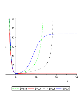
Figure 5: Plot of the dimensionless Hubble rate $E$ against $x$ for the normal branch ($0.43<\beta$) and for the self-accelerating branch ($\beta<0.43$). The cosmological parameters are assumed to be $\Omega_{m}=0.27$ and $q_{0}=-0.7$. The plot has been done for several values of the holographic parameter $\beta$ that are stated at the bottom of the figure. The reason we show this plot in terms of $x$, rather than $z$, is to see clearly the presence of a big freeze singularity for some values of $\beta$.

IV.1.2 Positive discriminant ($0<\mathcal{D}$)

The discriminant $\mathcal{D}$ is positive when $\beta<\beta_{+}$ or $\beta_{-}<\beta$ (cf. Eq. (27) and Fig. 4) which can take place either on the normal branch ($\beta>\beta_{\mathrm{lim}}$) or the self-accelerating branch ($\beta_{\mathrm{lim}}>\beta$).

The solution of the asymptotic Friedmann equation (25) reads:

$$\left|\frac{4\epsilon\Omega_{\alpha}\sqrt{\Omega_{r_{c}}}\,E+2\beta-1-\sqrt{\mathcal{D}}}{4\epsilon\Omega_{\alpha}\sqrt{\Omega_{r_{c}}}\,E+2\beta-1+\sqrt{\mathcal{D}}}\right|=\mathcal{C}_{2}\exp\left[-\frac{\sqrt{\mathcal{D}}}{\beta}(x-x_{2})\right],$$ (34)

where

$$\mathcal{C}_{2}=\left|\frac{4\epsilon\Omega_{\alpha}\sqrt{\Omega_{r_{c}}}\,E_{2}+2\beta-1-\sqrt{\mathcal{D}}}{4\epsilon\Omega_{\alpha}\sqrt{\Omega_{r_{c}}}\,E_{2}+2\beta-1+\sqrt{\mathcal{D}}}\right|,$$ (35)

$x_{2}$ and $E_{2}$ are integration constants. We can then deduce that the brane expands till it reaches an infinite size; i.e. for very large values of $x$, if and only if the brane is asymptotically de Sitter with Hubble rate

$$E_{+}=\frac{\sqrt{\mathcal{D}}-(2\beta-1)}{4\epsilon\Omega_{\alpha}\sqrt{\Omega_{r_{c}}}}.$$ (36)

Notice that ${E_{+}}$ reduces to Eq. (19) in absence of GB effects in the bulk. The brane can be asymptotically de Sitter only in too cases: (i) For $\epsilon=1$ as $\beta<\beta_{\mathrm{lim}}<\frac{1}{2}$ and (ii) for $\epsilon=-1$ if $\frac{1}{2}<\beta_{-}<\beta$. In both cases the Hubble rate $E_{+}$ is a positive constant.

What happens in the remaining case; i.e. $\epsilon=-1$ and $\beta_{\mathrm{lim}}<\beta<\beta_{+}$? In the latter case $E_{+}$ is negative and the asymptotic analysis performed is no longer valid. In fact, the brane faces a big freeze singularity in this situation where the expansion of the brane can be approximated by

$$E\sim\frac{1}{2\Omega_{\alpha}\sqrt{\Omega_{r_{c}}}\,(x_{\mathrm{sing_{2}}}-x)}.$$ (37)

The constant $x_{\mathrm{sing_{2}}}$ stands for the “size” of the brane at the big freeze singularity. The Hubble rate (37) can be integrated over time, resulting in the following expansion for the scale factor of the brane

$$a=a_{\mathrm{sing_{2}}}\exp\left[-\left(\frac{H_{0}}{2\Omega_{\alpha}\sqrt{\Omega_{r_{c}}}}\right)^{\frac{1}{2}}\sqrt{t_{\mathrm{sing_{2}}}-t}\right]$$ (38)

The big freeze singularity takes place at a finite scale factor, $a_{\mathrm{sing_{2}}}$, and a finite cosmic time, $t_{\mathrm{sing_{2}}}$.

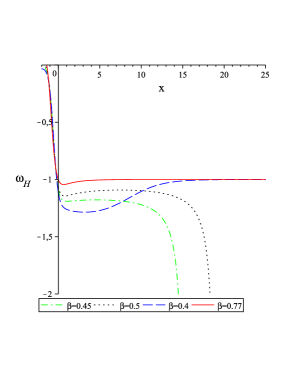
Figure 6: Parameter $\omega_{{}_{\mathrm{H}}}$ against $x$ for the normal branch ($0.43<\beta$) and for the self-accelerating branch ($\beta<0.43$). The cosmological parameters are assumed to be $\Omega_{m}=0.27$, $q_{0}=-0.7$ and $\Omega_{\alpha}=0.1$. The plot has been done for several values of the holographic parameter $\beta$ that are stated at the bottom of the figure. The reason we show this plot in terms of $x$, rather than $z$, is to see what are the effects of the big freeze on the equation of state parameter.

IV.1.3 Vanishing discriminant ($\mathcal{D}=0$)

Finally, the discriminant $\mathcal{D}$ vanishes when $\beta=\beta_{+}$ or $\beta_{-}$. This can take place only on the normal branch. In this fine tuned case, the solution of the modified Friedmann equation (25) can be expressed as

$$E=\frac{1}{4\Omega_{\alpha}\sqrt{\Omega_{r_{c}}}}\left[(2\beta-1)-\frac{1}{\mathcal{C}_{2}+\frac{1}{2\beta}(x-x_{2})}\right],$$ (39)

where

$$\mathcal{C}_{2}=\frac{1}{2\beta-1-4\Omega_{\alpha}\sqrt{\Omega_{r_{c}}}E_{2}},$$ (40)

and $x_{2}$ and $E_{2}$ are integration constants. By taking the limit $x\rightarrow\infty$, the dimensionless Hubble rate (39) reduces to

$$E_{+}=\frac{2\beta-1}{4\Omega_{\alpha}\sqrt{\Omega_{r_{c}}}},$$ (41)

Not surprisingly, $E_{+}$ coincides with the one defined in Eq. (36) for vanishing $\mathcal{D}$ on the normal branch. The dimensionless Hubble rate is positive only for values of $\beta$ such that $\beta=\beta_{-}$ where the brane is asymptotically de Sitter. The solution (39) is not valid on the normal expanding branch with $\beta=\beta_{+}$, as the Hubble rate becomes negative, a condition which signals that the asymptotical behaviour given by (39) breaks down. In fact, what happens on the normal branch for $\beta=\beta_{+}$ is that the brane hits a big freeze singularity at a finite scale factor and the brane expansion can be approximated by Eq. (37).

IV.2 Numerical analysis

The asymptotical analysis we have carried out in the previous subsection can be complemented with a numerical analysis. We show some examples of the numerical analysis in Fig 5. More precisely, we obtain:

• If $\beta<\beta_{\mathrm{lim}}$, the solution corresponds to the self-accelerating branch and the brane is asymptotically de Sitter in the future.

• If $\beta_{\mathrm{lim}}<\beta<\beta_{-}$, the solution corresponds to the normal branch and the brane faces a big freeze in the future. Notice that for the case $\beta=1/2$ with $\Omega_{\alpha}\neq 0$ the brane faces a big freeze, while it faces a little rip in the absence of a GB term in the bulk ($\Omega_{\alpha}=0$).

• If $\beta_{-}\leq\beta$, the solution corresponds to the normal branch and is asymptotically de Sitter in the future.

In summary, we conclude that the big rip that might show up on the self-accelerating branch without GB effects in the bulk is removed by the inclusion of GB effects in the bulk. However, the situation in the normal branch is quite different as the presence of the GB effects, even though they remove the big rip and little rip, it cannot always prevent the presence of a big freeze singularity in the future evolution of the brane.

For completeness, we will discuss the behaviour of the equation of state $\omega_{\mathrm{H}}$ associated with the Ricci HDE. We can show that the function $\omega_{\mathrm{H}}$ approaches $-1$ at very late-time, in the case where the brane is asymptotically de Sitter, while it diverges to minus infinity when the brane face a big freeze singularity in the future (see also Fig. 6). In addition, we can show by using equations (6) and (22), that the equation of state parameter $\omega_{\mathrm{H}}$ can be expressed at the present time as:

$$\omega_{\mathrm{H}_{0}}=$$

$$\frac{\allowbreak\left[\beta(1-q_{0})+\Omega_{m}\right]\left[q_{0}(1+3\Omega_{\alpha})-2\right]-(1+q_{0})\allowbreak\left(\Omega_{\alpha}-1\right)}{3\beta(1-q_{0})(\Omega_{\alpha}+1)}.$$

Fig. 7 shows the variation of $\omega_{\mathrm{H}_{0}}$ with respect to $\Omega_{\alpha}$ and $\beta,$ where we have used the current values of $q_{0}\sim-0.7$ and $\Omega_{m}\sim 0.27.$ The figure shows that $\omega_{\mathrm{H}_{0}}$ is always less than $-1/3$ at present. Notice as well that the most likely value of $\beta$ is of the order of $\beta_{-}$ or larger, and therefore the big freeze singularity will be avoided in the future evolution of the brane (cf. Figs. 4 and 7).

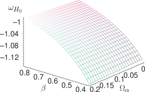
Figure 7: Plot of $\omega_{\mathrm{H}_{0}}$ against $\beta$ and $\Omega_{\alpha}$ . The cosmological parameters are assumed to be $\Omega_{m}=0.27$ and $q_{0}=-0.7$.

One can conclude that for all values of $\Omega_{\alpha}$ and $\beta,$ the equation of state of dark energy $\omega_{\mathrm{H}}$ will evolve at future in the region $\omega_{\mathrm{H}}<-1/3,$ and converges to $-1$ or minus infinity as discussed above. Fig. 6 illustrates the case of $\ \Omega_{\alpha}=0.1$. This figure shows that the curve of $\omega_{\mathrm{H}}$ crosses currently the boundary of the cosmological constant $\omega_{\mathrm{H}}=-1$ for $\beta_{\mathrm{0}}\sim 0.77,$ while for $\beta<\beta_{\mathrm{0}}$ the equation of state of dark energy will evolve as a phantom-like fluid, i.e. $\omega_{\mathrm{H}}<-1$. This behaviour will manifest itself more and more in the future until ending with a big freeze for $\beta_{\mathrm{\lim}}{<}\beta<\beta_{-}$, and with a de Sitter-like universe for $\beta<\beta_{\mathrm{\lim}}$ and $\beta_{-}\leq\beta$.

We note here that according to Eq. (11) $\beta$ is always less than $\beta_{\mathrm{0}}$ and the nature of the Ricci dark energy has always a phantom-like behaviour.

Once again one can test this model by plotting the deceleration parameter $q$ versus the redshift for some values of $\beta$. Fig. 8 shows that our universe is currently in an accelerating expansion phase.

V Conclusions

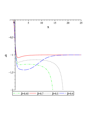
Figure 8: Plot of the deceleration parameter against $x$ for the normal branch ($0.43<\beta$) and for the self-accelerating branch ($\beta<0.43$). The cosmological parameters are assumed to be $\Omega_{m}=0.27$, $q_{0}=-0.7$ and $\Omega_{\alpha}=0.1$. The plot has been done for several values of the holographic parameter $\beta$ that are stated at the bottom of the figure. The reason we show this plot in terms of $x$, rather than $z$, is to see what are the effects of the big freeze on the decceleration parameter.

In this paper we have considered an holographic DGP brane-world model with the average radius of the Ricci scalar curvature as an infrared cutoff. We have shown that the late-time acceleration of the Universe with and without the Gauss-Bonnet (GB) term in the bulk, is consistent with the current observational data.

The Ricci HDE is characterised by the parameter $\beta$ (see Eq. (2)) which is bounded by the current value of the dimensionless Ricci HDE $\Omega_{\mathrm{H}_{0}}$ (cf. Eq. (11)). In addition, there is a limiting value of $\beta$, which we named $\beta_{\mathrm{lim}}$ (see Eqs. (13) and (14)) that splits the allowed $\beta$ values for the self-accelerating branch ($\epsilon=1$) from the normal branch ($\epsilon=-1$). More precisely, values of $\beta$ such that $\beta<\beta_{\mathrm{lim}}$ correspond to the self-accelerating branch while values of $\beta$ such that $\beta_{\mathrm{lim}}<\beta$ corresponds to the normal branch. We can estimate that $\beta_{\mathrm{lim}}\sim 0.43$ assuming that our model does not deviate too much from the $\Lambda$CDM model at present. The value acquired by $\beta$ is very important in determining the asymptotical behaviour of the brane and that of the Ricci HDE.

In the absence of GB effects, the equation of state of the Ricci HDE will evolve in the region $\omega_{\mathrm{H}}<-1$ and its late-time behaviour is phantom-like with two distinct destinies of the universe: (i) for $1/2<\beta$, corresponding exclusively to the normal branch, this phantom-like behaviour will be more and more like a cosmological constant in the far future and the brane expansion is asymptotically de Sitter. In this case, the normal branch does not require the inclusion of a GB term in the bulk to remove any singularity in the far future. (ii) for $\beta\leq 1/2$ (self-accelerating or normal branch), this phantom-like behaviour continues and implies a super-accelerated expansion on the brane leading to a big rip or a little rip singularity. These sets of solutions may require a GB term in order to remove or smooth those singularities. This is what motivates us to consider a GB correction in the bulk.

The introduction of a GB term in the bulk may remove the big rip and little rip from the future evolution of the brane. In the self-accelerating branch the brane becomes asymptotically de Sitter, however, the normal branch can hit a big freeze singularity in the far future. More precisely, the normal branch is asymptotically de Sitter for $\beta_{-}<\beta$ and hits a big freeze singularity when $\beta_{\mathrm{lim}}\leq\beta<\beta_{-}$ (see Eqs. (28), (4.7) and (37)). The Ricci HDE has a phantom-like behaviour which either approaches a de Sitter-like state or induces a big freeze as explained above. The case corresponding to a big freeze singularity is quite unlikely because it leads to a quite negative equation of state at present (please see Figs. 4 and 7). At this regard, we would like to stress that an observationally consistent value of the equation of state (EOS) parameter of the Ricci HDE is even more important than the GB parameter to reject the parameter region where the future singularity appears. In fact, even in the absence of a GB parameter, the EOS parameter already pick up a singularity free region (cf. Fig. 2). Then what is the role of the GB term? it narrows the region affected by the singularity if $\beta\leq 1/2$ (with respect to the model without a GB term) and enlarges that region if $1/2\leq\beta$ (with respect to the model without a GB term).

In summary, it is always possible to construct a Ricci HDE brane-world model consistent with current observations. The brane with or without GB effects is always free of future singularities except for the range of values of $\beta$ such that $\beta_{\rm{lim}}\leq\beta\leq 1/2$ which happens always in the normal branch. However, these values are very unlikely (cf. Figs. 4 and 7) because they lead to a very negative equation of state at the present as explained above.

This study opens a new way of considering interactions between dark matter and the holographic dark energy. We hope to report this issue in a forthcoming publication preparation2 .

- (1) S. Perlmutter et al., Astrophys. J. 517, 565 (1999) [arXiv:astro-ph/9812133]. A. G. Riess et al., Astron. J. 116, 1009 (1998) [arXiv:astro-ph/9805201]. M. Kowalski et al., Astrophys. J. 686, 749 (2008) [arXiv:0804.4142 [astro-ph]].
- (2) D. N. Spergel et al.,Astrophys. J. Suppl. 148, 175 (2003) [arXiv:astro-ph/0302209]; ibid. Astrophys. J. Suppl. 170, 377 (2007) [arXiv:astro-ph/0603449]; E. Komatsu et al. [WMAP Collaboration], Astrophys. J. Suppl. 180, 330 (2009) [arXiv:0803.0547 [astro-ph]].
- (3) M. Tegmark, et al., SDSS Collaboration, Phys. Rev. D 69, 103501 (2004)[arXiv:astro-ph/0310723]; J.K. Adelman-McCarthy, et al., SDSS Collaboration, Astrophys. J. Suppl. 175, 297 (2008) [arXiv:0707.3413 [astro-ph]].
- (4) P.J.E. Peebles and B. Ratra, Rev. Mod. Phys. 75, 559 (2003) [astro-ph/0207347].
- (5) B. Ratra and P.J.E. Peebles, Phys. Rev. D 37, 3406 (1988); I. Zlatev, L. Wang and P.J. Steinhardt, Phys. Rev. Lett. 82, 896 (1999).
- (6) Amendaiz-Picon, Phys. Rev. D 63, 103510 (2001).
- (7) R.R. Caldwell, Phys. Lett. B 545, 23 (2002); S.M. Carroll, M. Hoffman and M. Trodden, Phys. Rev. D 68, 023509 (2003); J. G. Hao, X. Z. Li, Phys. Rev. D 68, 043501 (2003); D. J. Liu, X. Z. Li, Phys. Rev. D 68, 067301 (2003).
- (8) G. ’t Hooft, arXiv:gr-qc/9310026.
- (9) L. Susskind, J. Math. Phys. 36, 6377 (1995) [arXiv:hep-th/9409089].
- (10) A. G. Cohen, D. B. Kaplan and A. E. Nelson, Phys. Rev. Lett. 82, 4971 (1999) [arXiv:hep-th/9803132].
- (11) M. Li, Phys. Lett. B 603, 1 (2004) [arXiv:hep-th/0403127].
- (12) S. D. H. Hsu, Phys. Lett. B 594, 13 (2004) [arXiv:hep-th/0403052].
- (13) X. Wu, R. G. Cai and Z. H. Zhu, Phys. Rev. D 77, 043502 (2008) [arXiv:0712.3604 [astro-ph]].
- (14) M. Bouhmadi-López, A. Errahmani and T. Ouali, Phys. Rev. D 84, 083508 (2011) [arXiv:1104.1181 [astro-ph.CO]].
- (15) E. N. Saridakis, Phys. Lett. B 660, 138 (2008) [arXiv:0712.2228 [hep-th]]; ibid JCAP 0804, 020 (2008) [arXiv:0712.2672 [astro-ph]]; ibid Phys. Lett. B 661, 335 (2008) [arXiv:0712.3806 [gr-qc]].
- (16) C. Gao, F.Q. Wu, X. Chen, Y.G. Shen, Phys. Rev. D 79, 043511 (2009) [arXiv: 0712.1394 [astro-ph]].
- (17) S. ’i. Nojiri and S. D. Odintsov, Gen. Rel. Grav. 38, 1285 (2006) [hep-th/0506212].
- (18) G. R. Dvali, G. Gabadadze, M. Porrati, Phys. Lett. B484, 112 (2000) [hep-th/0002190]; ibid. Phys. Lett. B485, 208 (2000) [hep-th/0005016].
- (19) C. Deffayet, Phys. Lett. B 502, 199 (2001) [arXiv:hep-th/0010186].
- (20) V. Sahni and Y. Shtanov, JCAP 0311, 014 (2003) [arXiv:astro-ph/0202346]; L. P. Chimento, R. Lazkoz, R. Maartens, I. Quiros, JCAP 0609, 004 (2006) [astro-ph/0605450]; H. S. Zhang and Z. H. Zhu, Phys. Rev. D 75, 023510 (2007) [arXiv:astro-ph/0611834]; M. Bouhmadi-López, R. Lazkoz, Phys. Lett. B654, 51-57 (2007). [arXiv:0706.3896 [astro-ph]].
- (21) M. Bouhmadi-López, JCAP 0911, 011 (2009) [arXiv:0905.1962 [hep-th]]; M. Bouhmadi-López, S. Capozziello, V. F. Cardone, Phys. Rev. D82, 103526 (2010) [arXiv:1010.1547].
- (22) G. Kofinas, R. Maartens and E. Papantonopoulos, JHEP 0310, 066 (2003) [arXiv:hep-th/0307138].
- (23) R. A. Brown, R. Maartens, E. Papantonopoulos and V. Zamarias, JCAP 0511, 008 (2005) [arXiv:gr-qc/0508116]; R. A. Brown, Gen. Rel. Grav. 39, 477 (2007) [arXiv:gr-qc/0602050]; R. G. Cai, H. S. Zhang and A. Wang, Commun. Theor. Phys. 44, 948 (2005) [arXiv:hep-th/0505186].
- (24) M. Bouhmadi-López and P. V. Moniz, Phys. Rev. D 78, 084019 (2008) [arXiv:0804.4484 [gr-qc]]; M. Bouhmadi-López, Y. Tavakoli and P. V. Moniz, JCAP 1004, 016 (2010) [arXiv:0911.1428 [gr-qc]].
- (25) Chao-Jun Feng and Xin Zhang Phys. Lett. B 680, 399 (2009) [arXiv:gr-qc/0904.0045v3].
- (26) Y. Shtanov and V. Sahni, Class. Quant. Grav. 19, L101 (2002) [gr-qc/0204040].
- (27) J. D. Barrow, Class. Quant. Grav. 21, L79 (2004) [gr-qc/0403084].
- (28) S. Nojiri, S. D. Odintsov and S. Tsujikawa, Phys. Rev. D 71, 063004 (2005) [arXiv:hep-th/0501025].
- (29) C. Cattoën and M. Visser, Class. Quant. Grav. 22, 4913 (2005) [arXiv:gr-qc/0508045]; L. Fernández-Jambrina and R. Lazkoz, Phys. Rev. D 74, 064030 (2006) [arXiv:gr-qc/0607073].
- (30) R. R. Caldwell, Phys. Lett. B 545, 23 (2002) [arXiv:astro-ph/9908168]; A. A. Starobinsky, Grav. Cosmol. 6, 157 (2000) 157 [arXiv:astro-ph/9912054]; S. M. Carroll, M. Hoffman and M. Trodden, Phys. Rev. D 68, 023509 (2003) [arXiv:astro-ph/0301273]; R. R. Caldwell, M. Kamionkowski and N. N. Weinberg, Phys. Rev. Lett. 91, 071301 (2003) [arXiv:astro-ph/0302506]; M. Bouhmadi-López and J. A. Jiménez Madrid, JCAP 0505, 005 (2005) [astro-ph/0404540]; E. Elizalde, S. ’i. Nojiri and S. D. Odintsov, Phys. Rev. D 70, 043539 (2004) [hep-th/0405034].
- (31) M. Bouhmadi-López, P. F. González-Díaz, P. Martín-Moruno, Phys. Lett. B659, 1 (2008) [gr-qc/0612135]; ibid. Int. J. Mod. Phys. D17, 2269 (2008) [arXiv:0707.2390 [gr-qc]].
- (32) H. Štefančić, Phys. Rev. D71, 084024 (2005) [astro-ph/0411630].
- (33) M. Bouhmadi-López, Nucl. Phys. B797, 78 (2008) [astro-ph/0512124].
- (34) P. H. Frampton, K. J. Ludwick, R. J. Scherrer, Phys. Rev. D84, 063003 (2011) [arXiv:1106.4996 [astro-ph.CO]]; I. Brevik, E. Elizalde, S. Nojiri and S. D. Odintsov, Phys. Rev. D 84, 103508 (2011) [arXiv:1107.4642 [hep-th]]; P. H. Frampton, K. J. Ludwick, S. ’i. Nojiri, S. D. Odintsov and R. J. Scherrer, arXiv:1108.0067 [hep-th]; S. ’i. Nojiri, S. D. Odintsov and D. Sáez-Gómez, arXiv:1108.0767 [hep-th].
- (35) M.-H. Belkacemi, A. Errahmani, and T. Ouali, in preparation.