Low-energy expansion formula for one-dimensional Fokker-Planck and Schrödinger equations with asymptotically periodic potentials

Abstract

We consider one-dimensional Fokker-Planck and Schrödinger equations with a potential which approaches a periodic function at spatial infinity. We extend the low-energy expansion method, which was introduced in previous papers, to be applicable to such asymptotically periodic cases. Using this method, we study the low-energy behavior of the Green function.

1 Introduction

We consider the one-dimensional Fokker-Planck equation

$$-\frac{\rmd^{2}}{\rmd x^{2}}\phi(x)+2\frac{\rmd}{\rmd x}[f(x)\phi(x)]=k^{2}\phi(x)$$ (1.1)

or the equivalent Schrödinger equation

$$-\frac{\rmd^{2}}{\rmd x^{2}}\psi(x)+V_{\rm S}(x)\psi(x)=k^{2}\psi(x).$$ (1.2)

Equation (1.1) describes the diffusion of particles in an external potential $V(x)$, from which the function $f(x)$ in (1.1) is defined by

$$f(x)=-\frac{1}{2}\frac{\rmd}{\rmd x}V(x).$$ (1.3)

The Schrödinger potential $V_{\rm S}$ and the function $\psi$ of (1.2) are are related to $f$ and $\phi$ by

$$V_{\rm S}(x)=f^{2}(x)+f^{\prime}(x)$$ (1.4)

and

$$\phi(x)=\rme^{-V(x)/2}\psi(x).$$ (1.5)

We shall always assume that ${\rm Im}\,k\geq 0$. We define the Green function $G_{\rm S}(x,y;k)$ for the Schrödinger equation as the function satisfying

$$\left[\frac{\partial^{2}}{\partial x^{2}}-V_{\rm S}(x)+k^{2}\right]G_{\rm S}(x,y;k)=\delta(x-y)$$ (1.6)

with the boundary conditions $G_{\rm S}(x,y;k)\to 0$ as $|x-y|\to\infty$ for ${\rm Im}\,k>0$. For ${\rm Im}\,k=0$, we define $G_{\rm S}(x,y;k)\equiv\lim_{\epsilon\downarrow 0}G_{\rm S}(x,y;k+\rm i\epsilon)$. Without loss of generality, we may suppose that $x\geq y$.

In a series of previous papers [1,2], we discussed a method for calculating the expansion of $G_{\rm S}(k)$ in powers of $k$. In [1], we studied the cases in which the potential $V(x)$ either converges to a finite limit of diverges to infinity as $x\to\pm\infty$. In [2], we dealt with periodic potentials satisfying $V(x+L)=V(x)$. In this paper, we shall deal with asymptotically periodic potentials, i.e. potentials $V(x)$ that approach a periodic function as $x\to\pm\infty$. In solid state physics, impurities in a crystal are described by this type of potentials. The study of asymptotically periodic potentials is important for the application in physics, and there is a fair amount of literature on this subject [3-12]. However, there has not yet been a systematic analysis of the the low-energy behavior of the Green function up to high orders in $k$. In this paper, we shall show that the method introduced in [1] and [2] can be extended to the asymptotically periodic case, enabling us to obtain the expansion of the Green function up to any order in $k$.

We assume that the potential $V(x)$ is a real-valued function which is piecewise continuously differentiable. (Note that $V(x)$ may have have jump discontinuities. See footnote 1 of [2] and footnote 1 of [1].) We also assume that $V$ can be expressed as a sum of two functions:

$$V(x)=V_{\rm p}(x)+V_{\Delta}(x),$$ (1.7)

where $V_{\rm p}$ is a periodic function satisfying

$$V_{\rm p}(x+L)=V_{\rm p}(x),$$ (1.8a)

and $$V_{\Delta}$$ is a function such that

$$\lim_{x\to\pm\infty}V_{\Delta}(x)=0.$$ (1.8b)

Corresponding to (1.7), we assume that the function $f$ (equation (1.3)) can be written as

$$f(x)=f_{\rm p}(x)+f_{\Delta}(x),$$ (1.8i)

where $f_{\rm p}(x+L)=f_{\rm p}(x)$ and $\lim_{x\to\pm\infty}f_{\Delta}(x)=0$.

As we will see, the Green function can be expanded in terms of $k$ as

$$G_{\rm S}(x,y;k)=(\rmi k)^{-1}g_{-1}(x,y)+g_{0}(x,y)+\rmi kg_{1}(x,y)+(\rmi k)^{2}g_{2}(x,y)$$

$$+\cdots+(\rmi k)^{N}g_{N}(x,y)+o(k^{N})$$ (1.8j)

if $V_{\Delta}\in L^{1}_{N}$, where $L^{1}_{n}$ denotes the set of functions $v(x)$ satisfying

$$\int_{-\infty}^{\infty}(1+|x|^{n})|v(x)|\,\rmd x<\infty.$$ (1.8k)

In this paper, we shall discuss the method for systematically calculating the coefficients $g_{-1},g_{0},g_{1},\ldots$ of (1.10). Our method is based on the expansion formula for the reflection coefficient, which was derived in [13]. This formula will be reviewed in section 3, after introducing some necessary notations in section 2. The calculation of $g_{n}$ is done in sections 4–9.

It is easy to extend this method to potentials $V(x)$ which have different asymptotic behaviors as $x\to-\infty$ and $x\to+\infty$. For example, we can easily deal with the cases where $V(x)$ approaches periodic functions with different periods as $x\to-\infty$ and $x\to+\infty$. This will be discussed in section 10.

If $V(x)$ is asymptotically periodic, the corresponding $V_{\rm S}(x)$ is also asymptotically periodic. That is to say, if $V$ has the form of (1.7) with (1.8), then $V_{\rm S}$ has the form

$$V_{\rm S}(x)=V_{\rm p}^{\rm S}(x)+V_{\Delta}^{\rm S}(x),\qquad V_{\rm p}^{\rm S}(x+L)=V_{\rm p}^{\rm S}(x),\qquad\lim_{x\to\pm\infty}V_{\Delta}^{\rm S}(x)=0.$$ (1.8l)

But the converse is not necessarily true. Suppose that a Schrödinger potential $V_{\rm S}$ satisfying (1.12) is given. For simplicity, we assume that there are no bound states. Then the corresponding Fokker-Planck potential $V$ satisfies (1.7) and (1.8) only if the wave function $\psi(x)$ at the bottom of the lowest energy band remains finite for both $x\to+\infty$ and $x\to-\infty$. This is what is called the ‘exceptional case’ in the conventional terminology of scattering theory [6]. In the ‘generic case’, the Fokker-Planck potential $V(x)$ corresponding to an asymptotically periodic $V_{\rm S}(x)$ is not asymptotically periodic but tends to $-\infty$ at either $x\to+\infty$ or $x\to-\infty$ (see example 2 in section 12). Our method is also applicable to $V_{\rm S}$ in the generic case, even though such $V_{\rm S}$ does not correspond to a Fokker-Planck potential satisfying (1.7) with (1.8). In the generic case, the expansion of $G_{\rm S}$ begins with the term of order $k^{0}$ (namely, $g_{-1}=0$ in (1.10)). In section 11, we will see how to calculate $g_{0},g_{1},g_{2},\ldots$ for the generic case.

2 Preliminaries

Let the $2\times 2$ matrix $U(x,x^{\prime};k)$ be the solution of

$$\frac{\partial}{\partial x}U(x,x^{\prime};k)=\left(\begin{array}[]{cc}-\rmi k&f(x)\\ f(x)&\rmi k\\ \end{array}\right)U(x,x^{\prime};k),\qquad U(x^{\prime},x^{\prime};k)=\left(\begin{array}[]{cc}1&0\\ 0&1\\ \end{array}\right).$$ (1.8a)

We write the elements of $U$ as

$$U(x,x^{\prime};k)\equiv\left(\begin{array}[]{cc}\alpha(x,x^{\prime};k)&\beta(x,x^{\prime};-k)\\ \beta(x,x^{\prime};k)&\alpha(x,x^{\prime};-k)\\ \end{array}\right),$$ (1.8b)

and define the transmission coefficient $\tau$, the right reflection coefficient $R_{r}$ and the left reflection coefficient $R_{l}$ as

$$\tau(x,x^{\prime};k)\equiv\frac{1}{\alpha(x,x^{\prime};k)},\qquad R_{r}(x,x^{\prime};k)\equiv\frac{\beta(x,x^{\prime};k)}{\alpha(x,x^{\prime};k)},\qquad R_{l}(x,x^{\prime};k)\equiv-\frac{\beta(x,x^{\prime};-k)}{\alpha(x,x^{\prime};k)}.$$

The generalized scattering coefficients $\bar{\tau}$, $\bar{R}_{r}$, $\bar{R}_{l}$ are defined with an additional variable $W$ as

$$\bar{\tau}(x,x^{\prime};W;k)\equiv\frac{\sqrt{1-\xi^{2}}\,\tau(x,x^{\prime};k)}{1-\xi R_{r}(x,x^{\prime};k)},\qquad\bar{R}_{r}(x,x^{\prime};W;k)\equiv\frac{R_{r}(x,x^{\prime};k)-\xi}{1-\xi R_{r}(x,x^{\prime};k)},$$

$$\bar{R}_{l}(x,x^{\prime};W;k)\equiv R_{l}(x,x^{\prime};k)+\frac{\xi\tau^{2}(x,x^{\prime};k)}{1-\xi R_{r}(x,x^{\prime};k)},$$ (1.8e)

where

$$\xi(x,W)\equiv\tanh\frac{W-V(x)}{2}.$$ (1.8f)

(For an alternative definition, see (A.2) and (A.3) of appendix A.) We also define

$$S_{r}(x,k)\equiv\frac{R_{r}(x,-\infty;k)}{1+R_{r}(x,-\infty;k)},\qquad S_{l}(x,k)\equiv\frac{R_{l}(\infty,x;k)}{1+R_{l}(\infty,x;k)},$$ (1.8g)

$$S(x,k)\equiv S_{r}(x,k)+S_{l}(x,k).$$ (1.8h)

The Green function can be expressed in terms of this $S$ as [14]

$$G_{\rm S}(x,y;k)=\frac{1}{2\rmi k\sqrt{[1-S(x,k)][1-S(y,k)]}}\exp\left[\rmi k(x-y)-\rmi k\int_{y}^{x}S(z,k)\,\rmd z\right].$$ (1.8i)

We use the notation

$$[\sigma_{1},\sigma_{2},\ldots,\sigma_{n}]_{a}^{b}\equiv\int\cdots\int_{a\leq z_{1}\leq z_{2}\leq\cdots\leq z_{n}\leq b}\rmd z_{1}\rmd z_{2}\cdots\rmd z_{n}\exp\Biggl{[}\sum_{j=0}^{n}\sigma_{j}V(z_{j})\Biggr{]},$$ (1.8j)

for $n=1,2,3,\ldots$ and $-\infty\leq a\leq b\leq\infty$, where each $\sigma_{j}$ is either $+1$ or $-1$. For simplicity, we write $[\hbox{$+$}]_{a}^{b}$, $[\hbox{$+$}\hbox{$-$}]_{a}^{b}$, etc in place of $[+1]_{a}^{b}$, $[+1,-1]_{a}^{b}$, etc. In this paper, we also deal with integrals of the form of (2.10) with $V$ replaced by $V_{\rm p}$. We will denote such integrals with a left subscript ‘p’ as

$${}_{\rm p}[\sigma_{1},\sigma_{2},\ldots,\sigma_{n}]_{a}^{b}\equiv\int\cdots\int_{a\leq z_{1}\leq z_{2}\leq\cdots\leq z_{n}\leq b}\rmd z_{1}\rmd z_{2}\cdots\rmd z_{n}\exp\Biggl{[}\sum_{j=0}^{n}\sigma_{j}V_{\rm p}(z_{j})\Biggr{]}.$$ (1.8k)

As in [2], we use the symbols

$$P\equiv{}_{\rm p}[\hbox{$+$}]_{x-L}^{x},\qquad M\equiv{}_{\rm p}[\hbox{$-$}]_{x-L}^{x},\qquad L_{0}\equiv\sqrt{PM},\qquad V_{0}\equiv\frac{1}{2}\log\frac{P}{M},$$

$$Q\equiv{}_{\rm p}[\hbox{$-$$+$$-$$+$}]_{x-L}^{x}+{}_{\rm p}[\hbox{$+$$-$$+$$-$}]_{x-L}^{x}.$$ (1.8l)

All the quantities defined in (2.12) are independent of $x$.

3 Formula for the expansion of $\boldsymbol{\bar{R}_{r}(x,-\infty;W;k)}$

In this section, we summarize the necessary results from [13]. We define the operators $\mathcal{A}$ and $\mathcal{B}$, which act on functions of $x$ and $W$, as

$$\mathcal{A}h(x,W)\equiv\frac{\partial}{\partial x}h(x,W),$$ (1.8a)

$$\mathcal{B}h(x,W)\equiv\frac{\partial}{\partial W}\left\{\sinh[W-V(x)]h(x,W)\right\}.$$ (1.8b)

The generalized reflection coefficient $\bar{R}_{r}(x,-\infty;W;k)$ satisfies the differential equation

$$(\mathcal{A}-2\rmi k\mathcal{B})\left[\bar{R}_{r}(x,-\infty;W;k)+\xi(x,W)\right]=\left[1-\xi^{2}(x,W)\right]f(x).$$ (1.8c)

From (3.3) we have

$$\bar{R}_{r}(x,-\infty;W;k)=-\xi+(\mathcal{A}-2\rmi k\mathcal{B})^{-1}(1-\xi^{2})f,$$ (1.8d)

where $(\mathcal{A}-2\rmi k\mathcal{B})^{-1}$ is the inverse of the operator $\mathcal{A}-2\rmi k\mathcal{B}$. This inverse is given by

$$(\mathcal{A}-2\rmi k\mathcal{B})^{-1}g(x,W)=\int_{-\infty}^{x}\rmd z\,\frac{\bar{\tau}^{2}(x,z;W;k)}{1-\bar{R}_{l}^{2}(x,z;W;k)}g(z,\bar{\omega}(x,z;W;k)),$$ (1.8e)

where

$$\bar{\omega}(x,z;W;k)\equiv V(z)+\log\frac{1+\bar{R}_{l}(x,z;W;k)}{1-\bar{R}_{l}(x,z;W;k)}.$$ (1.8f)

We can formally expand $(\mathcal{A}-2\rmi k\mathcal{B})^{-1}$ in powers of $k$ as

$$(\mathcal{A}-2\rmi k\mathcal{B})^{-1} =\left[1+\rmi k(2\mathcal{A}^{-1}\mathcal{B})+(\rmi k)^{2}(2\mathcal{A}^{-1}\mathcal{B})^{2}+\cdots+(\rmi k)^{N}(2\mathcal{A}^{-1}\mathcal{B})^{N}\right]\mathcal{A}^{-1}$$ (1.8g)

$$\qquad+(\rmi k)^{N+1}(\mathcal{A}-2\rmi k\mathcal{B})^{-1}\mathcal{A}(2\mathcal{A}^{-1}\mathcal{B})^{N+1}\mathcal{A}^{-1}.$$

Substituting (3.7) into (3.4) yields the expansion

$$\bar{R}_{r}=\bar{r}_{0}+\rmi k\bar{r}_{1}+(\rmi k)^{2}\bar{r}_{2}+\cdots+(\rmi k)^{N}\bar{r}_{N}+\bar{\rho}_{N}$$ (1.8h)

with

$$\bar{r}_{0}=\mathcal{A}^{-1}(1-\xi^{2})f-\xi,$$ (1.8ia)

$$\bar{r}_{n}=(2\mathcal{A}^{-1}\mathcal{B})^{n}(\bar{r}_{0}+\xi)\qquad(n\geq 1),$$ (1.8ib)

$$\bar{\rho}_{N}=(\rmi k)^{N+1}(\mathcal{A}-2\rmi k\mathcal{B})^{-1}\mathcal{A}\,\bar{r}_{N+1}=2(\rmi k)^{N+1}(\mathcal{A}-2\rmi k\mathcal{B})^{-1}\mathcal{B}\,\bar{r}_{N}.$$ (1.8ij)

Equation (3.8) makes sense if and only if the right-hand side of (3.9b) makes sense for all $n\leq N$. (The remainder term $\bar{\rho}_{N}$ automatically makes sense if all $\bar{r}_{n}$ make sense.)

4 Inverse of the operator $\mathcal{A}$

In the formal expression (3.7), the symbol $\mathcal{A}^{-1}$ denotes the inverse of $\mathcal{A}$. However, ‘inverse of $\mathcal{A}$’ does not have a meaning unless we specify the domain of $\mathcal{A}$ . Specifying the domain of $\mathcal{A}$ amounts to specifying the boundary condition for $\bar{R}_{r}(x,-\infty;W;k)$ at $x\to-\infty$. Since the operator $\mathcal{A}$ in (3.3) acts on the function $\bar{R}_{r}(x,-\infty;W;k)+\xi(x,W)$, the domain of $\mathcal{A}$ must be chosen so that $\bar{R}_{r}+\xi$ belongs to that domain.

We define the operators $\mathcal{A}_{0}^{-1}$ and $\mathcal{A}_{\rm p}^{-1}$ by

$$\mathcal{A}_{0}^{-1}g(x,W)\equiv\int_{-\infty}^{x}g(z,W)\,\rmd z,$$ (1.8ia)

$$\mathcal{A}_{\rm p}^{-1}g(x,W)\equiv\frac{1}{L_{0}\sinh(W-V_{0})}$$

$$\times\int_{x-L}^{x}\rmd z\int_{z}^{x}\rmd z^{\prime}\Bigl{\{}\sinh[V_{\rm p}(z^{\prime})-W]g(z,W)-\sinh[V_{\rm p}(z^{\prime})-V_{0}]g(z,V_{0})\Bigr{\}}.$$

Let $D_{\Delta}$ denote the set of two-variable functions $h(x,W)$ which are piecewise continuously differentiable with respect to $x$, analytic with respect to $W$ on the real axis and which satisfy

$$\lim_{x\to-\infty}h(x,W)=0.$$ (1.8ic)

And let $D_{\rm p}$ denote the set of functions $h(x,W)$ which are piecewise continuously differentiable with respect to $x$, analytic with respect to $W$ on the real axis and which satisfy the conditions

$$h(x+L,W)=h(x,W)\quad\hbox{and}\quad\int_{x-L}^{x}\mathcal{B}_{\rm p}h(z,W)\,\rmd z=0\quad\hbox{for any $x$,}$$ (1.8id)

where we have defined, corresponding to (3.2),

$$\mathcal{B}_{\rm p}h(x,W)\equiv\frac{\partial}{\partial W}\left\{\sinh[W-V_{\rm p}(x)]h(x,W)\right\}.$$ (1.8ie)

It is easy to see that

$$\mathcal{A}_{0}^{-1}\mathcal{A}h=h\quad\hbox{if}\quad h\in D_{\Delta}.$$ (1.8ifa)

(We are allowing $$\mathcal{A}h$$ to include delta functions.) And it was shown in [2] that

$$\mathcal{A}_{\rm p}^{-1}\mathcal{A}h=h\quad\hbox{if}\quad h\in D_{\rm p}.$$ (1.8ifb)

(In [2], $\mathcal{A}_{\rm p}^{-1}$, $\mathcal{B}_{\rm p}$ etc are written without the subscript ${\rm p}$.) In other words, if the domain of $\mathcal{A}$ is restricted to $D_{\Delta}$ or $D_{\rm p}$, the inverse of $\mathcal{A}$ is given by $\mathcal{A}_{0}^{-1}$ or $\mathcal{A}_{\rm p}^{-1}$, respectively.

If $\bar{R}_{r}(x,-\infty;W;k)+\xi(x,W)$ belongs to $D_{\Delta}$, the domain of the operator $\mathcal{A}$ in (3.3) can be taken to be $D_{\Delta}$. Then the inverse of $\mathcal{A}$ is given by (4.1), and the expansion of $\bar{R}_{r}$ is obtained by letting $\mathcal{A}^{-1}=\mathcal{A}_{0}^{-1}$ in (3.9). This is the case for the non-periodic potentials discussed in [1]. On the other hand, if the potential is periodic, then $\bar{R}_{r}+\xi$ belongs to $D_{\rm p}$ (see [2] for details), and so $\mathcal{A}_{\rm p}^{-1}$ should be used in place of $\mathcal{A}^{-1}$ in (3.9). In this paper, we are assuming that the potential has the form of (1.7). In order to use the expansion formula shown in the previous section, we must find an appropriate domain of $\mathcal{A}$ for such asymptotically periodic potentials.

Let $\bar{R}_{r}^{\rm p}$ denote $\bar{R}_{r}$ with $V$ replaced by $V_{\rm p}$. (That is to say, $\bar{R}_{r}^{\rm p}$ is defined in the same way as the definition of $\bar{R}_{r}$ in (2.1)–(2.5), with $f$ in (2.1) replaced by $f_{\rm p}$.) We define $\bar{R}_{r}^{\Delta}\equiv\bar{R}_{r}-\bar{R}_{r}^{\rm p}$, and

$$\xi_{\rm p}(x,W)\equiv\tanh\frac{W-V_{\rm p}(x)}{2},\qquad\xi_{\Delta}(x,W)\equiv\xi(x,W)-\xi_{\rm p}(x,W).$$ (1.8ifg)

Then, we can write

$$\bar{R}_{r}+\xi=\bar{R}_{r}^{\rm p}+\xi_{\rm p}+\bar{R}_{r}^{\Delta}+\xi_{\Delta}.$$ (1.8ifh)

Both $\bar{R}_{r}^{\Delta}(x,-\infty;W;k)$ and $\xi_{\Delta}(x,W)$ vanish as $x\to-\infty$, and hence it can be seen that $\bar{R}_{r}^{\Delta}+\xi_{\Delta}\in D_{\Delta}$. As for the periodic part, it was shown in [2] that $\bar{R}_{r}^{\rm p}+\xi_{\rm p}\in D_{\rm p}$. Therefore, $\bar{R}_{r}+\xi\in D_{\rm p}+D_{\Delta}$ (where $h\in D_{\rm p}+D_{\Delta}$ means that $h=h_{\rm p}+h_{\Delta}$ with $h_{\rm p}\in D_{\rm p}$ and $h_{\Delta}\in D_{\Delta}$). So we know that we should take $D_{\rm p}+D_{\Delta}$ as the domain of $\mathcal{A}$.

From now on, we assume that the operator $\mathcal{A}$ is defined with the domain $D_{\rm p}+D_{\Delta}$. To calculate (3.9), we need the inverse of $\mathcal{A}$. If $h\in D_{\rm p}+D_{\Delta}$ and $g=\mathcal{A}h$, we can write

$$g=g_{\rm p}+g_{\Delta},$$ (1.8ifi)

where $g_{\rm p}=\mathcal{A}h_{\rm p}$ and $g_{\Delta}=\mathcal{A}h_{\Delta}$ with $h_{\rm p}\in D_{\rm p}$ and $h_{\Delta}\in D_{\Delta}$. Any function $g$ belonging to the range of $\mathcal{A}$ can be uniquely decomposed into two parts as (4.9), where $g_{\rm p}$ is a function satisfying

$$g_{\rm p}(x+L,W)=g_{\rm p}(x,W),\quad\int_{x-L}^{x}\!g_{\rm p}(z,W)\,\rmd z=0\quad\hbox{for any $x$},$$ (1.8ifj)

and $g_{\Delta}$ is a function such that

$$\int_{-\infty}^{x}g_{\Delta}(z,W)\,\rmd z\quad\hbox{exists and is finite.}$$ (1.8ifk)

It is obvious that $g_{\rm p}$ satisfies (4.10) if $g_{\rm p}=\mathcal{A}h_{\rm p}$ with $h_{\rm p}\in D_{\rm p}$. Conversely, if $g_{\rm p}$ satisfies (4.10), it can be shown that $\mathcal{A}_{\rm p}^{-1}g_{\rm p}\in D_{\rm p}$ and $\mathcal{A}\mathcal{A}_{\rm p}^{-1}g_{\rm p}=g_{\rm p}$ (see [2]). From $\mathcal{A}^{-1}g=h_{\rm p}+h_{\Delta}$ and (4.6), we have

$$\mathcal{A}^{-1}g=\mathcal{A}_{\rm p}^{-1}g_{\rm p}+\mathcal{A}_{0}^{-1}g_{\Delta}.$$ (1.8ifl)

Thus, when the potential is asymptotically periodic, the expansion of $\bar{R}_{r}$ is given by (3.8) and (3.9) with $\mathcal{A}^{-1}$ acting as (4.12). To calculate $\mathcal{A}^{-1}g$, we first express $g$ as the sum of the periodic part $g_{\rm p}$ and the non-periodic part $g_{\Delta}$, satisfying (4.10) and (4.11), respectively. Then, the right-hand side of (4.12) is calculated with the operators defined by (4.1) and (4.2).

5 Expressions for $\boldsymbol{\bar{r}_{n}}$

Now let us calculate the coefficients $\bar{r}_{n}$ given by (3.9). To calculate $\bar{r}_{0}$, it is necessary to decompose $(1-\xi^{2})f$ into periodic and non-periodic parts. Note that

$$[1-\xi^{2}(x,W)]f(x)=\frac{-1}{2\cosh^{2}\frac{W-V(x)}{2}}\frac{\rmd}{\rmd x}V(x)=\frac{\partial}{\partial x}\xi(x,W).$$ (1.8ifa)

Using (4.7), we write (5.1) as

$$[1-\xi^{2}(x,W)]f(x)=\frac{\partial}{\partial x}\xi_{\rm p}(x,W)+\frac{\partial}{\partial x}\xi_{\Delta}(x,W).$$ (1.8ifb)

The two terms on the right-hand side of (5.2) correspond, respectively, to $g_{\rm p}$ and $g_{\Delta}$ of (4.9). They satisfy conditions (4.10) and (4.11). So, according to (4.12),

$$\mathcal{A}^{-1}(1-\xi^{2})f=\mathcal{A}_{\rm p}^{-1}\frac{\partial}{\partial x}\xi_{\rm p}(x,W)+\mathcal{A}_{0}^{-1}\frac{\partial}{\partial x}\xi_{\Delta}(x,W).$$ (1.8ifc)

The first term on the right-hand side has already been calculated in [2]. The result is

$$\mathcal{A}_{\rm p}^{-1}\frac{\partial}{\partial x}\xi_{\rm p}(x,W)=\xi_{\rm p}(x,W)-\tanh\frac{W-V_{0}}{2}$$ (1.8ifd)

(see equation (8.1) of [2]). It is obvious that the second term of (5.3) is

$$\mathcal{A}_{0}^{-1}\frac{\partial}{\partial x}\xi_{\Delta}(x,W)=\int_{-\infty}^{x}\rmd z\,\frac{\partial}{\partial z}\xi_{\Delta}(z,W)=\xi_{\Delta}(x,W)=\xi(x,W)-\xi_{\rm p}(x,W).$$ (1.8ife)

(Note that $\mathcal{A}_{0}^{-1}\frac{\partial}{\partial x}\xi_{\Delta}=\xi_{\Delta}$ but $\mathcal{A}_{\rm p}^{-1}\frac{\partial}{\partial x}\xi_{\rm p}\neq\xi_{\rm p}$ since $\xi_{\Delta}\in D_{\Delta}$ but $\xi_{\rm p}\notin D_{\rm p}$.) Therefore,

$$\mathcal{A}^{-1}(1-\xi^{2})f=-\tanh\frac{W-V_{0}}{2}+\xi(x,W),$$ (1.8iff)

and (3.9a) gives

$$\bar{r}_{0}=-\tanh\frac{W-V_{0}}{2}.$$ (1.8ifg)

Let us proceed to the calculation of $\bar{r}_{1}=2\mathcal{A}^{-1}\mathcal{B}(\bar{r}_{0}+\xi)$. It can be shown that

$$2\mathcal{B}(\bar{r}_{0}+\xi)=\frac{1}{\cosh^{2}\frac{W-V_{0}}{2}}\sinh[V_{0}-V(x)]$$ (1.8ifh)

(see equation (8.3) of [2]). We decompose the right-hand side as

$$2\mathcal{B}(\bar{r}_{0}+\xi)=\bar{q}_{0}^{\rm p}+\bar{q}_{0}^{\Delta},$$ (1.8ifi)

where

$$\bar{q}_{0}^{\rm p}\equiv\frac{1}{\cosh^{2}\frac{W-V_{0}}{2}}\sinh[V_{0}-V_{\rm p}(x)],\qquad\bar{q}_{0}^{\Delta}\equiv\frac{1}{\cosh^{2}\frac{W-V_{0}}{2}}\sinh[V_{0}-V(x)]-\bar{q}_{0}^{\rm p}.$$ (1.8ifj)

It is easy to check that $\bar{q}_{0}^{\rm p}$ satisfies conditions (4.10). In order that $\bar{q}_{0}^{\Delta}$ satisfy (4.11), it is necessary that $V(x)$ approach $V_{\rm p}(x)$ sufficiently rapidly as $x\to-\infty$ (see the next section). Assuming that this condition is satisfied, we have, from (5.9) and (4.12),

$$2\mathcal{A}^{-1}\mathcal{B}(\bar{r}_{0}+\xi)=\mathcal{A}_{\rm p}^{-1}\bar{q}_{0}^{\rm p}+\mathcal{A}_{0}^{-1}\bar{q}_{0}^{\Delta}.$$ (1.8ifk)

So we obtain $\bar{r}_{1}$ as a sum of two terms

$$\bar{r}_{1}=\bar{r}_{1}^{\rm p}+\bar{r}_{1}^{\Delta},$$ (1.8ifl)

where

$$\bar{r}_{1}^{\rm p}\equiv\mathcal{A}_{\rm p}^{-1}\frac{1}{\cosh^{2}\frac{W-V_{0}}{2}}\sinh[V_{0}-V_{\rm p}(x)],$$ (1.8ifma)

$$\bar{r}_{1}^{\Delta}\equiv\mathcal{A}_{0}^{-1}\frac{1}{\cosh^{2}\frac{W-V_{0}}{2}}\biggl{\{}\sinh[V_{0}-V(x)]-\sinh[V_{0}-V_{\rm p}(x)]\biggr{\}}.$$ (1.8ifmb)

The right-hand side of (5.13a) can be calculated using (4.2). Details for the calculation is given in [2]. As a result, we have

$$\bar{r}_{1}^{\rm p}=\frac{1}{4L_{0}\cosh^{2}\frac{W-V_{0}}{2}}\Bigl{(}{}_{\rm p}[\hbox{$+$$-$}]_{x-L}^{x}-{}_{\rm p}[\hbox{$-$$+$}]_{x-L}^{x}\Bigr{)}.$$ (1.8ifmn)

(See equation (8.7) of [2]. Note that $[\sigma_{1},\ldots,\sigma_{n}]_{a}^{b}$ in [2] is ${}_{\rm p}[\sigma_{1},\ldots,\sigma_{n}]_{a}^{b}$ in this paper.) Equation (5.13b) can be written as

$$\bar{r}_{1}^{\Delta}=\frac{1}{2\cosh^{2}\frac{W-V_{0}}{2}}\int_{-\infty}^{x}\left[\rme^{V_{0}}\Delta^{-}(z)-\rme^{-V_{0}}\Delta^{+}(z)\right]\rmd z,$$ (1.8ifmo)

where we have defined

$$\Delta^{\pm}(x)\equiv\rme^{\pm V(x)}-\rme^{\pm V_{\rm p}(x)}.$$ (1.8ifmp)

Obviously $\bar{r}_{1}^{\Delta}$ vanishes as $x\to-\infty$ (provided that the integral on the right-hand side of (5.15) is convergent), while $\bar{r}_{1}^{\rm p}$ is a periodic function of $x$. The first-order coefficient $\bar{r}_{1}$ is thus obtained as the sum of the periodic part (5.14) and the non-periodic part (5.15).

To calculate $\bar{r}_{n}$ for larger $n$, we can use the recursion relation $\bar{r}_{n}=2\mathcal{A}^{-1}\mathcal{B}\bar{r}_{n-1}$, which follows from (3.9b). We define

$$\bar{q}_{n}\equiv 2\mathcal{B}\bar{r}_{n}\quad(n\geq 1),$$ (1.8ifmq)

so that

$$\bar{r}_{n}=\mathcal{A}^{-1}\bar{q}_{n-1}.$$ (1.8ifmr)

We assume that $\bar{r}_{n}$ and $\bar{q}_{n}$ can be written as the sum of periodic and non-periodic parts,

$$\bar{r}_{n}=\bar{r}_{n}^{\rm p}+\bar{r}_{n}^{\Delta},\qquad\bar{q}_{n}=\bar{q}_{n}^{\rm p}+\bar{q}_{n}^{\Delta},$$ (1.8ifms)

where

$$\bar{r}_{n}^{\rm p}(x+L;W)=\bar{r}_{n}^{\rm p}(x,W),\qquad\lim_{x\to-\infty}\bar{r}_{n}^{\Delta}(x,W)=0,$$ (1.8ifmta)

$$\bar{q}_{n}^{\rm p}(x+L;W)=\bar{q}_{n}^{\rm p}(x,W),\qquad\lim_{x\to-\infty}\bar{q}_{n}^{\Delta}(x,W)=0.$$ (1.8ifmtb)

This assumption will be justified by the result. We split $\mathcal{B}$ into two parts as

$$\mathcal{B}=\mathcal{B}_{\rm p}+\mathcal{B}_{\Delta},$$ (1.8ifmtu)

where $\mathcal{B}_{\rm p}$ is defined by (4.5), and $\mathcal{B}_{\Delta}(\equiv\mathcal{B}-\mathcal{B}_{\rm p})$ can be expressed in terms of $\Delta^{\pm}$ (equation (5.16)) as

$$\mathcal{B}_{\Delta}=\frac{\rme^{W}}{2}\Delta^{-}(x)\left(1+\frac{\partial}{\partial W}\right)+\frac{\rme^{-W}}{2}\Delta^{+}(x)\left(1-\frac{\partial}{\partial W}\right).$$ (1.8ifmtv)

From (5.17), (5.19) and (5.21), it follows that

$$\bar{q}_{n}^{\rm p}=2\mathcal{B}_{\rm p}\,\bar{r}_{n}^{\rm p},\qquad\bar{q}_{n}^{\Delta}=2\mathcal{B}\,\bar{r}_{n}^{\Delta}+2\mathcal{B}_{\Delta}\,\bar{r}_{n}^{\rm p}.$$ (1.8ifmtw)

It can be shown [2] that $\bar{q}_{n}^{\rm p}$ satisfies conditions (4.10), and so $\mathcal{A}_{\rm p}^{-1}\bar{q}_{n}^{\rm p}$ makes sense. Assuming that $\mathcal{A}_{0}^{-1}\bar{q}_{n}^{\Delta}$ also makes sense, we have $\mathcal{A}^{-1}\bar{q}_{n}=\mathcal{A}_{\rm p}^{-1}\bar{q}_{n}^{\rm p}+\mathcal{A}_{0}^{-1}\bar{q}_{n}^{\Delta}$. Therefore,

$$\bar{r}_{n}^{\rm p}=\mathcal{A}_{\rm p}^{-1}\bar{q}_{n-1}^{\rm p}=2\mathcal{A}_{\rm p}^{-1}\mathcal{B}_{\rm p}\,\bar{r}_{n-1}^{\rm p},\qquad\bar{r}_{n}^{\Delta}=\mathcal{A}_{0}^{-1}\bar{q}_{n-1}^{\Delta}=2\mathcal{A}_{0}^{-1}\mathcal{B}\,\bar{r}_{n-1}^{\Delta}+2\mathcal{A}_{0}^{-1}\mathcal{B}_{\Delta}\,\bar{r}_{n-1}^{\rm p}.$$ (1.8ifmtx)

By iterating (5.24), we obtain

$$\bar{r}_{n}^{\rm p}=(2\mathcal{A}_{\rm p}^{-1}\mathcal{B}_{\rm p})^{n-1}\bar{r}_{1}^{\rm p},$$ (1.8ifmty)

$$\bar{r}_{n}^{\Delta}=(2\mathcal{A}_{0}^{-1}\mathcal{B})^{n-1}\bar{r}_{1}^{\Delta}+\sum_{j=0}^{n-2}(2\mathcal{A}_{0}^{-1}\mathcal{B})^{j}\,2\mathcal{A}_{0}^{-1}\mathcal{B}_{\Delta}\,\bar{r}_{n-j-1}^{\rm p}.$$ (1.8ifmtz)

In this way, $\bar{r}_{n}^{\rm p}$ and $\bar{r}_{n}^{\Delta}$ can be calculated from $\bar{r}_{1}^{\rm p}$ and $\bar{r}_{1}^{\Delta}$ (equations (5.14) and (5.15)). It is obvious from (5.25) and (5.26) that equations (5.20a) are satisfied as long as the right-hand side of (5.26) makes sense. If $V_{\Delta}=0$, then $\bar{r}_{n}=\bar{r}_{n}^{\rm p}$. The $\bar{r}_{n}^{\rm p}$ are identical with the $\bar{r}_{n}$ studied in [2] for periodic potentials.

Let us explicitly write out the expression for $\bar{r}_{2}=\bar{r}_{2}^{\rm p}+\bar{r}_{2}^{\Delta}$. The calculation of $\bar{r}_{2}^{\rm p}$ was done in [2]. The result is given by equation (8.18) of [2] as

$$\bar{r}_{2}^{\rm p}=\frac{1}{4L_{0}\cosh^{3}\frac{W-V_{0}}{2}}\Biggl{\{}\rme^{-(W+V_{0})/2}{}_{\rm p}[\hbox{$+$$-$$+$}]_{x-L}^{x}-\rme^{(W+V_{0})/2}{}_{\rm p}[\hbox{$-$$+$$-$}]_{x-L}^{x}$$

$$\qquad+\frac{1}{4L_{0}}\left(L_{0}^{4}+4Q\right)\sinh\frac{W-V_{0}}{2}\Biggr{\}},$$ (1.8ifmtaa)

with $Q$ defined by (2.12). For $n=2$, the right-hand side of (5.26) consists of the two terms $2\mathcal{A}_{0}^{-1}\mathcal{B}\bar{r}_{1}^{\Delta}$ and $2\mathcal{A}_{0}^{-1}\mathcal{B}_{\Delta}\bar{r}_{1}^{\rm p}$. Applying (5.22) and (3.2) to (5.14) and (5.15) respectively, we can calculate

$$\mathcal{B}_{\Delta}\bar{r}_{1}^{\rm p}=\frac{\rme^{(W+V_{0})/2}\Delta^{-}(x)+\rme^{-(W+V_{0})/2}\Delta^{+}(x)}{8L_{0}\cosh^{3}\frac{W-V_{0}}{2}}\Bigl{(}{}_{\rm p}[\hbox{$+$$-$}]_{x-L}^{x}-{}_{\rm p}[\hbox{$-$$+$}]_{x-L}^{x}\Bigr{)},$$ (1.8ifmtaba)

$$\mathcal{B}\bar{r}_{1}^{\Delta}=\frac{\rme^{(W+V_{0})/2}\,\rme^{-V(x)}+\rme^{-(W+V_{0})/2}\,\rme^{V(x)}}{4\cosh^{3}\frac{W-V_{0}}{2}}\int_{-\infty}^{x}\left[\rme^{V_{0}}\Delta^{-}(z)-\rme^{-V_{0}}\Delta^{+}(z)\right]\rmd z.$$ (1.8ifmtabb)

Hence, the non-periodic part $\bar{r}_{2}^{\Delta}$ is obtained as

$$\bar{r}_{2}^{\Delta}=\frac{1}{4L_{0}\cosh^{3}\frac{W-V_{0}}{2}}$$

$$\times\int_{-\infty}^{x}\Biggl{\{}\left[\rme^{(W+V_{0})/2}\Delta^{-}(z)+\rme^{-(W+V_{0})/2}\Delta^{+}(z)\right]\Bigl{(}{}_{\rm p}[\hbox{$+$$-$}]_{z-L}^{z}-{}_{\rm p}[\hbox{$-$$+$}]_{z-L}^{z}\Bigr{)}$$

$$\quad+2L_{0}\Bigl{(}\rme^{(W+V_{0})/2}[\hbox{$-$}]_{z}^{x}+\rme^{-(W+V_{0})/2}[\hbox{$+$}]_{z}^{x}\Bigr{)}\left[\rme^{V_{0}}\Delta^{-}(z)-\rme^{-V_{0}}\Delta^{+}(z)\right]\Biggr{\}}\,\rmd z,$$

where we have used $\int_{-\infty}^{x}\rmd z\int_{-\infty}^{z}\rmd z^{\prime}=\int_{-\infty}^{x}\rmd z^{\prime}\int_{z^{\prime}}^{x}\rmd z$.

6 Condition for the finiteness of $\boldsymbol{\bar{r}_{n}}$

Equation (3.8) is meaningless unless the coefficients $\bar{r}_{n}=\bar{r}_{n}^{\rm p}+\bar{r}_{n}^{\Delta}$ are finite for all $n\leq N$. The periodic part $\bar{r}_{n}^{\rm p}$, which is given by (5.25), is finite for any $n$ (see [2]). However, the terms on the right-hand side of (5.26) are not necessarily finite. For these terms to be finite, it is necessary that $V_{\Delta}(x)$ vanish sufficiently fast as $x\to-\infty$.

Since $\Delta^{\pm}(z)\sim\pm\rme^{V_{\rm p}(z)}V_{\Delta}(z)$ as $z\to-\infty$, and since $V_{\rm p}(z)$ is a bounded periodic function, there exists a constant $C$ such that

$$\left|\Delta^{\pm}(z)\right|\leq C\left|V_{\Delta}(z)\right|$$ (1.8ifmtaba)

for $-\infty<z<x$ with fixed $x$. Using this in (5.15), we find

$$\left|\bar{r}_{1}^{\Delta}\right|\leq C\int_{-\infty}^{x}\left|V_{\Delta}(z)\right|\rmd z.$$ (1.8ifmtabb)

(We will use the symbol $C$ to denote a finite constant which is not necessarily the same at each occurrence. We regard $x$ and $W$ as fixed.) We can see from (5.28b) that

$$\left|2\mathcal{A}_{0}^{-1}\mathcal{B}\,\bar{r}_{1}^{\Delta}\right|\leq C\int_{-\infty}^{x}\rmd z\int_{-\infty}^{z}\rmd z^{\prime}\left|\rme^{V_{0}}\Delta^{-}(z^{\prime})-\rme^{-V_{0}}\Delta^{+}(z^{\prime})\right|,$$ (1.8ifmtabc)

since $\rme^{\pm V(z)}$ are bounded for $-\infty<z<x$. Using (6.1) in (6.3) gives

$$\left|2\mathcal{A}_{0}^{-1}\mathcal{B}\,\bar{r}_{1}^{\Delta}\right|\leq C\int_{-\infty}^{x}\rmd z\int_{-\infty}^{z}\rmd z^{\prime}\left|V_{\Delta}(z^{\prime})\right|=C\int_{-\infty}^{x}\rmd z^{\prime}\int_{z^{\prime}}^{x}\rmd z\left|V_{\Delta}(z^{\prime})\right|$$

$$=C\int_{-\infty}^{x}(x-z)\left|V_{\Delta}(z)\right|\rmd z.$$ (1.8ifmtabd)

More generally, it is easy to see that

$$\left|(2\mathcal{A}_{0}^{-1}\mathcal{B})^{n-1}\,\bar{r}_{1}^{\Delta}\right|\leq C\left|(\mathcal{A}_{0}^{-1})^{n-1}\,\bar{r}_{1}^{\Delta}\right|\leq C\,(\mathcal{A}_{0}^{-1})^{n-1}\int_{-\infty}^{x}\left|V_{\Delta}(z)\right|\rmd z.$$ (1.8ifmtabe)

Hence we can derive, in the same way as (6.4),

$$\left|(2\mathcal{A}_{0}^{-1}\mathcal{B})^{n-1}\,\bar{r}_{1}^{\Delta}\right|\leq C\int_{-\infty}^{x}(x-z)^{n-1}\left|V_{\Delta}(z)\right|\rmd z.$$ (1.8ifmtabf)

This gives an upper bound for the first term on the right-hand side of (5.26). Similar inequalities hold for the remaining terms of (5.26). Using (5.22) and (6.1), and also using the fact that $|\bar{r}_{n-j-1}^{\rm p}|\leq C$ and $|\frac{\partial}{\partial W}\bar{r}_{n-j-1}^{\rm p}|\leq C$, we have

$$\left|2\mathcal{A}_{0}^{-1}\mathcal{B}_{\Delta}\bar{r}_{n-j-1}^{\rm p}\right|\leq C\int_{-\infty}^{x}\left|V_{\Delta}(z)\right|\rmd z,$$ (1.8ifmtabg)

and, just like (6.6),

$$\left|(2\mathcal{A}_{0}^{-1}\mathcal{B})^{j}\,2\mathcal{A}_{0}^{-1}\mathcal{B}_{\Delta}\bar{r}_{n-j-1}^{\rm p}\right|\leq C\int_{-\infty}^{x}(x-z)^{j}\left|V_{\Delta}(z)\right|\rmd z.$$ (1.8ifmtabh)

Let $F^{(-)}_{n}$ denote the set of functions $v(x)$ which satisfy the condition

$$\int_{-\infty}^{a}(1+|x|^{n})|v(x)|\,\rmd x<\infty\quad\hbox{for any finite $a$.}$$ (1.8ifmtabi)

The right-hand side of (6.6) is finite if $V_{\Delta}\in F_{n-1}^{(-)}$. Then, the right-hand side of (6.8) is also finite for $j\leq n-1$. So, we know from (5.26) that $|\bar{r}_{n}^{\Delta}|<\infty$ if $V_{\Delta}\in F^{(-)}_{n-1}$. Since $\bar{r}_{n}^{\rm p}$ is always finite, it follows that

$$|\bar{r}_{n}|<\infty\quad\hbox{if}\quad V_{\Delta}\in F^{(-)}_{n-1}.$$ (1.8ifmtabj)

If $|\bar{r}_{N}|<\infty$, then $|\bar{r}_{n}|<\infty$ for all $n\leq N$. Therefore, we can conclude that (3.8) makes sense if $V_{\Delta}\in F_{N-1}^{(-)}$.

7 Small-$\boldsymbol{k}$ behavior of the remainder term

In the previous section, it was shown that equation (3.8) makes sense if $V_{\Delta}\in F^{(-)}_{N-1}$. In this section, we will show that $\bar{\rho}_{N}=o(k^{N})$ as $k\to 0$ if $V_{\Delta}\in F^{(-)}_{N-1}$.

Using (3.5) and (5.17), we can write (3.10) as

$$\bar{\rho}_{N}=(\rmi k)^{N+1}\int_{-\infty}^{x}\bar{Q}(x,z;W;k)\,\bar{q}_{N}(x,\bar{\omega}(x,z;W;k))\,\rmd z,$$ (1.8ifmtaba)

where

$$\bar{Q}(x,z;k;W)\equiv\frac{[\bar{\tau}(x,z;W;k)]^{2}}{1-[\bar{R}_{l}(x,z;W;k)]^{2}}.$$ (1.8ifmtabb)

Using (5.19), the right-hand side of (7.1) is split into two parts as

$$\bar{\rho}_{N}=(\rmi k)^{N+1}\int_{-\infty}^{x}\bar{Q}(x,z;W;k)\,\bar{q}_{N}^{\rm p}(z,\bar{\omega}(x,z;W;k))\,\rmd z$$

$$+(\rmi k)^{N+1}\int_{-\infty}^{x}\bar{Q}(x,z;W;k)\,\bar{q}_{N}^{\Delta}(z,\bar{\omega}(x,z;W;k))\,\rmd z.$$ (1.8ifmtabc)

Let $\bar{\tau}^{\rm p}$ and $\bar{R}_{l}^{\rm p}$ denote, respectively, $\bar{\tau}$ and $\bar{R}_{l}$ with $V$ replaced by $V_{\rm p}$. We define

$$\bar{Q}_{\rm p}(x,z;k;W)\equiv\frac{[\bar{\tau}^{\rm p}(x,z;W;k)]^{2}}{1-[\bar{R}_{l}^{\rm p}(x,z;W;k)]^{2}},$$ (1.8ifmtabd)

$$\bar{\omega}_{\rm p}(x,z;W;k)\equiv V_{\rm p}(z)+\log\frac{1+\bar{R}_{l}^{\rm p}(x,z;W;k)}{1-\bar{R}_{l}^{\rm p}(x,z;W;k)}.$$ (1.8ifmtabe)

In the limit $k\to 0$, we have the expressions

$$\lim_{k\to 0}\bar{\tau}(x,z;W;k)={\rm sech}\,\frac{W-V(z)}{2},\qquad\lim_{k\to 0}\bar{\tau}^{\rm p}(x,z;W;k)={\rm sech}\,\frac{W-V_{\rm p}(z)}{2},$$

$$\lim_{k\to 0}\bar{R}_{l}(x,z;W;k)={\rm tanh}\,\frac{W-V(z)}{2},\qquad\lim_{k\to 0}\bar{R}_{l}^{\rm p}(x,z;W;k)={\rm tanh}\,\frac{W-V_{\rm p}(z)}{2}$$ (1.8ifmtabf)

(see equations (2.18) of [2]). Hence,

$$\lim_{k\to 0}\bar{Q}(x,z;W;k)=\lim_{k\to 0}\bar{Q}_{\rm p}(x,z;W;k)=1,$$ (1.8ifmtabga)

$$\lim_{k\to 0}\bar{\omega}(x,z;W;k)=\lim_{k\to 0}\bar{\omega}_{\rm p}(x,z;W;k)=W.$$ (1.8ifmtabgb)

It can also be shown that

$$\lim_{k\to 0}\int_{-\infty}^{x}\bar{Q}(x,z;W;k)\,\bar{q}_{N}^{\rm p}(z,\bar{\omega}(x,z;W;k))\,\rmd z$$

$$=\lim_{k\to 0}\int_{-\infty}^{x}\bar{Q}_{\rm p}(x,z;W;k)\,\bar{q}_{N}^{\rm p}(z,\bar{\omega}_{\rm p}(x,z;W;k))\,\rmd z,$$ (1.8ifmtabgh)

provided that $V_{\Delta}\in F_{0}^{(-)}$. (See appendix A for the derivation.) It was shown in [2] that

$$\lim_{k\to 0}\int_{-\infty}^{x}\bar{Q}_{\rm p}(x,z;W;k)\,\bar{q}_{N}^{\rm p}(z,\bar{\omega}_{\rm p}(x,z;W;k))\,\rmd z=\mathcal{A}^{-1}_{\rm p}\bar{q}_{N}^{\rm p}(x,W).$$ (1.8ifmtabgi)

The right-hand side of (7.9) is equal to $\bar{r}_{N+1}^{\rm p}$ (see (5.24)). Therefore,

$$\lim_{k\to 0}\int_{-\infty}^{x}\bar{Q}(x,z;W;k)\,\bar{q}_{N}^{\rm p}(x,\bar{\omega}(x,z;W;k))\,\rmd z=\bar{r}_{N+1}^{\rm p}(x,W).$$ (1.8ifmtabgj)

This gives the small-$k$ behavior of the first term of (7.3).

Next, we consider the second term of (7.3). Substituting (5.26) into (5.23), we write

$$\bar{q}_{N}^{\Delta}=u+\sum_{m=1}^{N-1}v_{m}+w,$$ (1.8ifmtabgk)

$$u\equiv 2\mathcal{B}(2\mathcal{A}_{0}^{-1}\mathcal{B})^{N-1}\bar{r}_{1}^{\Delta},\quad\ \ v_{m}\equiv 2\mathcal{B}(2\mathcal{A}_{0}^{-1}\mathcal{B})^{m-1}\,2\mathcal{A}_{0}^{-1}\mathcal{B}_{\Delta}\,\bar{r}_{N-m}^{\rm p},\quad\ \ w\equiv 2\mathcal{B}_{\Delta}\,\bar{r}_{N}^{\rm p}.$$ (1.8ifmtabgl)

As shown in (7.7b), the quantity $\bar{\omega}(x,z;W;k)$ tends to $W$ as $k\to 0$. This approach is uniform in $z$. We fix $x$ and $W$, and let $k_{0}$ be a fixed (sufficiently small) positive number. Using the same argument as in the last section, we can easily show that

$$\left|u(z,\bar{\omega}(x,z;W;k))\right|\leq Ch_{N}(z),\qquad\left|v_{m}(z,\bar{\omega}(x,z;W;k))\right|\leq Ch_{m}(z),$$

$$\left|w(z,\bar{\omega}(x,z;W;k))\right|\leq Ch_{0}(z)$$ (1.8ifmtabgm)

for $-\infty<z<x$ and $|k|<k_{0}$, where we have defined

$$h_{n}(z)\equiv\int_{-\infty}^{z}(z-z^{\prime})^{n-1}\left|V_{\Delta}(z^{\prime})\right|\rmd z^{\prime}\quad(n\geq 1),\qquad h_{0}(z)\equiv\left|V_{\Delta}(z)\right|.$$ (1.8ifmtabgn)

It is easy to see that $\int_{-\infty}^{x}h_{n}(z)\,\rmd z<\infty$ if $V_{\Delta}\in F_{n}^{(-)}$. We have the inequality for $\bar{Q}$,

$$|\bar{Q}(x,z;W;k)|\leq 1,$$ (1.8ifmtabgo)

as shown in appendix B. From (7.11), (7.13) and (7.15), we find that

$$\left|\bar{Q}(x,z;W;k)\,\bar{q}_{N}^{\Delta}(z,\bar{\omega}(x,z;W;k))\right|\leq h(z),\qquad h(z)\equiv C\sum_{m=0}^{N}h_{m}(z).$$ (1.8ifmtabgp)

Obviously, $\int_{-\infty}^{x}h(z)\,\rmd z<\infty$ if $V_{\Delta}\in F_{N}^{(-)}$. Therefore, by the dominated convergence theorem, the integral in the second term of (7.3) commutes with the limit $k\to 0$ if $V_{\Delta}\in F_{N}^{(-)}$. Namely, if $V_{\Delta}\in F_{N}^{(-)}$ we obtain, by using (7.7),

$$\lim_{k\to 0}\int_{-\infty}^{x}\bar{Q}(x,z;W;k)\,\bar{q}_{N}^{\Delta}(x,\bar{\omega}(x,z;W;k))\,\rmd z$$

$$=\int_{-\infty}^{x}\lim_{k\to 0}\bar{Q}(x,z;W;k)\,\bar{q}_{N}^{\Delta}(x,\bar{\omega}(x,z;W;k))\,\rmd z$$

$$=\int_{-\infty}^{x}\bar{q}_{N}^{\Delta}(x,W)\,\rmd z=\mathcal{A}^{-1}_{0}\bar{q}_{N}^{\Delta}(x,W)=\bar{r}_{N+1}^{\Delta}(x,W).$$ (1.8ifmtabgq)

From (7.3), (7.10) and (7.17), we have

$$\lim_{k\to 0}\frac{1}{(\rmi k)^{N+1}}\bar{\rho}_{N}=\bar{r}_{N+1}^{\rm p}+\bar{r}_{N+1}^{\Delta}=\bar{r}_{N+1}\quad\hbox{if}\quad V_{\Delta}\in F_{N}^{(-)}.$$ (1.8ifmtabgr)

Since $\bar{\rho}_{N}=(\rmi k)^{N+1}\bar{r}_{N+1}+\bar{\rho}_{N+1}$, equation (7.18) implies that $\lim_{k\to 0}\bar{\rho}_{N+1}/(\rmi k)^{N+1}=0$ if $V_{\Delta}\in F_{N}^{(-)}$. Replacing $N$ by $N-1$, we obtain

$$\lim_{k\to 0}\frac{1}{(\rmi k)^{N}}\bar{\rho}_{N}=0\quad\hbox{if}\quad V_{\Delta}\in F_{N-1}^{(-)}.$$ (1.8ifmtabgs)

Therefore, if $V_{\Delta}\in F_{N-1}^{(-)}$, then $\bar{R}_{r}$ can be expanded to order $k^{N}$ as

$$\bar{R}_{r}(x,-\infty;W;k)=\bar{r}_{0}+\rmi k\bar{r}_{1}+(\rmi k)^{2}\bar{r}_{2}+\cdots+(\rmi k)^{N}\bar{r}_{N}+o(k^{N}).$$ (1.8ifmtabgt)

8 Expansion of $\boldsymbol{S}$

It is shown in [1] that the expansion of $S_{r}$ (defined by (2.7)) is obtained from (7.20) as

$$S_{r}(x,k)-\frac{1}{2}=a_{0}^{\rm R}(x)+\rmi ka_{1}^{\rm R}(x)+(\rmi k)^{2}a_{2}^{\rm R}(x)+\cdots+(\rmi k)^{N}a_{N}^{\rm R}(x)+o(k^{N}),$$ (1.8ifmtabga)

where

$$a_{0}^{\rm R}(x)=\frac{1}{4}\lim_{W\to-\infty}\rme^{-W+V(x)}\left[{\bar{r}}_{0}(x)-1\right],$$ (1.8ifmtabgba)

$$a_{n}^{\rm R}(x)=\frac{1}{4}\lim_{W\to-\infty}\rme^{-W+V(x)}{\bar{r}}_{n}(x)\qquad(n\geq 1).$$ (1.8ifmtabgbb)

Equation (8.1) is valid if $V_{\Delta}\in F_{N-1}^{(-)}$, as is (7.20). Putting into (8.2) the expressions for $\bar{r}_{0}$, $\bar{r}_{1}$ and $\bar{r}_{2}$ (equations (5.7), (5.14), (5.15), (5.27), (5.29)), we obtain

$$a_{0}^{\rm R}(x)=-\frac{1}{2}\rme^{V(x)-V_{0}},$$ (1.8ifmtabgbca)

$$a_{1}^{\rm R}(x)=\frac{1}{4L_{0}}\rme^{V(x)-V_{0}}\biggl{(}{}_{\rm p}[\hbox{$+$$-$}]_{x-L}^{x}-{}_{\rm p}[\hbox{$-$$+$}]_{x-L}^{x}\biggr{)}$$

$$+\frac{1}{2}\rme^{V(x)-V_{0}}\int_{-\infty}^{x}\rmd z\left(\rme^{V_{0}}\Delta^{-}(z)-\rme^{-V_{0}}\Delta^{+}(z)\right),$$ (1.8ifmtabgbcb)

$$a_{2}^{\rm R}(x)=\frac{1}{2L_{0}}\rme^{V(x)-V_{0}}\left\{\rme^{-V_{0}}{}_{\rm p}[\hbox{$+$$-$$+$}]_{x-L}^{x}-\frac{1}{8L_{0}}\left(L_{0}^{4}+4Q\right)\right\}$$

$$+\frac{1}{2L_{0}}\rme^{V(x)-2V_{0}}\int_{-\infty}^{x}\rmd z\,\Delta^{+}(z)\biggl{(}{}_{\rm p}[\hbox{$+$$-$}]_{z-L}^{z}-{}_{\rm p}[\hbox{$-$$+$}]_{z-L}^{z}\biggr{)}$$

$$+\rme^{V(x)-2V_{0}}\int_{-\infty}^{x}\rmd z\left(\rme^{V_{0}}\Delta^{-}(z)-\rme^{-V_{0}}\Delta^{+}(z)\right)[\hbox{$+$}]_{z}^{x}.$$ (1.8ifmtabgbcc)

The expansion of $S_{l}$ can be obtained in the same way. Let $F^{(+)}_{n}$ denote the set of functions $v(x)$ satisfying

$$\int_{a}^{\infty}(1+|x|^{n})|v(x)|\,\rmd x<\infty\quad\hbox{for any finite $a$.}$$ (1.8ifmtabgbcd)

If $V_{\Delta}\in F_{N-1}^{(+)}$, we have

$$S_{l}(x,k)-\frac{1}{2}=a_{0}^{\rm L}(x)+\rmi ka_{1}^{\rm L}(x)+(\rmi k)^{2}a_{2}^{\rm L}(x)+\cdots+(\rmi k)^{N}a_{N}^{\rm L}(x)+o(k^{N}),$$ (1.8ifmtabgbce)

where

$$a_{0}^{\rm L}(x)=-\frac{1}{2}\rme^{V(x)-V_{0}},$$ (1.8ifmtabgbcfa)

$$a_{1}^{\rm L}(x)=-\frac{1}{4L_{0}}\rme^{V(x)-V_{0}}\biggl{(}{}_{\rm p}[\hbox{$+$$-$}]_{x-L}^{x}-{}_{\rm p}[\hbox{$-$$+$}]_{x-L}^{x}\biggr{)}$$

$$+\frac{1}{2}\rme^{V(x)-V_{0}}\int_{x}^{\infty}\rmd z\left(\rme^{V_{0}}\Delta^{-}(z)-\rme^{-V_{0}}\Delta^{+}(z)\right),$$ (1.8ifmtabgbcfb)

$$a_{2}^{\rm L}(x)=\frac{1}{2L_{0}}\rme^{V(x)-V_{0}}\left\{\rme^{-V_{0}}{}_{\rm p}[\hbox{$+$$-$$+$}]_{x-L}^{x}-\frac{1}{8L_{0}}\left(L_{0}^{4}+4Q\right)\right\}$$

$$-\frac{1}{2L_{0}}\rme^{V(x)-2V_{0}}\int_{x}^{\infty}\rmd z\,\Delta^{+}(z)\biggl{(}{}_{\rm p}[\hbox{$+$$-$}]_{z-L}^{z}-{}_{\rm p}[\hbox{$-$$+$}]_{z-L}^{z}\biggr{)}$$

$$+\rme^{V(x)-2V_{0}}\int_{x}^{\infty}\rmd z\left(\rme^{V_{0}}\Delta^{-}(z)-\rme^{-V_{0}}\Delta^{+}(z)\right)[\hbox{$+$}]_{x}^{z}.$$ (1.8ifmtabgbcfc)

If $V_{\Delta}\in F_{N-1}^{(-)}\cap F_{N-1}^{(+)}$, i.e. if $V_{\Delta}\in L^{1}_{N-1}$, we can add together equations (8.1) and (8.5) to obtain the expansion of $S$ (equation (2.8)) as

$$S(x,k)-1=s_{0}(x)+\rmi ks_{1}(x)+(\rmi k)^{2}s_{2}(x)+\cdots+(\rmi k)^{N}s_{N}(x)+o(k^{N})$$ (1.8ifmtabgbcfg)

with

$$s_{n}(x)=a_{n}^{\rm R}(x)+a_{n}^{\rm L}(x).$$ (1.8ifmtabgbcfh)

From (8.3) and (8.6) we have

$$s_{0}(x)=-\rme^{V(x)-V_{0}},$$ (1.8ifmtabgbcfia)

$$s_{1}(x)=\frac{\rme^{V(x)-V_{0}}}{2}\int_{-\infty}^{\infty}\rmd z\left[\rme^{V_{0}}\Delta^{-}(z)-\rme^{-V_{0}}\Delta^{+}(z)\right],$$ (1.8ifmtabgbcfib)

$$s_{2}(x)=\frac{\rme^{V(x)-2V_{0}}}{2L_{0}}\Biggl{\{}2\,{}_{\rm p}[\hbox{$+$$-$$+$}]_{x-L}^{x}-\rme^{V_{0}}\left(\frac{L_{0}^{3}}{4}+\frac{Q}{L_{0}}\right)$$

$$\qquad+\int_{-\infty}^{x}\rmd z\left({}_{\rm p}[\hbox{$+$$-$}]_{z-L}^{z}-{}_{\rm p}[\hbox{$-$$+$}]_{z-L}^{z}\right)\Delta^{+}(z)$$

$$\qquad-\int_{x}^{\infty}\rmd z\left({}_{\rm p}[\hbox{$+$$-$}]_{z-L}^{z}-{}_{\rm p}[\hbox{$-$$+$}]_{z-L}^{z}\right)\Delta^{+}(z)$$

$$\qquad+2L_{0}\int_{-\infty}^{x}\rmd z\,\left[\rme^{V_{0}}\Delta^{-}(z)-\rme^{-V_{0}}\Delta^{+}(z)\right][\hbox{$+$}]_{z}^{x}$$

$$\qquad+2L_{0}\int_{x}^{\infty}\rmd z\,\left[\rme^{V_{0}}\Delta^{-}(z)-\rme^{-V_{0}}\Delta^{+}(z)\right][\hbox{$+$}]_{x}^{z}\Biggr{\}}.$$ (1.8ifmtabgbcfic)

In a similar way (we omit the calculation), we can derive the expression for $$s_{3}$$ as

$$s_{3}(x)=\frac{\rme^{V(x)-2V_{0}}}{2L_{0}}\Biggl{\{}\int_{-\infty}^{\infty}\rmd z\left(3\rme^{-V_{0}}{}_{\rm p}[\hbox{$+$}\hbox{$-$}\hbox{$+$}]_{z-L}^{z}+\rme^{V_{0}}{}_{\rm p}[\hbox{$-$}\hbox{$+$}\hbox{$-$}]_{z-L}^{z}-\frac{L_{0}^{3}}{2}-\frac{2Q}{L_{0}}\right)\Delta^{+}(z)$$

$$+\int_{-\infty}^{x}\rmd z\left({}_{\rm p}[\hbox{$+$}\hbox{$-$}]_{z-L}^{z}-{}_{\rm p}[\hbox{$-$}\hbox{$+$}]_{z-L}^{z}\right)\left[3\rme^{-V_{0}}\Delta^{+}(z)-\rme^{V_{0}}\Delta^{-}(z)\right][\hbox{$+$}]_{z}^{x}$$

$$-\int_{x}^{\infty}\rmd z\left({}_{\rm p}[\hbox{$+$}\hbox{$-$}]_{z-L}^{z}-{}_{\rm p}[\hbox{$-$}\hbox{$+$}]_{z-L}^{z}\right)\left[3\rme^{-V_{0}}\Delta^{+}(z)-\rme^{V_{0}}\Delta^{-}(z)\right][\hbox{$+$}]_{x}^{z}$$

$$+2L_{0}\int_{-\infty}^{x}\rmd z\left[\rme^{V_{0}}\Delta^{-}(z)-\rme^{-V_{0}}\Delta^{+}(z)\right]\left(3\rme^{-V_{0}}[\hbox{$+$}\hbox{$+$}]_{z}^{x}-\rme^{V_{0}}[\hbox{$-$}\hbox{$+$}]_{z}^{x}\right)$$

$$+2L_{0}\int_{x}^{\infty}\rmd z\left[\rme^{V_{0}}\Delta^{-}(z)-\rme^{-V_{0}}\Delta^{+}(z)\right]\left(3\rme^{-V_{0}}[\hbox{$+$}\hbox{$+$}]_{x}^{z}-\rme^{V_{0}}[\hbox{$+$}\hbox{$-$}]_{x}^{z}\right)\Biggr{\}}.$$ (1.8ifmtabgbcfid)

9 Expansion of the Green function

The expansion of the Green function in terms of $k$ can be obtained by substituting the power-series expression of $S$ into (2.9). To expand $G_{\rm S}$ to order $k^{N}$, we need the expansion of $S$ to order $k^{N+1}$ (as shown below). Let us define

$$q_{n}(x,y)\equiv-\int_{y}^{x}s_{n-1}(z)\,\rmd z,\qquad t_{n}(x)\equiv\frac{s_{n}(x)}{s_{0}(x)}=-\rme^{V_{0}-V(x)}s_{n}(x).$$ (1.8ifmtabgbcfia)

If $V_{\Delta}\in L^{1}_{N}$, then equation (8.7) holds with $N$ replaced by $N+1$. Substituting this into (2.9), we obtain equation (1.10) with

$$g_{-1}(x,y)=\frac{1}{2\sqrt{s_{0}(x)s_{0}(y)}},$$ (1.8ifmtabgbcfiba)

$$g_{0}(x,y)=\left[q_{1}(x,y)-\frac{t_{1}(x)}{2}-\frac{t_{1}(y)}{2}\right]g_{-1}(x,y),$$ (1.8ifmtabgbcfibb)

$$g_{1}(x,y)=\Biggl{\{}q_{2}(x,y)+\frac{[q_{1}(x,y)]^{2}}{2}-\frac{q_{1}(x,y)}{2}[t_{1}(x)+t_{1}(y)]$$

$$-\frac{t_{2}(x)}{2}-\frac{t_{2}(y)}{2}+\frac{3[t_{1}(x)]^{2}}{8}+\frac{3[t_{1}(y)]^{2}}{8}+\frac{t_{1}(x)t_{1}(y)}{4}\Biggr{\}}\,g_{-1}(x,y),$$ (1.8ifmtabgbcfibc)

$$g_{2}(x,y)=\Biggl{\{}q_{3}(x,y)+q_{1}(x,y)q_{2}(x,y)+\frac{[q_{1}(x,y)]^{3}}{6}$$

$$-\left(\frac{[q_{1}(x,y)]^{2}}{4}+\frac{q_{2}(x,y)}{2}\right)\left[t_{1}(x)+t_{1}(y)\right]$$

$$+q_{1}(x,y)\left(\frac{3[t_{1}(x)]^{2}}{8}+\frac{3[t_{1}(y)]^{2}}{8}+\frac{t_{1}(x)t_{1}(y)}{4}-\frac{t_{2}(x)}{2}-\frac{t_{2}(y)}{2}\right)$$

$$-\frac{t_{3}(x)}{2}-\frac{t_{3}(y)}{2}+\frac{3t_{1}(x)t_{2}(x)}{4}+\frac{3t_{1}(y)t_{2}(y)}{4}-\frac{5[t_{1}(x)]^{3}}{16}-\frac{5[t_{1}(y)]^{3}}{16}$$

$$+\frac{t_{2}(x)t_{1}(y)}{4}+\frac{t_{2}(y)t_{1}(x)}{4}-\frac{3t_{1}(x)t_{1}(y)}{16}\left[t_{1}(x)+t_{1}(y)\right]\Biggr{\}}\,g_{-1}(x,y),$$ (1.8ifmtabgbcfibd)

and so on. It is easy to see that we need $s_{0},s_{1},\ldots,s_{N+1}$ in order to calculate $g_{N}$. Thus, (1.10) holds if $V_{\Delta}\in L^{1}_{N}$. From (8.9) and (9.2), the explicit forms of $g_{-1}$ and $g_{0}$ are obtained as

$$g_{-1}(x,y)=\frac{\rme^{V_{0}}}{2}\,\rme^{-[V(x)+V(y)]/2},$$ (1.8ifmtabgbcfibca)

$$g_{0}(x,y)=\frac{1}{2}\,\Biggl{\{}\,[\hbox{$+$}]_{y}^{x}+\frac{\rme^{V_{0}}}{2}\int_{-\infty}^{\infty}\rmd z\left[\rme^{V_{0}}\Delta^{-}(z)-\rme^{-V_{0}}\Delta^{+}(z)\right]\Biggr{\}}\,\rme^{-[V(x)+V(y)]/2}.$$ (1.8ifmtabgbcfibcb)

10 More general potentials

The method presented in this paper is also applicable to the cases where $V(x)$ does not approach the same periodic function as $x\to-\infty$ and $x\to+\infty$. Suppose that $V(x)\to V_{{\rm p}1}(x)$ as $x\to-\infty$ and $V(x)\to V_{{\rm p}2}(x)$ as $x\to+\infty$, where $V_{{\rm p}1}$ and $V_{{\rm p}2}$ are two different periodic functions with periods $L_{1}$ and $L_{2}$ respectively. Namely,

$$V=V_{{\rm p}1}+V_{\Delta 1}=V_{{\rm p}2}+V_{\Delta 2},\qquad V_{{\rm p}1}(x+L_{1})=V_{{\rm p}1}(x),\qquad V_{{\rm p}2}(x+L_{2})=V_{{\rm p}2}(x),$$

$$\lim_{x\to-\infty}V_{\Delta 1}(x)=0,\qquad\lim_{x\to+\infty}V_{\Delta 2}(x)=0.$$ (1.8ifmtabgbcfibca)

The expressions for $a^{\rm R}_{n}$ and $a^{\rm L}_{n}$ given in section 8 (equations (8.3) and (8.6)) still hold if we use $V_{{\rm p}1}$ for $a^{\rm R}_{n}$ and $V_{{\rm p}2}$ for $a^{\rm L}_{n}$. The expansion of $G_{\rm S}$ is obtained by calculating $s_{n}=a^{\rm R}_{n}+a^{\rm L}_{n}$, and substituting into (9.1) and (9.2).

Let ${}_{{\rm p}i}[\sigma_{1},\ldots,\sigma_{n}]_{a}^{b}$, $V_{0i}$, $L_{0i}$ and $\Delta^{\pm}_{i}$ ($i=1,2$) be the quantities defined in the same way as ${}_{\rm p}[\sigma_{1},\ldots,\sigma_{n}]_{a}^{b}$, $V_{0}$, $L_{0}$ and $\Delta^{\pm}$, respectively, with $V_{\rm p}$, $V_{\Delta}$ and $L$ replaced by $V_{{\rm p}i}$, $V_{\Delta i}$ and $L_{i}$. If $V_{\Delta 1}\in F^{(-)}_{N}$ and $V_{\Delta 2}\in F^{(+)}_{N}$, the Green function can be expanded to order $k^{N}$ in the form of (1.10). Instead of (9.3), we have

$$g_{-1}(x,y)=\frac{1}{\rme^{-V_{01}}+\rme^{-V_{02}}}\,\rme^{-[V(x)+V(y)]/2},$$ (1.8ifmtabgbcfibcba)

$$g_{0}(x,y)=\frac{1}{2}\,\Biggl{\{}\,[\hbox{$+$}]_{y}^{x}-\frac{t_{1}(x)+t_{1}(y)}{\rme^{-V_{01}}+\rme^{-V_{02}}}\Biggr{\}}\,\rme^{-[V(x)+V(y)]/2},$$ (1.8ifmtabgbcfibcbb)

where

$$t_{1}(x)=\frac{-1}{\rme^{-V_{01}}+\rme^{-V_{02}}}\Biggl{\{}\frac{\rme^{-V_{01}}}{2L_{01}}\biggl{(}{}_{{\rm p}1}[\hbox{$+$$-$}]_{x-L_{1}}^{x}-{}_{{\rm p}1}[\hbox{$-$$+$}]_{x-L_{1}}^{x}\biggr{)}$$

$$\qquad\qquad-\frac{\rme^{-V_{02}}}{2L_{02}}\biggl{(}{}_{{\rm p}2}[\hbox{$+$$-$}]_{x-L_{2}}^{x}-{}_{{\rm p}2}[\hbox{$-$$+$}]_{x-L_{2}}^{x}\biggr{)}+\rme^{-V_{01}}\int_{-\infty}^{x}\rmd z\left[\rme^{V_{01}}\Delta_{1}^{-}(z)-\rme^{-V_{01}}\Delta_{1}^{+}(z)\right]$$

$$+\rme^{-V_{02}}\int_{x}^{\infty}\rmd z\left[\rme^{V_{02}}\Delta_{2}^{-}(z)-\rme^{-V_{02}}\Delta_{2}^{+}(z)\right]\Biggr{\}}.$$ (1.8ifmtabgbcfibcbc)

It is equally easy to calculate the expansion of the Green function for the cases in which $V(x)$ is asymptotically periodic as $x\to-\infty$ and $V(x)\to\pm\infty$ as $x\to+\infty$. For such cases, we can use (8.3) together with the expressions for $a^{\rm L}_{n}$ given in [1].

11 Generic case for the Schrödinger equation

Let us suppose that the Schrödinger equation is given with an asymptotically periodic $V_{\rm S}$ satisfying (1.12), and that the corresponding Fokker-Planck potential $V$ is yet unknown. We assume that there are no bound states, and we shift the origin of the energy scale ($k=0$) to the bottom of the lowest band. The Schrödinger equation at $k=0$ reads

$$-\frac{\rmd^{2}}{\rmd x^{2}}\psi_{0}(x)+V_{\rm S}(x)\psi_{0}(x)=0.$$ (1.8ifmtabgbcfibcba)

Let $\psi_{0}^{+}(x)$ and $\psi_{0}^{-}(x)$ be the solutions of (11.1) which remain bounded as $x\to+\infty$ and $x\to-\infty$, respectively. We can choose the phase of $\psi_{0}^{\pm}$ so that $\psi_{0}^{\pm}(x)>0$ for any $x$. (Although $\psi_{0}^{\pm}$ still has an arbitrariness of a positive multiplication factor, this arbitrariness does not remain in the final result for the Green function.) Let us define

$$V^{\pm}(x)\equiv-2\log\psi_{0}^{\pm}(x),\qquad f^{\pm}(x)\equiv-\frac{1}{2}\frac{\rmd}{\rmd x}V^{\pm}(x).$$ (1.8ifmtabgbcfibcbb)

It is easy to check that both $f^{+}$ and $f^{-}$ satisfy (1.4). So both $V^{+}$ and $V^{-}$ are Fokker-Planck potentials corresponding to $V_{\rm S}$. Since $V^{+}(x)$ and $V^{-}(x)$ tend to periodic functions as $x\to+\infty$ and $x\to-\infty$, respectively, we can write $V^{\pm}=V^{\pm}_{\rm p}+V^{\pm}_{\Delta}$, where

$$V^{\pm}_{\rm p}(x+L)=V^{\pm}_{\rm p}(x)\qquad\lim_{x\to+\infty}V^{+}_{\Delta}(x)=0,\qquad\lim_{x\to-\infty}V^{-}_{\Delta}(x)=0.$$ (1.8ifmtabgbcfibcbc)

If $\psi_{0}^{+}$ and $\psi_{0}^{-}$ coincide up to a multiplicative factor, then $V^{+}=V^{-}+C$ with a constant $C$, and so $V^{\pm}(x)$ are asymptotically periodic for both $x\to+\infty$ and $x\to-\infty$ (that is, we have $\lim_{x\to-\infty}V^{+}_{\Delta}(x)=0$ and $\lim_{x\to+\infty}V^{-}_{\Delta}(x)=0$ in addition to (11.3)). This is the so-called exceptional case. In this exceptional case, we can use the result of section 9 for the Green function, using either $V^{+}$ or $V^{-}$ in place of $V$. On the other hand, if $\psi_{0}^{+}$ and $\psi_{0}^{-}$ are linearly independent, then $V^{+}(x)$ and $V^{-}(x)$ are not asymptotically periodic for $x\to-\infty$ and $x\to+\infty$, respectively. This is the ‘generic case’.

To deal with the generic case, we can use the method described in section 7 of [1]. As explained there, the expansion of $S$ takes the form

$$S(x,k)-1=(\rmi k)^{-1}s_{-1}(x)+s_{0}(x)+\rmi ks_{1}(x)+(\rmi k)^{2}s_{2}(x)$$

$$+\cdots+(\rmi k)^{N}s_{N}(x)+o(k^{N})$$ (1.8ifmtabgbcfibcbd)

with

$$s_{-1}=\frac{1}{2}\left[f^{-}(x)-f^{+}(x)\right],\qquad s_{n}=a_{n}^{{\rm R}-}+a_{n}^{{\rm L}+}\quad(n\geq 0),$$ (1.8ifmtabgbcfibcbe)

where $a_{n}^{\rm R\pm}$ and $a_{n}^{\rm L\pm}$ denote, respectively, $a_{n}^{\rm R}$ and $a_{n}^{\rm L}$ with $V$ replaced by $V^{\pm}$. Equation (11.4) is valid if $V_{\Delta}^{-}\in F_{N-1}^{(-)}$ and $V_{\Delta}^{+}\in F_{N-1}^{(+)}$. This is a generalization of (8.7). In the exceptional case (where $V^{+}=V^{-}+C$), we have $a_{n}^{\rm R+}=a_{n}^{\rm R-}$, $a_{n}^{\rm L+}=a_{n}^{\rm L-}$ and $s_{-1}=0$, and hence (11.4) reduces to (8.7). If $\psi_{0}^{\pm}$ are linearly independent, then $f^{+}(x)\neq f^{-}(x)$ for any $x$, as can be easily verified. So, in the generic case, $s_{-1}(x)\neq 0$ for any $x$.

In the generic case, the expansion of $G_{\rm S}$ to order $k^{N}$ is obtained from the expansion of $S$ to order $k^{N-1}$. Substituting (11.4) (with $N$ replaced by $N-1$) into (2.9), we have

$$G_{\rm S}(x,y;k)=g_{0}(x,y)+\rmi kg_{1}(x,y)+(\rmi k)^{2}g_{2}(x,y)+\cdots+(\rmi k)^{N}g_{N}(x,y)+o(k^{N}),$$ (1.8ifmtabgbcfibcbf)

where

$$g_{0}(x,y)=\frac{-\exp[q_{0}(x,y)]}{2\sqrt{s_{-1}(x)s_{-1}(y)}},$$ (1.8ifmtabgbcfibcbga)

$$g_{1}(x,y)=\left[q_{1}(x,y)-\frac{s_{0}(x)}{2s_{-1}(x)}-\frac{s_{0}(y)}{2s_{-1}(y)}\right]g_{0}(x,y),$$ (1.8ifmtabgbcfibcbgb)

$$g_{2}(x,y)=\Biggl{\{}q_{2}(x,y)+\frac{[q_{1}(x,y)]^{2}}{2}-\frac{q_{1}(x,y)}{2}\left[\frac{s_{0}(x)}{s_{-1}(x)}+\frac{s_{0}(y)}{s_{-1}(y)}\right]-\frac{1}{2}\left[\frac{s_{1}(x)}{s_{-1}(x)}+\frac{s_{1}(y)}{s_{-1}(y)}\right]$$

$$+\frac{3}{8}\left[\frac{s_{0}(x)}{s_{-1}(x)}\right]^{2}+\frac{3}{8}\left[\frac{s_{0}(y)}{s_{-1}(y)}\right]^{2}+\frac{s_{0}(x)s_{0}(y)}{4s_{-1}(x)s_{-1}(y)}\Biggr{\}}\,g_{0}(x,y),$$ (1.8ifmtabgbcfibcbgc)

and so on, with $q_{n}$ defined by (9.1). For $N\geq 2$, equation (11.6) is valid if $V_{\Delta}^{-}\in F_{N-2}^{(-)}$ and $V_{\Delta}^{+}\in F_{N-2}^{(+)}$.

The explicit forms of $g_{0}$ and $g_{1}$ obtained from (11.7), (11.5), (8.3) and (8.6) are

$$g_{0}(x,y)=\frac{-\exp\left\{\left[V^{-}(x)-V^{+}(x)-V^{-}(y)+V^{+}(y)\right]/4\right\}}{\sqrt{\left[f^{-}(x)-f^{+}(x)\right]\left[f^{-}(y)-f^{+}(y)\right]}},$$ (1.8ifmtabgbcfibcbgha)

$$g_{1}(x,y)=\frac{1}{2}\Biggl{[}\int_{y}^{x}\left(\rme^{V^{-}(z)-V_{0}^{-}}+\rme^{V^{+}(z)-V_{0}^{+}}\right)\,\rmd z$$

$$+\frac{\rme^{V^{-}(x)-V_{0}^{-}}+\rme^{V^{+}(x)-V_{0}^{+}}}{f^{-}(x)-f^{+}(x)}+\frac{\rme^{V^{-}(y)-V_{0}^{-}}+\rme^{V^{+}(y)-V_{0}^{+}}}{f^{-}(y)-f^{+}(y)}\Bigg{]}g_{0}(x,y),$$ (1.8ifmtabgbcfibcbghb)

where $V_{0}^{+}$ and $V_{0}^{-}$ are defined by (2.12) with $V_{\rm p}$ replaced by $V_{\rm p}^{+}$ and $V_{\rm p}^{-}$, respectively. By substituting (11.2) into (11.8a), we can reproduce the well-known expression for $g_{0}$:

$$g_{0}(x,y)=-\frac{\psi_{0}^{+}(x)\psi_{0}^{-}(y)}{W[\psi_{0}^{+},\psi_{0}^{-}]},$$ (1.8ifmtabgbcfibcbghi)

where $W$ denotes the Wronskian defined by $W[\psi,\phi]\equiv\psi\phi^{\prime}-\psi^{\prime}\phi$.

12 Examples

Let us demonstrate the calculation of the expansion with simple examples.

Example 1.

We consider the potential $V(x)=V_{\rm p}(x)+V_{\Delta}(x)$ with

$$V_{\rm p}(x)=\cases{0&$(0<x<a)$\\ C&$(a<x<L)$\\ },\qquad V_{\rm p}(x+L)=V_{\rm p}(x),$$ (1.8ifmtabgbcfibcbghaa)

$$V_{\Delta}(x)=\cases{-h&$(0<x<a)$\\ 0&(otherwise)\\ }.$$ (1.8ifmtabgbcfibcbghab)

This potential is illustrated in figure 1.

Figure 1: The potential $V(x)$ of example 1 (equations (12.1)).

The Green function can be exactly obtained for this potential. Before showing the calculation of the low-energy expansion, let us first explain about the exact Green function and its properties.

For any potential, the Green function can be expressed in terms of $\tau$, $R_{r}$ and $R_{l}$ as

$$G_{\rm S}(x,y;k)=\frac{[1+R_{l}(\infty,x;k)][1+R_{r}(y,-\infty;k)]\,\tau(x,y;k)}{2\rmi k[1-R_{l}(\infty,x;k)R_{r}(x,-\infty;k)][1-R_{l}(x,y;k)R_{r}(y,-\infty;k)]}$$ (1.8ifmtabgbcfibcbghab)

(see equation (3.6a) of [14]). We confine ourselves to the case $0<y\leq x<a$. Then, for this potential, $R_{l}(x,y;k)=0$ and $\tau(x,y;k)=\rme^{\rmi k(x-y)}$. So, (12.2) becomes

$$G_{\rm S}(x,y;k)=\frac{[1+R_{l}(\infty,x;k)][1+R_{r}(y,-\infty;k)]\,\rme^{\rmi k(x-y)}}{2\rmi k[1-R_{l}(\infty,x;k)R_{r}(x,-\infty;k)]}.$$ (1.8ifmtabgbcfibcbghac)

The exact expressions of the reflection coefficients are

$$R_{r}(x,-\infty;k)=\rme^{2\rmi kx}\frac{\tanh(h/2)+R_{0}}{1+R_{0}\tanh(h/2)},\qquad R_{l}(\infty,x;k)=R_{r}(a-x,-\infty;k)$$ (1.8ifmtabgbcfibcbghad)

for $0<x<a$, where

$$\alpha(k)\equiv\frac{\rme^{-\rmi kL}}{1-A^{2}}\left(1-A^{2}\rme^{2\rmi kb}\right),\qquad\beta(k)\equiv\frac{\rme^{-\rmi kL}}{1-A^{2}}A\left(\rme^{2\rmi kb}-1\right),\qquad A\equiv\tanh\frac{-C}{2},$$

$$R_{0}\equiv\frac{-\alpha(k)+\alpha(-k)-\rmi\sqrt{4-[\alpha(k)+\alpha(-k)]^{2}}}{2\beta(-k)}.$$ (1.8ifmtabgbcfibcbghae)

(We omit the derivation of these expressions.) The exact $G_{\rm S}$ is given by (12.3) with (12.4). The graphs of the exact ${\rm Re}\,G_{\rm S}$ and ${\rm Im}\,G_{\rm S}$, as functions of real $k$ with fixed $x$ and $y$, are shown in figures 2 and 3.

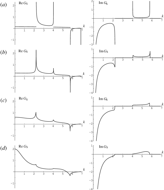
Figure 2: The real and imaginary parts of $G_{\rm S}(x,y;k)$ for the potential shown in figure 1, plotted as functions of real $k$, with various values of $h$. (a) $h=0$, (b) $h=0.2$, (c) $h=0.5$, (d) $h=1$. In all the graphs, $C=1$, $L=1$, $a=0.6$, $x=0.4$ and $y=0.1$. The graphs are shown here for the range of $k$ in the lowest two energy bands and the lowest two gaps. The bands are $0<k<k_{1}$ and $k_{2}<k<k_{3}$, and the gaps are $k_{1}<k<k_{2}$ and $k_{3}<k<k_{4}$, where $k_{1}\simeq 2.21$, $k_{2}\simeq 4.02$, $k_{3}\simeq 5.77$ and $k_{4}\simeq 6.88$. The imaginary part of $G_{\rm S}$ is identically zero in the gaps.

Figure 3: Same as figure 2, with larger values of $h$. (a) $h=2$, (b) $h=4$, (c) $h=\infty$. In (b), the real part of $G_{\rm S}(k)$ tends to a finite value ($\simeq 1000$) as $k\to 0$, although the graph is truncated at the top. The graph in (c) is the plot of (12.6). This graph diverges to infinity as $k\to 0$. The singularity at $k=\pi/a\simeq 5.24$ corresponds to an eigenvalue for the infinite square well potential. The peak around $k=\pi/a$ in the graphs of ${\rm Im}\,G_{\rm S}$ becomes a delta function as we let $h\to+\infty$.

The case $h=0$ corresponds to a purely periodic potential, which was studied section 11 of [2]. When $h=0$, the graphs are discontinuous at the edges of the energy bands (figure 2(a)). The graphs become continuous when $h\neq 0$, but singularities remain at the edges of the bands (figures 2 (b)–(d)). As $h$ is further increased, these singularities become less prominent in the graphs (figures 3(a) and (b)). In the extreme case $h=+\infty$, the potential is an infinite square well, for which the exact Green function is

$$G_{\rm S}(x,y;k)=\frac{\cos[k(x-a)]\cos(ky)}{k\sin(ka)}$$ (1.8ifmtabgbcfibcbghaf)

(see figure 3(c)). As $h$ becomes large, the Green function approaches (12.6) except at $k=n\pi/a$ ($n$ integer), where the right-hand side (12.6) has poles.

Now let us turn to the low-energy expansion. Since $V_{\Delta}\in L^{1}_{N}$ for any $N$, expansion (1.10) is valid for any $N$. We need to calculate the various quantities appearing in (8.9). The quantities involving only $V_{\rm p}$ (and not $V_{\Delta}$) have already been calculated in [2]. It is shown in section 11 of [2] that

$$L_{0}=\sqrt{(a+b\rme^{C})(a+b\rme^{-C})},\qquad V_{0}=\frac{1}{2}\log\frac{a+b\rme^{C}}{a+b\rme^{-C}},$$ (1.8ifmtabgbcfibcbghaga)

$$Q=\frac{1}{12}(a^{4}+6a^{2}b^{2}+b^{4})+\frac{ab}{3}(a^{2}+b^{2})\cosh C,$$ (1.8ifmtabgbcfibcbghagb)

$${}_{\rm p}[\hbox{$+$$-$}]_{x-L}^{x}=\frac{1}{2}(a^{2}+b^{2})+\rme^{-C}b(a-x)+\rme^{C}bx,$$ (1.8ifmtabgbcfibcbghagha)

$${}_{\rm p}[\hbox{$+$$-$$+$}]_{x-L}^{x}=\frac{a}{6}(a^{2}+3b^{2})+2bx(x-a)\sinh C+\frac{b}{6}(3a^{2}+b^{2})\rme^{C}.$$ (1.8ifmtabgbcfibcbghaghb)

The expressions for ${}_{\rm p}[\hbox{$-$$+$}]_{x-L}^{x}$ and ${}_{\rm p}[\hbox{$-$$+$$-$}]_{x-L}^{x}$ are obtained from (12.8a) and (12.8b), respectively, by changing the sign of $C$. Other integrals in (8.9) are also easy to calculate. For $0<z\leq x<a$, we can see that

$$[\hbox{$+$}]_{z}^{x}=\rme^{-h}(x-z),\qquad[\hbox{$+$$+$}]_{z}^{x}=\frac{\rme^{-2h}}{2}(x-z)^{2},\qquad[\hbox{$-$$+$}]_{z}^{x}=[\hbox{$+$$-$}]_{z}^{x}=\frac{1}{2}(x-z)^{2}.$$ (1.8ifmtabgbcfibcbghaghi)

The functions $\Delta^{\pm}$ defined by (5.16) are

$$\Delta^{\pm}(z)=\cases{\rme^{\mp h}-1&$(0<z<a)$\\ 0&(otherwise)}.$$ (1.8ifmtabgbcfibcbghaghj)

The integrals including $\Delta^{\pm}$ can be calculated, for example, as

$$\int_{-\infty}^{\infty}\rmd z\left[\rme^{V_{0}}\Delta^{-}(z)-\rme^{-V_{0}}\Delta^{+}(z)\right]=2a\left[\sinh(V_{0}+h)-\sinh V_{0}\right].$$ (1.8ifmtabgbcfibcbghaghk)

Substituting the above expressions in (8.9), we obtain

$$s_{0}=-\rme^{-(V_{0}+h)},\qquad s_{1}=\rme^{-(V_{0}+h)}a[\sinh(V_{0}+h)-\sinh V_{0}],$$

$$s_{2}=\frac{\rme^{-(2V_{0}+h)}}{L_{0}}\Biggl{[}\frac{a}{6}(a^{2}+3b^{2})+\frac{b}{6}(3a^{2}+b^{2})\rme^{C}+2bx(x-a)\rme^{-h}\sinh C-\frac{\rme^{V_{0}}}{8L_{0}}\left(L_{0}^{4}+4Q\right)\Biggr{]}$$

$$+\rme^{-2(V_{0}+h)}\left[x^{2}+(a-x)^{2}\right][\sinh(V_{0}+h)-\sinh V_{0}],$$

$$s_{3}=\frac{\rme^{-(2V_{0}+h)}}{2L_{0}}a\left(\rme^{-h}-1\right)\Biggl{[}\left(3\rme^{-V_{0}}+\rme^{V_{0}}\right)\frac{a}{6}(a^{2}+3b^{2})+\left(3\rme^{-V_{0}+C}+\rme^{V_{0}-C}\right)\frac{b}{6}(3a^{2}+b^{2})$$

$$-ba^{3}\left(\rme^{-h}+1\right)\rme^{-V_{0}}\sinh C-\frac{1}{2L_{0}}\left(L_{0}^{4}+4Q\right)\Biggr{]}$$

$$+\frac{\rme^{-(2V_{0}+h)}}{3}\left[x^{3}-(x-a)^{3}\right]\left(3\rme^{-V_{0}-2h}-\rme^{V_{0}}\right)\left[\sinh(V_{0}+h)-\sinh V_{0}\right],$$

with $L_{0}$, $V_{0}$ and $Q$ given by (12.7). (We have used $L_{0}=b\sinh C/\sinh V_{0}$.) Substituting (12.12) into (9.1), and then into (9.2), we obtain $g_{-1}$, $g_{0}$, $g_{1}$ and $g_{2}$. In particular,

$$g_{-1}=\frac{\rme^{V_{0}+h}}{2},\qquad g_{0}=\frac{1}{2}(x-y)+\frac{a}{2}\,\rme^{V_{0}+h}\left[\sinh(V_{0}+h)-\sinh V_{0}\right],$$ (1.8ifmtabgbcfibcbghaghm)

as can also be seen directly from (9.3). Thus, the expansion of the Green function is obtained to order $k^{2}$. This result is shown in figure 4 (the broken lines).

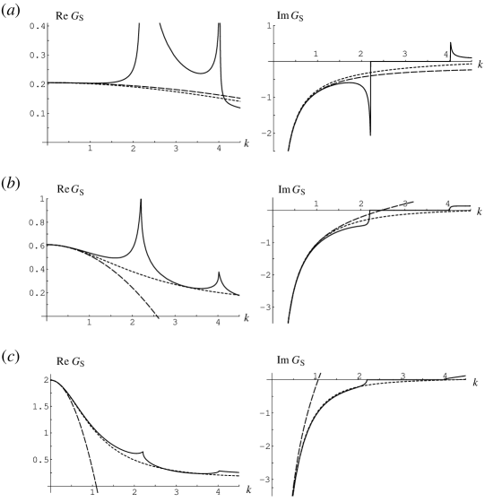
Figure 4: ${\rm Re}\,G_{\rm S}(x,y;k)$ and ${\rm Im}\,G_{\rm S}(x,y;k)$ plotted as functions of real $k$, for (a) $h=0.1$, (b) $h=0.5$ and (c) $h=1$. (All the other parameters are the same as in figures 2 and 3.) The solid lines show the exact Green function (close-up of figure 2). The broken lines show the result of the low-energy expansion up to order $k^{2}$. The dotted lines represent the approximation given by (12.21).

We can see from these graphs that this expansion is indeed correct.

For a potential like (12.1), there is a good approximation method which can be used for a wide range of $k$. Let us explain this approximation in connection with the power-series expansion of $\bar{R}_{r}$. From (5.7), (5.14), (5.15), (5.27) and (5.29), we have

$$\bar{r}_{0}=\tanh\frac{V_{0}-W}{2},\qquad\bar{r}_{1}=\frac{1}{\cosh^{2}\frac{W-V_{0}}{2}}\left[x\sinh(V_{0}+h)-\frac{a}{2}\sinh V_{0}\right],$$ (1.8ifmtabgbcfibcbghaghna)

$$\bar{r}_{2}=\frac{1}{\cosh^{3}\frac{W-V_{0}}{2}}\Biggl{\{}\left[x^{2}\sinh(V_{0}+h)-ax\sinh V_{0}\right]\cosh\frac{W+V_{0}+2h}{2}$$

$$-\frac{a}{12L_{0}}(a^{2}+3b^{2})\sinh\frac{W+V_{0}}{2}-\frac{b}{12L_{0}}(3a^{2}+b^{2})\sinh\frac{W+V_{0}-2C}{2}$$

$$+\frac{1}{16L_{0}^{2}}\left(L_{0}^{4}+4Q\right)\sinh\frac{W-V_{0}}{2}\Biggr{\}}.$$ (1.8ifmtabgbcfibcbghaghnb)

Recall that $R_{r}(x,-\infty;k)$ is obtained from $\bar{R}_{r}(x,-\infty;W;k)$ by setting $W=V(x)$. Since $V(x)=-h$ for $0<x<a$, the expansion of $R_{r}(x,-\infty;k)$ for $0<x<a$ is

$$R_{r}(x,-\infty;k)=r_{0}+\rmi kr_{1}+(\rmi k)^{2}r_{2}+\cdots,$$ (1.8ifmtabgbcfibcbghaghno)

where $r_{0}$ and $r_{1}$ are obtained by letting $W=-h$ in (12.14a) as

$$r_{0}=\tanh\frac{V_{0}+h}{2},\qquad r_{1}=2(x-\delta)r_{0},$$ (1.8ifmtabgbcfibcbghaghnp)

with $\delta$ defined by

$$\delta\equiv\frac{a\sinh V_{0}}{2\sinh(V_{0}+h)}.$$ (1.8ifmtabgbcfibcbghaghnq)

Setting $W=-h$ in (12.14b), we can see that

$$r_{2}=2(x-\delta)^{2}r_{0}+\cdots,$$ (1.8ifmtabgbcfibcbghaghnr)

where the terms represented by the dots behave like $\rme^{-h/2}$, and hence are negligible, when $h$ is large. In the same way, it can be shown that

$$r_{n}\simeq\frac{2^{n}}{n!}(x-\delta)^{n}r_{0}$$ (1.8ifmtabgbcfibcbghaghns)

for any $n$, when $h$ is large. Substituting (12.19) into (12.15) gives

$$R_{r}(x,-\infty;k)\simeq r_{0}\,\rme^{2\rmi k(x-\delta)}.$$ (1.8ifmtabgbcfibcbghaghnt)

From (12.3), (12.20) and the second equation of (12.4), we obtain the approximation

$$G_{\rm S}(x,y;k)\simeq\frac{\left[1+r_{0}\,\rme^{2\rmi k(a-x-\delta)}\right]\left[1+r_{0}\,\rme^{2\rmi k(y-\delta)}\right]\rme^{\rmi k(x-y)}}{2\rmi k\left[1-r_{0}^{2}\,\rme^{2\rmi k(a-2\delta)}\right]}.$$ (1.8ifmtabgbcfibcbghaghnu)

In fact, this approximation is equivalent to replacing the potential $V(z)$ by the effective square well potential

$$V_{\rm eff}(z)=\cases{-h&$(\delta<z<a-\delta)$\\ V_{0}&(otherwise)}.$$ (1.8ifmtabgbcfibcbghaghnv)

The result of this approximation is also plotted in figure 4 (the dotted lines). As we can see from figures 4(b) and 4(c), equation (12.21) gives a good approximation, when $h$ is not very small, for a wide range of $k$ except near the band edges. This approximation becomes better for larger $h$, so that the graphs shown in figures 3(a) and 3(b) can be very accurately approximated by (12.21).

Example 2.

Next, we study an example where the Schrödinger potential $V_{\rm S}$, rather than the Fokker-Planck potential $V$, is given. We consider $V_{\rm S}(x)=V^{\rm S}_{\rm p}(x)+V^{\rm S}_{\Delta}(x)$ with

$$V^{\rm S}_{\rm p}(x)=\cases{-E_{0}&$(0<x<a)$\\ C-E_{0}&$(a<x<L)$\\ },\qquad V^{\rm S}_{\rm p}(x+L)=V^{\rm S}_{\rm p}(x),$$ (1.8ifmtabgbcfibcbghaghnwa)

$$V^{\rm S}_{\Delta}(x)=\cases{h&$(0<x<a)$\\ 0&(otherwise)\\ }.$$ (1.8ifmtabgbcfibcbghaghnwb)

(See figure 5.) The periodic part $V_{\rm p}^{\rm S}$ is a Kronig-Penny potential [15]. We assume $h>0$ so that there are no bound states. The constant $E_{0}$ is determined by the condition that the energy at the bottom of the lowest band be zero. It is easy to see that $E_{0}$ is the smallest solution of the equation

$$\sqrt{C-E_{0}}\tanh\frac{b\sqrt{C-E_{0}}}{2}=\sqrt{E_{0}}\tan\frac{a\sqrt{E_{0}}}{2}.$$ (1.8ifmtabgbcfibcbghaghnwx)

The expansion of the Green function can be obtained by using the method explained in section 11. We define

$$p\equiv\sqrt{E_{0}},\qquad\!q\equiv\sqrt{C-E_{0}},\qquad\!s\equiv\sqrt{h-E_{0}},\qquad\!\xi\equiv\frac{q}{s}\tanh\frac{bq}{2}=\frac{p}{s}\tan\frac{ap}{2}.$$ (1.8ifmtabgbcfibcbghaghnwy)

The solution of (11.1) which remains bounded as $x\to+\infty$ is

$$\psi_{0}^{+}(x)=\cases{\cosh\,[s(x-a)]-\xi\sinh\,[s(x-a)]&$(0<x<a)$\\ {\rm sech}\,{\textstyle\frac{bq}{2}}\cosh\left[q\left(x-a-{\textstyle\frac{b}{2}}\right)\right]&$(a<x<L)$\\ \sec{\textstyle\frac{ap}{2}}\cos\left[p\left(x-L-{\textstyle\frac{a}{2}}\right)\right]&$(L<x<L+a)$\\ },$$ (1.8ifmtabgbcfibcbghaghnwz)

$$\psi_{0}^{+}(x+L)=\psi_{0}^{+}(x)\qquad(a<x).$$ (1.8ifmtabgbcfibcbghaghnwaa)

(We may multiply (12.26) by a positive constant factor, and this does not change the final result.) We do not write here the expression for $x<0$, but only remark that $\psi_{0}^{+}(x)\to+\infty$ as $x\to-\infty$. On account of the symmetry, $\psi_{0}^{-}$ is obtained from $\psi_{0}^{+}$ as

$$\psi_{0}^{-}(x)=\psi_{0}^{+}(a-x).$$ (1.8ifmtabgbcfibcbghaghnwab)

The graphs of $V^{+}(x)$ and $V^{-}(x)$ defined by (11.2) are shown in figure 5.

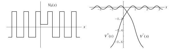
Figure 5: The Schrödinger potential $V_{\rm S}$ of example 2 (equations (12.23)) and the corresponding Fokker-Planck potentials $V^{\pm}$. The parameters used for these graphs are $C=1$, $L=1$, $a=0.6$ and $h=0.5$. From (12.24) we have $E_{0}\simeq 0.3952$.

Note that $V^{+}(x)\to-\infty$ as $x\to-\infty$ and $V^{-}(x)\to-\infty$ as $x\to+\infty$.

Let us calculate $g_{0}(x,y)$ and $g_{1}(x,y)$ for $0<y\leq x<a$. We have

$$\psi_{0}^{+}(x)=\cosh\,[s(x-a)]-\xi\sinh\,[s(x-a)],\qquad\psi_{0}^{-}(y)=\cosh sy+\xi\sinh sy.$$ (1.8ifmtabgbcfibcbghaghnwac)

The Wronskian can be calculated as

$$W[\psi_{0}^{+},\psi_{0}^{-}]=2\xi s\cosh sa+(1+\xi^{2})s\sinh sa.$$ (1.8ifmtabgbcfibcbghaghnwad)

Substituting (12.29) and (12.30) into (11.9) gives $g_{0}(x,y)$. To calculate $g_{1}$, we need to evaluate $V_{0}^{\pm}$. It is obvious that $V_{0}^{+}=V_{0}^{-}$. By definition,

$$\rme^{-V_{0}^{+}}=\rme^{-V_{0}^{-}}=\sqrt{M/P},\qquad P=\int_{x}^{x+L}\rme^{V_{\rm p}^{+}(z)}\,\rmd z,\qquad M=\int_{x}^{x+L}\rme^{-V_{\rm p}^{+}(z)}\,\rmd z.$$ (1.8ifmtabgbcfibcbghaghnwae)

Since $V^{+}(z)=V_{\rm p}^{+}(z)$ for $z>a$, we can calculate, by using (12.26),

$$P=\int_{a}^{L+a}\!\!\!\frac{1}{[\psi_{0}^{+}(z)]^{2}}\,\rmd z=\frac{1}{q}\sinh bq+\frac{1}{p}\sin ap,$$ (1.8ifmtabgbcfibcbghaghnwafa)

$$M=\int_{a}^{L+a}[\psi_{0}^{+}(z)]^{2}\,\rmd z=\frac{b}{2}{\rm sech}^{2}\,\frac{bq}{2}+\frac{a}{2}\sec^{2}\frac{ap}{2}+\frac{1}{q}\tanh\frac{bq}{2}+\frac{1}{p}\tan\frac{ap}{2}.$$ (1.8ifmtabgbcfibcbghaghnwafb)

For $0<y\leq x<a$, we can also calculate the integrals

$$\int_{y}^{x}\rme^{V^{+}(z)}\,\rmd z=\frac{\sinh[s(x-a)]}{s\psi_{0}^{+}(x)}-\frac{\sinh[s(y-a)]}{s\psi_{0}^{+}(y)},\qquad\int_{y}^{x}\rme^{V^{-}(z)}\,\rmd z=\frac{\sinh sx}{s\psi_{0}^{-}(x)}-\frac{\sinh sy}{s\psi_{0}^{-}(y)}.$$

Substituting the above expressions into (11.8b), we obtain

$$g_{1}(x,y)=-\frac{1}{2}\sqrt{\frac{(b/2){\rm sech}^{2}\,\frac{bq}{2}+(a/2)\sec^{2}\frac{ap}{2}+(1/q)\tanh\frac{bq}{2}+(1/p)\tan\frac{ap}{2}}{(1/q)\sinh bq+(1/p)\sin ap}}$$

$$\times\Biggl{\{}\frac{\sinh[s(x-a)]}{s\psi_{0}^{+}(x)}-\frac{\sinh[s(y-a)]}{s\psi_{0}^{+}(y)}+\frac{\sinh sx}{s\psi_{0}^{-}(x)}-\frac{\sinh sy}{s\psi_{0}^{-}(y)}$$

$$\quad\ \ +\frac{1}{W[\psi_{0}^{+},\psi_{0}^{-}]}\left(\frac{\psi_{0}^{+}(x)}{\psi_{0}^{-}(x)}+\frac{\psi_{0}^{-}(x)}{\psi_{0}^{+}(x)}+\frac{\psi_{0}^{+}(y)}{\psi_{0}^{-}(y)}+\frac{\psi_{0}^{-}(y)}{\psi_{0}^{+}(y)}\right)\Biggr{\}}\frac{\psi_{0}^{+}(x)\psi_{0}^{-}(y)}{W[\psi_{0}^{+},\psi_{0}^{-}]},$$

where $\psi_{0}^{+}(x)$, $\psi_{0}^{-}(y)$ and $W[\psi_{0}^{+},\psi_{0}^{-}]$ are given by (12.29) and (12.30).

The exact Green function for this potential is shown in appendix C (equation (C.2)). Comparing with this exact expression, we can check that (12.34) gives the correct first-order coefficient of the expansion (see figure 6).

Figure 6: The real and imaginary parts of the exact $G_{\rm S}(x,y;k)$ for example 2 (equation (C.2) of appendix C), plotted as functions of real $k$, with $x=0.4$ and $y=0.1$. All other parameters are the same as in figure 5. The range of $k$ shown in these graphs is entirely included in the lowest energy band. (The edge of the band is at $k\simeq 3.094$.) The broken line is the line with slope $g_{1}\simeq-21.85$, which is the value given by (12.34). (The value of $g_{0}$ obtained from (11.9) is $g_{0}\simeq-3.28$.)

Appendix A Derivation of (7.8)

We will show that

$$\lim_{k\to 0}\int_{-\infty}^{x}\bar{Q}(x,z;W;k)\,g_{\rm p}(z,\bar{\omega}(x,z;W;k))\,\rmd z$$

$$=\lim_{k\to 0}\int_{-\infty}^{x}\bar{Q}_{\rm p}(x,z;W;k)\,g_{\rm p}(z,\bar{\omega}_{\rm p}(x,z;W;k))\,\rmd z,$$ (1.8ifmtabgbcfibcbghaghnwafa)

where $g_{\rm p}(x,W)$ is a function satisfying (4.10). We assume that $g_{\rm p}(x,W)$ is analytic with respect to $W$ on the real axis.

Let $\bar{\alpha}$ and $\bar{\beta}$ be defined by

$$\left(\begin{array}[]{cc}\bar{\alpha}(x,z;W;k)&\bar{\beta}(x,z;W;-k)\\ \bar{\beta}(x,z;W;k)&\bar{\alpha}(x,z;W;-k)\\ \end{array}\right)$$ (1.8ifmtabgbcfibcbghaghnwafd)

$$\qquad\ \ \equiv\left(\begin{array}[]{cc}\cosh\frac{W-V(x)}{2}&-\sinh\frac{W-V(x)}{2}\\ -\sinh\frac{W-V(x)}{2}&\cosh\frac{W-V(x)}{2}\\ \end{array}\right)\left(\begin{array}[]{cc}\alpha(x,z;k)&\beta(x,z;-k)\\ \beta(x,z;k)&\alpha(x,z;-k)\\ \end{array}\right).$$ (1.8ifmtabgbcfibcbghaghnwafi)

Then, $\bar{\tau}$, $\bar{R}_{r}$ and $\bar{R}_{l}$ are expressed in terms of $\bar{\alpha}$ and $\bar{\beta}$ as

$$\bar{\tau}(x,z;W;k)=\frac{1}{\bar{\alpha}(x,z;W;k)},\qquad\bar{R}_{r}(x,z;W;k)=\frac{\bar{\beta}(x,z;W;k)}{\bar{\alpha}(x,z;W;k)},$$

$$\bar{R}_{l}(x,z;W;k)=-\frac{\bar{\beta}(x,z;W;-k)}{\bar{\alpha}(x,z;W;k)}.$$ (1.8ifmtabgbcfibcbghaghnwafj)

Substituting (A.3) into (7.2) and (3.6), we can write $\bar{Q}$ and $\bar{\omega}$ as

$$\bar{Q}(x,z;W;k)=\frac{1}{[\bar{\alpha}(x,z;W;k)+\bar{\beta}(x,z;W;-k)][\bar{\alpha}(x,z;W;k)-\bar{\beta}(x,z;W;-k)]},$$

$$\bar{\omega}(x,z;W;k)=V(z)+\log\frac{\bar{\alpha}(x,z;W;k)-\bar{\beta}(x,z;W;-k)}{\bar{\alpha}(x,z;W;k)+\bar{\beta}(x,z;W;-k)}.$$ (1.8ifmtabgbcfibcbghaghnwafk)

Let $\bar{\alpha}_{\rm P}$ and $\bar{\beta}_{\rm p}$ be the quantities obtained from $\bar{\alpha}$ and $\bar{\beta}$, respectively, by replacing $V$ with $V_{\rm p}$. Then, just like (A.3) and (A.4), we have

$$\bar{\tau}^{\rm p}(x,z;W;k)=\frac{1}{\bar{\alpha}_{\rm P}(x,z;W;k)},\qquad\bar{R}_{r}^{\rm p}(x,z;W;k)=\frac{\bar{\beta}_{\rm P}(x,z;W;k)}{\bar{\alpha}_{\rm P}(x,z;W;k)},$$

$$\bar{R}_{l}^{\rm p}(x,z;W;k)=-\frac{\bar{\beta}_{\rm P}(x,z;W;-k)}{\bar{\alpha}_{\rm P}(x,z;W;k)}$$ (1.8ifmtabgbcfibcbghaghnwafl)

and

$$\bar{Q}_{\rm p}(x,z;W;k)=\frac{1}{[\bar{\alpha}_{\rm p}(x,z;W;k)+\bar{\beta}_{\rm p}(x,z;W;-k)][\bar{\alpha}_{\rm p}(x,z;W;k)-\bar{\beta}_{\rm p}(x,z;W;-k)]},$$

$$\bar{\omega}_{\rm p}(x,z;W;k)=V_{\rm p}(z)+\log\frac{\bar{\alpha}_{\rm p}(x,z;W;k)-\bar{\beta}_{\rm p}(x,z;W;-k)}{\bar{\alpha}_{\rm p}(x,z;W;k)+\bar{\beta}_{\rm p}(x,z;W;-k)}.$$ (1.8ifmtabgbcfibcbghaghnwafm)

Before carrying out the calculation, let us note that the following equations hold for an arbitrary finite number $x_{0}\leq x$:

$$\lim_{k\to 0}\int_{-\infty}^{x}\bar{Q}_{\rm p}(x,z;W;k)g_{\rm p}(z,\bar{\omega}_{\rm p}(x,z;W;k))\,\rmd z$$

$$=\lim_{k\to 0}\int_{-\infty}^{x_{0}}\bar{Q}_{\rm p}(x_{0},z;W;k)g_{\rm p}(z,\bar{\omega}_{\rm p}(x_{0},z;W;k))\,\rmd z+\int_{x_{0}}^{x}g_{\rm p}(z,W)\,\rmd z,$$

$$\lim_{k\to 0}\int_{-\infty}^{x}\bar{Q}(x,z;W;k)g_{\rm p}(z,\bar{\omega}(x,z;W;k))\,\rmd z$$

$$=\lim_{k\to 0}\int_{-\infty}^{x_{0}}\bar{Q}(x_{0},z;W;k)g_{\rm p}(z,\bar{\omega}(x_{0},z;W;k))\,\rmd z+\int_{x_{0}}^{x}g_{\rm p}(z,W)\,\rmd z.$$

Equation (A.7) is derived from the two equations

$$\lim_{k\to 0}\int_{x_{0}}^{x}\bar{Q}_{\rm p}(x,z;W;k)g_{\rm p}(z,\bar{\omega}_{\rm p}(x,z;W;k))\,\rmd z=\int_{x_{0}}^{x}g_{\rm p}(z,W)\,\rmd z$$ (1.8ifmtabgbcfibcbghaghnwafp)

and

$$\lim_{k\to 0}\int_{-\infty}^{x_{0}}\bar{Q}_{\rm p}(x,z;W;k)g_{\rm p}(z,\bar{\omega}_{\rm p}(x,z;W;k))\,\rmd z$$

$$=\lim_{k\to 0}\int_{-\infty}^{x_{0}}\bar{Q}_{\rm p}(x_{0},z;W;k)g_{\rm p}(z,\bar{\omega}_{\rm p}(x_{0},z;W;k))\,\rmd z.$$ (1.8ifmtabgbcfibcbghaghnwafq)

The proof of (A.9) is easy. Since the limit and the integral on the left-hand side are interchangeable, we can use (7.7) to obtain (A.9). The outline of the proof of (A.10) is as follows. From $U(x,x_{0};k)U(x_{0},z;k)=U(x,z;k)$ and (A.2), we have

$$\bar{\alpha}_{\rm p}(x,z;W;k)\pm\bar{\beta}_{\rm p}(x,z;W;-k)=\bar{\alpha}_{\rm p}(x,x_{0};W;k)[\alpha_{\rm p}(x_{0},z;k)\pm\beta_{\rm p}(x_{0},z;-k)]$$

$$+\bar{\beta}_{\rm p}(x,x_{0};W;-k)[\beta_{\rm p}(x_{0},z;k)\pm\alpha_{\rm p}(x_{0},z;-k)].$$ (1.8ifmtabgbcfibcbghaghnwafr)

From (2.1) and (A.2), we can easily see that

$$\bar{\alpha}_{\rm p}(x,x_{0};W;k)=\cosh\frac{W-V_{\rm p}(x_{0})}{2}+C_{1}(k),\qquad C_{1}(k)=O(k)\ \ \hbox{as}\ \ k\to 0,$$

$$\bar{\beta}_{\rm p}(x,x_{0};W;-k)=-\sinh\frac{W-V_{\rm p}(x_{0})}{2}+C_{2}(k),\qquad C_{2}(k)=O(k)\ \ \hbox{as}\ \ k\to 0.$$ (1.8ifmtabgbcfibcbghaghnwafs)

We substitute (A.11) and (A.12) into (A.6), and calculate the left-hand side of (A.10) by using the method described in section 5 of [2]. Then we find that the contributions from $C_{1}(k)$ and $C_{2}(k)$ vanish in the limit $k\to 0$. It is easy to show that $\bar{Q}_{\rm p}(x,z)$ and $\bar{\omega}_{\rm p}(x,z)$ become $\bar{Q}_{\rm p}(x_{0},z)$ and $\bar{\omega}_{\rm p}(x_{0},z)$, respectively, when $C_{1}(k)$ and $C_{2}(k)$ of (A.12) are set to be zero. Hence we obtain (A.10). Adding both sides of (A.9) and (A.10) yields (A.7). Equation (A.8) can be proved in essentially the same way. Using (A.7) and (A.8), equation (A.1) is reduced to

$$\lim_{k\to 0}\int_{-\infty}^{x_{0}}\bar{Q}(x_{0},z;W;k)\,g_{\rm p}(z,\bar{\omega}(x_{0},z;W;k))\,\rmd z$$

$$=\lim_{k\to 0}\int_{-\infty}^{x_{0}}\bar{Q}_{\rm p}(x_{0},z;W;k)\,g_{\rm p}(z,\bar{\omega}_{\rm p}(x_{0},z;W;k))\,\rmd z,$$ (1.8ifmtabgbcfibcbghaghnwaft)

where $x_{0}$ is arbitrary. The meaning of the equivalence between (A.1) and (A.13) is easy to understand. Since $\lim_{k\to 0}\bar{Q}=\lim_{k\to 0}\bar{Q}_{\rm p}$ and $\lim_{k\to 0}\bar{\omega}=\lim_{k\to 0}\bar{\omega}_{\rm p}$, the difference between the left-hand and right-hand sides of (A.1) in the limit $k\to 0$ is determined only by the behavior at $z\to-\infty$. So, in (A.1), we can arbitrarily change the value of $x$ as long as it remains finite. Also note that equations (A.7) and (A.8), respectively, correspond to

$$(\mathcal{A}_{\rm p}^{-1}g_{\rm p})(x,W)=(\mathcal{A}_{\rm p}^{-1}g_{\rm p})(x_{0},W)+\int_{x_{0}}^{x}g_{\rm p}(z,W)\,\rmd z,$$

$$(\mathcal{A}^{-1}g_{\rm p})(x,W)=(\mathcal{A}^{-1}g_{\rm p})(x_{0},W)+\int_{x_{0}}^{x}g_{\rm p}(z,W)\,\rmd z$$ (1.8ifmtabgbcfibcbghaghnwafu)

(see equation (5.34) of [2]).

Since (A.1) and (A.13) are equivalent, we will deal with (A.13) instead of (A.1). By taking $-x_{0}$ to be sufficiently large, we can make $|V_{\Delta}(z)|$ to be arbitrarily small for $z\leq x_{0}$.

Let us review how to calculate the right-hand side of (A.13). (See [2] for details.) We split the integral into unit periods as

$$\int_{-\infty}^{x_{0}}\bar{Q}_{\rm p}(x_{0},z;W;k)\,g_{\rm p}(z,\bar{\omega}_{\rm p}(x_{0},z;W;k))\,\rmd z=\sum_{n=0}^{\infty}A_{n}(k),$$ (1.8ifmtabgbcfibcbghaghnwafv)

$$A_{n}(k)\equiv\int_{x_{0}-(n+1)L}^{x_{0}-nL}\bar{Q}_{\rm p}(x_{0},z;W;k)\,g_{\rm p}(z,\bar{\omega}_{\rm p}(x_{0},z;W;k))\,\rmd z.$$ (1.8ifmtabgbcfibcbghaghnwafw)

Let $\lambda$ and $\lambda^{-1}$ be the eigenvalues of the matrix

$$\left(\begin{array}[]{cc}\alpha_{\rm p}(x,x-L;k)&\beta_{\rm p}(x,x-L;-k)\\ \beta_{\rm p}(x,x-L;k)&\alpha_{\rm p}(x,x-L;-k)\\ \end{array}\right)$$ (1.8ifmtabgbcfibcbghaghnwafx)

such that $|\lambda|\geq 1$ for ${\rm Im}\,k\geq 0$. Namely,

$$\lambda\equiv Y-\rmi\sqrt{1-Y^{2}},\qquad Y\equiv\frac{1}{2}\left[\alpha_{\rm p}(x,x-L;k)+\alpha_{\rm p}(x,x-L;-k)\right].$$ (1.8ifmtabgbcfibcbghaghnwafy)

We define

$$\gamma\equiv\lambda^{-2}.$$ (1.8ifmtabgbcfibcbghaghnwafz)

It turns out that $A_{n}(k)$ depends on $n$ only through $\gamma^{n}$. Moreover, it also turns out that $A_{n}(k)$ has the form

$$A_{n}(k)=k\gamma^{n}C(\gamma^{n},k),$$ (1.8ifmtabgbcfibcbghaghnwafaa)

where $C(\gamma^{n},k)$ is an analytic function of $k$ and $\gamma^{n}$ on the real axis. We have $|\gamma|<1$ for ${\rm Im}\,k>0$ and $|\gamma|=1$ for ${\rm Im}\,k=0$. The behavior of $\gamma$ for small $k$ is

$$\gamma=1+2\rmi L_{0}k+O(k^{2})\qquad\hbox{as}\quad k\to 0.$$ (1.8ifmtabgbcfibcbghaghnwafab)

Since the approach of $\gamma^{n}$ to 1 is not uniform in $n$, we cannot change the order of the limit and the sum as

$$\lim_{k\to 0}\sum_{n=0}^{\infty}k\gamma^{n}C(\gamma^{n},k)=\sum_{n=0}^{\infty}\lim_{k\to 0}k\gamma^{n}C(\gamma^{n},k)=0.$$ (1.8ifmtabgbcfibcbghaghnwafac)

However, if we treat $k$ and $\gamma^{n}$ separately, we can let $k\to 0$ inside the sum as

$$\lim_{k\to 0}k\sum_{n=0}^{\infty}\gamma^{n}C(\gamma^{n},k)=\lim_{k\to 0}k\sum_{n=0}^{\infty}\gamma^{n}C(\gamma^{n},0).$$ (1.8ifmtabgbcfibcbghaghnwafad)

As a result, we have

$$\lim_{k\to 0}\,k\sum_{n=0}^{\infty}\gamma^{n}C(\gamma^{n},k)=\frac{\rmi}{2L_{0}}\int_{0}^{1}C(x,0)\,\rmd x.$$ (1.8ifmtabgbcfibcbghaghnwafae)

This equation can be intuitively understood as follows. From (A.21), we can see that $\gamma^{n}$ behaves like $\exp(2\rmi L_{0}kn)$ when $k$ is small. Therefore,

$$\lim_{k\to 0}\,k\sum_{n=0}^{\infty}\gamma^{n}C(\gamma^{n},k)=\lim_{k=0}\,k\int_{0}^{\infty}\rme^{2\rmi L_{0}k\nu}C(\rme^{2\rmi L_{0}k\nu},k)\,\rmd\nu=\frac{\rmi}{2L_{0}}\lim_{k\to 0}\int_{0}^{1}C(x,k)\,\rmd x.$$

In (A.25), we changed the sum over discrete $n$ to an integral over continuous $\nu$, and then changed the variable of integration to $x\equiv\rme^{2\rmi L_{0}k\nu}$. Here, let us comment about the meaning of $\lim_{k\to 0}$. The limit $k\to 0$ can be taken in any way in the closed upper half plane (${\rm Im}\,k\geq 0$), but we need to be careful when the limit is taken along the real axis (${\rm Im}\,k=0$). Recall that we have defined the Green function for ${\rm Im}\,k=0$ as $G_{\rm S}(x,y;k)\equiv\lim_{\epsilon\downarrow 0}G_{\rm S}(x,y;k+\rm i\epsilon)$. So when we write an expression like $\lim_{k\to 0}a(k)$, it is to be understood as $\lim_{k\to 0}\lim_{\epsilon\downarrow 0}a(k+\rmi\epsilon)$ for real $k$. Therefore, in (A.25), $x\to 0$ as $\nu\to\infty$ inside the limit sign. The limit and the integral in the last expression of (A.25) can be interchanged, since $|C(x,k)|$ is uniformly bounded when $|k|$ is sufficiently small. Hence we have (A.24).

The left-hand side of (A.13) is calculated in almost the same way. The only difference is that the quantity corresponding to $A_{n}(k)$ contains a part which depends explicitly on $n$, in addition to the part which depends on $n$ through $\gamma^{n}$. If we write

$$\int_{-\infty}^{x_{0}}\bar{Q}(x_{0},z;W;k)\,g_{\rm p}(z,\bar{\omega}(x_{0},z;W;k))\,\rmd z\equiv\sum_{n=0}^{\infty}A^{\prime}_{n}(k),$$ (1.8ifmtabgbcfibcbghaghnwafag)

then $A^{\prime}_{n}(k)$ has the form

$$A^{\prime}_{n}(k)=k\gamma^{n}C(\gamma^{n},k)+D_{n}(\gamma^{n},k).$$ (1.8ifmtabgbcfibcbghaghnwafah)

As we will see, $D_{n}$ decreases like $V_{\Delta}(x_{0}-nL)$ as $n\to\infty$. If $V_{\Delta}\in F^{(-)}_{0}$, there exists a $k$-independent (and $\gamma^{n}$-independent) sequence $\{E_{n}\}$ such that $|D_{n}(\gamma^{n},k)|<E_{n}$ and $\sum_{n=0}^{\infty}E_{n}<\infty$. Then, we have

$$\lim_{k\to 0}\sum_{n=0}^{\infty}D_{n}(\gamma^{n},k)=\sum_{n=0}^{\infty}D_{n}(1,0).$$ (1.8ifmtabgbcfibcbghaghnwafai)

We will show that the right-hand side of (A.28) is zero.

Now let us explicitly calculate the difference between the right-hand and left-hand sides of (A.13). Since $|V_{\Delta}|$ can be made as small as we like by taking large $|x_{0}|$, we consider only the terms of first order in $V_{\Delta}$. We can write

$$\int_{-\infty}^{x_{0}}\bar{Q}(x_{0},z;W;k)g_{\rm p}(z,\bar{\omega}(x_{0},z;W;k))\,\rmd z$$

$$\quad-\int_{-\infty}^{x_{0}}\bar{Q}_{\rm p}(x_{0},z;W;k)g_{\rm p}(z,\bar{\omega}_{\rm p}(x_{0},z;W;k))\,\rmd z$$

$$=\int_{-\infty}^{x_{0}}\bar{Q}_{\Delta}(x_{0},z;W;k)g_{\rm p}(z,\bar{\omega}_{\rm p}(x_{0},z;W;k))\,\rmd z$$

$$\quad+\int_{-\infty}^{x_{0}}\bar{Q}_{\rm p}(x_{0},z;W;k)\bar{\omega}_{\Delta}(x_{0},z;W;k)g^{\prime}_{\rm p}(z,\bar{\omega}_{\rm p}(x_{0},z;W;k))\,\rmd z,$$ (1.8ifmtabgbcfibcbghaghnwafaj)

where

$$\bar{Q}_{\Delta}\equiv\bar{Q}-\bar{Q}_{\rm p},\qquad\bar{\omega}_{\Delta}\equiv\bar{\omega}-\bar{\omega}_{\rm p},\qquad g^{\prime}_{\rm p}(z,W)\equiv\frac{\partial}{\partial W}g_{\rm p}(z,W).$$ (1.8ifmtabgbcfibcbghaghnwafak)

We define

$$\zeta_{\rm p}(z)\equiv\bar{\alpha}_{\rm p}(x_{0},z;W;k)+\bar{\beta}_{\rm p}(x_{0},z;W;-k),$$

$$\eta_{\rm p}(z)\equiv\bar{\alpha}_{\rm p}(x_{0},z;W;k)-\bar{\beta}_{\rm p}(x_{0},z;W;-k)$$ (1.8ifmtabgbcfibcbghaghnwafal)

and

$$\zeta(z)\equiv\bar{\alpha}(x_{0},z;W;k)+\bar{\beta}(x_{0},z;W;-k),$$

$$\eta(z)\equiv\bar{\alpha}(x_{0},z;W;k)-\bar{\beta}(x_{0},z;W;-k).$$ (1.8ifmtabgbcfibcbghaghnwafam)

Then, as can be seen from (A.4) and (A.6),

$$\bar{Q}_{\rm P}(x_{0},z;W;k)=\frac{1}{\zeta_{\rm P}(z)\eta_{\rm P(}z)},\qquad \bar{\omega}_{\rm P}(x_{0},z;W;k)=V_{\rm P}(z)+\log\frac{\eta_{\rm P}(z)}{\zeta_{\rm P(}z)},$$ (1.8ifmtabgbcfibcbghaghnwafan)

$$\bar{Q}(x_{0},z;W;k)=\frac{1}{\zeta(z)\eta(z)},\qquad \bar{\omega}(x_{0},z;W;k)=V(z)+\log\frac{\eta(z)}{\zeta(z)}.$$ (1.8ifmtabgbcfibcbghaghnwafao)

We can express $\bar{Q}_{\Delta}$ and $\bar{\omega}_{\Delta}$ as

$$\bar{Q}_{\Delta}=-\frac{1}{\zeta_{\rm p}\eta_{\rm p}}\left(\frac{\zeta_{\Delta}}{\zeta_{\rm p}}+\frac{\eta_{\Delta}}{\eta_{\rm p}}\right),\qquad\bar{\omega}_{\Delta}=V_{\Delta}-\frac{\zeta_{\Delta}}{\zeta_{\rm p}}+\frac{\eta_{\Delta}}{\eta_{\rm p}},$$ (1.8ifmtabgbcfibcbghaghnwafap)

where

$$\zeta_{\Delta}(z)\equiv\zeta(z)-\zeta_{\rm p}(z),\qquad\eta_{\Delta}(z)\equiv\eta(z)-\eta_{\rm p}(z).$$ (1.8ifmtabgbcfibcbghaghnwafaq)

Substituting (A.35) into (A.29) gives

$$\int_{-\infty}^{x_{0}}\bar{Q}(x_{0},z;W;k)g_{\rm p}(z,\bar{\omega}(x_{0},z;W;k))\,\rmd z$$

$$\quad-\int_{-\infty}^{x_{0}}\bar{Q}_{\rm p}(x_{0},z;W;k)g_{\rm p}(z,\bar{\omega}_{\rm p}(x_{0},z;W;k))\,\rmd z$$

$$=\int_{-\infty}^{x_{0}}\frac{-\zeta_{\Delta}(z)}{\zeta_{\rm p}^{2}(z)\eta_{\rm p}(z)}\left[g_{\rm p}(z,\bar{\omega}_{\rm p})+g^{\prime}_{\rm p}(z,\bar{\omega}_{\rm p})\right]\rmd z$$

$$\quad+\int_{-\infty}^{x_{0}}\frac{-\eta_{\Delta}(z)}{\zeta_{\rm p}(z)\eta_{\rm p}^{2}(z)}\left[g_{\rm p}(z,\bar{\omega}_{\rm p})-g^{\prime}_{\rm p}(z,\bar{\omega}_{\rm p})\right]\rmd z$$

$$\quad+\int_{-\infty}^{x_{0}}\frac{V_{\Delta}(z)}{\zeta_{\rm p}(z)\eta_{\rm p}(z)}\,g^{\prime}_{\rm p}(z,\bar{\omega}_{\rm p})\,\rmd z.$$ (1.8ifmtabgbcfibcbghaghnwafar)

As in (A.15) and (A.16), we calculate each integral for $x_{0}-nL\geq z\geq x_{0}-(n+1)L$, and then take the sum over $n$. So we need the expressions of $\zeta_{\rm p}(z)$, $\eta_{\rm p}(z)$, $\zeta_{\Delta}(z)$ and $\eta_{\Delta}(z)$ for $x_{0}-nL\geq z\geq x_{0}-(n+1)L$. It is shown in [2] that

$$\zeta_{\rm p}(z)=\rme^{u(z)}(\cosh w\,\lambda^{n}-\sinh w\,\lambda^{-n})-\rmi k\rme^{v(z)}(\cosh w\,\lambda^{n}+\sinh w\,\lambda^{-n})\,{}_{\rm p}[\hbox{$-$}]_{z}^{x_{0}-nL}$$

$$+\rme^{u}C(\lambda)k+o(k),$$

$$\eta_{\rm p}(z)=\rme^{-u(z)}(\cosh w\,\lambda^{n}+\sinh w\,\lambda^{-n})-\rmi k\rme^{-v(z)}(\cosh w\,\lambda^{n}-\sinh w\,\lambda^{-n})\,{}_{\rm p}[\hbox{$+$}]_{z}^{x_{0}-nL}$$

$$+\rme^{-u(z)}C(\lambda)k+o(k),$$ (1.8ifmtabgbcfibcbghaghnwafas)

where $w$, $u$ and $v$ are defined by

$$w\equiv\frac{W-V_{0}}{2},\qquad v(z)\equiv\frac{V_{\rm p}(z)+V_{0}}{2},\qquad u(z)\equiv\frac{V_{\rm p}(z)-V_{0}}{2}.$$ (1.8ifmtabgbcfibcbghaghnwafat)

In (A.38), and in equations (A.40), we let $C(\lambda)$ stand for a $z$-independent function of $\lambda$ which is not necessarily the same everywhere. The expressions for $\zeta_{\Delta}(z)$ and $\eta_{\Delta}(z)$ can be obtained, after some calculation, as

$$\zeta_{\Delta}(z)=\rme^{u(z)}\sum_{m=0}^{n-1}B_{m}(\sinh w\,\lambda^{n-2m-1}-\cosh w\,\lambda^{-n+2m+1})$$

$$-\rmi k\rme^{v(z)}\,{}_{\rm p}[\hbox{$-$}]_{z}^{x_{0}-nL}\sum_{m=0}^{n-1}B_{m}(\sinh w\,\lambda^{n-2m-1}+\cosh w\,\lambda^{-n+2m+1})$$

$$-\frac{1}{2}V_{\Delta}(x_{0})\,\rme^{u(z)}(\sinh w\,\lambda^{n}-\cosh w\,\lambda^{-n})$$

$$+\frac{\rmi k}{2}V_{\Delta}(x_{0})\,\rme^{v(z)}\,{}_{\rm p}[\hbox{$-$}]_{z}^{x_{0}-nL}\,(\sinh w\,\lambda^{n}+\cosh w\,\lambda^{-n})$$

$$+\frac{1}{2}\left[V_{\Delta}(z)-V_{\Delta}(x_{0}-nL)\right]\,\rme^{u(z)}(\cosh w\,\lambda^{n}-\sinh w\,\lambda^{-n})$$

$$+\rme^{u(z)}C(\lambda)k+o(k),$$

$$\eta_{\Delta}(z)=\rme^{-u(z)}\sum_{m=0}^{n-1}B_{m}(\sinh w\,\lambda^{n-2m-1}+\cosh w\,\lambda^{-n+2m+1})$$

$$-\rmi k\rme^{-v(z)}\,{}_{\rm p}[\hbox{$+$}]_{z}^{x_{0}-nL}\sum_{m=0}^{n-1}B_{m}(\sinh w\,\lambda^{n-2m-1}-\cosh w\,\lambda^{-n+2m+1})$$

$$-\frac{1}{2}V_{\Delta}(x_{0})\,\rme^{-u(z)}(\sinh w\,\lambda^{n}+\cosh w\,\lambda^{-n})$$

$$+\frac{\rmi k}{2}V_{\Delta}(x_{0})\,\rme^{-v(z)}\,{}_{\rm p}[\hbox{$+$}]_{z}^{x_{0}-nL}\,(\sinh w\,\lambda^{n}-\cosh w\,\lambda^{-n})$$

$$-\frac{1}{2}\left[V_{\Delta}(z)-V_{\Delta}(x_{0}-nL)\right]\,\rme^{-u(z)}(\cosh w\,\lambda^{n}+\sinh w\,\lambda^{-n})$$

$$+\rme^{-u(z)}C(\lambda)k+o(k),$$ (1.8ifmtabgbcfibcbghaghnwafau)

where

$$B_{m}\equiv\frac{1}{2}\left[V_{\Delta}(x_{0}-mL)-V_{\Delta}(x_{0}-(m+1)L)\right].$$ (1.8ifmtabgbcfibcbghaghnwafav)

Let us consider the first term on the right-hand side of (A.37). We divide the integral into unit periods and write

$$\int_{-\infty}^{x_{0}}\frac{-\zeta_{\Delta}(z)}{\zeta_{\rm p}^{2}(z)\eta_{\rm p}(z)}\,g_{\rm p}(z,\bar{\omega}_{\rm p})\,\rmd z=\sum_{n=0}^{\infty}\int_{x_{0}-(n+1)L}^{x_{0}-nL}\frac{-\zeta_{\Delta}(z)}{\zeta_{\rm p}^{2}(z)\eta_{\rm p}(z)}\,g_{\rm p}(z,\bar{\omega}_{\rm p})\,\rmd z$$

$$=\sum_{n=0}^{\infty}\int_{x_{0}-(n+1)L}^{x_{0}-nL}a(z,k)\,b(z,k)\,d(z,k)\,\rmd z,$$ (1.8ifmtabgbcfibcbghaghnwafaw)

where we have defined

$$a(z,k)\equiv\frac{\rme^{u(z)}\lambda^{n}\cosh w}{\zeta_{\rm p}^{2}(z)\eta_{\rm p}(z)},\qquad b(z,k)\equiv g_{\rm p}(z,\bar{\omega}_{\rm p}),\qquad d(z,k)\equiv\frac{-\zeta_{\Delta}(z)}{\rme^{u(z)}\lambda^{n}\cosh w}.$$ (1.8ifmtabgbcfibcbghaghnwafax)

From (A.38) and (A.40), we obtain the expressions for $a(z,k)$, $b(z,k)$ and $d(z,k)$ as

$$a(z,k)=a_{0}(\gamma^{n})+ka_{1}(z,\gamma^{n})+o(k),$$

$$b(z,k)=b_{0}(z)+kb_{1}(z,\gamma^{n})+o(k),$$

$$d(z,k)=d_{0}(z,\gamma)+kd_{1}(z,\gamma)+o(k),$$ (1.8ifmtabgbcfibcbghaghnwafay)

$$a_{0}(\gamma^{n})=\frac{\gamma^{n}}{(\cosh w)^{2}(1-c_{0}\gamma^{n})(1+c_{0}\gamma^{n})^{2}},$$

$$a_{1}(z,\gamma^{n})=\rmi a_{0}(\gamma^{n})\left(\rme^{V_{0}}\frac{1-c_{0}\gamma^{n}}{1+c_{0}\gamma^{n}}\,{}_{\rm p}[\hbox{$-$}]_{z}^{x_{0}-nL}+\rme^{-V_{0}}\frac{1+c_{0}\gamma^{n}}{1-c_{0}\gamma^{n}}\,{}_{\rm p}[\hbox{$+$}]_{z}^{x_{0}-nL}\right)+C(\gamma^{n}),$$ (1.8ifmtabgbcfibcbghaghnwafaz)

$$b_{0}(z)=g_{\rm p}(z,W),$$

$$b_{1}(z,\gamma^{n})=\rmi g^{\prime}_{\rm p}(z,W)\left(\rme^{V_{0}}\frac{1-c_{0}\gamma^{n}}{1+c_{0}\gamma^{n}}\,{}_{\rm p}[\hbox{$-$}]_{z}^{x_{0}-nL}-\rme^{-V_{0}}\frac{1+c_{0}\gamma^{n}}{1-c_{0}\gamma^{n}}\,{}_{\rm p}[\hbox{$+$}]_{z}^{x_{0}-nL}\right)+C(\gamma^{n}),$$

$$d_{0}(z,\gamma)=\sum_{m=0}^{n-1}B_{m}\left(c_{0}\gamma^{m}+\gamma^{n-m}\right)-\frac{1}{2}V_{\Delta}(x_{0})\left(c_{0}+\gamma^{n}\right)$$

$$\quad-\frac{1}{2}\left[V_{\Delta}(z)-V_{\Delta}(x_{0}-nL)\right]\left(1+c_{0}\gamma^{n}\right),$$

$$d_{1}(z,\gamma)=-\rmi\rme^{V_{0}}{}_{\rm p}[\hbox{$-$}]_{z}^{x_{0}-nL}\sum_{m=0}^{n-1}B_{m}\left(c_{0}\gamma^{m}-\gamma^{n-m}\right)$$

$$\quad+\frac{\rmi}{2}V_{\Delta}(x_{0})\,\rme^{V_{0}}{}_{\rm p}[\hbox{$-$}]_{z}^{x_{0}-nL}\left(c_{0}-\gamma^{n}\right)+C(\gamma),$$ (1.8ifmtabgbcfibcbghaghnwafbb)

where

$$c_{0}\equiv-\tanh w.$$ (1.8ifmtabgbcfibcbghaghnwafbc)

In the above expressions, $C(\gamma^{n})$ and $C(\gamma)$ stand for the terms independent of $z$, as in equations (A.38) and (A.40).

As explained before, we can safely ignore the $o(k)$ terms in (A.44). For any fixed finite number $l$, we can expand $\gamma^{l}$ in terms of $k$ and neglect the higher-order terms, but we cannot do so for $\gamma^{n}$. We must leave $\gamma^{n}$ as it is. We can see that $a_{0}$, $a_{1}$ and $b_{1}$ depend on $\gamma$ only through $\gamma^{n}$. However, this is not the case for $d_{0}$ and $d_{1}$. As shown in (A.47), they have the terms including $\sum_{m=0}^{n-1}B_{m}\gamma^{m}$ and $\sum_{m=0}^{n-1}B_{m}\gamma^{n-m}$. We need to know how to deal with these terms. The conclusion is that $\gamma^{m}$ and $\gamma^{-m}$ in these terms can be replaced by 1. Let us explain why this is so. Substituting (A.44) with (A.47) into the last expression of (A.42), we have the terms involving $\gamma^{m}$ and $\gamma^{-m}$ as

$$\sum_{n=0}^{\infty}S_{n}(k)\sum_{m=0}^{n-1}B_{m}(c_{0}\gamma^{m}+\gamma^{n-m}),$$ (1.8ifmtabgbcfibcbghaghnwafbd)

where

$$S_{n}(k)=\int_{x_{0}-(n+1)L}^{x_{0}-nL}a(z,k)b(z,k)\left(1-\rmi k\rme^{-V_{0}}{}_{\rm p}[\hbox{$-$}]_{z}^{x_{0}-nL}\right)\,\rmd z.$$ (1.8ifmtabgbcfibcbghaghnwafbe)

On the right-hand side of (A.50), the terms of order $k^{0}$ vanish since $\int a_{0}(\gamma^{n})b_{0}(z)\,\rmd z=0$ on account of (4.10). So, $S_{n}(k)$ has the form

$$S_{n}(k)=k\gamma^{n}h(\gamma^{n}),$$ (1.8ifmtabgbcfibcbghaghnwafbf)

where $h$ is an analytic function which can be expanded as $h(x)=h_{0}+h_{1}x+h_{2}x^{2}+\cdots$. (Note that $a(z,k)$ has a factor $\gamma^{n}$, as shown in (A.45). Hence comes the factor $\gamma^{n}$ in front of $h(\gamma^{n})$ in (A.51).) We can show that

$$\lim_{k\to 0}k\sum_{n=0}^{\infty}\gamma^{n}h(\gamma^{n})\sum_{m=0}^{n-1}B_{m}\gamma^{m}=\lim_{k\to 0}k\sum_{n=0}^{\infty}\gamma^{n}h(\gamma^{n})\sum_{m=0}^{n-1}B_{m},$$ (1.8ifmtabgbcfibcbghaghnwafbg)

$$\lim_{k\to 0}k\sum_{n=0}^{\infty}\gamma^{n}h(\gamma^{n})\sum_{m=0}^{n-1}B_{m}\gamma^{n-m}=\lim_{k\to 0}k\sum_{n=0}^{\infty}\gamma^{n}h(\gamma^{n})\sum_{m=0}^{n-1}B_{m}\gamma^{n}.$$ (1.8ifmtabgbcfibcbghaghnwafbh)

Equation (A.52) is proved as follows. Since we can express $h(\gamma^{n})$ as a power series in terms of $\gamma^{n}$, it is sufficient to consider the case $h(\gamma^{n})=\gamma^{ln}$ with an integer $l\geq 0$. We need to show that

$$\lim_{k\to 0}k\sum_{n=0}^{\infty}\gamma^{n(l+1)}\sum_{m=0}^{n-1}B_{m}\gamma^{m}=\lim_{k\to 0}k\sum_{n=0}^{\infty}\gamma^{n(l+1)}\sum_{m=0}^{n-1}B_{m}.$$ (1.8ifmtabgbcfibcbghaghnwafbi)

We rewrite the left-hand side of (A.54) as

$$\lim_{k\to 0}k\sum_{n=0}^{\infty}\gamma^{n(l+1)}\sum_{m=0}^{n-1}B_{m}\gamma^{m}=\lim_{k\to 0}k\sum_{m=0}^{\infty}B_{m}\gamma^{m}\sum_{n=m+1}^{\infty}\gamma^{n(l+1)}.$$ (1.8ifmtabgbcfibcbghaghnwafbj)

Since $|\gamma|<1$ for ${\rm Im}\,k>0$, we can calculate the sum over $n$ on the right-hand side. (As mentioned before, when the limit $k\to 0$ of a function $a(k)$ is taken along the real axis, it should be understood as $\lim_{k\to 0}a(k)=\lim_{k\to 0}\lim_{\epsilon\downarrow 0}a(k+\rmi\epsilon)$. So we may assume $|\gamma|<1$ before taking the limit, even when we are considering real $k$.) We obtain

$$\lim_{k\to 0}k\sum_{m=0}^{\infty}B_{m}\gamma^{m}\sum_{n=m+1}^{\infty}\gamma^{n(l+1)}=\lim_{k\to 0}k\frac{\gamma^{l+1}}{1-\gamma^{l+1}}\sum_{m=0}^{\infty}B_{m}\gamma^{m(l+2)}.$$ (1.8ifmtabgbcfibcbghaghnwafbk)

From (A.21) we have

$$\lim_{k\to 0}k\frac{\gamma^{l+1}}{1-\gamma^{l+1}}=\frac{\rmi}{2(l+1)L_{0}}.$$ (1.8ifmtabgbcfibcbghaghnwafbl)

Since $|\gamma^{m(l+2)}|\leq 1$ for ${\rm Im}\,k\geq 0$, and since $\sum_{m=0}^{\infty}|B_{m}|<\infty$, we have

$$\lim_{k\to 0}\sum_{m=0}^{\infty}B_{m}\gamma^{m(l+1)}=\sum_{m=0}^{\infty}B_{m}.$$ (1.8ifmtabgbcfibcbghaghnwafbm)

Therefore,

$$\lim_{k\to 0}k\sum_{n=0}^{\infty}\gamma^{n(l+1)}\sum_{m=0}^{n-1}B_{m}\gamma^{m}=\frac{\rmi}{2(l+1)L_{0}}\sum_{m=0}^{\infty}B_{m}.$$ (1.8ifmtabgbcfibcbghaghnwafbn)

It is obvious that the right-hand side of (A.59) is equal to the right-hand side of (A.54). Hence, we obtain (A.54).

It is also possible to derive (A.52) by using the same argument as in (A.25). Let us define

$$B(\mu)\equiv B_{m}\qquad\hbox{for}\quad m\leq\mu<m+1,$$ (1.8ifmtabgbcfibcbghaghnwafbo)

$$F(k\nu)\equiv k\int_{\infty}^{\nu}\rme^{2\rmi L_{0}k\nu}h(\rme^{2\rmi L_{0}k\nu})\,\rmd\nu=\frac{-\rmi}{2L_{0}}\int_{0}^{\exp(2\rmi L_{0}k\nu)}\!h(x)\,\rmd x.$$ (1.8ifmtabgbcfibcbghaghnwafbp)

Then,

$$\lim_{k\to 0}k\sum_{n=0}^{\infty}\gamma^{n}h(\gamma^{n})\sum_{m=0}^{n-1}B_{m}\gamma^{m}=\lim_{k\to 0}k\int_{0}^{\infty}\rme^{2\rmi L_{0}k\nu}h(\rme^{2\rmi L_{0}k\nu})\left[\int_{0}^{\nu}B(\mu)\rme^{2\rmi L_{0}k\mu}\,\rmd\mu\right]\rmd\nu$$

$$=\lim_{k\to 0}\int_{0}^{\infty}\frac{\partial F(k\nu)}{\partial\nu}\left[\int_{0}^{\nu}B(\mu)\rme^{2\rmi L_{0}k\mu}\,\rmd\mu\right]\rmd\nu$$

$$=\lim_{k\to 0}\left\{F(k\nu)\int_{0}^{\nu}B(\mu)\rme^{2\rmi L_{0}k\mu}\,\rmd\mu\,\Biggl{|}_{\nu=0}^{\nu=\infty}\right\}-\lim_{k\to 0}\int_{0}^{\infty}F(k\nu)B(\nu)\rme^{2\rmi L_{0}k\nu}\,\rmd\nu.$$

It can be seen from (A.61) that

$$F(\infty)=0,\qquad F(0)=\frac{-\rmi}{2L_{0}}\int_{0}^{1}h(x)\,\rmd x.$$ (1.8ifmtabgbcfibcbghaghnwafbr)

(When $k$ is real, $k$ is replaced by $k+\rmi\epsilon$ with positive infinitesimal $\epsilon$.) So the first term on the last line of (A.62) vanishes. In the second term, the limit and the integral can be interchanged since $|F(k\nu)\rme^{2\rmi L_{0}k\nu}|$ is uniformly bounded and $\int_{-\infty}^{\infty}|B(\nu)|\,\rmd\nu<\infty$. Hence,

$$\lim_{k\to 0}k\sum_{n=0}^{\infty}\gamma^{n}h(\gamma^{n})\sum_{m=0}^{n-1}B_{m}\gamma^{m}=-\int_{0}^{\infty}\lim_{k\to 0}F(k\nu)B(\nu)\rme^{2\rmi L_{0}k\nu}\,\rmd\nu$$

$$=-F(0)\int_{0}^{\infty}B(\nu)\,\rmd\nu=\frac{\rmi}{2L_{0}}\int_{0}^{1}h(x)\,\rmd x\sum_{m=0}^{\infty}B_{m}.$$ (1.8ifmtabgbcfibcbghaghnwafbs)

This is the same result as (A.59). Since the last expression of (A.64) is obviously equal to the right-hand side of (A.52), we can see that (A.52) holds. Equation (A.53) can be proved in the same way. We have

$$\lim_{k\to 0}k\sum_{n=0}^{\infty}\gamma^{n(l+1)}\sum_{m=0}^{n-1}B_{m}\gamma^{n-m}=\lim_{k\to 0}k\frac{\gamma^{l+2}}{1-\gamma^{l+2}}\sum_{m=0}^{\infty}B_{m}\gamma^{m(l+1)}=\frac{\rmi}{2(l+2)L_{0}}\sum_{m=0}^{\infty}B_{m}$$

and

$$\lim_{k\to 0}k\sum_{n=0}^{\infty}\gamma^{n}h(\gamma^{n})\sum_{m=0}^{n-1}B_{m}\gamma^{n-m}=\frac{\rmi}{2L_{0}}\int_{0}^{1}xh(x)\,\rmd x\sum_{m=0}^{\infty}B_{m}$$

$$=\lim_{k\to 0}k\sum_{n=0}^{\infty}\gamma^{n}h(\gamma^{n})\sum_{m=0}^{n-1}B_{m}\gamma^{n}.$$ (1.8ifmtabgbcfibcbghaghnwafbu)

Thus, we obtain

$$\lim_{k\to 0}\sum_{n=0}^{\infty}S_{n}(k)\sum_{m=0}^{n-1}B_{m}(c_{0}\gamma^{m}+\gamma^{n-m})=\lim_{k\to 0}\sum_{n=0}^{\infty}S_{n}(k)\sum_{m=0}^{n-1}B_{m}(c_{0}+\gamma^{n}).$$ (1.8ifmtabgbcfibcbghaghnwafbv)

Namely, $\gamma^{m}$ and $\gamma^{-m}$ in (A.49) can be replaced by 1.

Now we know that we can replace every $\gamma$ by $1$, as long as we keep $\gamma^{n}$ aside. Let $\tilde{d}(z,k)$ be the quantity obtained from $d(z,k)$ by this replacement. Then,

$$\lim_{k\to 0}\sum_{n=0}^{\infty}\int_{x_{0}-(n+1)L}^{x_{0}-nL}a(z,k)\,b(z,k)\,d(z,k)\,\rmd z=\lim_{k\to 0}\sum_{n=0}^{\infty}\int_{x_{0}-(n+1)L}^{x_{0}-nL}a(z,k)\,b(z,k)\,\tilde{d}(z,k)\,\rmd z.$$

With $\gamma^{\pm m}\to 1$, we have

$$\sum_{m=0}^{n-1}B_{m}\gamma^{m}\to\sum_{m=0}^{n-1}B_{m}=\frac{1}{2}[V_{\Delta}(x_{0})-V_{\Delta}(x_{0}-nL)],$$

$$\sum_{m=0}^{n-1}B_{m}\gamma^{n-m}\to\sum_{m=0}^{n-1}B_{m}\gamma^{n}=\frac{1}{2}[V_{\Delta}(x_{0})-V_{\Delta}(x_{0}-nL)]\gamma^{n},$$ (1.8ifmtabgbcfibcbghaghnwafbx)

and so equations (A.47) become

$$d_{0}(z,\gamma)\to\tilde{d}_{\Delta}(z,\gamma^{n})+\tilde{d}_{0}(\gamma^{n}),\qquad d_{1}(z,\gamma)\to\tilde{d}_{1}(z,\gamma^{n})+C(\gamma^{n}),$$ (1.8ifmtabgbcfibcbghaghnwafby)

where

$$\tilde{d}_{\Delta}(z,\gamma^{n})\equiv-\frac{1}{2}V_{\Delta}(z)(1+c_{0}\gamma^{n}),\qquad\tilde{d}_{0}(\gamma^{n})\equiv\frac{1}{2}V_{\Delta}(x_{0}-nL)(1-c_{0})(1-\gamma^{n}),$$

$$\tilde{d}_{1}(z,\gamma^{n})\equiv\frac{\rmi}{2}V_{\Delta}(x_{0}-nL)\,\rme^{V_{0}}{}_{\rm p}[\hbox{$-$}]_{z}^{x_{0}-nL}\left(c_{0}-\gamma^{n}\right),$$ (1.8ifmtabgbcfibcbghaghnwafbz)

and $C(\gamma^{n})$ is an $z$-independent term. With (A.71), we can write $\tilde{d}(z,k)$ as

$$\tilde{d}(z,k)=\tilde{d}_{\Delta}(z,\gamma^{n})+\tilde{d}_{0}(\gamma^{n})+k\tilde{d}_{1}(z,\gamma^{n})+kC(\gamma^{n}).$$ (1.8ifmtabgbcfibcbghaghnwafca)

We substitute (A.44) and (A.72) (with (A.45), (A.46) and (A.71)) into the right-hand side of (A.68), and calculate the integral over $z$. Since $g_{\rm p}$ satisfies (4.10), we have

$$\int_{x_{0}-(n+1)L}^{x_{0}-nL}a_{0}(\gamma^{n})b_{0}(z)\tilde{d}_{0}(\gamma^{n})\,\rmd z=a_{0}(\gamma^{n})\tilde{d}_{0}(\gamma^{n})\int_{x_{0}-(n+1)L}^{x_{0}-nL}g_{\rm p}(z,W)\,\rmd z=0,$$

$$\int_{x_{0}-(n+1)L}^{x_{0}-nL}a_{0}(\gamma^{n})b_{0}(z)C(\gamma^{n})\,\rmd z=a_{0}(\gamma^{n})C(\gamma^{n})\int_{x_{0}-(n+1)L}^{x_{0}-nL}g_{\rm p}(z,W)\,\rmd z=0.$$ (1.8ifmtabgbcfibcbghaghnwafcb)

Therefore,

$$\int_{x_{0}-(n+1)L}^{x_{0}-nL}a(z,k)\,b(z,k)\,\tilde{d}(z,k)\,\rmd z=F_{n}(\gamma^{n})+kG_{n}(\gamma^{n},k),$$ (1.8ifmtabgbcfibcbghaghnwafcc)

where we have defined

$$F_{n}(\gamma^{n})\equiv a_{0}(\gamma^{n})\int_{x_{0}-(n+1)L}^{x_{0}-nL}b_{0}(z)\,\tilde{d}_{\Delta}(z,\gamma^{n})\,\rmd z,$$ (1.8ifmtabgbcfibcbghaghnwafcd)

$$G_{n}(\gamma^{n},k)\equiv\tilde{d}_{0}(\gamma^{n})\int_{x_{0}-(n+1)L}^{x_{0}-nL}a_{1}(z,\gamma^{n})b_{0}(z)\,\rmd z+a_{0}(\gamma^{n})\int_{x_{0}-(n+1)L}^{x_{0}-nL}\tilde{d}_{1}(z,\gamma^{n})b_{0}(z)\,\rmd z$$

$$+a_{0}(\gamma^{n})\int_{x_{0}-(n+1)L}^{x_{0}-nL}\tilde{d}_{\Delta}(z,\gamma^{n})b_{1}(z,\gamma^{n})\,\rmd z+O(k).$$ (1.8ifmtabgbcfibcbghaghnwafce)

Note that $F_{n}(\gamma^{n})+kG_{n}(\gamma^{n},k)$ is a part of $D_{n}(\gamma^{n},k)$ of equation (A.27). Since $\tilde{d}_{\Delta}$, $\tilde{d}_{0}$ and $\tilde{d}_{1}$ include either $V_{\Delta}(z)$ or $V_{\Delta}(x_{0}-nL)$, both $F_{n}$ and $G_{n}$ decrease like $V_{\Delta}(x_{0}-nL)$ as $n\to\infty$. (The $O(k)$ term in (A.76) also decreases like $V_{\Delta}(x_{0}-nL)$.) So, if $V_{\Delta}\in F_{0}^{(-)}$, then, as in (A.28),

$$\lim_{k\to 0}\sum_{n=0}^{\infty}[F_{n}(\gamma^{n})+kG_{n}(\gamma^{n},k)]=\sum_{n=0}^{\infty}\lim_{k\to 0}[F_{n}(\gamma^{n})+kG_{n}(\gamma^{n},k)]=\sum_{n=0}^{\infty}F_{n}(1),$$ (1.8ifmtabgbcfibcbghaghnwafcf)

where we have used $|G_{n}(1,0)|<\infty$. Substituting

$$a_{0}(1)=\frac{1}{1+c_{0}},\qquad\tilde{d}_{\Delta}(z,1)=-\frac{1}{2}(1+c_{0})V_{\Delta}(z)$$ (1.8ifmtabgbcfibcbghaghnwafcg)

and $b_{0}(z)=g_{\rm p}(z,W)$ in (A.75), we obtain

$$F_{n}(1)=-\frac{1}{2}\int_{x_{0}-(n+1)L}^{x_{0}-nL}V_{\Delta}(z)g_{\rm p}(z,W)\,\rmd z,$$ (1.8ifmtabgbcfibcbghaghnwafch)

and hence

$$\lim_{k\to 0}\sum_{n=0}^{\infty}\int_{x_{0}-(n+1)L}^{x_{0}-nL}a(z,k)\,b(z,k)\,\tilde{d}(z,k)\,\rmd z=\sum_{n=0}^{\infty}F_{n}(1)=-\frac{1}{2}\int_{-\infty}^{x_{0}}V_{\Delta}(z)g_{\rm p}(z,W)\,\rmd z.$$

Thus we have obtained, for the first term on the right-hand side of (A.37),

$$\lim_{k\to 0}\int_{-\infty}^{x_{0}}\frac{-\zeta_{\Delta}(z)}{\zeta_{\rm p}^{2}(z)\eta_{\rm p}(z)}g_{\rm p}(z,\bar{\omega}_{\rm p})\,\rmd z=-\frac{1}{2}\int_{-\infty}^{x_{0}}V_{\Delta}(z)g_{\rm p}(z,W)\,\rmd z.$$ (1.8ifmtabgbcfibcbghaghnwafcj)

Since $g_{\rm p}^{\prime}(x,W)$ also satisfies (4.10), equation (A.81) holds with $g_{\rm p}$ replaced by $g^{\prime}_{\rm p}$:

$$\lim_{k\to 0}\int_{-\infty}^{x_{0}}\frac{-\zeta_{\Delta}(z)}{\zeta_{\rm p}^{2}(z)\eta_{\rm p}(z)}g^{\prime}_{\rm p}(z,\bar{\omega}_{\rm p})\,\rmd z=-\frac{1}{2}\int_{-\infty}^{x_{0}}V_{\Delta}(z)g^{\prime}_{\rm p}(z,W)\,\rmd z.$$ (1.8ifmtabgbcfibcbghaghnwafck)

In the same way, we can derive

$$\lim_{k\to 0}\int_{-\infty}^{x_{0}}\frac{-\eta_{\Delta}(z)}{\zeta_{\rm p}(z)\eta_{\rm p}^{2}(z)}g_{\rm p}(z,\bar{\omega}_{\rm p})\,\rmd z=\frac{1}{2}\int_{-\infty}^{x_{0}}V_{\Delta}(z)g_{\rm p}(z,W)\,\rmd z,$$ (1.8ifmtabgbcfibcbghaghnwafcl)

$$\lim_{k\to 0}\int_{-\infty}^{x_{0}}\frac{-\eta_{\Delta}(z)}{\zeta_{\rm p}(z)\eta_{\rm p}^{2}(z)}g^{\prime}_{\rm p}(z,\bar{\omega}_{\rm p})\,\rmd z=\frac{1}{2}\int_{-\infty}^{x_{0}}V_{\Delta}(z)g^{\prime}_{\rm p}(z,W)\,\rmd z.$$ (1.8ifmtabgbcfibcbghaghnwafcm)

It is easy to see that

$$\lim_{k\to 0}\int_{-\infty}^{x_{0}}\frac{V_{\Delta}(z)}{\zeta_{\rm p}(z)\eta_{\rm p}(z)}g^{\prime}_{\rm p}(z,\bar{\omega}_{\rm p})\,\rmd z=\int_{-\infty}^{x_{0}}\lim_{k\to 0}\frac{V_{\Delta}(z)}{\zeta_{\rm p}(z)\eta_{\rm p}(z)}g^{\prime}_{\rm p}(z,\bar{\omega}_{\rm p})\,\rmd z$$

$$=\int_{-\infty}^{x_{0}}V_{\Delta}(z)g^{\prime}_{\rm p}(z,W)\,\rmd z.$$ (1.8ifmtabgbcfibcbghaghnwafcn)

Taking the limit $k\to 0$ of (A.37), and substituting (A.81)–(A.85), we obtain (A.13). This conclusion does not change when the terms of higher order in $V_{\Delta}$ are taken into account.

Appendix B Proof of (7.15)

Since $U(z,x;k)$ is the inverse of $U(x,z;k)$, for $z\leq x$ we have $\alpha(z,x;\pm k)=\alpha(x,z;\mp k)$ and $\beta(z,x;\pm k)=-\beta(x,z;\pm k)$. Using this, from (2.1) we obtain

$$\frac{\partial}{\partial z}\bar{\alpha}(x,z;W;k)=\rmi k\bar{\alpha}(x,z;W;k)-f(z)\bar{\beta}(x,z;W;-k),$$

$$\frac{\partial}{\partial z}\bar{\beta}(x,z;W;-k)=-\rmi k\bar{\beta}(x,z;W;-k)-f(z)\bar{\alpha}(x,z;W;k),$$ (1.8ifmtabgbcfibcbghaghnwafa)

where $\bar{\alpha}$ and $\bar{\beta}$ are defined by (A.2) of appendix A. Hence, for ${\rm Im}\,k\geq 0$,

$$\frac{\partial}{\partial z}\left(|\bar{\alpha}(x,z;W;k)|^{2}-|\bar{\beta}(x,z;W;-k)|^{2}\right)$$

$$=-2({\rm Im}\,k)\left(|\bar{\alpha}(x,z;W;k)|^{2}+|\bar{\beta}(x,z;W;-k)|^{2}\right)\leq 0.$$ (1.8ifmtabgbcfibcbghaghnwafb)

Since $|\bar{\alpha}(x,x;W;k)|^{2}-|\bar{\beta}(x,x;W;-k)|^{2}=1$, from (B.2) it follows that

$$|\bar{\alpha}(x,z;W;k)|^{2}-|\bar{\beta}(x,z;W;-k)|^{2}\geq 1$$ (1.8ifmtabgbcfibcbghaghnwafc)

for $z\leq x$. Using (A.3) of appendix A, we have

$$|\bar{\tau}(x,z;W;k)|^{2}+|\bar{R}_{l}(x,z;W;k)|^{2}\leq 1,$$ (1.8ifmtabgbcfibcbghaghnwafd)

and this gives

$$|\bar{Q}(x,z;W;k)|=\left|\frac{\bar{\tau}^{2}(x,z;W;k)}{1-\bar{R}_{l}^{2}(x,z;W;k)}\right|\leq\frac{|\bar{\tau}(x,z;W;k)|^{2}}{1-|\bar{R}_{l}(x,z;W;k)|^{2}}\leq 1.$$ (1.8ifmtabgbcfibcbghaghnwafe)

Appendix C Exact Green function for $\boldsymbol{V_{\rm S}}$ given by (12.23)

Let us define

$$p_{k}\equiv\sqrt{k^{2}+E_{0}},\qquad q_{k}\equiv\sqrt{C-k^{2}-E_{0}},\qquad s_{k}\equiv\sqrt{h-k^{2}-E_{0}},$$

$$\alpha\equiv\rme^{q_{k}b}\left(\cos p_{k}a+\frac{q_{k}^{2}-p_{k}^{2}}{2p_{k}q_{k}}\sin p_{k}a\right),\qquad\alpha^{\prime}\equiv\rme^{-q_{k}b}\left(\cos p_{k}a-\frac{q_{k}^{2}-p_{k}^{2}}{2p_{k}q_{k}}\sin p_{k}a\right),$$

$$C_{1}\equiv\frac{-C}{2p_{k}q_{k}}\rme^{-q_{k}b}\sin p_{k}a,\qquad C_{2}\equiv\frac{-\alpha+\alpha^{\prime}+\rmi\sqrt{4-(\alpha+\alpha^{\prime})^{2}}}{2}.$$ (1.8ifmtabgbcfibcbghaghnwafa)

The exact $G_{\rm S}(x,y;k)$ for (12.23) ($0<y\leq x<a$) can be obtained as

$$G_{\rm S}(x,y;k)=-\frac{\psi^{+}(x)\psi^{-}(y)}{W[\psi^{+},\psi^{-}]},$$ (1.8ifmtabgbcfibcbghaghnwafb)

where

$$\psi^{+}(x)\equiv(C_{1}+C_{2})\cosh[s_{k}(x-a)]+(q_{k}/s_{k})(C_{1}-C_{2})\sinh[s_{k}(x-a)],$$

$$\psi^{-}(x)\equiv(C_{1}+C_{2})\cosh s_{k}x-(q_{k}/s_{k})(C_{1}-C_{2})\sinh s_{k}x,$$ (1.8ifmtabgbcfibcbghaghnwafc)

$$W[\psi^{+},\psi^{-}]=\left[(C_{1}+C_{2})^{2}+(q_{k}/s_{k})^{2}(C_{1}-C_{2})^{2}\right]s_{k}\sin s_{k}a-2q_{k}(C_{1}^{2}-C_{2}^{2})\cos s_{k}a.$$

References

References

[1]
Miyazawa T 2008 J. Phys. A: Math. Theor.41 315304
[2]
Miyazawa T 2009 J. Phys. A: Math. Theor.42 445305
[3]
Dupree T H 1961 Ann. Phys. (NY) 15 63
[4]
Morgan G J 1966 Proc. Phys. Soc.89 365
[5]
Holzwarth N A W 1975 Phys. Rev.B 11 3718
[6]
Newton R G 1983 J. Math. Phys.24 2152
[7]
Newton R G 1985 J. Math. Phys.26 311
[8]
Pötz W 1995 J. Math. Phys.36 1707
[9]
Di Carlo A, Vogl P and Pötz W 1994 Phys Rev.B 50 8358
[10]
Gesztesy F 1986 Scattering theory for one-dimensional systems with nontrivial spatial asymptotics in Schrödinger Operators, Lecture Notes in Mathematics 1218 93 (Berlin: Springer)
[11]
Gesztesy F, Nowell R and Pötz W 1997 Diff. Integral Eq.10 521
[12]
Egorova I, Michor J and Teschl G 2006 Comm. Math. Phys.264 811
[13]
Miyazawa T 2006 J. Phys. A: Math. Gen.39 7015
Miyazawa T 2006 J. Phys. A: Math. Gen.39 15059 (corrigendum)
[14]
Miyazawa T 2006 J. Phys. A: Math. Gen.39 10871
[15]
Kittel C 1987 Quantum Theory of Solids 2nd edn (New York: Wiley)