Sum of Lyapunov exponents of the Hodge bundle with respect to the Teichmüller geodesic flow

1. Introduction

1.1. Moduli spaces of Abelian and quadratic differentials

The moduli space ${\mathcal{H}}_{g}$ of pairs $(C,\omega)$ where $C$ is a smooth complex curve of genus $g$ and $\omega$ is an Abelian differential (or, in the other words, a holomorphic 1-form) is a total space of a complex $g$-dimensional vector bundle over the moduli space ${\mathcal{M}}_{g}$ of curves of genus $g$. The moduli space ${\mathcal{Q}}_{g}$ of of holomorphic quadratic differentials is a complex $(3g-3)$-dimensional vector bundle over the moduli space of curves ${\mathcal{M}}_{g}$. In all our considerations we always remove the zero sections from both spaces ${\mathcal{H}}_{g}$ and ${\mathcal{Q}}_{g}$.

There are natural actions of ${\mathbb{C}}^{\ast}$ on the spaces ${\mathcal{H}}_{g}$ and ${\mathcal{Q}}_{g}$ by multiplication of the corresponding Abelian or quadratic differential by a nonzero complex number. We will also consider the corresponding projectivizations $\operatorname{\mathbb{P}}\!{\mathcal{H}}_{g}={\mathcal{H}}_{g}/{\mathbb{C}}^{\ast}$ and $\operatorname{\mathbb{P}}{\mathcal{Q}}_{g}={\mathcal{Q}}_{g}/{\mathbb{C}}^{\ast}$ of the spaces ${\mathcal{H}}_{g}$ and ${\mathcal{Q}}_{g}$.

Stratification. Each of these two spaces is naturally stratified by the degrees of zeroes of the corresponding Abelian differential or by orders of zeroes of the corresponding quadratic differential. (We try to apply the word “degree” for the zeroes of Abelian differentials reserving the word “order” for the zeroes of quadratic differentials.) We denote the strata by ${\mathcal{H}}(m_{1},\dots,m_{n})$ and ${\mathcal{Q}}(d_{1},\dots,d_{n})$ correspondingly. Here $m_{1}+\dots+m_{n}=2g-2$ and $d_{1}+\dots+d_{n}=4g-4$. By $\operatorname{\mathbb{P}}\!{\mathcal{H}}(m_{1},\dots,m_{n})$ and $\operatorname{\mathbb{P}}{\mathcal{Q}}(d_{1},\dots,d_{n})$ we denote the projectivizations of the corresponding strata. We shall also consider slightly more general strata of meromorphic quadratic differentials with at most simple poles, for which we use the same notation ${\mathcal{Q}}(d_{1},\dots,d_{n})$ allowing to certain $d_{j}$ be equal to $-1$.

The dimension of a stratum of Abelian differentials is expressed as

$$\dim_{{\mathbb{C}}}{\mathcal{H}}(m_{1},\dots,m_{n})=2g+n-1\,.$$

The dimension of a stratum of quadratic differentials which are not global squares of an Abelian differentials is expressed as

$$\dim_{{\mathbb{C}}}{\mathcal{Q}}(d_{1},\dots,d_{n})=2g+n-2\\$$

Note that, in general, the strata do not have the structure of a bundle over the moduli space ${\mathcal{M}}_{g}$, in particular, it is clear from the formulae above that some strata have dimension smaller then the dimension of ${\mathcal{M}}_{g}$.

Period coordinates. Consider a small neighborhood $U(C_{0},\omega_{0})$ of a “point” $(C_{0},\omega_{0})$ in a stratum of Abelian differentials ${\mathcal{H}}(m_{1},\dots,m_{n})$. Any Abelian differential $\omega$ defines an element $[\omega]$ of the relative cohomology $H^{1}(C,\{\text{zeroes of }\omega\};{\mathbb{C}})$. For a sufficiently small neighborhood of a generic “point” $(C_{0},\omega_{0})$ the resulting map from $U$ to the relative cohomology is a bijection, and one can use an appropriate domain in the relative cohomology $H^{1}(C,\{\text{zeroes of }\omega\};{\mathbb{C}})$ as a coordinate chart in the stratum ${\mathcal{H}}(m_{1},\dots,m_{n})$.

Chose some basis of cycles in $H_{1}(S,\{P_{1},\dots,P_{n}\};\mathbb{Z})$. By $Z_{1},\dots,Z_{2g+n-1}$ we denote the corresponding relative periods which serve as local coordinates in the stratum ${\mathcal{H}}(m_{1},\dots,m_{n})$. Similarly, one can use $(Z_{1}:Z_{2}:\dots:Z_{2g+n-1})$ as projective coordinates in $\operatorname{\mathbb{P}}\!{\mathcal{H}}(m_{1},\dots,m_{n})$.

The situation with the strata ${\mathcal{Q}}(d_{1},\dots,d_{n})$ of meromorphic quadratic differentials with at most simple poles, which do not correspond to global squares of Abelian differentials, is analogous. We first pass to the canonical double cover $p:\hat{S}\to S$ where $p^{\ast}q=\hat{\omega}^{2}$ becomes a global square of an Abelian differential $\hat{\omega}$ and then use the subspace $H^{1}_{-}(\hat{S},\{\text{zeroes of }\hat{\omega}\};{\mathbb{C}})$ antiinvariant under the natural involution to construct coordinate charts. Thus, we again use a certain subcollection of relative periods $Z_{1},\dots,Z_{k}$ of the Abelian differential $\hat{\omega}$ as coordinates in the stratum ${\mathcal{Q}}(d_{1},\dots,d_{n})$. Passing to the projectivization $\operatorname{\mathbb{P}}{\mathcal{Q}}(d_{1},\dots,d_{n})$ we use projective coordinates $(Z_{1}:Z_{2}:\dots:Z_{k})$

1.2. Volume element and action of the linear group.

The vector space

$$H^{1}(S,\{\text{zeroes of }\omega\};{\mathbb{C}})$$

considered over real numbers is endowed with a natural integer lattice, namely with the lattice $H^{1}(S,\{\text{zeroes of }\omega\};\mathbb{Z}\oplus i\mathbb{Z})$. Consider a linear volume element in this vector space normalized in such way that a fundamental domain of the lattice has area one. Since relative cohomology serve as local coordinates in the stratum, the resulting volume element defines a natural measure $\mu$ in the stratum ${\mathcal{H}}(m_{1},\dots,m_{n})$. It is easy to see that the measure $\mu$ does not depend on the choice of local coordinates used in the construction, so the volume element $\mu$ is defined canonically.

The canonical volume element in a stratum ${\mathcal{Q}}(d_{1},\dots,d_{n})$ of meromorphic quadratic differentials with at most simple poles is defined analogously using the vector space

$$H^{1}_{-}(S,\{\text{zeroes of }\hat{\omega}\};{\mathbb{C}})$$

described above and the natural lattice inside it.

Flat structure. A quadratic differential $q$ with at most simple poles canonically defines a flat metric $|q|$ with conical singularities on the underlying Riemann surface $C$.

If the quadratic differential is a global square of an Abelian differential, $q=\omega^{2}$, the linear holonomy of the flat metric is trivial; if not, the holonomy representation in the group $\mathbb{Z}/2\mathbb{Z}$ is nontrivial. We denote the resulting flat surface by $S=(C,\omega)$ or $S=(C,q)$ correspondingly.

A zero of order $d$ of the quadratic differential corresponds to a conical point with the cone angle $\pi(d+2)$. In particular, a simple pole corresponds to a conical point with the cone angle $\pi$. If the quadratic differential is a global square of an Abelian differential, $q=\omega^{2}$, then a zero of degree $m$ of $\omega$ corresponds to a conical point with the cone angle $2\pi(m+1)$.

When $q=\omega^{2}$ the area of the surface $S$ in the associated flat metric is defined in terms of the corresponding Abelian differential as

$$\operatorname{Area}(S)=\int_{C}|q|=\cfrac{i}{2}\int_{C}\omega\wedge\bar{\omega}\,.$$

When the quadratic differential is not a global square of an Abelian differential, one can express the flat area in terms of the Abelian differential on the canonical double cover where $p^{\ast}q=\hat{\omega}^{2}$:

$$\operatorname{Area}(S)=\int_{C}|q|=\cfrac{i}{4}\int_{\hat{C}}\hat{\omega}\wedge\overline{\hat{\omega}}\,.$$

By ${\mathcal{H}}_{1}(m_{1},\dots,m_{n})$ we denote the real hypersurface in the corresponding stratum defined by the equation $\operatorname{Area}(S)=1$. We call this hypersurface by the same word “stratum” taking care that it does not provoke ambiguity. Similarly we denote by ${\mathcal{Q}}_{1}(d_{1},\dots,d_{n})$ the real hypersurface in the corresponding stratum defined by the equation $\operatorname{Area}(S)=\mathit{const}$. Throughout this paper we choose $const:=1$; note that some other papers, say [AtEZ], use alternative convention $\mathit{const}:=\frac{1}{2}$.

Group action. Let $X_{j}=\operatorname{Re}(Z_{j})$ and let $Y_{j}=\operatorname{Im}(Z_{j})$. Let us rewrite the vector of periods $(Z_{1},\dots,Z_{2g+n-1})$ in two lines

$$\begin{pmatrix}X_{1}&X_{2}&\dots&X_{2g+n-1}\\ Y_{1}&Y_{2}&\dots&Y_{2g+n-1}\end{pmatrix}$$

The group $\operatorname{GL}_{+}(2,{\mathbb{R}})$ of $2\!\times\!2$-matrices with positive determinant acts on the left on the above matrix of periods as

$$\begin{pmatrix}g_{11}&g_{12}\\ g_{21}&g_{22}\end{pmatrix}\cdot\begin{pmatrix}X_{1}&X_{2}&\dots&X_{2g+n-1}\\ Y_{1}&Y_{2}&\dots&Y_{2g+n-1}\end{pmatrix}$$

Considering the lines of resulting product as the real and the imaginary parts of periods of a new Abelian differential, we define an action of $\operatorname{GL}_{+}(2,{\mathbb{R}})$ on the stratum ${\mathcal{H}}(m_{1},\dots,m_{n})$ in period coordinates. Thus, in the canonical local affine coordinates, this action is the action of $\operatorname{GL}_{+}(2,{\mathbb{R}})$ on the vector space

$$H^{1}(C,\{\text{zeroes of }\omega\};{\mathbb{C}})\simeq{\mathbb{C}}\otimes H^{1}(C,\{\text{zeroes of }\omega\};{\mathbb{R}})\simeq\\ \simeq{\mathbb{R}}^{2}\otimes H^{1}(C,\{\text{zeroes of }\omega\};{\mathbb{R}})$$

through the first factor in the tensor product.

The action of the linear group on the strata ${\mathcal{Q}}(d_{1},\dots,d_{n})$ is defined completely analogously in period coordinates $H^{1}_{-}(C,\{\text{zeroes of }\hat{\omega}\};{\mathbb{C}})$. The only difference is that now we have the action of the group $\operatorname{PSL}(2,{\mathbb{R}})$ since $p^{\ast}q=\hat{\omega}^{2}=(-\hat{\omega})^{2}$, and the subgroup $\{\operatorname{Id},-\operatorname{Id}\}$ acts trivially on the strata of quadratic differentials.

Remark.

One should not confuse the trivial action of the element $-\operatorname{Id}$ on quadratic differentials with multiplication by $-1$: the latter corresponds to multiplication of the Abelian differential $\hat{\omega}$ by $i$, and is represented by the matrix $\begin{pmatrix}0&1\\ -1&0\end{pmatrix}$.

From this description it is clear that the subgroup $\operatorname{SL}(2,{\mathbb{R}})$ preserves the measure $\mu$ and the function $\operatorname{Area}$, and, thus, it keeps invariant the “unit hyperboloids” ${\mathcal{H}}_{1}(m_{1},\dots,m_{n})$ and ${\mathcal{Q}}_{1}(d_{1},\dots,d_{n})$. Let

$$a(S):=\operatorname{Area}(S)$$

The measure $\mu$ in the stratum defines canonical measure

$$\nu:=\frac{\mu}{da}$$

on the “unit hyperboloid” ${\mathcal{H}}_{1}(m_{1},\dots,m_{n})$ (correspondingly on ${\mathcal{Q}}_{1}(d_{1},\dots,d_{n})$). It follows immediately from the definition of the group action that the group $\operatorname{SL}(2,{\mathbb{R}})$ (correspondingly $\operatorname{PSL}(2,{\mathbb{R}})$) preserves the measure $\nu$.

The following two Theorems proved independently by H. Masur [M1] and by W. Veech [Ve1] are fundamental for the study of dynamics in the Teichmüller space.

Theorem (H. Masur; W. Veech).

The total volume of any stratum ${\mathcal{H}}_{1}(m_{1},\dots,m_{n})$ of Abelian differentials and of any stratum ${\mathcal{Q}}_{1}(d_{1},\dots,d_{n})$ of meromorphic quadratic differentials with at most simple poles with respect to the measure $\nu$ is finite.

Note that the strata might have up to three connected components. The connected components of the strata were classified by the authors for Abelian differentials [KZ2] and by E. Lanneau [La1] for the strata of meromorphic quadratic differentials with at most simple poles.

Remark 1.1.

The volumes of the connected components of the strata of Abelian differentials were effectively computed by A. Eskin and A. Okounkov [EO]. The volume of any connected component of any stratum of Abelian differentials has the form $r\cdot\pi^{2g}$, where $r$ is a rational number. The exact numerical values of the corresponding rational numbers are currently tabulated up to genus ten (up to genus $60$ for some individual strata like the principal one).

Theorem (H. Masur; W. Veech).

The action of the one-parameter subgroup of $\operatorname{SL}(2,{\mathbb{R}})$ (correspondingly of $\operatorname{PSL}(2,{\mathbb{R}})$) represented by the matrices

$$G_{t}=\begin{pmatrix}e^{t}&0\\ 0&e^{-t}\end{pmatrix}$$

is ergodic with respect to the measure $\nu$ on each connected component of each stratum ${\mathcal{H}}_{1}(m_{1},\dots,m_{n})$ of Abelian differentials and on each connected component of each stratum ${\mathcal{Q}}_{1}(d_{1},\dots,d_{n})$ of meromorphic quadratic differentials with at most simple poles.

The projection of trajectories of the corresponding group action to the moduli space of curves ${\mathcal{M}}_{g}$ correspond to Teichmüller geodesics in the natural parametrization, so the corresponding flow $G_{t}$ on the strata is called the “Teichmüller geodesic flow”. Notice, however, that the Teichmüller metric is not a Riemannian metric, but only a Finsler metric.

1.3. Hodge bundle and Gauss–Manin connection

A complex structure on the Riemann surface $C$ underlying a flat surface $S$ of genus $g$ determines a complex $g$-dimensional space of holomorphic 1-forms $\Omega(C)$ on $C$, and the Hodge decomposition

$$H^{1}(C;{\mathbb{C}})=H^{1,0}(C)\oplus H^{0,1}(C)\simeq\Omega(C)\oplus\bar{\Omega}(C)\ .$$

The intersection form

(1.1) $$\langle\omega_{1},\omega_{2}\rangle:=\frac{i}{2}\int_{C}\omega_{1}\wedge\bar{\omega}_{2}\qquad\qquad\qquad$$

is positive-definite on $H^{1,0}(C)$ and negative-definite on $H^{0,1}(C)$.

The projections $H^{1,0}(C)\to H^{1}(C;{\mathbb{R}})$, acting as $[\omega]\mapsto[\operatorname{Re}(\omega)]$ and $[\omega]\mapsto[\operatorname{Im}(\omega)]$ are isomorphisms of vector spaces over ${\mathbb{R}}$. The Hodge operator $\ast:H^{1}(C;{\mathbb{R}})\to H^{1}(C;{\mathbb{R}})$ acts as the inverse of the first isomorphism composed with the second one. In other words, given $v\in H^{1}(C;{\mathbb{R}})$, there exists a unique holomorphic form $\omega(v)$ such that $v=[\operatorname{Re}(\omega(v))]$; the dual $\ast v$ is defined as $[\operatorname{Im}(\omega)]$.

Define the Hodge norm of $v\in H^{1}(C,{\mathbb{R}})$ as

$$\|v\|^{2}=\langle\omega(v),\omega(v)\rangle$$

Passing from an individual Riemann surface to the moduli stack ${\mathcal{M}}_{g}$ of Riemann surfaces, we get vector bundles $H^{1}_{{\mathbb{C}}}=H^{1,0}\oplus H^{0,1}$, and $H^{1}_{{\mathbb{R}}}$ over ${\mathcal{M}}_{g}$ with fibers $H^{1}(C,{\mathbb{C}})=H^{1,0}(C)\oplus H^{0,1}(C)$, and $H^{1}(C,{\mathbb{R}})$ correspondingly over $C\in{\mathcal{M}}_{g}$. The vector bundle $H^{1,0}$ is called the Hodge bundle. When the context excludes any possible ambiguity we also refer to each of the bundles $H^{1}_{{\mathbb{C}}}$ and to $H^{1}_{{\mathbb{R}}}$ as Hodge bundle.

Using integer lattices $H^{1}(C,\mathbb{Z}{}\oplus i\mathbb{Z}{})$ and $H^{1}(C,\mathbb{Z}{})$ in the fibers of these vector bundles we can canonically identify fibers over nearby Riemann surfaces. This identification is called the Gauss–Manin connection. The Hodge norm is not preserved by the Gauss—Manin connection and the splitting $H^{1}_{{\mathbb{C}}}=H^{1,0}\oplus H^{0,1}$ is not covariantly constant with respect to this connection.

1.4. Lyapunov exponents

Informally, the Lyapunov exponents of a vector bundle endowed with a connection can be viewed as logarithms of mean eigenvalues of monodromy of the vector bundle along a flow on the base.

In the case of the Hodge bundle, we take a fiber of $H^{1}_{{\mathbb{R}}}$ and pull it along a Teichmüller geodesic on the moduli space. We wait till the geodesic winds a lot and comes close to the initial point and then compute the resulting monodromy matrix $A(t)$. Finally, we compute logarithms of eigenvalues of $A^{T}\!A$, and normalize them by twice the length $t$ of the geodesic. By the Oseledets multiplicative ergodic theorem, for almost all choices of initial data (starting point, starting direction) the resulting $2g$ real numbers converge as $t\to\infty$, to limits which do not depend on the initial data within an ergodic component of the flow. These limits $\lambda_{1}\geq\dots\geq\lambda_{2g}$ are called the Lyapunov exponents of the Hodge bundle along the Teichmüller flow.

The matrix $A(t)$ preserves the intersection form on cohomology, so it is symplectic. This implies that Lyapunov spectrum of the Hodge bundle is symmetric with respect to the sign interchange, $\lambda_{j}=-\lambda_{2g-j+1}$. Moreover, from elementary geometric arguments it follows that one always has $\lambda_{1}=1$. Thus, the Lyapunov spectrum is defined by the remaining nonnegative Lyapunov exponents

$$\lambda_{2}\geq\dots\geq\lambda_{g}\ .$$

Given a vector bundle endowed with a norm and a connection we can construct other natural vector bundles endowed with a norm and a connection: it is sufficient to apply elementary linear-algebraic constructions (direct sums, exterior products, etc.) The Lyapunov exponents of these new bundles might be expressed in terms of the Lyapunov exponents of the initial vector bundle. For example, the Lyapunov spectrum of a $k$th exterior power of a vector bundle (where $k$ is not bigger than a dimension of a fiber) is represented by all possible sums

$$\lambda_{j_{1}}+\dots+\lambda_{j_{k}}\qquad\text{where }j_{1}<j_{2}<\dots<j_{k}$$

of $k$-tuples of Lyapunov exponents of the initial vector bundle.

1.5. Regular invariant suborbifolds

For a subset ${\mathcal{M}}_{1}\subset{\mathcal{H}}_{1}(m_{1}\dots,m_{n})$ we write

$${\mathbb{R}}{\mathcal{M}}_{1}=\{(M,t\omega)\;|\;(M,\omega)\in{\mathcal{M}}_{1},\quad t\in{\mathbb{R}}\}\subset{\mathcal{H}}(m_{1}\dots,m_{n})\,.$$

Let $a(S):=\operatorname{Area}(S)$.

Conjecture 1.

Let ${\mathcal{H}}(m_{1}\dots,m_{n})$ be a stratum of Abelian differentials. Let $\nu_{1}$ be an ergodic $\operatorname{SL}(2,{\mathbb{R}})$-invariant probability measure on ${\mathcal{H}}_{1}(m_{1}\dots,m_{n})$. Then

• The support of $\nu_{1}$ is an immersed suborbifold ${\mathcal{M}}_{1}$ of ${\mathcal{H}}_{1}(m_{1},\dots,m_{n})$. In cohomological local coordinates $H^{1}(S,\{\text{{zeroes}}\}\,;\,{\mathbb{C}})$, the suborbifold ${\mathcal{M}}={\mathbb{R}}{\mathcal{M}}_{1}$ of ${\mathcal{H}}(m_{1}\dots,m_{n})$ is represented by a complex affine subspace, such that the associated linear subspace is invariant under complex conjugation.

• Let $\mu$ be the measure on ${\mathcal{M}}$ such that $d\mu=d\nu_{1}\,da$. Then $\mu$ is affine, i.e. it is an affine linear measure in the cohomological local coordinates $H^{1}(S,\{\text{{zeroes}}\}\,;\,{\mathbb{C}})$.

We say that a suborbifold ${\mathcal{M}}_{1}$, for which there exists a measure $\nu_{1}$ such that the pair $({\mathcal{M}}_{1},\nu_{1})$ satisfies (i) and (ii), is an invariant suborbifold.

Conjecture 2.

The closure of any $\operatorname{SL}(2,{\mathbb{R}})$-orbit is an invariant suborbifold. For any invariant suborbifold, the set of self-intersections is itself a finite union of affine invariant suborbifolds of lower dimension.

These conjectures have been proved by C. McMullen in genus $2$, see [McM]. They are also known in a few other special cases, see [EMfMr] and [CaWn]. A proof of Conjecture 1 has been recently announced by A. Eskin and M. Mirzakhani [EMz]; a proof of Conjecture 2 has been recently announced by A. Eskin, M. Mirzakhani and A. Mohammadi [EMzMh].

Definition 1.

An invariant suborbifold is regular if in addition to (i) and (ii) it satisfies the following technical condition:

• For $K>0$ and $\varepsilon>0$ let ${\mathcal{M}}_{1}(K,\varepsilon)\subset{\mathcal{M}}_{1}$ denote the set of surfaces which contain two non-parallel cylinders $C_{1}$, $C_{2}$, such that for $i=1,2$, $\operatorname{Mod}(C_{i})>K$ and $w(C_{i})<\varepsilon$. An invariant suborbifold is called regular if there exists a $K>0$, such that

  (1.2) $$\lim_{\varepsilon\to 0}\frac{\nu_{1}({\mathcal{M}}_{1}(K,\varepsilon))}{\varepsilon^{2}}=0.$$

All known examples of invariant suborbifolds are regular, and we believe this is always the case. (After completion of work on this paper, it was proved by A. Avila, C. Matheus Santos and J. C. Yoccoz that indeed all $\operatorname{SL}(2,{\mathbb{R}})$-invariant measures are regular, see [AvMaY1].) In the rest of the paper we consider only regular invariant suborbifolds. (However, the condition (iii) is used only in section 9.)

Remark.

In view of Conjecture 1, in this paper we consider only density measures; moreover, densities always correspond to volume forms on appropriate suborbifolds. Depending on a context we use one of the three related structures mostly referring to any of them just as a “measure”. Also, if ${\mathcal{M}}_{1}$ is a regular invariant suborbifold, we often write $c_{\mathit{area}}({\mathcal{M}}_{1})$ instead of $c_{\mathit{area}}(\nu_{1})$, where the Siegel–Veech constant $c_{\mathit{area}}$ is defined in §1.6. Throughout this paper we denote by $d\nu_{1}$ the invariant probability density measure and by $d\nu$ any finite invariant density measure on a regular invariant suborbifold ${\mathcal{M}}_{1}$.

Remark.

We say that a subset ${\mathcal{M}}_{1}$ of a stratum of quadratic differentials is a regular invariant suborbifold if under the canonical double cover construction it corresponds to a regular invariant suborbifold of a stratum of Abelian differentials. See section 2 for details.

1.6. Siegel–Veech constants

Let $S$ be a flat surface in some stratum of Abelian or quadratic differentials. Together with every closed regular geodesic $\gamma$ on $S$ we have a bunch of parallel closed regular geodesics filling a maximal cylinder $\mathit{cyl}$ having a conical singularity at each of the two boundary components. By the width $w$ of a cylinder we call the flat length of each of the two boundary components, and by the height $h$ of a cylinder — the flat distance between the boundary components.

The number of maximal cylinders filled with regular closed geodesics of bounded length $w(cyl)\leq L$ is finite. Thus, for any $L>0$ the following quantity is well-defined:

(1.3) $$N_{\mathit{area}}(S,L):=\frac{1}{\operatorname{Area}(S)}\sum_{\begin{subarray}{c}\mathit{cyl}\subset S\\ w(\mathit{cyl})<L\end{subarray}}\operatorname{Area}(cyl)$$

The following theorem is a special case of a fundamental result of W. Veech, [Ve3] considered by Y. Vorobets in [Vb]:

Theorem (W. Veech; Ya. Vorobets).

Let $\nu_{1}$ be an ergodic $\operatorname{SL}(2,{\mathbb{R}})$-invariant probability measure (correspondingly $\operatorname{PSL}(2,{\mathbb{R}})$-invariant probability measure) on a stratum ${\mathcal{H}}_{1}(m_{1},\dots,m_{n})$ of Abelian differentials (correspondingly on a stratum ${\mathcal{Q}}_{1}(d_{1},\dots,d_{n})$ of meromorphic quadratic differentials with at most simple poles) of area one. Then, the following ratio is constant (i.e. does not depend on the value of a positive parameter $L$):

(1.4) $$\frac{1}{\pi L^{2}}\int N_{\mathit{area}}(S,L)\,d\nu_{1}=c_{\mathit{area}}(\nu_{1})$$

This formula is called a Siegel—Veech formula, and the corresponding constant $c_{\mathit{area}}(\nu_{1})$ is called the Siegel–Veech constant.

Conjecture 3.

For any regular $\operatorname{SL}(2,{\mathbb{R}})$-invariant suborbifold ${\mathcal{M}}_{1}$ in any stratum of Abelian differentials the corresponding Siegel–Veech constant $\pi^{2}\cdot c_{\mathit{area}}({\mathcal{M}}_{1})$ is a rational number.

By Lemma 1.1 below an affirmative answer to this conjecture automatically implies an affirmative answer to the analogous conjecture for invariant suborbifolds in the strata of meromorphic quadratic differentials with at most simple poles.

Let $\nu_{1}$ be an ergodic $\operatorname{PSL}(2,{\mathbb{R}})$-invariant probability measure on a stratum ${\mathcal{Q}}_{1}(d_{1},\dots,d_{n})$ of meromorphic quadratic differentials with at most simple poles, which are not the global squares of Abelian differentials. Passing to a canonical double cover $p:\hat{C}\to C$, where $p^{\ast}q$ becomes a global square of an Abelian differential we get an induced $\operatorname{SL}(2,{\mathbb{R}})$-invariant probability measure $\hat{\nu}_{1}$ on the resulting stratum ${\mathcal{H}}_{1}(m_{1},\dots,m_{k})$. The degrees $m_{j}$ of the corresponding Abelian differential $\hat{\omega}$ are given by formula (2.5) in section 2.2 below. We shall need the following relation between the Siegel–Veech constant $c_{\mathit{area}}(\hat{\nu}_{1})$ of the induced invariant probability measure $\hat{\nu}_{1}$ in terms of the Siegel–Veech constant $c_{\mathit{area}}(\nu_{1})$ of the initial invariant probability measure $\nu_{1}$.

Lemma 1.1.

Let $\hat{\nu}_{1}$ be an $\operatorname{SL}(2,{\mathbb{R}})$-invariant probability measure on a stratum ${\mathcal{H}}_{1}(m_{1},\dots,m_{k})$ induced from a $\operatorname{PSL}(2,{\mathbb{R}})$-invariant probability measure on a stratum ${\mathcal{Q}}_{1}(d_{1},\dots,d_{n})$ by the canonical double cover construction. The Siegel–Veech constants of the two measures are related as follows:

$$c_{\mathit{area}}(\hat{\nu}_{1})=2\,c_{\mathit{area}}(\nu_{1})$$

Proof.

Consider any flat surface $S=(C,q)$ in the support of the measure $\nu_{1}$. The linear holonomy of the flat metric on $S$ along any closed flat geodesic is trivial. Thus, the waist curves of cylinders on $S$ are lifted to closed flat geodesics on the canonical double cover $\hat{S}$ of the same length as downstairs. Hence, the total area $\operatorname{Area}(\widehat{cyl})$ swept by each family of parallel closed geodesics on the double cover $\hat{S}$ doubles with respect to the corresponding area downstairs. Since $\operatorname{Area}\hat{S}=2\operatorname{Area}S$ we get

$$N_{\mathit{area}}(\hat{S},L)=\sum_{\begin{subarray}{c}\widehat{cyl}\subset\hat{S}\\ w(\widehat{cyl})<L\end{subarray}}\frac{\operatorname{Area}(\widehat{cyl})}{\operatorname{Area}(\hat{S})}=\sum_{\begin{subarray}{c}cyl\subset S\\ w(cyl)<L\end{subarray}}\frac{\operatorname{Area}(cyl)}{\operatorname{Area}(S)}=N_{\mathit{area}}(S,L)$$

For a flat surface $M$ denote by $M_{(1)}$ a proportionally rescaled flat surface of area one. The definition of $N_{\mathit{area}}(M,L)$ immediately implies that for any $L>0$

$$N_{\mathit{area}}(M_{(1)},L)=N_{\mathit{area}}\left(M,\sqrt{\operatorname{Area}(M)}L\right)\,.$$

Hence,

$$c_{\mathit{area}}(\hat{\nu}_{1}):=\frac{1}{\pi L^{2}}\int N_{\mathit{area}}(\hat{S}_{(1)},L)\,d\hat{\nu}_{1}=\frac{1}{\pi L^{2}}\int N_{\mathit{area}}\left(\hat{S},\sqrt{\operatorname{Area}(\hat{S})}L\right)\,d\hat{\nu}_{1}=\\ =\frac{2}{\pi\left(\sqrt{2}L\right)^{2}}\int N_{\mathit{area}}\left(\hat{S},\sqrt{2}L\right)\,d\hat{\nu}_{1}=\frac{2}{\pi R^{2}}\int N_{\mathit{area}}(S,R)\,d\nu_{1}=2\,c_{\mathit{area}}(\nu_{1})\,,$$

where we used the notation $R:=\sqrt{2}L$. ∎

2. Sum of Lyapunov exponents for $\operatorname{SL}(2,{\mathbb{R}})$-invariant suborbifolds

2.1. Historical remarks

There are no general methods of evaluation of Lyapunov exponents unless the base is a homogeneous space or unless the vector bundle has real $1$-dimensional equivariant subbundles. However, in some cases it is possible to evaluate Lyapunov exponents approximately through computer simulation of the corresponding dynamical system. Such experiments with Rauzy–Veech induction (a discrete model of the Teichmüller geodesic flow) performed by the authors in 1995–1996, indicated a surprising rationality of the sums $\lambda_{1}+\dots+\lambda_{g}$ of Lyapunov exponents of the Hodge bundle with respect to Teichmüller flow on strata of Abelian and quadratic differentials, see [KZ1]. An explanation of this phenomenon was given by M. Kontsevich in [K] and then developed by G. Forni [Fo1].

It took us almost fifteen years to collect and assemble all necessary ingredients to obtain and justify an explicit formula for the sums $\lambda_{1}+\dots+\lambda_{g}$. In particular, to obtain explicit numerical values of these sums, one needs estimates from the work of A. Eskin and H. Masur on the asymptotic of the counting function of periodic orbits [EM] (developing Veech’s seminal paper [Ve3]); one needs to know the classification of connected components of the strata (which was performed by M. Kontsevich and A. Zorich [KZ1] and by E. Lanneau [La1]); one needs to compute volumes of these components (they are computed in the papers of A. Eskin, A. Okounkov, and R. Pandharipande [EO], [EOPa]); one also has to know a description of the principal boundary of the components of the strata, and values of the corresponding Siegel–Veech constants (obtained by A. Eskin, H. Masur and A. Zorich in [EMZ] and [MZ]).

Several important subjects related to the study of the Lyapunov spectrum remain beyond the scope of our consideration. We address the reader to the original paper of G. Forni [Fo1], to the survey [Fo2] and to the recent papers [Fo3], [Tr], [Au1], [Au2] for the very important issues of determinant locus and of nonuniform hyperbolicity. We address the reader to the paper [AvVi] of A. Avila and M. Viana for the proof of simplicity of the spectrum of Lyapunov exponents for connected components of the strata of Abelian differentials. For invariant suborbifolds of the strata of Abelian differentials in genus two (see [Ba1], [Ba2]) and for certain special Teichmüller curves, the Lyapunov exponents are computed individually, see [BwMö], [EKZ], [Fo2], [FoMaZ1], [Wr1], [Wr2].

2.2. Sum of Lyapunov exponents

Now we are ready to formulate the principal results of our paper.

Theorem 1.

Let ${\mathcal{M}}_{1}$ be any closed connected regular $\operatorname{SL}(2,{\mathbb{R}})$-invariant suborbifold of some stratum ${\mathcal{H}}_{1}(m_{1},\dots,m_{n})$ of Abelian differentials, where $m_{1}+\dots+m_{n}=2g-2$. The top $g$ Lyapunov exponents of the of the Hodge bundle $H^{1}_{{\mathbb{R}}}$ over ${\mathcal{M}}_{1}$ along the Teichmüller flow satisfy the following relation:

(2.1) $$\lambda_{1}+\dots+\lambda_{g}\ =\ \cfrac{1}{12}\cdot\sum_{i=1}^{n}\cfrac{m_{i}(m_{i}+2)}{m_{i}+1}\ +\ \frac{\pi^{2}}{3}\cdot c_{\mathit{area}}({\mathcal{M}}_{1})$$

where $c_{\textit{area}}({\mathcal{M}}_{1})$ is the Siegel–Veech constant corresponding to the regular suborbifold ${\mathcal{M}}_{1}$. The leading Lyapunov exponent $\lambda_{1}$ is equal to one.

We prove Theorem 1 and formula (2.1) in the very end of section 3.

Remark.

For all known regular $\operatorname{SL}(2,{\mathbb{R}})$-invariant suborbifolds, in particular, for connected components of the strata and for preimages of Teichmüller curves, the sum of the Lyapunov exponents is rational. However, currently we do not have a proof of rationality of the sum of the Lyapunov exponents for any regular $\operatorname{SL}(2,{\mathbb{R}})$-invariant suborbifold.

Let us proceed with a consideration of sums of Lyapunov exponents in the case of meromorphic quadratic differentials with at most simple poles. Let $S$ be a flat surface of genus $g$ in a stratum ${\mathcal{Q}}(d_{1},\dots,d_{n})$ of quadratic differentials, where $d_{1}+\dots+d_{n}=4g-4$. Similarly to the case of Abelian differentials we have the Hodge bundle $H^{1}_{{\mathbb{R}}}$ over ${\mathcal{Q}}(d_{1},\dots,d_{n})$ with a fiber $H^{1}(S,{\mathbb{R}})$ over a “point” $S$. As before this vector bundle is endowed with the Hodge norm and with the Gauss–Manin connection. We denote the Lyapunov exponents corresponding to the action of the Teichmüller geodesic flow on this vector bundle by $\lambda_{1}^{+}\geq\dots\geq\lambda_{g}^{+}$.

Consider a canonical (possibly ramified) double cover $p:\hat{S}\to S$ such that $p^{\ast}q=(\hat{\omega})^{2}$, where $\hat{\omega}$ is an Abelian differential on the Riemann surface $\hat{S}$. This double cover has ramification points at all zeroes of odd orders of $q$ and at all simple poles, and no other ramification points. It would be convenient to introduce the following notation:

(2.2) $$g_{\mathit{eff}}:=\hat{g}-g$$

By construction the double cover $\hat{S}$ is endowed with a natural involution $\sigma:\hat{S}\to\hat{S}$ interchanging the two sheets of the cover. We can decompose the vector space $H^{1}(\hat{S},{\mathbb{R}})$ into a direct sum of subspaces $H^{1}_{+}(\hat{S},{\mathbb{R}})$ and $H^{1}_{-}(\hat{S},{\mathbb{R}})$ which are correspondingly invariant and anti-invariant with respect to the induced involution $\sigma^{\ast}:H^{1}(\hat{S},{\mathbb{R}})\to H^{1}(\hat{S},{\mathbb{R}})$ on cohomology. Note that topology of the ramified cover $\hat{S}\to S$ is the same for all flat surfaces in the stratum ${\mathcal{Q}}(d_{1},\dots,d_{n})$. Thus, we get two natural vector bundles over ${\mathcal{Q}}(d_{1},\dots,d_{n})$ which we denote by $H^{1}_{+}$ and by $H^{1}_{-}$. By construction, these vector bundles are equivariant with respect to the $\operatorname{PSL}(2,{\mathbb{R}})$-action; they are endowed with the Hodge norm and with the Gauss–Manin connection.

Clearly, the vector bundle $H^{1}_{+}$ is canonically isomorphic to the initial Hodge bundle $H^{1}_{{\mathbb{R}}}$: it corresponds to cohomology classes pulled back from $S$ to $\hat{S}$ by the projection $p:\hat{S}\to S$. Hence,

$$\dim H^{1}_{-}=\dim H^{1}_{-}(\hat{S},{\mathbb{R}})=2g_{\mathit{eff}}$$

We denote the top $g_{\mathit{eff}}$ Lyapunov exponents corresponding to the action of the Teichmüller geodesic flow on the vector bundle $H^{1}_{-}$ by $\lambda_{1}^{-}\geq\dots\geq\lambda_{g_{\mathit{eff}}}^{-}$.

Theorem 2.

Consider a stratum ${\mathcal{Q}}_{1}(d_{1},\dots,d_{n})$ in the moduli space of quadratic differentials with at most simple poles, where $d_{1}+\dots+d_{n}=4g-4$. Let ${\mathcal{M}}_{1}$ be any regular $\operatorname{PSL}(2,{\mathbb{R}})$-invariant suborbifold of ${\mathcal{Q}}_{1}(d_{1},\dots,d_{n})$.

a) The Lyapunov exponents $\lambda_{1}^{+}\geq\dots\geq\lambda_{g}^{+}$ of the invariant subbundle $H^{1}_{+}$ of the Hodge bundle over ${\mathcal{M}}_{1}$ along the Teichmüller flow satisfy the following relation:

(2.3) $$\lambda^{+}_{1}+\dots+\lambda^{+}_{g}\ =\ \cfrac{1}{24}\,\sum_{j=1}^{n}\cfrac{d_{j}(d_{j}+4)}{d_{j}+2}+\frac{\pi^{2}}{3}\cdot c_{\mathit{area}}({\mathcal{M}}_{1})$$

where $c_{\textit{area}}({\mathcal{M}}_{1})$ is the Siegel–Veech constant corresponding to the suborbifold ${\mathcal{M}}_{1}$. By convention the sum in the left-hand side of equation (2.3) is defined to be equal to zero for $g=0$.

b) The Lyapunov exponents $\lambda_{1}^{-}\geq\dots\geq\lambda_{g_{\mathit{eff}}}^{-}$ of the anti-invariant subbundle $H^{1}_{-}$ of the Hodge bundle over ${\mathcal{M}}_{1}$ along the Teichmüller flow satisfy the following relation:

(2.4) $$\big{(}\lambda^{-}_{1}+\dots+\lambda^{-}_{g_{\mathit{eff}}}\big{)}-\big{(}\lambda^{+}_{1}+\dots+\lambda^{+}_{g}\big{)}\ =\ \cfrac{1}{4}\,\cdot\,\sum_{\begin{subarray}{c}j\text{ such that}\\ d_{j}\text{ is odd}\end{subarray}}\cfrac{1}{d_{j}+2}$$

The leading Lyapunov exponent $\lambda^{-}_{1}$ is equal to one.

We prove part (a) of Theorem 2 and formula (2.3) in the very end of section 3.

Proof of part (b) of Theorem 2.

Recall that we reserve the word “degree” for the zeroes of Abelian differentials and the word “order” for the zeroes of quadratic differentials.

Let the covering flat surface $\hat{S}$ belong to the stratum ${\mathcal{H}}(m_{1},\dots,m_{k})$. The resulting holomorphic form $\hat{\omega}$ on $\hat{S}$ has zeroes of the following degrees:

A singularity of order $$d q S$$ of on

(2.5) $$\text{gives rise to }\begin{cases}\text{two zeroes of $\hat{\omega}$ of degree $m=d/2$ when $d$ is even}\\ \text{single zero of $\hat{\omega}$ of degree $m=d+1$ when $d$ is odd}\end{cases}$$

Thus, we get the following expression for the genus $\hat{g}$ of the double cover $\hat{S}$:

(2.6) $$\hat{g}=2g-1+\cfrac{1}{2}\,(\text{Number of singularities of odd order})$$

which follows from the relation below:

$$4\hat{g}-4\ =\ \sum_{\begin{subarray}{c}j\text{ such that}\\ d_{j}\text{ is odd}\end{subarray}}\ (2d_{j}+2)\ +\ \sum_{\begin{subarray}{c}j\text{ such that}\\ d_{j}\text{ is even}\end{subarray}}\ (2d_{j})\ =\\ =\ 2\sum_{j=1}^{n}d_{j}\ +\ 2\,(\text{Number of singularities of odd order})\ =\ \\ =\ 2(4g-4)+2\,(\text{Number of singularities of odd order})$$

Applying Theorem 1 and equation (2.17) to the invariant suborbifold $\hat{{\mathcal{M}}}\subset{\mathcal{H}}(m_{1},\dots,m_{k})$ induced from ${\mathcal{M}}$ we get

$$\lambda_{1}+\dots+\lambda_{\hat{g}}\ =\ \cfrac{1}{12}\cdot\sum_{i=1}^{n}\cfrac{m_{i}(m_{i}+2)}{m_{i}+1}+\frac{\pi^{2}}{3}\cdot c_{\mathit{area}}(\hat{{\mathcal{M}}})$$

where $\hat{g}$ is the genus of $\hat{S}$, and $\lambda_{1}\geq\dots\geq\lambda_{\hat{g}}$ are the Lyapunov exponents of the Hodge bundle $H^{1}(\hat{S};{\mathbb{R}})$ over $\hat{{\mathcal{M}}}$.

Note that $H^{1}(\hat{S};{\mathbb{R}})$ decomposes into a direct sum of symplectically orthogonal subspaces:

$$H^{1}(\hat{S};{\mathbb{R}})=H_{+}^{1}(\hat{S};{\mathbb{R}})\oplus H_{-}^{1}(\hat{S};{\mathbb{R}})$$

Hence,

$$(\lambda_{1}+\dots+\lambda_{\hat{g}})\ =\ (\lambda^{-}_{1}+\dots+\lambda^{-}_{g_{\mathit{eff}}})\ +\ (\lambda^{+}_{1}+\dots+\lambda^{+}_{g})$$

Moreover, by Lemma 1.1 we have $c_{\mathit{area}}(\hat{{\mathcal{M}}})=2\,c_{\mathit{area}}({\mathcal{M}}_{1})$, which implies the following relation:

(2.7) $$\big{(}\lambda^{-}_{1}+\dots+\lambda^{-}_{g_{\mathit{eff}}}\big{)}+\big{(}\lambda^{+}_{1}+\dots+\lambda^{+}_{g}\big{)}\ =\\ =\ \cfrac{1}{12}\cdot\sum_{i=1}^{n}\cfrac{m_{i}(m_{i}+2)}{m_{i}+1}\ +\ 2\frac{\pi^{2}}{3}\cdot c_{\mathit{area}}({\mathcal{M}}_{1})$$

The degrees $m_{i}$ of zeroes of the Abelian differential $\hat{\omega}$ defining the flat metric on $\hat{S}$ are calculated in terms of the orders $d_{j}$ of zeroes and of simple poles of the quadratic differential $q$ defining the flat metric on $S$ by formula (2.5), which implies:

$$\sum_{i=1}^{n}\cfrac{m_{i}(m_{i}+2)}{m_{i}+1}\ =\sum_{\begin{subarray}{c}j\text{ such that}\\ d_{j}\text{ is odd}\end{subarray}}\cfrac{(d_{j}+1)(d_{j}+3)}{d_{j}+2}\ +\ 2\sum_{\begin{subarray}{c}j\text{ such that}\\ d_{j}\text{ is even}\end{subarray}}\cfrac{(d_{j}/2)(d_{j}/2+2)}{d_{j}/2+1}$$

Thus, we can rewrite relation (2.7) as follows:

$$\big{(}\lambda^{-}_{1}+\dots+\lambda^{-}_{g_{\mathit{eff}}}\big{)}+\big{(}\lambda^{+}_{1}+\dots+\lambda^{+}_{g}\big{)}\ =\\ =\ \cfrac{1}{12}\sum_{\begin{subarray}{c}j\text{ such that}\\ d_{j}\text{ is odd}\end{subarray}}\cfrac{(d_{j}+1)(d_{j}+3)}{d_{j}+2}\ +\ \cfrac{1}{12}\sum_{\begin{subarray}{c}j\text{ such that}\\ d_{j}\text{ is even}\end{subarray}}\cfrac{d_{j}(d_{j}+4)}{d_{j}+2}\ +\ 2\frac{\pi^{2}}{3}\cdot c_{\mathit{area}}({\mathcal{M}}_{1})$$

Taking the difference between the above relation and relation (2.3) taken with coefficient $2$ we obtain the desired relation (2.4). ∎

2.3. Genus zero and hyperelliptic loci

Our results become even more explicit in a particular case of genus zero, and in a closely related case of hyperelliptic loci.

Theorem 3.

Consider a stratum ${\mathcal{Q}}_{1}(d_{1},\dots,d_{n})$ in the moduli space of quadratic differentials with at most simple poles on ${\mathbb{C}}\!\operatorname{P}^{1}$, where $d_{1}+\dots+d_{n}=-4$. Let ${\mathcal{M}}_{1}$ be any regular $\operatorname{PSL}(2,{\mathbb{R}})$-invariant suborbifold of ${\mathcal{Q}}_{1}(d_{1},\dots,d_{n})$. Let $g_{\mathit{eff}}$ be the genus of the canonical double cover $\hat{S}$ over a Riemann surface $S$ in ${\mathcal{Q}}_{1}(d_{1},\dots,d_{n})$.

• The Siegel–Veech constant $c_{\mathit{area}}({\mathcal{M}}_{1})$ depends only on the ambient stratum and equals

  $$c_{\mathit{area}}({\mathcal{M}}_{1})=-\cfrac{1}{8\pi^{2}}\,\sum_{j=1}^{n}\cfrac{d_{j}(d_{j}+4)}{d_{j}+2}$$

• The Lyapunov exponents $\lambda_{1}^{-}\geq\dots\geq\lambda^{-}_{g_{\mathit{eff}}}$ of the anti-invariant subbundle $H^{1}_{-}$ of the Hodge bundle over ${\mathcal{M}}_{1}$ along the Teichmüller flow satisfy the following relation:

  (2.8) $$\lambda_{1}^{-}+\dots+\lambda^{-}_{g_{\mathit{eff}}}\ =\ \cfrac{1}{4}\,\cdot\,\sum_{\begin{subarray}{c}j\text{ such that}\\ d_{j}\text{ is odd}\end{subarray}}\cfrac{1}{d_{j}+2}$$

Remark.

Relation (2.8) was conjectured in [KZ1].

Proof.

Apply equations (2.3) and (2.4) and note that by convention the sum of exponents $\big{(}\lambda^{+}_{1}+\dots+\lambda^{+}_{g}\big{)}$ in the left-hand side is defined to be equal to zero for $g=0$. ∎

The square of any holomorphic 1-form $\omega$ on a hyperelliptic Riemann surface $S$ is a pullback $(\omega)^{2}=p^{\ast}q$ of some meromorphic quadratic differential with simple poles $q$ on ${\mathbb{C}}\!\operatorname{P}^{1}$ where the projection $p:S\to{\mathbb{C}}\!\operatorname{P}^{1}$ is the quotient over the hyperelliptic involution. The relation between the degrees $m_{1},\dots,m_{k}$ of zeroes of $\omega$ and the orders $d_{1},\dots,d_{n}$ of singularities of $q$ is established by formula (2.5).

Note, that a pair of hyperelliptic Abelian differentials $\omega_{1},\omega_{2}$ in the same stratum ${\mathcal{H}}(m_{1},\dots,m_{k})$ might correspond to meromorphic quadratic differentials in different strata on ${\mathbb{C}}\!\operatorname{P}^{1}$ depending on which zeroes are interchanged and which zeroes are invariant under the hyperelliptic involution. Note also, that hyperelliptic loci in the strata of Abelian differentials are $\operatorname{SL}(2,{\mathbb{R}})$-invariant, and that the orders $d_{1},\dots,d_{n}$ of singularities of the underlying quadratic differential do not change under the action of $\operatorname{SL}(2,{\mathbb{R}})$.

Corollary 1.

Suppose that ${\mathcal{M}}_{1}$ is a regular $\operatorname{SL}(2,{\mathbb{R}})$-invariant suborbifold in a hyperelliptic locus of some stratum ${\mathcal{H}}_{1}(m_{1},\dots,m_{k})$ of Abelian differentials in genus $g$. Denote by $(d_{1},\dots,d_{n})$ the orders of singularities of the underlying quadratic differentials.

The top $g$ Lyapunov exponents of the Hodge bundle $H^{1}$ over ${\mathcal{M}}_{1}$ along the Teichmüller flow satisfy the following relation:

$$\lambda_{1}+\dots+\lambda_{g}\ =\ \cfrac{1}{4}\,\cdot\,\sum_{\begin{subarray}{c}j\text{ such that}\\ d_{j}\text{ is odd}\end{subarray}}\cfrac{1}{d_{j}+2}\,,$$

where, as usual, we associate the order $d_{i}=-1$ to simple poles.

In particular, for any regular $\operatorname{SL}(2,{\mathbb{R}})$-invariant suborbifold ${\mathcal{M}}_{1}$ in a hyperelliptic connected component one has

$$\begin{array}[]{ccccl}1+\lambda_{2}+\dots+\lambda_{g}&=&\cfrac{g^{2}}{2g-1}&\text{for }&{\mathcal{M}}_{1}\subseteq{\mathcal{H}}^{\mathit{hyp}}_{1}(2g-2)\\[-6.0pt] \\ 1+\lambda_{2}+\dots+\lambda_{g}&=&\cfrac{g+1}{2}&\text{for }&{\mathcal{M}}_{1}\subseteq{\mathcal{H}}^{\mathit{hyp}}_{1}(g-1,g-1)\,.\end{array}$$

Proof.

The first statement is just an immediate reformulation of Theorem 3. To prove the second part it is sufficient to note in addition, that hyperelliptic connected components ${\mathcal{H}}^{\mathit{hyp}}(2g-2)$ and ${\mathcal{H}}^{\mathit{hyp}}(g-1,g-1)$ are obtained by the double cover construction from the strata of meromorphic quadratic differentials ${\mathcal{Q}}(2g-3,-1^{2g+1})$ and ${\mathcal{Q}}(2g-2,-1^{2g+2})$ correspondingly. ∎

Corollary 2.

For any regular $\operatorname{SL}(2,{\mathbb{R}})$-invariant suborbifold ${\mathcal{M}}_{1}$ in the stratum ${\mathcal{H}}_{1}(2)$ of Abelian differentials in genus two the Siegel–Veech constant $c_{area}({\mathcal{M}}_{1})$ is equal to $10/(3\pi^{2})$ and the second Lyapunov exponent $\lambda_{2}$ is equal to $1/3$.

For any regular $\operatorname{SL}(2,{\mathbb{R}})$-invariant suborbifold ${\mathcal{M}}_{1}$ in the stratum ${\mathcal{H}}_{1}(1,1)$ of Abelian differentials in genus two the Siegel–Veech constant $c_{area}({\mathcal{M}}_{1})$ is equal to $15/(4\pi^{2})$ and the second Lyapunov exponent $\lambda_{2}$ is equal to $1/2$.

Proof.

Any Riemann surface of genus two is hyperelliptic. The moduli space of Abelian differentials in genus $2$ has two strata ${\mathcal{H}}(2)$ and ${\mathcal{H}}(1,1)$. Both strata are connected and coincide with their hyperelliptic components. The value of the Siegel–Veech constant is now given by Theorem 3 and Lemma 1.1 and the values of the sums $\lambda_{1}+\lambda_{2}=1+\lambda_{2}$ are calculated in Corollary 1. ∎

Remark.

The values of the second Lyapunov exponent in genus $2$ were conjectured by the authors in 1997 (see [KZ1]). This conjecture was recently proved by M. Bainbridge [Ba1], [Ba2] where he used the classification of ergodic $\operatorname{SL}(2,{\mathbb{R}})$-invariant measures in the moduli space of Abelian differentials in genus due to C. McMullen [McM].

Remark.

Note that although the sum of the Lyapunov exponents is constant, individual Lyapunov exponents $\lambda^{-}_{j}({\mathcal{M}}_{1})$ in (2.8) might vary from one invariant suborbifold of a given stratum in genus zero to another, or, equivalently, from one invariant suborbifold in a fixed hyperelliptic locus to another.

We formulate analogous statements for the hyperelliptic connected components in the strata of meromorphic quadratic differentials with at most simple poles.

Corollary 3.

For any regular $\operatorname{PSL}(2,{\mathbb{R}})$-invariant suborbifold ${\mathcal{M}}_{1}$ in a hyperelliptic connected component of any stratum of meromorphic quadratic differentials with at most simple poles, the sum of nonnegative Lyapunov exponents $\lambda^{-}_{1}+\lambda^{-}_{2}+\dots+\lambda^{-}_{g_{\mathit{eff}}}$ has the following value:

$$\begin{array}[]{cll}\frac{g+1}{2}+\frac{g+1}{2(2g-2k-1)(2k+3)}&\text{for}&{\mathcal{Q}}_{1}^{\mathit{hyp}}\big{(}2(g-k)-3,2(g-k)-3,2k+1,2k+1\big{)}\\[-6.0pt] \\ &&\text{ where }k\geq-1,\ g\geq 1,\ g-k\geq 2,g_{\mathit{eff}}=g+1\\[-6.0pt] \\ \frac{2g+1}{4}+\frac{1}{8(g-k)-4}&\text{for}&{\mathcal{Q}}_{1}^{\mathit{hyp}}\big{(}2(g-k)-3,2(g-k)-3,4k+2\big{)},\\[-6.0pt] \\ &&\text{ where }k\geq 0,\ g\geq 1,\ g-k\geq 1,\ g_{\mathit{eff}}=g\\[-6.0pt] \\ \frac{g}{2}&\text{for}&{\mathcal{Q}}_{1}^{\mathit{hyp}}\big{(}4(g-k)-6,4k+2\big{)},\\[-6.0pt] \\ &&\text{ where }k\geq 0,\ g\geq 2,\ g-k\geq 2,\ g_{\mathit{eff}}=g-1\,.\end{array}$$

We shall need the following general Lemma in the proof of Corollary 3.

Lemma 2.1.

Consider a meromorphic quadratic differential $q$ with at most simple poles on a Riemann surface $C$. We assume that $q$ is not a global square of an Abelian differential. Suppose that for some finite (possibly ramified) cover

$$P:\tilde{C}\to C$$

the induced quadratic differential $P^{\ast}q$ on $\tilde{C}$ is a global square of an Abelian differential. Then the cover $P$ quotients through the canonical double cover $p:\hat{C}\to C$

$$\begin{array}[]{rcl}\tilde{C}\!\!\!&\xrightarrow{\ P\ }&\!\!\!C\\ &\searrow\quad\ \nearrow&\\ &\hat{C}&\end{array}$$

constructed in section (2.2).

Proof.

Let us puncture $C$ at all zeroes of odd orders and at all simple poles of $q$; let us puncture $\tilde{C}$ and $\hat{C}$ at all preimages of punctures on $C$. If necessary, puncture $\tilde{C}$ at all remaining ramification points. The covers $P$ and $p$ restricted to the resulting punctured surfaces become nonramified.

A non ramified cover $f:X\to Z$ is defined by the image of the group $f_{\ast}\pi_{1}(X)\subset\pi_{1}(Z)$. A cover $f$ quotients through a cover $g:Y\to Z$ if and only if $f_{\ast}\pi_{1}(X)$ is a subgroup of $g_{\ast}\pi_{1}(Y)$.

Consider the flat metric defined by the quadratic differential $q$ on $C$ punctured at the conical singularities. Note that by definition of the cover $p:\hat{C}\to C$, the subgroup $p_{\ast}\pi_{1}(\hat{C})$ coincides with the kernel of the corresponding holonomy representation $\pi_{1}(C)\to\mathbb{Z}/2\mathbb{Z}$.

The quadratic differential $P^{\ast}q$ induced on the covering surface $\tilde{S}$ by a finite cover $P:\tilde{C}\to C$ is a global square of an Abelian differential if and only if the holonomy of the induced flat metric is trivial, or, equivalently, if and only if $P_{\ast}\pi_{1}\tilde{C}$ is in the kernel of the holonomy representation $\pi_{1}(C)\to\mathbb{Z}/2\mathbb{Z}$. Thus, the Lemma is proved for punctured surfaces.

It remains to note that the ramification points of the canonical double cover $p:\hat{C}\to C$ are exactly those, where $q$ has zeroes of odd degrees and simple poles. Thus, the cover $P:\tilde{C}\to C$ necessarily has ramifications of even orders at all these points, which completes the proof of the Lemma. ∎

Proof of Corollary 3.

Let $\tilde{S}$ be a surface in a hyperelliptic connected component ${\mathcal{Q}}^{\mathit{hyp}}(m_{1},\dots,m_{k})$; let $S$ be the underlying flat surface in the corresponding stratum ${\mathcal{Q}}(d_{1},\dots,d_{n})$ of meromorphic quadratic differentials with at most simple poles on ${\mathbb{C}}\!\operatorname{P}^{1}$. Denote by $\widehat{\tilde{S}}$ and by $\hat{S}$ the corresponding flat surfaces obtained by the canonical ramified covering construction described in in section (2.2).

By Lemma 2.1 the diagram

$$\begin{CD}\hat{S}\widehat{\tilde{S}}\\ @V{}V{}V@V{}V{}V\\ S@<{f}<{}<\tilde{S}\end{CD}$$

can be completed to a commutative diagram

(2.9) $$\begin{CD}\hat{S}@<{\hat{f}}<{}<\widehat{\tilde{S}}\\ @V{}V{}V@V{}V{}V\\ S@<{f}<{}<\tilde{S}\,.\end{CD}$$

By construction $\hat{f}$ intertwines the natural involutions on $\widehat{\tilde{S}}$ and on $\hat{S}$. Hence, we get an induced linear map $\hat{f}^{\ast}:H^{1}_{-}(\hat{S})\to H^{1}_{-}(\widehat{\tilde{S}})$. Note that since $S\simeq{\mathbb{C}}\!\operatorname{P}^{1}$, one has $H^{1}_{-}(\hat{S})=H^{1}(\hat{S})$. Note also that a holomorphic differential $\hat{f}^{\ast}\omega$ in $H^{1,0}(\widehat{\tilde{S}})$ induced from a nonzero holomorphic differential $\omega\in H^{1,0}(\hat{S})$ by the double cover $\hat{f}$ is obviously nonzero. This implies that $\hat{f}^{\ast}:H^{1}_{-}(\hat{S})\to H^{1}_{-}(\widehat{\tilde{S}})$ is a monomorphism.

An elementary dimension count shows that for the three series of hyperelliptic components listed in Corollary 3, the effective genera associated to the “orienting” double covers $\hat{S}\to S$ and to $\widehat{\tilde{S}}\to\tilde{S}$ coincide. Hence, for these three series of hyperelliptic components the map $\hat{f}^{\ast}$ is, actually, an isomorphism. This implies that the Lyapunov spectrum $\lambda^{-}_{1}>\lambda^{-}_{2}\geq\dots\geq\lambda^{-}_{g_{\mathit{eff}}}$ for ${\mathcal{Q}}^{\mathit{hyp}}(m_{1},\dots,m_{k})$ coincides with the corresponding spectrum for ${\mathcal{Q}}(d_{1},\dots,d_{n})$.

The remaining part of the proof is completely analogous to the proof of Corollary 1. The relation between the orders of singularities of ${\mathcal{Q}}^{\mathit{hyp}}(m_{1},\dots,m_{k})$ and of the underlying stratum ${\mathcal{Q}}_{1}(d_{1},\dots,d_{n})$ is described in [La2]. ∎

Let us use Corollary 3 to study the Lyapunov exponents of the vector bundle $H^{1}_{-}$ over invariant suborbifolds in the strata of holomorphic quadratic differentials in small genera. We consider only those strata, ${\mathcal{Q}}(d_{1},\dots,d_{n})$, for which the quadratic differentials do not correspond to global squares of Abelian differentials.

Recall that any holomorphic quadratic differential in genus one is a global square of an Abelian differential, so ${\mathcal{Q}}(0)=\varnothing$. Recall also, that in genus two the strata ${\mathcal{Q}}(4)$ and ${\mathcal{Q}}(3,1)$ are empty, see [MSm]. The stratum ${\mathcal{Q}}(2,2)$ in genus two has effective genus one, so $\lambda^{-}_{1}=1$ and there are no further positive Lyapunov exponents of $H^{1}_{-}$.

Corollary 4.

For any regular $\operatorname{PSL}(2,{\mathbb{R}})$-invariant suborbifold ${\mathcal{M}}_{1}$ in the stratum ${\mathcal{Q}}_{1}(2,1,1)$ of holomorphic quadratic differentials in genus two the second Lyapunov exponent $\lambda^{-}_{2}$ is equal to $1/3$.

For any regular $\operatorname{PSL}(2,{\mathbb{R}})$-invariant suborbifold ${\mathcal{M}}_{1}$ in the stratum ${\mathcal{Q}}_{1}(1,1,1,1)$ of holomorphic quadratic differentials in genus two the sum of Lyapunov exponents $\lambda^{-}_{2}+\lambda^{-}_{3}$ is equal to $2/3$.

Proof.

Each stratum coincides with its hyperelliptic connected component, so we are in the situation of Corollary 3. Namely,

$${\mathcal{Q}}(2,1,1) ={\mathcal{Q}}^{\mathit{hyp}}\big{(}2(2-0)-3,2(2-0)-3,4\cdot 0+2\big{)}$$

$${\mathcal{Q}}(1,1,1,1) ={\mathcal{Q}}^{\mathit{hyp}}\big{(}2(2-0)-3,2(2-0)-3,2\cdot 0+1,2\cdot 0+1\big{)}\,.$$

∎

In analogy with Corollary 1 we can study the sum of the top $g_{\mathit{eff}}$ exponents $\lambda^{-}_{i}$ for a general $\operatorname{PSL}(2,{\mathbb{R}})$-invariant suborbifold in a hyperelliptic locus of a general stratum of meromorphic quadratic differentials with at most simple poles. However, in the most general situation we only get a lower bound for this sum.

Corollary 5.

Suppose that $\tilde{\mathcal{M}}_{1}$ is a regular $\operatorname{PSL}(2,{\mathbb{R}})$-invariant suborbifold in a hyperelliptic locus of some stratum of meromorphic quadratic differentials with at most simple poles. Denote by $g_{\mathit{eff}}(\tilde{\mathcal{M}})$ the effective genus of $\tilde{\mathcal{M}}_{1}$ and by $(d_{1},\dots,d_{n})$ the orders of singularities of the underlying quadratic differentials in the associated $\operatorname{PSL}(2,{\mathbb{R}})$-invariant suborbifold ${\mathcal{M}}_{1}$ in the stratum ${\mathcal{Q}}_{1}(d_{1},\dots,d_{n})$ in genus $0$.

The top $g_{\mathit{eff}}(\tilde{\mathcal{M}}_{1})$ Lyapunov exponents of the Hodge bundle $H^{1}_{-}$ over $\tilde{\mathcal{M}}_{1}$ along the Teichmüller flow satisfy the following relation:

(2.10) $$\lambda_{1}^{-}(\tilde{\mathcal{M}}_{1})+\dots+\lambda^{-}_{g_{\mathit{eff}}(\tilde{\mathcal{M}})}(\tilde{\mathcal{M}}_{1})\ \geq\ \cfrac{1}{4}\,\cdot\,\sum_{\begin{subarray}{c}j\text{ such that}\\ d_{j}\text{ is odd}\end{subarray}}\cfrac{1}{d_{j}+2}\,,$$

where, as usual, we associate the order $d_{i}=-1$ to simple poles.

If

$$2g_{\mathit{eff}}(\tilde{\mathcal{M}}_{1})-2=\text{number of odd entries in }(d_{1},\dots,d_{n})\,,$$

then the nonstrict inequality (2.10) becomes an equality.

Proof.

For a general ramified double cover $\tilde{S}\to S\simeq{\mathbb{C}}\!\operatorname{P}^{1}$ from diagram (2.9) the effective genera $g_{\mathit{eff}}(\tilde{S})$ and $g_{\mathit{eff}}(S)$ associated to the “orienting” double covers $\hat{S}\to S$ and $\widehat{\tilde{S}}\to\tilde{S}$ might be different, $g_{\mathit{eff}}(\tilde{S})\geq g_{\mathit{eff}}(S)$. However, as we have seen in the proof of Corollary 3, the induced map $\hat{f}^{\ast}:H^{1}_{-}(\hat{S})\to H^{1}_{-}(\widehat{\tilde{S}})$ is still a monomorphism, and $f^{\ast}$ is an isomorphism if and only if $g_{\mathit{eff}}(\tilde{S})=g_{\mathit{eff}}(S)$.

This implies that when we have a regular $\operatorname{PSL}(2,{\mathbb{R}})$-invariant suborbifold ${\mathcal{M}}_{1}$ in some stratum ${\mathcal{Q}}_{1}(d_{1},\dots,d_{n})$ of meromorphic quadratic differentials with at most simple poles on ${\mathbb{C}}\!\operatorname{P}^{1}$, and an induced regular $\operatorname{PSL}(2,{\mathbb{R}})$-invariant suborbifold $\tilde{\mathcal{M}}_{1}$ in the associated hyperelliptic locus of the associated stratum ${\mathcal{Q}}_{1}(m_{1},\dots,m_{k})$, the Hodge bundle $H^{1}_{-}(\tilde{\mathcal{M}})$ over $\tilde{\mathcal{M}}$ contains a $\operatorname{PSL}(2,{\mathbb{R}})$-invariant subbundle $f^{\ast}H^{1}_{-}({\mathcal{M}})$ of dimension $2g_{\mathit{eff}}({\mathcal{M}})$ with symmetric spectrum of Lyapunov exponents along the Teichmüller flow. Here by $f$ we denote the natural projection $f:\tilde{\mathcal{M}}\to{\mathcal{M}}$. Thus, the sum of nonnegative Lyapunov exponents of the bundle $H^{1}_{-}(\tilde{\mathcal{M}}_{1})$ is greater than or equal to the sum of nonnegative Lyapunov exponents of the subbundle $f^{\ast}H^{1}_{-}({\mathcal{M}})$. Since $f^{\ast}$ is a monomorphism, the Lyapunov spectrum of $f^{\ast}H^{1}_{-}({\mathcal{M}}_{1})$ and of $H^{1}_{-}({\mathcal{M}}_{1})$ coincide, and the latter sum is equal to the sum of nonnegative Lyapunov exponents of $H_{1}^{-}({\mathcal{M}}_{1})$, which is given by (2.8):

$$\lambda^{-}_{1}({\mathcal{M}}_{1})+\dots+\lambda^{-}_{g_{\mathit{eff}}({\mathcal{M}})}({\mathcal{M}}_{1})\ =\ \cfrac{1}{4}\,\cdot\,\sum_{\begin{subarray}{c}j\text{ such that}\\ d_{j}\text{ is odd}\end{subarray}}\cfrac{1}{d_{j}+2}\,.$$

When $g_{\mathit{eff}}(\tilde{\mathcal{M}}_{1})=g_{\mathit{eff}}({\mathcal{M}}_{1})$ we get $H^{1}_{-}(\tilde{\mathcal{M}})=f^{\ast}H^{1}_{-}({\mathcal{M}})$ and a nonstrict inequality (2.10) becomes an equality. It remains to apply (2.5) to compute the the effective genus $g_{\mathit{eff}}({\mathcal{M}}_{1})$:

$$2g_{\mathit{eff}}({\mathcal{M}})-2=2g_{\mathit{eff}}({\mathcal{Q}}(d_{1},\dots,d_{n}))-2=\text{number of odd entries in }(d_{1},\dots,d_{n})$$

which completes the proof of Corollary 5. ∎

2.4. Positivity of several leading exponents

Corollary 6.

For any regular $\operatorname{SL}(2,{\mathbb{R}})$-invariant suborbifold in in any stratum of Abelian differentials in genus $g\geq 7$ the Lyapunov exponents $\lambda_{2}\geq\dots\geq\lambda_{k}$ are strictly positive, where $k=\left[\frac{(g-1)g}{6g-3}\right]+1$.

For any regular $\operatorname{SL}(2,{\mathbb{R}})$-invariant suborbifold in the principal stratum ${\mathcal{H}}_{1}(1\dots 1)$ of Abelian differentials in genus $g\geq 5$ the Lyapunov exponents $\lambda_{2}\geq\dots\geq\lambda_{k}$ are strictly positive, where $k=\left[\frac{g-1}{4}\right]+1$.

Currently we do not have much information on how sharp the above estimates are. The paper [Ma] contains an explicit computation showing that certain infinite family of arithmetic Teichmüller curves related to cyclic covers studied in [MaY] has approximately $g/3$ positive Lyapunov exponents, where the genus $g$ of the corresponding square-tiled surfaces tends to infinity. Another family of $\operatorname{SL}(2,{\mathbb{R}})$-invariant submanifolds (also related to cyclic covers) seem to have approximately $g/4$ positive Lyapunov exponents, where the genus $g$ tends to infinity, see [AvMaY2]. Finally, numerical experiments of C. Matheus seem to indicate that for certain rather special square-tiled surfaces constructed in [MaYZm] the contribution of the Siegel-Veech constant to the formula (2.1) for the sum of the Lyapunov exponents for the corresponding arithmetic Teichmüller curve might be very small compared to the combinatorial term.

Proof.

Consider the formula (2.1). Since $c_{area}>0$, and $1=\lambda_{1}>\lambda_{2}\geq\lambda_{3}\geq\dots$, we get at least $k+1$ positive Lyapunov exponents $\lambda_{1},\dots,\lambda_{k}$ as soon as the expression

(2.11) $$\cfrac{1}{12}\ \sum_{i=1}^{n}\cfrac{m_{i}(m_{i}+2)}{m_{i}+1}$$

is greater than or equal to $k$, where $k$ is a strictly positive integer. (Here the strict inequality $\lambda_{1}>\lambda_{2}$ is the result of Forni [Fo1].) It remains to evaluate the minimum of expression (2.11) over all partitions of $2g-2$ and notice that it is achieved on the “smallest” partition $(2g-2)$ composed of a single element. For this partition the sum (2.11) equals

$$\frac{1}{12}\left(2g-1-\frac{1}{2g-1}\right)=\cfrac{(g-1)g}{6g-3}\,.$$

This proves the first part of the statement.

The consideration for the principal stratum is completely analogous, except that this time the above sum equals $(g-1)/4$. ∎

Problem 1.

Are there any examples of regular $\operatorname{SL}(2,{\mathbb{R}})$-invariant suborbifolds ${\mathcal{M}}_{1}$ in the strata of Abelian differentials in genera $g\geq 2$ different from the two arithmetic Teichmüller curves found by G. Forni in [Fo2] and by G. Forni and C. Matheus [FoMa], [FoMaZ1] with a completely degenerate Lyapunov spectrum $\lambda_{2}=\dots=\lambda_{g}=0$?

By Corollary 6 such example might exist only in certain strata in genera from $3$ to $6$. After completion of work on this paper, it was proved by D. Aulicino [Au2] that any such an example must be a Teichmüller curve. By the result of M. Möller [Mö2], Teichmüller curves with such a property might exist only in several strata in genus five.

Corollary 7.

For any regular $\operatorname{PSL}(2,{\mathbb{R}})$-invariant suborbifold in any stratum of holomorphic quadratic differentials in genus $g\geq 7$ the Lyapunov exponents $\lambda^{+}_{2}\geq\dots\geq\lambda^{+}_{k}$ and the Lyapunov exponents $\lambda^{-}_{2}\geq\dots\geq\lambda^{-}_{k}$ are strictly positive, where $k=\left[\frac{(g-1)g}{6g+3}\right]+1$.

For any regular $\operatorname{PSL}(2,{\mathbb{R}})$-invariant suborbifold in the principal stratum of holomorphic quadratic differentials in genus $g\geq 5$ the Lyapunov exponents $\lambda^{+}_{2}\geq\dots\geq\lambda^{+}_{k}$ are strictly positive, where $k=\left[\frac{5(g-1)}{18}\right]+1$.

For any regular $\operatorname{PSL}(2,{\mathbb{R}})$-invariant suborbifold in the principal stratum of holomorphic quadratic differentials in genus $g=2$ the Lyapunov exponent $\lambda^{-}_{2}$ is strictly positive. For any regular $\operatorname{PSL}(2,{\mathbb{R}})$-invariant suborbifold in the principal stratum of holomorphic quadratic differentials in genus $g\geq 3$ the Lyapunov exponents $\lambda^{-}_{2}\geq\dots\geq\lambda^{-}_{l}$ are strictly positive, where $l=\left[\frac{11(g-1)}{18}\right]+1$.

Proof.

This time we use formulae (2.3) and (2.4). Note that since the quadratic differentials under consideration are holomorphic, we have $d_{j}\geq 1$ for any $j$. Note also, that it follows from the result of Forni [Fo1] that $\lambda_{1}^{-}>\lambda_{2}^{-}$ and that $\lambda_{1}^{-}>\lambda_{1}^{+}$. Finally, by elementary geometric reasons one has $\lambda_{1}^{-}=1$. For genus two we use Corollary 4. The rest of the proof is completely analogous to the proof of Corollary 6. ∎

Problem 2.

Are there any examples of regular $\operatorname{PSL}(2,{\mathbb{R}})$-invariant suborbifolds ${\mathcal{M}}_{1}$ in the strata of meromorphic quadratic differentials in genera $g_{\mathit{eff}}\geq 2$ different from the Teichmüller curves of square-tiled cyclic covers listed in [FoMaZ1] having completely degenerate Lyapunov spectrum $\lambda^{-}_{2}=\dots=\lambda^{-}_{g_{\mathit{eff}}}=0$ for the bundle $H^{1}_{-}$?

Note that under the additional restriction that the corresponding quadratic differentials are holomorphic Corollary 7 limits the genus of possible examples for Problem 2 to several possible values only.

When the work on this paper was completed, C. Matheus indicated to us that the formula (2.4) implies a strong restriction on the strata of meromorphic quadratic differentials which might a priori contain invariant submanifolds with completely degenerate $\lambda^{-}$-spectrum. Namely, since the $\lambda^{+}$-exponents in (2.4) are nonnegative, the $\lambda^{-}$-spectrum may not be completely degenerate as soon as the ambient stratum $Q(d_{1},\dots,d_{n})$ satisfies

$$\sum_{\begin{subarray}{c}j\text{ such that}\\ d_{j}\text{ is odd}\end{subarray}}\cfrac{1}{d_{j}+2}>4\,,$$

say, when quadratic differentials contain at least four poles, and the stratum is different from ${\mathcal{Q}}(-1^{4})$.

Problem 3.

Are there any examples of regular $\operatorname{PSL}(2,{\mathbb{R}})$-invariant suborbifolds ${\mathcal{M}}_{1}$ in the strata of meromorphic quadratic differentials in genera $g\geq 2$ different from the Teichmüller curves of square-tiled cyclic covers listed in [FoMaZ1] having completely degenerate Lyapunov spectrum $\lambda^{+}_{1}=\dots=\lambda^{+}_{g}=0$ for the bundle $H^{1}_{+}$?

Note that formula (2.3) implies that Problem 3 does not admit solutions for the $\operatorname{PSL}(2,{\mathbb{R}})$-invariant suborbifolds in the strata of holomorphic quadratic differentials.

After completion of the work on this paper J. Grivaux and P. Hubert found a geometric reason for the vanishing of all $\lambda^{+}$-exponents in examples from [FoMaZ1] and constructed further examples of the same type with completely degenerate $\lambda^{+}$-spectrum, see [GriHt2]. We do not know whether their construction covers all possible situations when the $\lambda^{+}$-spectrum is completely degenerate.

2.5. Siegel–Veech constants: values for certain invariant suborbifolds

We compute numerical values of the Siegel–Veech constant for some specific regular $\operatorname{SL}(2,{\mathbb{R}})$-invariant suborbifolds in section 10. We consider the largest possible and the smallest possible cases, namely, we consider connected components of the strata and Teichmüller discs of arithmetic Veech surfaces. In the current section we formulate the corresponding statements; the proofs are presented in section 10.

2.5.1. Arithmetic Teichmüller discs

Consider a connected square-tiled surface $S$ in some stratum of Abelian or quadratic differentials. For every square-tiled surface $S_{i}$ in its $\operatorname{SL}(2,{\mathbb{Z}})$-orbit (correspondingly $\operatorname{PSL}(2,{\mathbb{Z}})$-orbit) consider the decomposition of $S_{i}$ into maximal cylinders $\mathit{cyl}_{ij}$ filled with closed regular horizontal geodesics. For each cylinder $\mathit{cyl}_{ij}$ let $w_{ij}$ be the length of the corresponding closed horizontal geodesic and let $h_{ij}$ be the height of the cylinder $\mathit{cyl}_{ij}$. Let $\operatorname{card}(\operatorname{SL}(2,{\mathbb{Z}})\cdot S)$ (correspondingly $\operatorname{card}(\operatorname{PSL}(2,{\mathbb{Z}})\cdot S)$) be the cardinality of the orbit.

Theorem 4.

For any connected square-tiled surface $S$ in a stratum ${\mathcal{H}}(m_{1},\dots,m_{n})$ of Abelian differentials, the Siegel–Veech constant $c_{\mathit{area}}({\mathcal{M}}_{1})$ of the $\operatorname{SL}(2,{\mathbb{R}})$-orbit ${\mathcal{M}}_{1}$ of the normalized surface $S_{(1)}\in{\mathcal{H}}_{1}(m_{1},\dots,m_{n})$ has the following value:

(2.12) $$c_{\mathit{area}}({\mathcal{M}}_{1})=\cfrac{3}{\pi^{2}}\cdot\cfrac{1}{\operatorname{card}(\operatorname{SL}(2,{\mathbb{Z}})\cdot S)}\ \sum_{S_{i}\in\operatorname{SL}(2,{\mathbb{Z}})\cdot S}\ \ \sum_{\begin{subarray}{c}\mathit{horizontal}\\ \mathit{cylinders\ cyl}_{ij}\\ such\ that\\ S_{i}=\sqcup\mathit{cyl}_{ij}\end{subarray}}\ \cfrac{h_{ij}}{w_{ij}}\,,$$

For a square-tiled surface $S$ in a stratum of meromorphic quadratic differentials with at most simple poles the analogous formula is obtained by replacing $\operatorname{SL}(2,{\mathbb{Z}})$ with $\operatorname{PSL}(2,{\mathbb{Z}})$.

Theorem 4 is proved in section 10.

Corollary 8.

a) Let ${\mathcal{M}}_{1}$ be an arithmetic Teichmüller disc defined by a square-tiled surface $S_{0}$ of genus $g$ in some stratum ${\mathcal{H}}_{1}(m_{1},\dots,m_{n})$ of Abelian differentials. The top $g$ Lyapunov exponents of the of the Hodge bundle $H^{1}$ over ${\mathcal{M}}_{1}$ along the Teichmüller flow satisfy the following relation:

(2.13) $$\lambda_{1}+\dots+\lambda_{g}\ =\\ =\ \cfrac{1}{12}\cdot\sum_{i=1}^{n}\cfrac{m_{i}(m_{i}+2)}{m_{i}+1}\ +\ \cfrac{1}{\operatorname{card}(\operatorname{SL}(2,{\mathbb{Z}})\cdot S_{0})}\ \sum_{S_{i}\in\operatorname{SL}(2,{\mathbb{Z}})\cdot S_{0}}\ \ \sum_{\begin{subarray}{c}\mathit{horizontal}\\ \mathit{cylinders\ cyl}_{ij}\\ such\ that\\ S_{i}=\sqcup\mathit{cyl}_{ij}\end{subarray}}\ \cfrac{h_{ij}}{w_{ij}}\ .$$

b) Let ${\mathcal{M}}_{1}$ be an arithmetic Teichmüller disc defined by a square-tiled surface $S_{0}$ of genus $g$ in some stratum ${\mathcal{Q}}_{1}(d_{1},\dots,d_{n})$ of meromorphic quadratic differentials with at most simple poles. The top $g$ Lyapunov exponents of the of the Hodge bundle $H^{1}_{+}$ over ${\mathcal{M}}_{1}$ along the Teichmüller flow satisfy the following relation:

(2.14) $$\lambda^{+}_{1}+\dots+\lambda^{+}_{g}\ =\\ =\ \cfrac{1}{24}\cdot\sum_{i=1}^{n}\cfrac{d_{i}(d_{i}+4)}{d_{i}+2}\ +\ \cfrac{1}{\operatorname{card}(\operatorname{PSL}(2,{\mathbb{Z}})\cdot S_{0})}\ \sum_{S_{i}\in\operatorname{PSL}(2,{\mathbb{Z}})\cdot S_{0}}\ \ \sum_{\begin{subarray}{c}\mathit{horizontal}\\ \mathit{cylinders\ cyl}_{ij}\\ such\ that\\ S_{i}=\sqcup\mathit{cyl}_{ij}\end{subarray}}\ \cfrac{h_{ij}}{w_{ij}}\ .$$

Remark.

Combining equation (2.14) from statement b) of the Corollary above with equation (2.4) from Theorem 2.3 we immediately obtain a formula for the sum of the Lyapunov exponents $\lambda^{-}_{1}+\dots+\lambda^{-}_{g_{\mathit{eff}}}$ of the corresponding Teichmüller disc.

Figure 1. Eierlegende Wollmilchsau

To illustrate how the above statement works, let us consider a concrete example. The following square-tiled surface is $\operatorname{SL}(2,{\mathbb{Z}})$-invariant. It belongs to the principal stratum ${\mathcal{H}}(1,1,1,1)$ in genus $g=3$.

Hence, the sum of the Lyapunov exponents for the corresponding Teichmüller disc equals

$$1+\lambda_{2}+\lambda_{3}\ =\ \cfrac{1}{12}\cdot\sum_{i=1}^{4}\cdot\cfrac{1(1+2)}{1+1}\ +\ \cfrac{1}{1}\left(\cfrac{1}{4}+\cfrac{1}{4}\right)\ =\ \cfrac{1}{2}+\cfrac{1}{2}\ =\ 1$$

This implies that $\lambda_{2}=\lambda_{3}=0$. (This result was first proved by G. Forni in [Fo2], who used symmetry arguments. See also Problem 1 and the discussion after it.)

2.5.2. Connected components of the strata

Let us come back to generic flat surfaces $S$ in the strata. Consider a maximal cylinder $\mathit{cyl}_{1}$ in a flat surface $S$. Such a cylinder is filled with parallel closed regular geodesics. Denote one of these geodesics by $\gamma_{1}$. Sometimes it is possible to find a regular closed geodesic $\gamma_{2}$ on $S$ parallel to $\gamma_{1}$, having the same length as $\gamma_{1}$, but living outside of the cylinder $\mathit{cyl}_{1}$. It is proved in [EMZ] that for almost any flat surface in any stratum of Abelian differentials this implies that $\gamma_{2}$ is homologous to $\gamma_{1}$. Consider a maximal cylinder $\mathit{cyl}_{2}$ containing $\gamma_{2}$ filled with closed regular geodesics parallel to $\gamma_{2}$. Now look for closed regular geodesics parallel to $\gamma_{1}$ and to $\gamma_{2}$ and having the same length as $\gamma_{1}$ and $\gamma_{2}$ but located outside of the maximal cylinders $\mathit{cyl}_{1}$ and $\mathit{cyl}_{2}$, etc. The resulting maximal decomposition of the surface is encoded by a configuration ${\mathcal{C}}$ of homologous closed regular geodesics (see [EMZ] for details).

One can consider a counting problem for any individual configuration ${\mathcal{C}}$. Denote by $N_{{\mathcal{C}}}(S,L)$ the number of collections of homologous saddle connections on $S$ of length at most $L$ forming the given configuration ${\mathcal{C}}$. By the general results of A. Eskin and H. Masur [EM] almost all flat surfaces in ${\mathcal{H}}_{1}^{comp}(m_{1},\dots,m_{n})$ share the same quadratic asymptotics

(2.15) $$\lim_{L\to\infty}\cfrac{N_{\mathcal{C}}(S,L)}{L^{2}}=c_{\mathcal{C}}$$

where the Siegel—Veech constant $c_{\mathcal{C}}$ depends only on the chosen connected component of the stratum.

Theorem (Vorobets).

For any connected component of any stratum of Abelian differentials the Siegel–Veech constants $c_{\mathit{area}}$ and $c_{\mathcal{C}}$ are related as follows:

(2.16) $$c_{\mathit{area}}=\cfrac{1}{\dim_{\mathbb{C}}{\mathcal{H}}(m_{1},\dots,m_{n})-1}\cdot\sum_{q=1}^{g-1}q\cdot\sum_{\begin{subarray}{c}\textit{Configurations}\ {\mathcal{C}}\\ \textit{containing exactly}\\ q\textit{ cylinders}\end{subarray}}c_{\mathcal{C}}\,.$$

The above Theorem is proved in [Vb]. As an immediate corollary of Theorem 1 and the above theorem we get the following statement:

Theorem $\mathbf{1^{\prime}}$.

For any connected component of any stratum ${\mathcal{H}}(m_{1},\dots,m_{n})$ of Abelian differentials the sum of the top $g$ Lyapunov exponents induced by the Teichmüller flow on the Hodge vector bundle $H^{1}_{{\mathbb{R}}}$ satisfies the following relation:

(2.17) $$\lambda_{1}+\dots+\lambda_{g}=\\ =\ \cfrac{1}{12}\cdot\sum_{i=1}^{n}\cfrac{m_{i}(m_{i}+2)}{m_{i}+1}\ +\ \cfrac{\pi^{2}}{3\dim_{\mathbb{C}}{\mathcal{H}}(m_{1},\dots,m_{n})-3}\cdot\sum_{q=1}^{g-1}q\cdot\sum_{\begin{subarray}{c}\textit{Admissible}\\ \textit{configurations}\ {\mathcal{C}}\\ \textit{containing exactly}\\ q\textit{ cylinders}\end{subarray}}c_{\mathcal{C}}$$

where $c_{\mathcal{C}}$ are the Siegel–Veech constant of the corresponding connected component of the stratum ${\mathcal{H}}(m_{1},\dots,m_{n})$.

The Siegel–Veech constants $c_{\mathcal{C}}$ were computed in [EMZ]. Here we present an outline of the corresponding formulae.

A “configuration” ${\mathcal{C}}$ can be viewed as a combinatorial way to represent a flat surface as a collection of $q$ flat surfaces of smaller genera joined cyclically by narrow flat cylinders. Thus, the configuration represented schematically on the right picture in Figure 2 is admissible, while the configuration on the left picture is not.

Figure 2. Topological pictures for admissible (on the right) and non-admissible (on the left) configurations of cylinders.

Denote by ${\mathcal{H}}^{\varepsilon}_{1}({\mathcal{C}})$ the subset of flat surfaces in the stratum ${\mathcal{H}}(m_{1},\dots,m_{n})$ having a maximal collection of narrow cylinders of width at most $\varepsilon$ forming a configuration ${\mathcal{C}}$. Here “maximal” means that the narrow cylinders in the configuration ${\mathcal{C}}$ do not make part of a larger configuration ${\mathcal{C}}^{\prime}$.

Contracting the waist curves of the cylinders completely and removing them we get a collection of disjoint closed flat surfaces of genera $g_{1},\dots,g_{q}$. By construction $g_{1}+\dots+g_{q}=g-1$. Denote by ${\mathcal{H}}^{comp}(\beta^{\prime}_{j})$ the ambient stratum (more precisely, its connected component) for the resulting flat surfaces. Denote by ${\mathcal{H}}^{comp}_{1}(\beta)$ the ambient stratum (more precisely, its connected component) for the initial surface. According to [EMZ] the Siegel–Veech constant $c_{\mathcal{C}}$ can be expressed as

(2.18) $$c_{\mathcal{C}}\ =\ \lim_{\varepsilon\to 0}\cfrac{1}{\pi\varepsilon^{2}}\,\cfrac{\operatorname{Vol}{\mathcal{H}}^{\varepsilon}_{1}({\mathcal{C}})}{\operatorname{Vol}{\mathcal{H}}^{comp}_{1}(d_{1},\dots,d_{n})}\ =\\ =\ (\text{explicit combinatorial factor})\cdot\cfrac{\prod_{j=1}^{k}\operatorname{Vol}{\mathcal{H}}_{1}(\beta^{\prime}_{k})}{\operatorname{Vol}{\mathcal{H}}^{comp}_{1}(\beta)}\ .$$

Thus, the Theorem above allows to compute the exact numerical values of $c_{\textit{area}}$ for all connected components of all strata (at least in small genera, where we know numerical values of volumes of connected components of the strata). The resulting explicit numerical values of the sums of Lyapunov exponents for all strata in low genera are presented in Appendix A.

By the results of A. Eskin and A. Okounkov [EO], the volume of any connected component of any stratum of Abelian differentials is a rational multiple of $\pi^{2g}$. Thus, relations (2.17) and (2.18) imply rationality of the sum of Lyapunov exponents for any connected component of any stratum of Abelian differentials.

3. Outline of proofs

To simplify the exposition of the proof, we have isolated its most technical fragments. In the current section we present complete proofs of all statements of section 2, which are however, based on Theorems 5–9 stated below. These Theorems will be proved separately in corresponding sections 5 – 9.

In section 10 we describe in more detail the Siegel–Veech constant $c_{area}$; in particular we explicitly evaluate it for arithmetic Teichmüller discs, thus, proving Theorem 4.

In Appendix A we present the exact values of the sums of the Lyapunov exponents and conjectural approximate values of individual Lyapunov exponents for connected components of the strata of Abelian differentials in small genera. In Appendix B we present an alternative combinatorial approach to square-tiled surfaces and to the construction of the corresponding arithmetic Teichmüller curves. We apply it to discuss the non-varying phenomenon of their Siegel–Veech constants in the strata of small genera.

3.1. Teichmüller discs.

We have seen in section 1.2 that each “unit hyperboloid” ${\mathcal{H}}_{1}(m_{1},\dots,m_{n})$ and ${\mathcal{Q}}_{1}(d_{1},\dots,d_{n})$ is foliated by the orbits of the group $\operatorname{SL}(2,{\mathbb{R}})$ and $\operatorname{PSL}(2,{\mathbb{R}})$ correspondingly. Recall that the quotient of these groups by the subgroups of rotations is canonically isomorphic to the hyperbolic plane:

$$\operatorname{SL}(2,{\mathbb{R}})/\operatorname{SO}(2,{\mathbb{R}})\simeq\operatorname{PSL}(2,{\mathbb{R}})/\operatorname{PSO}(2,{\mathbb{R}})\simeq{\mathbb{H}}^{2}\,.$$

Thus, the projectivizations $\operatorname{\mathbb{P}}\!{\mathcal{H}}(m_{1},\dots,m_{n})$ and $\operatorname{\mathbb{P}}{\mathcal{Q}}(d_{1},\dots,d_{n})$ are foliated by hyperbolic discs ${\mathbb{H}}^{2}$. In other words, every $\operatorname{SL}(2,{\mathbb{R}})$-orbit in ${\mathcal{H}}(m_{1},\dots,m_{n})$ descends to a commutative diagram

$$\begin{CD}\operatorname{SL}(2,{\mathbb{R}})@>{}>{}>{\mathcal{H}}(m_{1},\dots,m_{n})\\ @V{}V{}V@V{}V{}V\\ \operatorname{SL}(2,{\mathbb{R}})/\operatorname{SO}(2,{\mathbb{R}})\simeq{\mathbb{H}}^{2}@>{}>{}>\operatorname{\mathbb{P}}\!{\mathcal{H}}(m_{1},\dots,m_{n})\,,\end{CD}$$

and similarly, every $\operatorname{PSL}(2,{\mathbb{R}})$-orbit in the stratum of quadratic differentials descends to a commutative diagram

$$\begin{CD}\operatorname{PSL}(2,{\mathbb{R}})@>{}>{}>{\mathcal{Q}}(m_{1},\dots,m_{n})\\ @V{}V{}V@V{}V{}V\\ \operatorname{PSL}(2,{\mathbb{R}})/\operatorname{PSO}(2,{\mathbb{R}})\simeq{\mathbb{H}}^{2}@>{}>{}>\operatorname{\mathbb{P}}{\mathcal{Q}}(m_{1},\dots,m_{n})\,.\end{CD}$$

The composition of each of the immersions

$${\mathbb{H}}^{2}\subset\operatorname{\mathbb{P}}\!{\mathcal{H}}(m_{1},\dots,m_{n})\quad\text{and}\quad{\mathbb{H}}^{2}\subset\operatorname{\mathbb{P}}{\mathcal{Q}}(d_{1},\dots,d_{n})$$

with the projections to the moduli space of curves ${\mathcal{M}}_{g}$ defines an immersion ${\mathbb{H}}^{2}\subset{\mathcal{M}}_{g}$. The latter immersion is an isometry for the hyperbolic metric of curvature $-1$ on ${\mathbb{H}}^{2}$ and the Teichmüller metric on ${\mathcal{M}}_{g}$. The images of hyperbolic planes in ${\mathcal{M}}_{g}$ are also called Teichmüller discs. Following C. McMullen one can consider them as “complex geodesics” in the Teichmüller metric. The images of the diagonal subgroup in $\operatorname{SL}(2,{\mathbb{R}})$ are represented by geodesic lines in the hyperbolic plane; their projections to the Teichmüller discs in ${\mathcal{M}}_{g}$ might be viewed as geodesics in the Teichmüller metric.

It would be convenient to consider throughout this paper the hyperbolic metric of constant curvature $-4$ on ${\mathbb{H}}^{2}$. Under this choice of the curvature, the parameter $t$ of the one-parameter subgroup represented by the matrices

$$G_{t}=\begin{pmatrix}e^{t}&0\\ 0&e^{-t}\end{pmatrix}$$

corresponds to the natural parameter of geodesics on the hyperbolic plane ${\mathbb{H}}^{2}$. In the standard coordinate $\zeta=x+iy$ on the upper half-plane model of the hyperbolic plane $y>0$, the metric of constant curvature $-4$ has the form

$$g_{\mathit{hyp}}=\frac{|d\zeta|^{2}}{4\operatorname{Im}^{2}\zeta}=\frac{dx^{2}+dy^{2}}{4y^{2}}\,.$$

The Laplacian of this metric in coordinate $\zeta=x+iy$ has the form

$$\Delta_{\mathit{Teich}}=16\operatorname{Im}^{2}\zeta\,\frac{\partial^{2}}{\partial\zeta\partial\bar{\zeta}}=4y^{2}\left(\frac{\partial^{2}}{\partial x^{2}}+\frac{\partial^{2}}{\partial y^{2}}\right)$$

In the Poincaré model of the hyperbolic plane, $|w|<1$, the hyperbolic metric of constant curvature $-4$ has the form

$$g_{\mathit{hyp}}=\frac{|dw|^{2}}{\left(1-|w|^{2}\right)^{2}}$$

In the next section we will also use polar coordinates $w=re^{i\theta}$ in the Poincaré model of the hyperbolic plane. Here

(3.1) $$r=\tanh t\,,$$

where $t$ is the distance from the point to the origin in the metric of curvature $-4$. The coordinates $t,\theta$ will be called hyperbolic polar coordinates.

Figure 3. Space of flat tori

Example 3.1.

The moduli space ${\mathcal{M}}_{1}$ of curves of genus one is isomorphic to the projectivized space of flat tori $\operatorname{\mathbb{P}}\!{\mathcal{H}}(0)$; it is represented by a single Teichmüller disc

(3.2) $$\begin{array}[]{rcl}&\big{\backslash}\,\operatorname{SL}(2,{\mathbb{R}})\,\big{/}&\\[-6.0pt] \operatorname{SO}(2,{\mathbb{R}})\!\!\!\!\!&&\!\!\!\!\!\operatorname{SL}(2,{\mathbb{Z}})\end{array}\quad=\quad\begin{array}[]{rl}{\mathbb{H}}^{2}\big{/}&\\[-6.0pt] &\!\!\!\!\!\operatorname{SL}(2,{\mathbb{Z}})\end{array}$$

(see Figure 3).

Geometrically one can interpret the local coordinate $\zeta$ on this Teichmüller disc as follows. Consider a pair $(C,\omega)$, where $C$ is a Riemann surface of genus one, and $\omega$ is a holomorphic one-form on it. By convention $C$ is endowed with a marked point. Choose the shortest flat geodesic $\gamma_{1}$ passing through the marked point and the next after the shortest, $\gamma_{2}$, also passing through the marked point. Under an appropriate choice of orientation of the geodesics $\gamma_{1}$ and $\gamma_{2}$, they represent a pair of independent integer cycles such that $\gamma_{1}\circ\gamma_{2}=1$. Consider the corresponding periods of $\omega$,

$$A:=\int_{\gamma_{1}}\omega\qquad B:=\int_{\gamma_{2}}\omega\,.$$

It is easy to see that the canonical coordinate $\zeta$ on the modular surface (3.2) can be represented in terms of the periods $A$ and $B$ as:

$$\zeta=\frac{B}{A}\,.$$

3.2. Lyapunov exponents and curvature of the determinant bundle.

The following observation of M. Kontsevich, see [K], might be considered as the starting point of the entire construction. Consider a flat surface $S$ in some stratum ${\mathcal{H}}_{1}(m_{1},\dots,m_{n})$ of Abelian differentials and consider a Teichmüller disc passing through the projection of the “point” $S$ to the corresponding projectivized stratum $\operatorname{\mathbb{P}}\!{\mathcal{H}}(m_{1},\dots,m_{n})$. Recall that any Teichmüller disc is endowed with a canonical hyperbolic metric. Take a circle of a small radius $\varepsilon$ in the Teichmüller disc centered at $S$. Consider a Lagrangian subspace of the fiber $H^{1}(S,{\mathbb{R}})$ of the the Hodge bundle over $S$ and a basis $v_{1},\dots,v_{g}$ in it. Apply a parallel transport of the vectors $v_{1},\dots,v_{g}$ to every point of the circle. The vectors do not change, but their Hodge norm does. Evaluate an average of the logarithm of the Hodge norm $\|v_{1}\wedge\dots\wedge v_{g}\|_{g_{\varepsilon}r_{\theta}S}$ over the circle and subtract the Hodge norm $\|v_{1}\wedge\dots\wedge v_{g}\|_{S}$ at the initial point. The starting observation in [K] claims that the result does not depend on the choice of the basis $v_{1},\dots,v_{g}$, and not even on the Lagrangian subspace $L$ but only on the initial point $S$. For the sake of completeness, we present the arguments here.

We start with a convenient expression for the Hodge norm of a polyvector $v_{1}\wedge\dots\wedge v_{g}$ spanning a Lagrangian subspace in $H^{1}(S,{\mathbb{R}})$. Note that the vector space $H^{1}(S,{\mathbb{R}})$ is endowed with a canonical integer lattice $H^{1}(S,\mathbb{Z}{})$, which defines a canonical linear volume element on $H^{1}(S,{\mathbb{R}})$: the volume of the fundamental domain of the integer lattice with respect to this volume element is equal to one. In other words, we have a map

$$\Omega:\Lambda^{2g}H^{1}(S,{\mathbb{R}})\to{\mathbb{R}}/\pm$$

given by

$$\Omega(\lambda)=\lambda(c_{1},\dots,c_{2g}),$$

where $\lambda\in\Lambda^{2g}H^{1}(S,{\mathbb{R}})$, and $\{c_{1},\dots,c_{2g}\}$ is any $\mathbb{Z}$-basis for $H_{1}(S,\mathbb{Z}{})$. This map naturally extends to a linear map:

$$\Omega:\Lambda^{2g}H^{1}(S,{\mathbb{C}})\to{\mathbb{C}}/\pm\,.$$

Let $L=v_{1}\wedge\dots\wedge v_{g}$, where vectors $v_{1},\dots,v_{g}$ span a Lagrangian subspace in $H^{1}(S,{\mathbb{R}})$. Let $\omega_{1},\dots,\omega_{g}$ form a basis in $H^{1,0}(S)$. We define

(3.3) $$\|L\|^{2}:=\frac{|\Omega(v_{1}\wedge\dots\wedge v_{g}\wedge\omega_{1}\wedge\dots\wedge\omega_{g})|\cdot|\Omega(v_{1}\wedge\dots\wedge v_{g}\wedge\bar{\omega}_{1}\wedge\dots\wedge\bar{\omega}_{g})|}{|\Omega(\omega_{1}\wedge\dots\wedge\omega_{g}\wedge\bar{\omega}_{1}\wedge\dots\wedge\bar{\omega}_{g})|}\,.$$

For vectors $v_{1},\dots,v_{g}$ spanning a Lagrangian subspace, the norm defined above coincides with the Hodge norm as in section 1.3 and is thus non-degenerate (see [GriHt1] where this important issue is clarified). Clearly, this definition does not depend on a choice of the basis in $H^{1,0}(S)$. Note that

$$\Omega(\omega_{1}\wedge\dots\wedge\omega_{g}\wedge\bar{\omega}_{1}\wedge\dots\wedge\bar{\omega}_{g})=\det\langle\omega_{i},\omega_{j}\rangle\ ,$$

where

(3.4) $$\langle\omega_{i},\omega_{j}\rangle:=\left(\begin{array}[]{ccc}\langle\omega_{1},\omega_{1}\rangle&\dots&\langle\omega_{1},\omega_{g}\rangle\\ \dots&\dots&\dots\\ \langle\omega_{g},\omega_{1}\rangle&\dots&\langle\omega_{g},\omega_{g}\rangle\end{array}\right)$$

is the matrix of pairwise Hermitian scalar products (1.1) of elements of the basis in $H^{1,0}(S)$.

Proposition 3.1.

([K]) For any flat surface $S$, any $L=v_{1}\wedge\dots v_{g}$, where the vectors $v_{1},\dots v_{g}$ span a Lagrangian subspace of $H^{1}(S,{\mathbb{R}})$, and for any basis $\{\omega_{k}\}$ of local holomorphic sections of the Hodge vector bundle $H^{1,0}$ over the ambient stratum, the following identity holds:

$$\Delta_{\mathit{Teich}}\log\|L\|=-\cfrac{1}{2}\,\Delta_{\mathit{Teich}}\log|\det\langle\omega_{i},\omega_{j}\rangle|$$

where $\Delta_{\mathit{Teich}}$ is the hyperbolic Laplacian along the Teichmüller disc.

Proof.

Applying the hyperbolic Laplacian to the expression (3.3) we get

$$\Delta_{\mathit{Teich}}\log\|L\|=\cfrac{1}{2}\,\Delta_{\mathit{Teich}}\log\|L\|^{2}=\cfrac{1}{2}\Big{(}\Delta_{\mathit{Teich}}\log|\Omega(v_{1}\wedge\dots\wedge v_{g}\wedge\omega_{1}\wedge\dots\wedge\omega_{g})|\ +\\ +\ \Delta_{\mathit{Teich}}\log|\Omega(v_{1}\wedge\dots\wedge v_{g}\wedge\bar{\omega}_{1}\wedge\dots\wedge\bar{\omega}_{g})|\ -\ \Delta_{\mathit{Teich}}\log|\det\langle\omega_{i},\omega_{j}\rangle|\Big{)}$$

Note that $v_{1},\dots,v_{g}$ do not change along the Teichmüller disc, so the function $\Omega(v_{1}\wedge\dots\wedge v_{g}\wedge\omega_{1}\wedge\dots\wedge\omega_{g})$ is a holomorphic function of the deformation parameter, and $\Omega(v_{1}\wedge\dots\wedge v_{g}\wedge\bar{\omega}_{1}\wedge\dots\wedge\bar{\omega}_{g})$ is an antiholomorphic one. Hence both functions are harmonic. The Lemma is proved. ∎

Denote

(3.5) $$\Lambda(S):=-\cfrac{1}{4}\,\Delta_{\mathit{Teich}}\log|\det\langle\omega_{i},\omega_{j}\rangle|\,,$$

where $\Delta_{\mathit{Teich}}$ is the hyperbolic Laplacian along the Teichmüller disc in the metric of constant negative curvature $-4$.

Remark.

Note that one fourth of the hyperbolic Laplacian in curvature $-4$, as in definition (3.5), coincides with the plain hyperbolic Laplacian in curvature $-1$.

The function $\Lambda(S)$ is initially defined on the projectivized strata $\operatorname{\mathbb{P}}\!{\mathcal{H}}(m_{1},\dots,m_{n})$ and $\operatorname{\mathbb{P}}{\mathcal{Q}}(d_{1},\dots,d_{n})$. Sometimes it would be convenient to pull it back to the corresponding strata ${\mathcal{H}}(m_{1},\dots,m_{n})$ and ${\mathcal{Q}}(d_{1},\dots,d_{n})$ by means of the natural projection. As we already mentioned, $\Lambda(S)$ does not depend on a choice of a basis of Abelian differentials.

One can recognize in $\Lambda(S)$ the curvature of the determinant line bundle $\Lambda^{g}H^{1,0}$. This relation is of crucial importance for us; it will be explored in sections 3.3–3.4 and in section 3.7.

Remark.

The function $\Lambda(S)$ defined by equation (3.5) coincides with the function

$$\Phi_{g}(q,I_{g})=\Lambda_{1}(q)+\dots+\Lambda_{g}(q)$$

introduced in formula (5.9) in [Fo1]; see also an alternative geometric definition in [FoMaZ2]. In particular, it is proved in [Fo1] that $\Lambda(S)$ is everywhere nonnegative. (A similar statement in terms of the curvature of the determinant line bundle is familiar to algebraic geometers.)

The next argument follows G. Forni [Fo1]; see also the survey of R. Krikorian [Kn]. In the original paper of M. Kontsevich [K] an equivalent statement was formulated for connected components of the strata; it was proved by G. Forni [Fo1] that it is valid for any regular invariant suborbifold.

Following G. Forni we start with a formula from harmonic analysis (literally corresponding to Lemma 3.1 in [Fo1]). Consider the Poincaré model of the hyperbolic plane ${\mathbb{H}}^{2}$ of constant curvature $-4$; let $t,\theta$ be hyperbolic polar coordinates (3.1). Denote by $D_{t}$ a disc of radius $t$ in the hyperbolic metric, and by $|D_{t}|$ denote its area.

Lemma.

For any smooth function $L$ on the hyperbolic plane of constant curvature $-4$ one has the following identity:

(3.6) $$\cfrac{1}{2\pi}\cfrac{1}{\partial t}\int_{0}^{2\pi}L(t,\theta)\,d\theta=\cfrac{1}{2}\tanh(t)\cfrac{1}{|D_{t}|}\int_{D_{t}}\Delta_{\mathit{Teich}}L\,dg_{\mathit{hyp}}$$

To prove the key Background Theorem below we need a couple of preparatory statements.

Lemma (Forni).

For any flat surface $S$ in any stratum in any genus the derivative of the Hodge norm admits the following uniform bound:

$$\max_{\begin{subarray}{c}c\in H^{1}(S,{\mathbb{R}})\text{\rm such}\\ \text{\rm that }\|c\|=1\end{subarray}}\left|\,\frac{d\log\|c\|}{dt}\right|\leq 1$$

and the function $\Lambda(S)$ defined in (3.5) satisfies:

(3.7) $$|\Lambda(S)|\leq g\,.$$

Proof.

The statement of the Lemma is an immediate corollary of variational formulas from Lemma $2.1^{\prime}$ in [Fo1]; basically, it is proved in Corollary 2.2 in [Fo1] (in a stronger form). ∎

As an immediate Corollary we obtain the following universal bound:

Corollary.

For any flat surface $S$ in any stratum in any genus, the logarithmic derivative of the induced Hodge norm on the exterior power $\Lambda^{g}(H^{1}(S,{\mathbb{R}}))$ admits the following uniform bound:

(3.8) $$\max_{\begin{subarray}{c}L\in\Lambda^{g}(H^{1}(S,{\mathbb{R}}))\\ L\neq 0\end{subarray}}\left|\,\frac{d\log\|L\|}{dt}\right|\leq 1\,.$$

Now everything is ready to prove the Proposition below, which is the starting point of the current work.

Background Theorem (M. Kontsevich; G. Forni).

Let ${\mathcal{M}}_{1}$ be any closed connected regular $\operatorname{SL}(2,{\mathbb{R}})$-invariant suborbifold of some stratum of Abelian differentials in genus $g$. The top $g$ Lyapunov exponents of the Hodge bundle $H^{1}$ over ${\mathcal{M}}_{1}$ along the Teichmüller flow satisfy the following relation:

(3.9) $$\lambda_{1}+\dots+\lambda_{g}=\int_{{\mathcal{M}}_{1}}\Lambda(S)\,d\nu_{1}(S)\ .$$

Let ${\mathcal{M}}_{1}$ be any closed connected regular $\operatorname{PSL}(2,{\mathbb{R}})$-invariant suborbifold of some stratum of meromorphic quadratic differentials with at most simple poles in genus $g$. The top $g$ Lyapunov exponents of the Hodge bundle $H^{1}_{+}$ over ${\mathcal{M}}_{1}$ along the Teichmüller flow satisfy the following relation:

(3.10) $$\lambda^{+}_{1}+\dots+\lambda^{+}_{g}=\int_{{\mathcal{M}}_{1}}\Lambda(S)\,d\nu_{1}(S)\ .$$

Proof.

We prove the first part of the statement; the proof of the second part is completely analogous.

Consider the bundle ${\mathcal{G}r}_{g}({\mathcal{M}}_{1})$ of Lagrangian Grassmannians ${\mathcal{G}r}_{g}({\mathbb{R}}^{2g})$ associated to the Hodge vector bundle $H^{1}_{{\mathbb{R}}}$ over ${\mathcal{M}}_{1}$. A fiber of this bundle over a “point” $S\in{\mathcal{M}}_{1}$ can be naturally identified with the set of of Lagrangian subspaces of $H^{1}(S,{\mathbb{R}})$.

Note also that the sum of the top $k$ Lyapunov exponents of a vector bundle is equal to the top Lyapunov exponent of its $k$-th exterior power. Denote by $d\sigma_{S}$ the normalized Haar measure in the fiber of the Lagrangian Grassmannian bundle over a point $S\in{\mathcal{M}}_{1}$. By the Oseledets multiplicative ergodic theorem for $(\nu_{1}\times\sigma)$-almost all pairs $(S,L)$ where $S\in{\mathcal{M}}_{1}$, and $L\in{\mathcal{G}r}_{g}\left(H^{1}(S,{\mathbb{R}})\right)$ one has

$$\lambda_{1}+\dots+\lambda_{g}=\lim_{T\to+\infty}\frac{1}{T}\log\|L(g_{t}S)\|\,.$$

(Here we use the simple fact that for $\nu_{1}$-almost every flat surface $\sigma$-almost every Lagrangian subspace is Oseledets-generic.)

Using the identity

$$\log\|L(g_{t}S)\|=\int_{0}^{T}\frac{d}{dt}\log\|L(g_{t}S)\|\,dt$$

we average the right hand side of the above formula along the total space of the Grassmanian bundle obtaining the first equality below. Then we apply an extra averaging over the circle, and, using the uniform bound (3.8) we interchange the limit with the integral over the circle. Thus, we establish a further equality with the expression in the second line below. We apply Green formula (3.6) to the inner expression in the second line thus establishing an equality with the expression in the third line. Then we apply Proposition 3.1 to pass to the expression in line four below. We pass to the expression in line five applying definition (3.5). (Note that the fraction $\cfrac{\tanh(t)}{2|D_{t}|}$ in line four gets transformed to $\cfrac{\tanh(t)}{|D_{t}|}$ in line five; the factor $2$ from the denominator of the first fraction is incorporated in $\Lambda(S)$.) Finally, to pass to the left-hand side expression in the bottom line, we use the uniform bound (3.7) to change the order of integration. The very last equality is an elementary property of $\tanh(t)$. As a result we obtain the following sequence of equalities:

$$\lambda_{1}+\dots+\lambda_{g}=\int_{{\mathcal{G}r}_{g}({\mathcal{M}}_{1})}\lim_{T\to+\infty}\frac{1}{T}\int_{0}^{T}\frac{d}{dt}\log\|L(g_{t}S)\|\,dt\,d\nu_{1}\,d\sigma_{S}\ =\\ =\ \int_{{\mathcal{G}r}_{g}({\mathcal{M}}_{1})}\lim_{T\to+\infty}\frac{1}{T}\int_{0}^{T}\frac{1}{2\pi}\int_{0}^{2\pi}\frac{d}{dt}\log\|L(g_{t}r_{\theta}S)\|d\theta\,\,dt\,d\nu_{1}\,d\sigma_{S}\ =\\ =\ \int_{{\mathcal{G}r}_{g}({\mathcal{M}}_{1})}\lim_{T\to+\infty}\frac{1}{T}\int_{0}^{T}\frac{\tanh(t)}{2|D_{t}|}\int_{D_{t}}\Delta_{\mathit{Teich}}\log\|L(g_{t}r_{\theta}S)\|dg_{\mathit{hyp}}\,\,dt\,d\nu_{1}\,d\sigma_{S}\ =\\ =\ \int_{{\mathcal{M}}_{1}}\lim_{T\to+\infty}\frac{1}{T}\int_{0}^{T}\frac{\tanh(t)}{2|D_{t}|}\int_{D_{t}}-\cfrac{1}{2}\,\Delta_{\mathit{Teich}}\log|\det\langle\omega_{i},\omega_{j}\rangle|dg_{\mathit{hyp}}\,\,dt\,d\nu_{1}\ =\\ =\ \int_{{\mathcal{M}}_{1}}\lim_{T\to+\infty}\frac{1}{T}\int_{0}^{T}\frac{\tanh(t)}{|D_{t}|}\int_{D_{t}}\Lambda(S)\,dg_{\mathit{hyp}}\,\,dt\,d\nu_{1}\ =\\ =\ \int_{{\mathcal{M}}_{1}}\Lambda(S)\,d\nu_{1}\cdot\left(\lim_{T\to+\infty}\frac{1}{T}\int_{0}^{T}\tanh(t)\,dt\right)\ =\ \int_{{\mathcal{M}}_{1}}\Lambda(S)\,d\nu_{1}(S)$$

The Proposition is proved. ∎

This result was developed by G. Forni in [Fo1]. In particular, he defined a collection of very interesting submanifolds, called determinant locus. The way in which the initial invariant suborbifold ${\mathcal{M}}_{1}$ intersects with the determinant locus is responsible for degeneration of the spectrum of Lyapunov exponents, see [Fo1], [Fo2], [FoMaZ1], [FoMaZ2]. However, these beautiful geometric results of G. Forni are beyond the scope of this paper, as well as further results of G. Forni [Fo1], and of A. Avila and M. Viana [AvVi] on simplicity of the spectrum of Lyapunov exponents for connected components of the strata of Abelian differentials.

3.3. Sum of Lyapunov exponents for a Teichmüller curve

For the sake of completeness we consider an application of formula (3.9) to Teichmüller curves.

Let ${\mathcal{C}}$ be a smooth possibly non-compact complex algebraic curve. We recall that a variation of real polarized Hodge structures of weight $1$ on ${\mathcal{C}}$ is given by a real symplectic vector bundle $\mathcal{E}_{{\mathbb{R}}}$ with a flat connection $\nabla$ preserving the symplectic form, such that every fiber of $\mathcal{E}$ carries a Hermitian structure compatible with the symplectic form, and such that the corresponding complex Lagrangian subbundle $\mathcal{E}^{1,0}$ of the complexification $\mathcal{E}_{{\mathbb{C}}}=\mathcal{E}_{{\mathbb{R}}}\otimes{\mathbb{C}}$ is holomorphic. The variation is called tame if all eigenvalues of the monodromy around cusps lie on the unit circle, and the subbundle $\mathcal{E}^{1,0}$ is meromorphic at cusps. For example, the Hodge bundle of any algebraic family of smooth compact curves over ${\mathcal{C}}$ (or an orthogonal direct summand of it) is a tame variation.

Similarly, a variation of complex polarized Hodge structures of weight $1$ is given by a complex vector bundle $\mathcal{E}_{{\mathbb{C}}}$ of rank $p+q$ (where $p,q$ are nonnegative integers) endowed with a flat connection $\nabla$, by a covariantly constant pseudo-Hermitian form of signature $(p,q)$, and by a holomorphic subbundle $\mathcal{E}^{1,0}$ of rank $p$, such that the restriction of the form to it is strictly positive. The condition of tameness is completely parallel to the real case.

Any real variation of rank $2r$ gives a complex one of signature $(r,r)$ by the complexification. Conversely, one can associate with any complex variation $(\mathcal{E}_{{\mathbb{C}}},\nabla,\mathcal{E}^{1,0})$ of signature $(p,q)$ a real variation of rank $2(p+q)$, whose underlying local system of real symplectic vector spaces is obtained from $\mathcal{E}_{{\mathbb{C}}}$ by forgetting the complex structure.

Let us assume that the variation of complex polarized Hodge structures of weight $1$ has a unipotent monodromy around cusps. Then the bundle $\mathcal{E}^{1,0}$ admits a canonical extension $\overline{\mathcal{E}^{1,0}}$ to the natural compactification $\overline{\mathcal{C}}$. It can be described as follows: consider first an extension $\overline{\mathcal{E}_{{\mathbb{C}}}}$ of $\mathcal{E}_{{\mathbb{C}}}$ to $\overline{\mathcal{C}}$ as a holomorphic vector bundle in such a way that the connection $\nabla$ will have only first order poles at cusps, and the residue operator at any cusp is nilpotent (it is called the Deligne extension). Then the holomorphic subbundle $\mathcal{E}^{1,0}\subset\mathcal{E}_{\mathbb{C}}$ extends uniquely as a subbundle $\overline{\mathcal{E}^{1,0}}\subset\overline{\mathcal{E}_{\mathbb{C}}}$ to the cusps.

Let $(\mathcal{E}_{{\mathbb{R}}},\nabla,\mathcal{E}^{1,0})$ be a tame variation of polarized real Hodge structures of rank $2r$ on a curve ${\mathcal{C}}$ with negative Euler characteristic. For example, ${\mathcal{C}}$ could be an unramified cover of a general arithmetic Teichmüller curve, and $\mathcal{E}$ could be a subbundle of the Hodge bundle which is simultaneously invariant under the Hodge star operator and under the monodromy.

Using the canonical complete hyperbolic metric on ${\mathcal{C}}$ one can define the geodesic flow on ${\mathcal{C}}$ and the corresponding Lyapunov exponents $\lambda_{1}\geq\dots\geq\lambda_{2r}$ for the flat bundle $(\mathcal{E}_{{\mathbb{R}}},\nabla)$, satisfying the usual symmetry property $\lambda_{2r+1-i}=-\lambda_{i},\,i=1,\dots,r$.

The holomorphic vector bundle $\mathcal{E}^{1,0}$ carries a Hermitian form, hence its top exterior power $\wedge^{r}(\mathcal{E}^{1,0})$ is a holomorphic line bundle also endowed with a Hermitian metric. Let us denote by $\Theta$ the curvature $(1,1)$-form on ${\mathcal{C}}$ corresponding to this metric. Then we have the following general result:

Theorem.

Under the above assumptions, the sum of the top $r$ Lyapunov exponents of $V$ with respect to the geodesic flow satisfies

(3.11) $$\lambda_{1}+\dots+\lambda_{r}=\cfrac{\frac{i}{\pi}\int_{C}\Theta}{2G_{\mathcal{C}}-2+s_{\mathcal{C}}}\,,$$

where we denote by $G_{\mathcal{C}}$ — the genus of ${\mathcal{C}}$, and by $s_{\mathcal{C}}$ — the number of hyperbolic cusps on ${\mathcal{C}}$.

Note that the genus $G_{\mathcal{C}}$ of the Teichmüller curve ${\mathcal{C}}$ has no relation to the genus $g$ of the flat surface $S$.

Formula (3.11) was first formulated by M. Kontsevich (in a slightly different form) in [K] and then proved rigorously by G. Forni [Fo1].

Proof.

We prove the above formula for $\mathcal{E}_{{\mathbb{R}}}:=H^{1}_{{\mathbb{R}}}$; the proof in general situation is completely analogous.

By formula (3.9) one has

$$\lambda_{1}+\dots+\lambda_{g}=\int_{{\mathcal{M}}_{1}}\Lambda(S)\,d\nu_{1}(S)=\cfrac{1}{\operatorname{Area}({\mathcal{C}})}\int_{{\mathcal{C}}}\Lambda(S)\,dg_{\mathit{hyp}}(S)\,,$$

where $\operatorname{Area}({\mathcal{C}})=\cfrac{\pi}{2}\,(2G_{\mathcal{C}}-2+s_{\mathcal{C}})$ is the area of ${\mathcal{C}}$ in the hyperbolic metric of curvature $-4$.

Let $\zeta$ be the natural complex coordinate in the hyperbolic plane; let $\partial=\partial/\partial\zeta$. The latter integral can be expressed as

$$\int_{{\mathcal{C}}}\Lambda(S)\,dg_{\mathit{hyp}}(S)\ =\ -\cfrac{1}{4}\int_{{\mathcal{C}}}\Delta_{\mathit{Teich}}\log|\det\langle\omega_{i},\omega_{j}\rangle|\,dg_{\mathit{hyp}}(S)\ =\\ =\ -\cfrac{1}{4}\int_{{\mathcal{C}}}4\partial\overline{\partial}\log|\det\langle\omega_{i},\omega_{j}\rangle|\,\cfrac{i}{2}\,d\zeta\wedge d\bar{\zeta}\ =\\ =\ \cfrac{i}{2}\int_{{\mathcal{C}}}-2\partial\overline{\partial}\log|\det\langle\omega_{i},\omega_{j}\rangle|^{\frac{1}{2}}\,d\zeta\wedge d\bar{\zeta}\ =\ \cfrac{i}{2}\int_{{\mathcal{C}}}\Theta(\Lambda^{g}H^{1,0})$$

where $\Theta(\Lambda^{g}H^{1,0})$ is the curvature form of the determinant line bundle. Dividing the latter expression by the expression for the $\operatorname{Area}({\mathcal{C}})$ found above we complete the proof. ∎

Note that a similar result holds also for complex tame variations of polarized Hodge structures. Namely, for a variation of signature $(p,q)$ one has $p+q$ Lyapunov exponents

$$\lambda_{1}\geq\dots\geq\lambda_{p+q}\,.$$

Let $r:=\min(p,q)$. Then, it is easy to verify that we again have the symmetry $\lambda_{p+q+1-i}=-\lambda_{i},\,i=1,\dots,p+q$, and that when $p\neq q$ we have an additional relation $\lambda_{r+1}=\dots=\lambda_{p+q-r}=0$ (see [FoMaZ3]). The collection (with multiplicities) $\{\lambda_{1},\dots,\lambda_{r}\}$ will be called the non-negative part of the Lyapunov spectrum. We claim that the sum of non-negative exponents $\lambda_{1}+\dots+\lambda_{r}$ is again given by the formula (3.11).

The proof follows from the simple observation that one can pass from a complex variation to a real one by taking the underlying real local system. Both the sum of non-negative exponents and the integral of the curvature form are multiplied by two under this procedure.

The denominator in the above formula is equal to minus the Euler characteristic of ${\mathcal{C}}$, i.e. to the area of ${\mathcal{C}}$ up to a universal factor $2\pi$. The numerator also admits an algebro-geometric interpretation for variations of real Hodge structures arising as direct summands of Hodge bundles for algebraic families of curves. Note that the form $\frac{i}{2\pi}\Theta$ represents the first Chern class of $\mathcal{E}^{1,0}$. Let us assume that the monodromy of $(\mathcal{E},\nabla)$ around any cusp is unipotent (this can be achieved by passing to a finite unramified cover of ${\mathcal{C}}$). Then one has the following identity (see e.g. Proposition 3.4 in [Pe]):

$$\frac{i}{\pi}\int_{\mathcal{C}}\Theta=2\deg\overline{\mathcal{E}^{1,0}}\,.$$

In general, without the assumption on unipotency, we obtain that the integral above is a rational number, which can be interpreted as an orbifold degree in the following way. Namely, consider an unramified Galois cover $\mathcal{C}^{\prime}\to\mathcal{C}$ such that the pullback of $(\mathcal{E},\nabla)$ has a unipotent monodromy. Then the compactified curve $\overline{\mathcal{C}}$ is a quotient of $\overline{\mathcal{C}^{\prime}}$ by a finite group action, and hence is endowed with a natural orbifold structure. Moreover, the holomorphic Hodge bundle on $\overline{\mathcal{C}^{\prime}}$ will descend to an orbifold bundle on $\overline{\mathcal{C}}$. Then the integral of $\frac{i}{2\pi}\Theta$ over $\mathcal{C}$ is equal to the orbifold degree of this bundle.

The choice of the orbifold structure on $\overline{\mathcal{C}}$ is in a sense arbitrary, as we can choose the cover $\mathcal{C}^{\prime}\to\mathcal{C}$ in different ways. The resulting orbifold degree does not depend on this choice. The corresponding algebro-geometric formula for the denominator given as an orbifold degree, is due to I. Bouw and M. Möller in [BwMö].

In the next sections we compute the integral in the right-hand side of (3.9), that is, we compute the average curvature of the determinant bundle. Our principal tool is the analytic Riemann–Roch Theorem (Theorem 5 below) combined with the study of the determinant of the Laplacian of a flat metric near the boundary of the moduli space. The next section 3.4 is used to motivate Theorem 5; readers with a purely analytic background may wish to proceed directly to section 3.5.

3.4. Riemann–Roch–Hirzebruch–Grothendieck Theorem

Let $\pi:C\to B$ be a complex analytic family of smooth projective algebraic curves, endowed with $n$ holomorphic sections $s_{1},\dots,s_{n}$, and multiplicities $m_{i}>0$. We assume that for any $x\in B$ points $s_{i}(x),\,i=1,\dots,n,$ in the fiber $C_{x}:=\pi^{-1}(x)$ are pairwise distinct. Denote by $D_{i},\,i=1,\dots,n$ the irreducible divisor in $C$ given by the image of $s_{i}$. Moreover, we assume that a complex line bundle ${\mathcal{L}}$ on $B$ is given, together with a holomorphic identification

$$T^{*}_{C/B}\simeq\pi^{*}{\mathcal{L}}\otimes\mathcal{O}_{C}\left(\sum_{i}m_{i}D_{i}\right)\ .$$

In plain terms it means that any nonzero vector $l$ in the fiber $\mathcal{L}_{x}$ of ${\mathcal{L}}$ at $x\in B$ gives a holomorphic one form $\alpha_{l}$ on $C_{x}$ with zeroes of multiplicities $m_{i}$ at points $s_{i}(x)$.

Let us apply the standard Riemann–Roch–Hirzebruch–Grothendieck theorem to the trivial line bundle $\mathcal{E}:=\mathcal{O}_{C}$:

$$ch(R\pi_{*}(\mathcal{E}))=\pi_{*}\left(ch(\mathcal{E})td(T_{C/B})\right)\in H^{even}(B;\mathbb{Q})$$

and look at the term in $H^{2}(B;\mathbb{Q})$. The left-hand side is equal to

$$c_{1}(\mathcal{H})\ ,$$

where $\mathcal{H}$ is the holomorphic vector bundle on $B$ with the fiber at $x\in B$ given by

$$\mathcal{H}_{x}:=\Gamma(C_{x},\Omega^{1}_{C_{x}})\ ,$$

(that is the Hodge bundle $H^{1,0}$.) The reason is that the class of $R\pi_{*}(\mathcal{O}_{C})$ in the $K$-group of $B$ is represented by the difference

$$[R^{0}\pi_{*}(\mathcal{O}_{C})]-[R^{1}\pi_{*}(\mathcal{O}_{C})]=[\mathcal{O}_{B}]-[\mathcal{H}^{*}]$$

Let us compute the right-hand side in the Riemann–Roch–Hirzebruch–Grothendieck formula. The Chern character of $\mathcal{E}:=\mathcal{O}_{C}$ is

$$ch(\mathcal{E})=1\in H^{even}(C;\mathbb{Q})\ .$$

Therefore, the term in

$$H^{2}(B;\mathbb{Q})$$

is the direct image of the term in $H^{4}(C;\mathbb{Q})$ of the Todd class $T_{C/B}$, that is

$$\frac{1}{12}\pi_{*}(c_{1}(T_{C/B})^{2})\ .$$

By our assumption, we have

$$c_{1}(T_{C/B})=-\left(\pi^{*}c_{1}({\mathcal{L}})+\sum_{i}m_{i}[D_{i}]\right)\ .$$

First of all, we have

$$\pi_{*}\left(\pi^{*}(c_{1}({\mathcal{L}}))\right)^{2}=\pi_{*}(1)\cdot c_{1}({\mathcal{L}})^{2}=0$$

because $\pi_{*}(1)=0$. Also, divisors $D_{i}$ and $D_{j}$ are disjoint for $i\neq j$. Hence,

$$\pi_{*}(c_{1}(T_{C/B})^{2})=2\sum_{i}m_{i}\pi_{*}(\pi^{*}c_{1}({\mathcal{L}})\cdot[D_{i}])+\sum_{i}m_{i}^{2}\pi_{*}([D_{i}]\cdot[D_{i}])\ .$$

Obviously,

$$\pi_{*}(\pi^{*}c_{1}({\mathcal{L}})\cdot[D_{i}])=c_{1}({\mathcal{L}})\cdot\pi_{*}([D_{i}])=c_{1}({\mathcal{L}})\in H^{2}(B;\mathbb{Q})$$

because $\pi_{*}([D_{i}])=1$.

Also,

$$\pi_{*}([D_{i}]\cdot[D_{i}])=s_{i}^{*}(c_{1}(N_{D_{i}}))\,,$$

where $N_{D_{i}}$ is the normal line bundle to the $D_{i}$. If we identify $D_{i}$ with the base $B$ by map $s_{i}$, one can see easily that

$$s_{i}^{*}(c_{1}(N_{D_{i}}))=-\frac{1}{m_{i}+1}c_{1}({\mathcal{L}})\in H^{2}(B;\mathbb{Q})$$

The conclusion is that

$$c_{1}(\mathcal{H})=const\cdot c_{1}({\mathcal{L}})$$

where the constant is given by

$$const=\frac{1}{12}\sum_{i}\left(2m_{i}-\frac{m_{i}^{2}}{m_{i}+1}\right)=\frac{1}{12}\sum_{i}\frac{m_{i}(m_{i}+2)}{m_{i}+1}$$

The line bundle ${\mathcal{L}}$ is endowed with a natural Hermitian norm, for any $l\in{\mathcal{L}}_{x},\,\,x\in B$ we define

$$|l|^{2}:=\int_{C_{x}}|\alpha_{l}|^{2}$$

where $\alpha_{l}\in\Gamma(C_{x},\Omega^{1}_{C_{x}})$ is the holomorphic one form corresponding to $l$.

Hence, we have a canonical 2-form representing $c_{1}({\mathcal{L}})$. Similarly, the vector bundle $\mathcal{H}$ carries its own natural Hermitian metric coming form Hodge structure. It gives another canonical 2-form representing $c_{1}(\mathcal{H})$. The analytic Riemann–Roch theorem provides an explicit formula for a function, whose $\partial\overline{\partial}$ derivative gives the correction. To formulate the analytic Riemann–Roch theorem we need to introduce the determinant of Laplace operator.

3.5. Determinant of Laplace operator on a Riemann surface

A good reference for this subsection is the book [So].

To define a determinant $\det\Delta_{g}$ of the Laplace operator on a Riemann surface $C$ endowed with a smooth Riemannian metric $g$ one defines the following spectral zeta function:

$$\zeta(s)=\sum_{\theta}\theta^{-s}$$

where the sum is taken over nonzero eigenvalues of $\Delta_{g}$. This sum converges for $\operatorname{Re}(s)>1$. The function $\zeta(s)$ might be analytically continued to $s=0$ and then one defines

$$\log\det\Delta_{g}:=-\zeta^{\prime}(0)$$

The analytic continuation can be obtained from the following formula expressing $\zeta(s)$ in terms of the trace of the heat kernel,

$$\zeta(s)=\frac{1}{\Gamma(s)}\int_{0}^{\infty}t^{s-1}\operatorname{Tr}\left(\exp(t\Delta_{g})\right)\,dt,$$

and the well known short-time asymptotics of the trace of the heat kernel.

Let $g_{1}$ and $g_{2}$ be two nonsingular metrics in the same conformal class on a closed nonsingular Riemann surface $C$. Let the smooth function $2\phi$ be the logarithm of the conformal factor relating the metrics $g_{1}$ and $g_{2}$:

$$g_{2}=\exp(2\phi)\cdot g_{1}\,.$$

The theorem below, see [Po1], [Po2], relates the determinants of the two Laplace operators:

Theorem (Polyakov Formula).

(3.12) $$\log\det\Delta_{g_{2}}-\log\det\Delta_{g_{1}}\ =\\ =\ \frac{1}{12\pi}\left(\int_{C}\phi\,\Delta_{g_{1}}\phi\,dg_{1}\ -\ 2\int_{C}\phi\,K_{g_{1}}\,dg_{1}\right)\ +\ \bigg{(}\log\operatorname{Area}_{g_{2}}(C)-\log\operatorname{Area}_{g_{1}}(C)\bigg{)}$$

3.6. Determinant of Laplacian in the flat metric

Consider a flat surface $S$ of area one in some stratum of Abelian or quadratic differentials. In a neighborhood of any nonsingular point of $S$ we can choose a flat coordinate $z$ such that the corresponding quadratic differential $q$ (which is equal to $\omega^{2}$ when we work with an Abelian differential $\omega$) has the form

$$q=(dz)^{2}.$$

A conical singularity $P$ of order $d$ of $S$ has the cone angle $(d+2)\pi$. One can choose a local coordinate $w$ in a neighborhood of $P$ such that the quadratic differential $q$ has the form

(3.13) $$q=w^{d}\,(dw)^{2}\ .$$

in this coordinate. The corresponding flat metric $g_{\mathit{flat}}$ has the form $|dz|^{2}$ in a neighborhood of a nonsingular point and

(3.14) $$g_{\mathit{flat}}(w,\bar{w})=|w|^{d}\,|dw|^{2}\ .$$

in a neighborhood of a conical singularity.

Let $\varepsilon>0$, and suppose that $g_{\mathit{flat}}$ is such, that the flat distance between any two conical singularities is at least $2\varepsilon$. We define a smoothed flat metric $g_{\mathit{flat},\varepsilon}$ as follows. It coincides with the flat metric $|q|$ outside of the $\varepsilon$-neighborhood of conical singularities. In an $\varepsilon$-neighborhood of a conical singularity it is represented as $g_{\mathit{flat},\varepsilon}=\rho_{\mathit{flat},\varepsilon}(|w|)\,|dw|^{2}$ where the local coordinate $w$ is defined in (3.13). We choose a smooth function $\rho_{\mathit{flat},\varepsilon}(r)$ so that it satisfies the following conditions:

(3.15) $$\rho_{\mathit{flat},\varepsilon}(r)=\begin{cases}r^{d}&r\geq\varepsilon\\ \mathit{const}_{\mathit{flat},\varepsilon}&0\leq r\leq\varepsilon^{\prime}\end{cases}\ ,$$

and on the interval $\varepsilon^{\prime}<r<\varepsilon$ the function $\rho_{\mathit{flat},\varepsilon}(r)$ is monotone and has monotone derivative.

Figure 4. Function $\rho_{\mathit{flat},\varepsilon}(r)$ corresponding to a zero of a meromorphic quadratic differential on the left and to a simple pole — on the right.

It is convenient for us to obtain the function $\rho_{\mathit{flat},\varepsilon}(r)$ in the definition of $g_{\mathit{flat},\varepsilon}$ from a continuous function which is constant on the interval $[0,\varepsilon]$ and coincides with $r^{d}$ for $r\geq\varepsilon$. This continuous function is not smooth for $r=\varepsilon$, so we smooth out this “corner” in an arbitrary small interval $]\varepsilon^{\prime},\varepsilon[$ by an appropriate convex or concave function depending on the sign of the integer $d$, see Figure 4.

Denote by $S$ a flat surface of area one defined by an Abelian differential or by a meromorphic quadratic differential with at most simple poles. Denote by $S_{0}$ some fixed flat surface in the same stratum.

Definition 2.

We define the relative determinant of a Laplace operator as

(3.16) $$\det\Delta_{\text{{flat}}}(S,S_{0}):=\lim_{\varepsilon\to 0}\frac{\det\Delta_{\mathit{flat},\varepsilon}(S)}{\det\Delta_{\mathit{flat},\varepsilon}(S_{0})}$$

where $\Delta_{\mathit{flat},\varepsilon}$ is the Laplace operator of the metric $g_{\mathit{flat},\varepsilon}$.

Note that numerator and denominator in the above formula diverge as $\varepsilon\to 0$. However, we claim that for sufficiently small $\varepsilon$ the ratio, in fact, does not depend neither on $\varepsilon$ nor the exact form of the function $\rho_{\mathit{flat},\varepsilon}$. Indeed, suppose $\varepsilon_{1}<\varepsilon_{2}$. Then by the Polyakov formula,

$$\log\frac{\det\Delta_{\mathit{flat},\varepsilon_{2}}(S)}{\det\Delta_{\mathit{flat},\varepsilon_{2}}(S_{0})}-\log\frac{\det\Delta_{\mathit{flat},\varepsilon_{1}}(S)}{\det\Delta_{\mathit{flat},\varepsilon_{1}}(S_{0})}=\\ =\log\frac{\det\Delta_{\mathit{flat},\varepsilon_{2}}(S)}{\det\Delta_{\mathit{flat},\varepsilon_{1}}(S)}-\log\frac{\det\Delta_{\mathit{flat},\varepsilon_{2}}(S_{0})}{\det\Delta_{\mathit{flat},\varepsilon_{1}}(S_{0})}\ =\\ =\ \frac{1}{12\pi}\left(\int_{S}\phi_{S}\,\Delta_{\mathit{flat},\varepsilon_{1}}\phi_{S}\,dg_{\mathit{flat},\varepsilon_{1}}\ -\ 2\int_{S}\phi_{S}\,K_{\mathit{flat},\varepsilon_{1}}\,dg_{\mathit{flat},\varepsilon_{1}}\right)\ +\\ +\ \bigg{(}\log\operatorname{Area}_{g_{\mathit{flat},\varepsilon_{2}}}(C)-\log\operatorname{Area}_{g_{\mathit{flat},\varepsilon_{1}}}(C)\bigg{)}\ -\\ -\ \frac{1}{12\pi}\left(\int_{S_{0}}\phi_{S_{0}}\,\Delta_{\mathit{flat},\varepsilon_{1}}\phi_{S_{0}}\,dg_{\mathit{flat},\varepsilon_{1}}\ -\ 2\int_{S_{0}}\phi_{S_{0}}\,K_{\mathit{flat},\varepsilon_{1}}\,dg_{\mathit{flat},\varepsilon_{1}}\right)\ -\\ -\ \bigg{(}\log\operatorname{Area}_{g_{\mathit{flat},\varepsilon_{2}}}(C_{0})-\log\operatorname{Area}_{g_{\mathit{flat},\varepsilon_{1}}}(C_{0})\bigg{)}\,.$$

Note that the metrics $g_{\mathit{flat},\varepsilon_{2}}$ and $g_{\mathit{flat},\varepsilon_{1}}$ on $C$ differ only on $\varepsilon_{2}$-neighborhoods of conical points. Similarly, the metrics $g_{\mathit{flat},\varepsilon_{2}}$ and $g_{\mathit{flat},\varepsilon_{1}}$ on $C_{0}$ differ only on $\varepsilon_{2}$-neighborhoods of conical points; in particular the conformal factors are supported on this neighborhoods. Since these neighborhoods are isometric by our construction the above difference is equal to zero.

Thus, $\det\Delta_{\text{{flat}}}(S,S_{0})$ is well-defined on the entire stratum.

Remark 3.1.

It is clear from the definition that $\log\det\Delta_{\text{{flat}}}(S,S_{0})$ depends on the choice of $S_{0}$ only via an additive constant.

Remark.

One can apply various approaches to regularize the determinant of the Laplacian of a flat metric with conical singularities, see, for example, the approach of A. Kokotov and D. Korotkin, who use Friedrichs extension in [KkKt2], or the approach of A. Kokotov [Kk2], who works with more general metrics with conical singularities. All these various approaches lead to essentially equivalent definitions, and to the same definition for the “relative determinant” $\det\Delta_{\text{{flat}}}(S,S_{0})$.

3.7. Analytic Riemann–Roch Theorem

The Analytic Riemann–Roch Theorem was developed by numerous authors in different contexts. To give a very partial credit we would like to cite the papers of A. Belavin and V. Knizhnik [BeKzh], of J.-M. Bismut and J.-B. Bost [BiBo] of J.-M. Bismut, H. Gillet and C. Soulé [BiGiSo1], [BiGiSo2], [BiGiSo3], of D. Quillen [Q], of L. Takhtadzhyan and P. Zograf [TaZg], and references in these papers.

The results obtained in the recent paper of A. Kokotov and D. Korotkin [KkKt2] are especially close to Theorem 5 (see section 5.2 below).

Theorem 5.

For any flat surface $S$ in any stratum ${\mathcal{H}}_{1}(m_{1},\dots,m_{n})$ of Abelian differentials the following formula holds:

(3.17) $$\Delta_{\mathit{Teich}}\log|\det\langle\omega_{i},\omega_{j}\rangle|\,=\,\Delta_{\mathit{Teich}}\log\det\Delta_{\text{{flat}}}(S,S_{0})\,-\,\cfrac{1}{3}\,\sum_{j=1}^{n}\cfrac{m_{j}(m_{j}+2)}{m_{j}+1}\,,$$

where $m_{1}+\dots+m_{n}=2g-2$. Here $\Delta_{\mathit{Teich}}$ is taken with respect to the canonical hyperbolic metric of curvature $-4$ on the Teichmüller disc passing through $S$. (Note that the right-hand-side of (3.17) is independent of the choice of $S_{0}$ in view of Remark 3.1.)

For any flat surface $S$ in any stratum ${\mathcal{Q}}_{1}(d_{1},\dots,d_{n})$ of meromorphic quadratic differentials with at most simple poles the following formula holds:

(3.18) $$\Delta_{\mathit{Teich}}\log|\det\langle\omega_{i},\omega_{j}\rangle|\,=\,\Delta_{\mathit{Teich}}\log\det\Delta_{\text{{flat}}}(S,S_{0})\,-\,\cfrac{1}{6}\,\sum_{j=1}^{n}\cfrac{d_{j}(d_{j}+4)}{d_{j}+2},$$

where $d_{1}+\dots+d_{n}=4g-4$.

Theorem 5 is proved in section 5.

Consider two basic examples illustrating Theorem 5.

Example 3.2 (Flat torus).

Consider the canonical coordinate $\zeta=x+iy$ in the fundamental domain, $\operatorname{Im}\zeta>0$, $|\zeta|\geq 1$, $-1/2\leq\operatorname{Re}\zeta\leq 1/2$, of the upper half-plane parametrizing the space of flat tori. This coordinate was introduced in Example 3.1 in the end of section 3.1.

There are no conical singularities on a flat torus, so the definition of the determinant of Laplacian does not require a regularization. For a torus of unit area, one has:

$$\det\Delta_{\text{{flat}}}=4\operatorname{Im}(\zeta)\,|\eta(\zeta)|^{4}\,,$$

where $\eta$ is the Dedekind $\eta$-function, see, for example, [RySi, §4], [OsPhSk], page 205, or formula (1.3) in [McITa]. Since $\eta$ is holomorphic,

$$\Delta_{\mathit{Teich}}\log\det\,\Delta_{\text{{flat}}}=\Delta_{\mathit{Teich}}\log|\operatorname{Im}\zeta|=\Delta_{\mathit{Teich}}\log y=4y^{2}\frac{\partial^{2}}{\partial y^{2}}\log y=-4.$$

On the other hand, as a holomorphic section $\omega(\zeta)$ we can choose the Abelian differential with periods $1$ and $\zeta$. Then $\det\langle\omega_{i},\omega_{j}\rangle|=\|\omega\|^{2}=\operatorname{Area}=\operatorname{Im}\zeta=y$. Thus, the equality (3.17) holds. In addition, we get

$$\Lambda(S)=-\frac{1}{4}\Delta_{\mathit{Teich}}\log\det\langle\omega_{i},\omega_{j}\rangle=-\frac{1}{4}\Delta_{\mathit{Teich}}\log y=1.$$

Thus, since $\nu_{1}$ is a probability measure, we get

(3.19) $$\int_{{\mathcal{M}}_{1}}\Lambda(S)\,d\nu_{1}(S)=1.$$

In the torus case there is only one Lyapunov exponent, namely $\lambda_{1}$, and we know from general arguments that $\lambda_{1}=1$. Therefore, (3.19) verifies explicitly the key formula (3.9).

Example 3.3 (Flat sphere with four cone points).

According to a result A. Kokotov and D. Korotkin [KkKt3], the determinant of the Laplacian for the flat metric defined by a quadratic differential with four simple poles and no other singularities on ${\mathbb{C}}\!\operatorname{P}^{1}$ one has the form

$$\det\Delta^{|q|}=const\cdot\frac{|\operatorname{Im}(A\bar{B})|\cdot|\eta(B/A)|^{2}}{|A|}\,,$$

where $A$ and $B$ are the periods of the covering torus (see the last pages of [KkKt3]). Here, the determinant $\det\Delta^{|q|}$ of Laplacian corresponding to the flat metric $|q|$ defined in [KkKt3] differs from $\det\Delta^{|q|}(S,S_{0})$ only by a multiplicative constant. Note that

$$\operatorname{Im}(A\bar{B})=\operatorname{Im}\left(\frac{A\bar{A}\bar{B}}{\bar{A}}\right)=|A|^{2}\operatorname{Im}(\bar{B}/\bar{A})=-|A|^{2}\operatorname{Im}(B/A)$$

Thus,

$$\det\Delta^{|q|}=const\cdot|A|\cdot|\operatorname{Im}(B/A)|\cdot|\eta(B/A)|^{2}\,.$$

One should not be misguided by the fact that under the normalization $A:=1$ one gets $\Delta_{\mathit{Teich}}|A|=0$ along a holomorphic deformation. Recall that in our setting we have to normalize the area of the flat sphere to one! Doing so for the double-covering torus with $A=1$ and $B=\zeta=x+iy$ we rescale $A$ to $A=1/\sqrt{y}$ and $B\sim\sqrt{y}$, which implies that for the sphere of unit area we get

(3.20) $$\det\Delta^{|q|}=const\cdot y^{-1/2}\cdot y\cdot|\eta(B/A)|^{2}\,,$$

so

$$\Delta_{\mathit{Teich}}\log\det\Delta^{|q|}=\cfrac{1}{2}\,\log y\,.$$

Comparing to the integral above, we get

$$\int_{{\mathcal{M}}_{1}}-\cfrac{1}{4}\,\Delta_{\mathit{Teich}}\log\det\Delta^{|q|}=\cfrac{1}{2}\,.$$

On the other hand, for four simple poles one has

$$\cfrac{1}{24}\,\sum_{j=1}^{4}\cfrac{(-1)(-1+4)}{-1+2}=-\cfrac{1}{2}\,,$$

and integrating (3.18) we get zeros on both sides, as expected.

3.8. Hyperbolic metric with cusps

A conformal class of a flat metric $|q|$ contains a canonical hyperbolic metric of any given constant curvature with cusps exactly at the singularities of the flat metric. (In the case, when $q=\omega^{2}$, where $\omega\in{\mathcal{H}}(0)$ is a holomorphic Abelian differential on a torus, we mark a point on the torus.) In an appropriate holomorphic coordinate $\zeta$ in a neighborhood of a conical singularity $P$ of such canonical hyperbolic metric $g_{\mathit{hyp}}$ of curvature $-1$ has the form

(3.21) $$g_{\mathit{hyp}}(\zeta,\bar{\zeta})=\frac{|d\zeta|^{2}}{|\zeta|^{2}\log^{2}|\zeta|}\ .$$

Similarly to the smoothed flat metric we define a smoothed hyperbolic metric $g_{\mathit{hyp},\delta}$. It coincides with the hyperbolic metric $g_{\mathit{hyp}}$ outside of a neighborhood of singularities. In a small neighborhood of a singularity it is represented as $g_{\mathit{hyp},\delta}=\rho_{\mathit{hyp},\delta}(|\zeta|)\,|d\zeta|^{2}$ where the local coordinate $\zeta$ is as in (3.21). We choose a smooth function $\rho_{\mathit{hyp},\delta}(s)$ so that it satisfies the following conditions:

(3.22) $$\rho_{\mathit{hyp},\delta}(s)=\begin{cases}s^{-2}\log^{-2}s&s\geq\delta\\ \mathit{const}_{\mathit{hyp},\delta}&0\leq s\leq\delta^{\prime}\ ,\end{cases}$$

and on the interval $\delta^{\prime}<s<\delta$ the function $\rho_{\mathit{hyp},\delta}(s)$ is monotone and has monotone derivative. We can assume that $\delta^{\prime}$ is extremely close to $\delta$ and that $\mathit{const}_{\mathit{hyp},\delta}$ is extremely close to $\delta^{-2}\log^{-2}(\delta)$, see Figure 4.

Suppose that $S$ and $S_{0}$ are two surfaces in the same stratum.

Definition 3 (Jorgenson–Lundelius).

Define relative determinant of a Laplace operator in the hyperbolic metric as

$$\det\Delta_{g_{\mathit{hyp}}}(S,S_{0}):=\frac{\det\Delta_{\mathit{hyp},\delta}(S)}{\det\Delta_{\mathit{hyp},\delta}(S_{0})}\ ,$$

where $\Delta_{\mathit{hyp},\delta}(S)$ and $\Delta_{\mathit{hyp},\delta}(S_{0})$ are Laplace operators of the metric $g_{\mathit{hyp},\delta}$ on $S$ and $S_{0}$ correspondingly.

As in section section 3.6, we can see that $\det\Delta_{g_{\mathit{hyp}}}(S,S_{0})$ does not depend either on $\delta$ or on the exact choice of the function $\rho_{\mathit{hyp},\delta}(s)$.

Strategy. Now we can formulate our strategy for the rest of the proof. By formula (3.9), to compute the sum of the Lyapunov exponents we need to evaluate the integral of $\Delta_{\mathit{Teich}}\log|\det\langle\omega_{i},\omega_{j}\rangle|$ over the corresponding $\operatorname{SL}(2,{\mathbb{R}})$-invariant suborbifold. Using the analytic Riemann–Roch Theorem this is equivalent to evaluation of the integral of $\Delta_{\mathit{Teich}}\log\det\Delta_{\text{{flat}}}(S,S_{0})$, see equations (3.17) and (3.18). Using Polyakov formula we compare $\log\det\Delta_{\text{{flat}}}(S,S_{0})$ with $\log\det\Delta_{g_{\mathit{hyp}}}(S,S_{0})$ and show that when the underlying Riemann surface $S$ is close to the boundary of the moduli space, there is no much difference between them.

The determinant of Laplacian in the hyperbolic metric was thoroughly studied, see, for example, papers of B. Osgood, R. Phillips, and P. Sarnak [OsPhSk], of S. Wolpert [Wo1], of J. Jorgenson and R. Lundelius [JoLu], [Lu]. In particular, there is a very explicit asymptotic formula for $\log\det\Delta_{g_{\mathit{hyp}}}(S,S_{0})$ due to S. Wolpert [Wo1] and to R. Lundelius [Lu]. Using these formulas and performing an appropriate cutoff near the boundary, we evaluate the integral of $\Delta_{\mathit{Teich}}\log\det\Delta_{\text{{flat}}}(S,S_{0})$.

3.9. Relating flat and hyperbolic Laplacians by means of the Polyakov formula

Consider a function $f$ on a flat surface $S$ and a function $f_{0}$ on a fixed flat surface $S_{0}$ in the same stratum as $S$. Assume that the functions are nonsingular outside of conical singularities of the flat metrics. By convention the surfaces belong to the same stratum. We assume that the conical singularities are named, so there is a canonical bijection between conical singularities of $S$ and $S_{0}$. By construction, small neighborhoods of corresponding conical singularities are isometric in the corresponding hyperbolic metrics with cusps defined by (3.21). The isometry is unique up to a rotation.

Suppose that we can represent $f$ and $f_{0}$ in a neighborhood ${\mathcal{O}}(R)$ of each cusp as

$$f(r,\theta) =g(r)+h(r,\theta)$$

$$f_{0}(r,\theta) =g(r)+h_{0}(r,\theta)$$

where $g(r)$ is rotationally symmetric and $h$ and $h_{0}$ are already integrable with respect to the hyperbolic metric of the cusp. We define

(3.23) $$\left\langle\int_{S}f\,dg_{\mathit{hyp}}-\int_{S_{0}}f_{0}\,dg_{\mathit{hyp}}\right\rangle:=\\ =\int_{S-\cup{\mathcal{O}}_{j}(R)}f\,dg_{\mathit{hyp}}-\int_{S_{0}-\cup{\mathcal{O}}_{j}(R)}f_{0}\,dg_{\mathit{hyp}}+\sum_{j}\int_{{\mathcal{O}}_{j}(R)}(f-f_{0})\,dg_{\mathit{hyp}}$$

Clearly, this definition does not depend on the cutoff parameter $R$.

Recall that $g_{\mathit{flat}}$ and $g_{\mathit{hyp}}$ belong to the same conformal class. Denote by $\phi$ (correspondingly $\phi_{0}$) the following function on the surface $S$ (correspondingly $S_{0}$):

$$g_{\mathit{flat}}=\exp(2\phi)g_{\mathit{hyp}}\ .$$

Theorem 6.

For any pair $S,S_{0}$ of flat surfaces of the same area in any stratum of Abelian differentials or of meromorphic quadratic differentials with at most simple poles one has

(3.24) $$\log\det\Delta_{\text{{flat}}}(S,S_{0})-\log\det\Delta_{g_{\mathit{hyp}}}(S,S_{0})\ =\\ =\ \frac{1}{12\pi}\left\langle\int_{S}\phi\,dg_{\mathit{hyp}}-\int_{S_{0}}\phi_{0}\,dg_{\mathit{hyp}}\right\rangle\ -\\ -\ \frac{1}{6}\sum_{j}\left(\log\left|\frac{dw}{d\zeta}(P_{j},S)\right|-\log\left|\frac{dw_{0}}{d\zeta}(P_{j},S_{0})\right|\right),$$

where $\zeta$ is as in (3.21), and $w$ and $w_{0}$ are as in (3.13) for $S$ and $S_{0}$ respectively.

Theorem 6 is a corollary of Polyakov formula; it is proved in section 6.

3.10. Comparison of relative determinants of Laplace operators near the boundary of the moduli space

In section 7 we estimate the integral in formula (3.24) from Theorem 6 and prove the following statement.

Theorem 7.

Consider two flat surfaces $S,S_{0}$ of area one in the same stratum. Let $\ell_{\mathit{flat}}(S),\ell_{\mathit{flat}}(S_{0})$ be the lengths of shortest saddle connections on flat surface $S$ and $S_{0}$ correspondingly. Assume that $\ell_{\mathit{flat}}(S_{0})\geq l_{0}$. Then

(3.25) $$\big{|}\log\det\Delta_{\text{{flat}}}(S,S_{0})-\log\det\Delta_{g_{\mathit{hyp}}}(S,S_{0})\big{|}\leq\\ \leq\mathit{const}_{1}(g,n)\cdot|\log\ell_{\mathit{flat}}(S)|+\mathit{const}_{0}(g,n,l_{0})$$

with constants $\mathit{const}_{0}(g,n,l),\mathit{const}_{1}(g,n)$ depending only on the genus of $S$, on the number $n$ of conical singularities of the flat metric on $S$ and on the bound $l_{0}$ for $\ell_{\mathit{flat}}(S_{0})$.

In fact we prove a much more accurate statement in Theorem 11, which gives the exact difference between the flat and hyperbolic determinants up to an error which is bounded in terms only of $S_{0}$, $g$ and $n$. The optimal constant $c_{1}(g,n)$ in (3.25) can also be deduced easily from Theorem 11.

Establishing a convention confining the choice of the auxiliary flat surface $S_{0}$ to some reasonable predefined compact subset of the stratum one can make $\mathit{const}_{0}$ independent of $l_{0}$. For example, the subset of those $S_{0}$ for which $\ell_{\mathit{flat}}(S_{0})\geq 1/\sqrt{2g-2+n}$ is nonempty for any connected component of any stratum. As an alternative one can impose a lower bound on the shortest hyperbolic geodesic on the Riemann surface underlying $S_{0}$ in terms of $g$ and $n$.

We prove Theorem 7 applying the following scheme. To evaluate the integral in formula (3.24) we use a thick-thin decomposition of the surface $S$ determined by the hyperbolic metric. Then, using Theorem 10 (Geometric Compactification Theorem) we obtain a desired estimate for the thick part. We then use the maximum principle and some simple calculations to obtain the desired estimates for the integral on the thin part.

3.11. Determinant of Laplacian near the boundary of the moduli space

Consider a holomorphic 1-form $\omega$ (or a meromorphic differential $q$ with at most simple poles) on a closed Riemann surface of genus $g$. Consider the corresponding flat surface $S=S(\omega)$ (correspondingly $S(q)$). Assume that $\omega$ (correspondingly $q$) is normalized in such way that the flat area of $S$ is equal to one.

Every regular closed geodesic on a flat surface belongs to a family of parallel closed geodesics of equal length. Such family fills a maximal cylinder with conical points of the metric on each of the two boundary components. Denote by $h_{j}$ and $w_{j}$ a height and a width correspondingly of such a maximal cylinder. (By convention a “width” of a cylinder is the length of its waist curve, which by assumption is a closed geodesic in the flat metric.) By a modulus of the flat cylinder we call the ratio $h_{j}/w_{j}$.

Theorem 8.

For any stratum ${\mathcal{H}}_{1}(m_{1},\dots,m_{n})$ of Abelian differentials and for any stratum ${\mathcal{Q}}_{1}(d_{1},\dots,d_{n})$ of meromorphic quadratic differentials with at most simple poles there exist a constant $M=M(g,n)\gg 1$ depending only on the genus $g$ and on the number $n$ of zeroes and simple poles, such that for any pair $S,S_{0}$ of flat surfaces of unit area in the corresponding stratum one has

(3.26) $$-\log\det\Delta_{\text{{flat}}}(S,S_{0})=\frac{\pi}{3}\,\sum_{\begin{subarray}{c}\text{cylinders with}\\ h_{r}/w_{r}\geq M\end{subarray}}\frac{h_{r}}{w_{r}}+O(\log\ell_{\mathit{flat}}(S))\,,$$

where $\ell_{\mathit{flat}}(S)$ is the length of the shortest saddle connection on the flat surfaces $S$ and $h_{r},w_{r}$ denote heights and widths of maximal flat cylinders of modulus at least $M$ on the flat surface $S$. Here

$$\Big{|}O(\log\ell_{\mathit{flat}}(S))\Big{|}\leq C_{1}(g,n)\cdot|\log\ell_{\mathit{flat}}(S)|+C_{0}(g,n,S_{0})$$

with $C_{1}(g,n),C_{0}(g,n,S_{0})$ depending only on the genus $g$, on the number $n$ of conical singularities of the base flat surface $S_{0}$.

Choice of the constants. Similarly to the way suggested in the discussion following Theorem 7, establishing a reasonable convention on the choice of $S_{0}$ one can get rid of dependence of the constants on the base surface $S_{0}$.

Remark.

It is a well known fact, see e.g. [Hb, Proposition 3.3.7] that a flat cylinder of sufficiently large modulus necessarily contains a short hyperbolic geodesic for the underlying hyperbolic metric. The number of short hyperbolic geodesics on a surface is bounded by $3g-3+n$. Thus, for sufficiently large $M$ depending only on $g$ and $n$, the number of summands in expression (3.26) is uniformly bounded.

Example 3.4 (Flat torus).

In notations of Example 3.2 from the previous section, one has the following expression for the determinant of the Laplacian in a flat metric on a torus of area one:

$$\det\Delta_{\text{{flat}}}(\zeta)=4\operatorname{Im}(\zeta)\,|\eta(\zeta)|^{4}\,.$$

see, for example, [OsPhSk], page 205, or formula (1.3) in [McITa]. Taking the logarithm of the above formula and using the asymptotic of the Dedekind $\eta$-function for large values of $\operatorname{Im}\zeta$ we get

$$\log\det\Delta_{\text{{flat}}}\sim 4\log|\eta(\zeta)|\sim-\cfrac{\pi}{3}\,\operatorname{Im}\zeta\,,\ \text{ when }\operatorname{Im}\zeta\to+\infty\,.$$

Note that $h/w$ does not depend on the rescaling of the torus, and $h/w\sim\operatorname{Im}\zeta$. Thus, we get the asymptotics promised by relation (3.26) of Theorem 8.

Example 3.5 (Flat sphere with four cone points).

In Example 3.3 from the previous section we considered the determinant of the Laplacian in a flat metric on ${\mathbb{C}}\!\operatorname{P}^{1}$ defined by a quadratic differential with four simple poles and with no other singularities; see the last pages of [KkKt3] for details. This expression (3.20) implies the following asymptotics for large values of $\operatorname{Im}\zeta$ (we keep notations of Example 3.3):

$$\log\det\Delta^{|q|}\sim 2\log|\eta(\zeta)|\,,\ \text{ when }\operatorname{Im}\zeta\to+\infty\,,$$

which is one half of the torus case. Indeed, the height $h$ of the single flat cylinder of the covering torus is twice bigger then the height of the single flat cylinder on the underlying flat sphere, while the width $w$ of the cylinder on the torus is the same as the width of the one on the flat sphere. Thus, we again get the asymptotics promised by relation (3.26) of Theorem 8.

Theorem 8 is proved in section 8. Our strategy is to derive the result from an analogous estimate by Lundelius and Jorgenson—Lundelius for a hyperbolic metric punctured at the zeroes of $\omega$ (correspondingly, $q$) and then apply the estimate (3.26) from Theorem 8.

3.12. The contribution of the boundary of moduli space

A regular invariant suborbifold ${\mathcal{M}}_{1}$ is never compact, so one should not expect that the integral of $\Delta_{\mathit{Teich}}\log\det\Delta_{\text{{flat}}}$ over ${\mathcal{M}}_{1}$ would be zero. Indeed,

Theorem 9.

Let ${\mathcal{M}}_{1}$ be a regular invariant suborbifold of flat surfaces of area one in a stratum of Abelian differentials (correspondingly in a stratum of quadratic differentials with at most simple poles). Let $\nu_{1}$ be the associated probability $\operatorname{SL}(2,{\mathbb{R}})$-invariant (correspondingly $\operatorname{PSL}(2,{\mathbb{R}})$-invariant) density measure. Let $c_{\mathit{area}}({\mathcal{M}}_{1}):=c_{\mathit{area}}(\nu_{1})$ be the corresponding Siegel–Veech constant. Then

(3.27) $$\int_{{\mathcal{M}}_{1}}\Delta_{\mathit{Teich}}\log\Delta_{\text{{flat}}}(S,S_{0})\;d\nu_{1}\ =\ -\frac{4}{3}\,\pi^{2}\cdot c_{\mathit{area}}({\mathcal{M}}_{1})$$

Theorem 9 is proved in section 9.

Remark 3.2.

After integrating by parts, the left side of (3.27) can be written as an integral over a neighborhood of the boundary of the moduli space, which in view of (3.26) is dominated by a sum over all cylinders of large modulus. Also the Siegel-Veech constant $c_{area}({\mathcal{M}}_{1})$ measures the contribution of (certain kinds) of cylinders of large modulus; this gives a heuristic explanation of (3.27). However, for the precise proof of (3.27) in §9 we need the assumptions of §1.5, (so we can e.g. justify the integration by parts).

The main Theorems now become elementary corollaries of the above statements.

Proof of Theorem 1.

Suppose that ${\mathcal{M}}_{1}$ is a regular suborbifold of a stratum of Abelian differentials. Apply equation (3.9) from the Background Theorem to express the sum of the Lyapunov exponents as the integral of $\Lambda(S)$ defined by relation (3.5). Use equation (3.17) from Theorem 5 to rewrite the integral of $\Delta_{\mathit{Teich}}\log|\det\langle\omega_{i},\omega_{j}\rangle|$ in terms of the integral of $\Delta_{\mathit{Teich}}\log\det\Delta_{\text{{flat}}}(S,S_{0})$. Finally, apply the relation (3.27) from Theorem 9 to express the latter integral in terms of the corresponding Siegel–Veech constant. ∎

Proof of part (a) of Theorem 2.

The proof of part (a) of Theorem 2 is completely analogous to the proof of Theorem 1 with the only difference that one uses expression (3.18) from Theorem 5 instead of equation (3.17). ∎

4. Geometric Compactification Theorem

In section 4.1, we present the results of K. Rafi on comparison of flat and hyperbolic metrics near the boundary of the moduli space. Using the notions of a thick-thin decomposition and of a size (in the sense of Rafi) of a thick part we formulate and prove in section 4.3 a version of the Deligne–Mumford–Grothendieck Compactification Theorem in geometric terms. The proof is an elementary corollary of nontrivial results of K. Rafi. The Geometric Compactification Theorem is an important ingredient of the proof of Theorem 8 postponed to section 8.

4.1. Comparison of flat and hyperbolic geometry (after K. Rafi)

We start with an outline of results of K. Rafi [Rf2] on the comparison of flat and hyperbolic metrics when the Riemann surface underlying the flat surface $S$ is close to the boundary of the moduli space.

Throughout section 4 we consider a larger class of flat metrics, namely, we consider a flat metric defined by a meromorphic quadratic differential $q$ which might have poles of any order. In particular, the flat area of the surface might be infinite. Unless it is stated explicitly, it is irrelevant whether or not the quadratic differential $q$ is a global square of a meromorphic 1-form.

In section 4 we mostly consider the flat surface $S$ and its subsurfaces $Y$ punctured at all singular points of the flat metric (or, in other words at all zeroes and poles of the corresponding meromorphic quadratic differential $q$). Sometimes, to stress that the surface is punctured we denote it by $\mathring{\!S}$ and $\mathring{Y}$ correspondingly.

Following K. Rafi, by a “curve” we always mean a non-trivial non-peripheral piecewise-smooth simple closed curve. Any curve $\alpha$ in $S$, has a geodesic representative in the flat metric. This representative is unique except for the case when it is one of the continuous family of closed geodesics in a flat cylinder. We denote the flat length of the geodesic representative of $\alpha$ by $l_{\mathit{flat}}[\alpha]$.

A saddle connection is a geodesic segment in the flat metric joining a pair of conical singularities or a conical singularity to itself without any singularities in its interior. A geodesic representative of any curve on $S$ is a closed broken line composed from a finite number of saddle connections.

Figure 5. As a geodesic representative of a closed curve $\alpha$ encircling a short saddle connection $\gamma$ we get a closed broken line composed from two copies of $\gamma$.

Considering the punctured flat surface $\mathring{\!S}$, formally we have to speak about the infimum of a flat length over essential (non-peripheral) curves in a free homotopy class of a given curve. However, even in the case of the punctured flat surface $\mathring{\!S}$ it is convenient to consider limiting closed geodesic broken lines, where segments of the broken line are saddle connections joining zeroes and simple poles of the quadratic differential. For example, for a closed curve $\alpha$ encircling a short saddle connection $\gamma$, one has $l_{\mathit{flat}}[\alpha]=2|\gamma|$ and the corresponding closed broken line is composed from two copies of $\gamma$, see Figure 5. Following the discussion in [Rf1], we can ignore this difficulty and treat these special geodesics as we would treat any other geodesic.

Under this convention every curve $\alpha$ in the punctured surface $\mathring{\!S}$ has a geodesic representative in the flat metric, and this representative is unique except for the case when it is one of the continuous family of closed geodesics in a flat cylinder. We call such a representative a $q$-geodesic representative of $\gamma$.

Let $g_{\mathit{hyp}}$ be the hyperbolic metric with cusps at all singularities of $S$ in the conformal class of the flat metric on $S$. We define $l_{\mathit{hyp}}[\alpha]$ to be the shortest hyperbolic length of a curve in a free homotopy class of $\alpha$ on the corresponding punctured surface $\mathring{\!S}$ or on its appropriate subsurface $\mathring{Y}$.

Let $\delta\ll 1$ be a fixed constant; let $\Gamma(\delta)$ be the set of simple closed geodesics of $g_{\mathit{hyp}}$ in $S$ whose hyperbolic length is less than or equal to $\delta$. A $\delta$-thick component of $g_{\mathit{hyp}}$ is a connected component $Y$ of the complement $S-\Gamma(\delta)$.

Assume that $\delta$ is sufficiently small (here the measure of “sufficiently small” depends only on the genus and on the number of punctures of the surface). We now cut the surface $S$ along all the $q$-geodesic representatives of all the short curves in $\Gamma(\delta)$. More precisely, if $\gamma\in\Gamma(\delta)$ has a unique $q$-geodesic representative, we cut along that representative; otherwise $\gamma$ is represented by a closed geodesic in a flat cylinder $F_{\gamma}$, in which case we cut along both curves at the ends of $F_{\gamma}$ (and thus remove the cylinder $F_{\gamma}$ from the surface). After this procedure the surface $S$ breaks up into the following pieces:

• For each $\gamma\in\Gamma(\delta)$ whose $q$-geodesic representative is part of a continuous family of closed geodesics in a cylinder, we get the corresponding cylinder.

• For each $\delta$-thick component $Y$ of $S-\Gamma(\delta)$ we get a subsurface $\mathsf{Y}\subset S$ with boundaries which are geodesic in the flat metric defined by $q$. Following K. Rafi, we call such a flat surface with boundary $\mathsf{Y}$ a $q$-representative of $Y$ (see an example at Figure 6). Note that $\mathsf{Y}$ always has finite area; in some particular cases it might degenerate to a graph. In that case, we should think of $\mathsf{Y}$ as a ribbon graph (which, as all ribbon graphs, uniquely defines a surface with boundary). With that caveat, we can say that $\mathsf{Y}$ is in the same homotopy class as $Y$. We note that $\mathsf{Y}$ is the smallest representative of the homotopy class of $Y$ with $q$-geodesic boundaries.

Figure 6. Schematic picture of thick components of the underlying hyperbolic metric (on the left) and their $q$-representatives (on the right). The $q$-representative $\mathsf{Y}_{2}$ degenerate to a pair of saddle connections. Each of the $q$-representatives $\mathsf{Y}_{3},\mathsf{Y}_{4}$ of the corresponding pair of pants degenerate to a single saddle connection joining a zero to itself.

A very expressive example of $q$-representatives is presented at the very end of the original paper [Rf2] of K. Rafi.

We shall also need the notion of a curvature of a boundary curve of a subsurface $Y$ introduced in [Rf2]. Let $\gamma$ be a boundary component of $\mathsf{Y}$. The curvature $\kappa_{Y}(\gamma)$ of $\gamma$ in the flat metric on $S$ is well defined as a measure with atoms at the corners.

We choose the sign of the curvature to be positive when the acceleration vector points into $\mathsf{Y}$. If a curve is curved non-negatively (or non-positively) with respect to $\mathsf{Y}$ at every point, we say that it is monotonically curved with respect to $Y$. Let $A$ be an annulus in $S$ with boundaries $\gamma_{0}$ and $\gamma_{1}$. Suppose that both boundaries are monotonically curved with respect to $A$ and that $\kappa_{A}(\gamma_{0})\leq 0$. Further, suppose that the boundaries are equidistant from each other, and the interior of $A$ contains no zeroes or poles. We call $A$ a primitive annulus and write $\kappa_{A}:=-\kappa_{A}(\gamma_{0})$. When $\kappa_{A}=0$, $A$ is called a flat cylinder, in this case it is foliated by closed Euclidean geodesics homotopic to the boundaries. Otherwise, $A$ is called an expanding annulus. See [Min] for more details.

Definition 4 (K. Rafi).

Define the flat size $\lambda(Y)$ of a subsurface $Y$ different from a pair of pants to be the shortest flat length of an essential (non-peripheral) curve in $\mathsf{Y}$.

When $Y$ is a pair of pants (that is, when $\mathring{Y}$ has genus $0$ and $3$ boundary components), there are no essential curves in $Y$. In this case, define the flat size of $Y$ as the maximal flat length of the three boundary components of $\mathsf{Y}$.

We will often use the notation $\lambda(\mathsf{Y})$ to denote $\lambda(Y)$.

Theorem (K. Rafi).

For every $\delta$-thick component $Y$ of $S$ and for every essential curve $\alpha$ in $Y$, the flat length of $\alpha$ is equal to the size of $Y$ times the hyperbolic length of $\alpha$ up to a multiplicative constant $C(g,n,\delta)$ depending only on $\delta$ and the topology of $S$:

$$\frac{\lambda(Y)}{C(g,n,\delta)}\cdot l_{\mathit{hyp}}[\alpha]\leq l_{\mathit{flat}}[\alpha]\leq C(g,n,\delta)\lambda(Y)\cdot l_{\mathit{hyp}}[\alpha]$$

Also, the diameter of $\mathsf{Y}$ in the flat metric is bounded by $C(g,n,\delta)\lambda(Y)$.

One possible heuristic explanation of this theorem is as follows (see also Theorem 10 and Remark 4.1 below). On compact subsets of the moduli space the flat and hyperbolic metrics are comparable (by a compactness argument), and so the theorem trivially holds. Thus assume that we have a sequence of surfaces $S_{\tau}=(C_{\tau},q_{\tau})$ tending to infinity in moduli space. By the Deligne-Mumford theorem, we may assume that the Riemann surfaces $C_{\tau}$ tend to a noded surface $C_{\infty}$. Then, the $\delta$-thick subsurfaces $Y_{\tau,j}$ of $C_{\tau}$ converge to the components of $C_{\infty,j}$ of $C_{\infty}$. We may also assume after passing to a subsequence that the quadratic differentials $q_{\tau}$ tend to a (meromorphic) quadratic differential on $C_{\infty}$. (If the original quadratic differentials $q_{\tau}$ are holomorphic, the limit quadratic differential will be holomorphic away from the nodes of $C_{\infty}$, but may develop poles at the nodes.) However, $q_{\tau}$ may tend to zero on some component $C_{\infty,j}$ of $C_{\infty}$, i.e. it may be very small on the subsurfaces $Y_{\tau,j}$. But, with the proper choice of rescaling factors $\lambda_{\tau,j}\in{\mathbb{R}}^{+}$, we can make sure that the sequence of quadratic differentials $\lambda_{\tau,j}q_{\tau}$ tends to a bounded and non-zero limit on $C_{\infty,j}$. This limit is a meromorphic quadratic differential with poles, and number and the degrees of the poles can be bounded in terms of only the topology. The set of all such differentials is a finite dimensional vector space, and so, as all such vector spaces, is projectively compact. Thus, after the rescaling, the restriction to $Y_{\tau,j}$ is again in a situation where the moduli space is compact, and thus (up to the rescaling factor) the flat metric coming from $q$ is comparable to the hyperbolic metric.

The strength of the above theorem of K. Rafi (which is proved by completely different methods) is to justify the above discussion, and also to identify the rescaling factor $\lambda_{\tau,j}$ with $\lambda(Y_{\tau,j})^{-2}$, where $\lambda(Y_{\tau,j})$ is the size of $Y_{\tau,j}$ which can be detected by measuring the flat lengths of saddle connections in the ($q$-geodesic representative of) the $\delta$-thick subsurface $Y_{\tau,j}$.

We complete this section by the following elementary Lemma which will be used in section 7.

Lemma 4.1.

The size of any thick component of a flat surface $S$ is bounded from below by the length $\ell_{\mathit{flat}}(S)$ of the shortest saddle connection on $S$:

$$\lambda(Y)\geq\ell_{\mathit{flat}}(S)\,.$$

Proof.

We consider separately the situation when $Y$ is different from a pair of pants, and when $Y$ is a pair of pants.

If $Y$ is not a pair of pants, $\lambda(Y)$ is the shortest flat length of an essential (non-peripheral) curve $\gamma$ in $\mathring{Y}$. This shortest length is realized by a flat geodesic representative of $\gamma$, that is by a broken line composed from saddle connections (possibly a single saddle connection). This implies the statement of the Lemma.

Implicitly the statement for the pair of pants is contained in the paper of K. Rafi. According to [Rf2] the size of any pair of pants is strictly positive. Hence, the corresponding boundary component has a geodesic representative composed from saddle connections and the statement follows. A direct proof can be easily obtained from the explicit description of possible “pairs of flat pants” in the next section. ∎

4.2. Flat pairs of pants

In this section we describe the flat metric on ${\mathbb{C}}\!\operatorname{P}^{1}$ defined by a meromorphic quadratic differential from ${\mathcal{Q}}(d_{1},d_{2},d_{3})$, where $d_{1}+d_{2}+d_{3}=-4$. In particular, we consider the size of the corresponding flat surface.

Figure 7. Different types of flat pairs of pants.

Consider the subcase, when among $d_{1},d_{2},d_{3}$ there are two entries, say $d_{1},d_{2}$, satisfying the inequality $d_{1},d_{2}\geq-1$. If $d_{1}=d_{2}=-1$, then then $Y$ is metrically equivalent to the following surface. Take a flat cylinder and isometrically identify a pair of symmetric semi-circles on one of its boundary components, see Figure 7.a. We get a saddle connection joining a pair of simple poles as a boundary on one side of the cylinder and an “open end” on the other side. The size of $Y$ is represented by the flat length of the waist curve of the cylinder, which is twice longer than the corresponding saddle connection joining the two simple poles.

If, say, $d_{1}\geq 0$, and $d_{2}\geq-1$, the situation is completely analogous except that now $Y$ is metrically equivalent to a flat expanding annulus with a pair of singularities of degrees $d_{1},d_{2}$ inside it. The size of $Y$ is twice the length of the saddle connection joining these singularities, see Figure 7.b.

Finally, there remains the case when there are two values, say, $d_{2},d_{3}$, out of three, satisfying the inequality $d_{2},d_{3}\leq-2$, then the third value, $d_{1}$, necessarily satisfy the inequality $d_{1}\geq 1$ (note that $d_{1}$ cannot be equal to zero). In this case $Y$ is metrically equivalent to a pair of expanding annuli attached to a common saddle connection joining a zero of order $d_{1}$ to itself, see Figure 7.c. The size of $Y$ coincides with the length of this saddle connection.

4.3. Geometric Compactification Theorem

Recall, that throughout section 4 we consider a wider class of flat metrics, namely, we consider flat metrics corresponding to meromorphic quadratic differentials (and meromorphic $1$-forms) having poles of arbitrary order. We also deviate from the usual convention denoting by the same symbol ${\mathcal{Q}}(d_{1},\dots,d_{n})$ strata of meromorphic differentials even when they correspond to “strata of global squares of $1$-differentials”.

Now we are ready to formulate a version of the Deligne–Mumford–Grothendieck Compactification Theorem in geometric terms. As remarked above, this theorem is implicit in the statement of the theorem of K. Rafi.

Theorem 10.

Consider a sequence of flat surfaces $S_{\tau}=(C_{\tau},q_{\tau})$ where meromorphic quadratic differentials $q_{\tau}$ stay in a fixed stratum ${\mathcal{Q}}(d_{1},\dots,d_{n})$. Suppose that the underlying Riemann surfaces $C_{\tau}$ converge to a stable Riemann surface $C_{\infty}$. Choose $\delta_{0}$ so that $\delta_{0}$ is smaller then half the injectivity radius (in the hyperbolic metric) of any desingularized irreducible component $C_{\infty,j}$ of $C_{\infty}$. Let $Y_{\tau,j}$ be the component corresponding to $C_{\infty,j}$ in a $\delta_{0}$-thick-thin decomposition of $C_{\tau}$; let $\lambda(Y_{\tau,j})$ be the size of a flat subsurface $(Y_{\tau,j}\,,\,q_{\tau})$. Denote

$$\tilde{q}_{\tau,j}:=\cfrac{1}{\lambda(Y_{\tau,j})^{2}}\cdot q_{\tau}\,.$$

There is a subsequence $S_{\tau^{\prime}}=(C_{\tau^{\prime}},q_{\tau^{\prime}})$ and a nontrivial meromorphic quadratic differential $\tilde{q}_{\infty,j}$ on $C_{\infty,j}$ such that the $\tilde{q}_{\tau^{\prime},j}$-representatives $\tilde{\mathsf{Y}}_{\tau^{\prime},j}$ of the corresponding thick components $Y_{\tau^{\prime},j}$ of the flat surfaces $(C_{\tau^{\prime}},\tilde{q}_{\tau^{\prime},j})$ converge to the $\tilde{q}_{\infty,j}$-representative $\tilde{\mathsf{Y}}_{\infty,j}$ of the flat surface $(C_{\infty,j}\,,\,\tilde{q}_{\infty,j})$. Furthermore, the conformal structures on $C_{\tau,j}$ converge to the conformal structure of $C_{\infty,j}$, and the quadratic differentials $\tilde{q}_{\tau,j}$ converge to the limiting quadratic differential $\tilde{q}_{\infty,j}$ on compact subsets of $C_{\infty,j}$.

With the possible exception of the nodes of $C_{\infty,j}$ all zeroes and poles of $\tilde{q}_{\infty,j}$ are limits of zeroes and poles of the prelimit differentials $\tilde{q}_{\tau,j}$. If all meromorphic quadratic differentials $q_{\tau}$ are global squares of meromorphic 1-forms $\omega_{\tau}$, then the limiting quadratic differential $\tilde{q}_{\infty,j}$ is also a global square of a meromorphic 1-form $\tilde{\omega}_{\infty,j}$ on $C_{\infty,j}$.

Remark.

Completing the current paper we learned that analogous results were simultaneously and independently obtained by S. Grushevsky and I. Krichever in [GruKr], by S. Koch and J. Hubbard [KhHb], and by J. Smillie [Sm].

We start with the following Lemma which will be used in the proof of Theorem 10.

Lemma 4.2.

For every thick component $Y$ of a thick-thin decomposition of $S$ the $q$-geodesic representative $\mathsf{Y}$ can be triangulated by adding $C_{1}$ saddle connections $\gamma$, each satisfying the the flat length estimate:

(4.1) $$\cfrac{\lambda(Y)}{2}\leq|\gamma|\leq C_{2}\lambda(Y)\,,$$

where the constants $C_{1}$ and $C_{2}$ depend only on the ambient stratum ${\mathcal{Q}}(d_{1},\dots,d_{n})$ of $S$.

Proof.

We build this triangulation inductively. At each stage we have a partial triangulation of $\mathsf{Y}$. If some complementary region is not a triangle, it contains a saddle connection whose associated closed curve $\gamma^{\prime}$ is essential, i.e. not homotopic to a boundary component of $\mathsf{Y}$. Let $\gamma$ be the shortest saddle connection with this property. Then the flat length of $\gamma^{\prime}$, which is twice the flat length of $\gamma$ is bounded from below by the size $\lambda(Y)$ (by the definition of size). Also, the flat length of $\gamma$ is bounded above by the diameter $\operatorname{diam}_{q}(\mathsf{Y})$ of $\mathsf{Y}$ in the flat metric defined by $q$. By the Theorem of K. Rafi (see Theorem 4 in [Rf2])

$$\operatorname{diam}_{q}(\mathsf{Y})\leq\mathit{const}\cdot\lambda(Y)\,$$

and thus, (4.1) holds. This process has to terminate after finitely many steps (depending only on the stratum) since the Euler characteristic is finite. Thus the lemma holds. ∎

Proof of Theorem 10.

For each component of the stable Riemann surface consider the associated hyperbolic metric, and consider the length of the shortest closed geodesic in this metric. Let $L$ be the minimum of these lengths over all components. We choose $\delta$ in such way that $\delta\ll L$. For each surface $S_{\tau}$ we consider a decomposition into $\delta$-thick components as in section 4.1.

Since the Riemann surfaces $C_{\tau}$ converge to $C_{\infty}$, we know that, for sufficiently large $\tau$, the topology of $Y_{\tau,j}$ coincides with the topology of $C_{\infty,j}$ punctured at the points of crossing with other components of the stable Riemann surface $C_{\infty}$ and at the points of self-intersection. Hence, for sufficiently large $\tau$ the $\tilde{q}_{\tau,j}$-geodesic representative $\mathsf{Y}_{\tau,j}$ of the thick component $Y_{\tau,j}$ might have only finite number of combinatorial types of triangulations as in Lemma 4.2. Passing to a subsequence we fix the combinatorial type of the triangulation.

Such a triangulation contains a finite number of edges. Hence, by Lemma 4.2 we may chose a subsequence for which lengths of all sides of the triangulation of $\mathsf{Y}_{\tau^{\prime},j}$ converge. Note that by continuity, the limiting length $\gamma_{\infty}$ of each side satisfies:

$$|\gamma_{\infty}|\leq\mathit{const}\ .$$

Hence, the limiting triangulation defines some flat structure sharing with $\mathsf{Y}_{\tau^{\prime},j}$ the combinatorial geometry of the triangulation. Clearly, the linear holonomy of the limiting flat metric is the same as the the linear holonomy of the prelimiting flat metrics.

By construction, the underlying Riemann surface for the limiting flat surface is $C_{\infty,j}$. Thus, to complete the proof it is sufficient to consider a meromorphic quadratic differential $\tilde{q}_{\infty,j}$ representing the limiting flat structure. Since $C_{\infty,j}$ and $C_{\tau,j}$ for large $\tau$ have triangulations which are close, if we remove the neighborhoods of the cusps of $C_{\infty,j}$, there is a quasiconformal map with dilatation close to $1$ taking $C_{\tau,j}$ to $C_{\infty,j}$ which is close to the identity on compact sets. This implies that $C_{\tau,j}$ converge to $C_{\infty,j}$ as Riemann surfaces, and also that $\tilde{q}_{\tau,j}$ converge to $\tilde{q}_{\infty,j}$. ∎

Remark 4.1.

Note that the quadratic differentials $\tilde{q}_{\tau^{\prime},j}$ defined in the statement of Theorem 10 might tend to zero or to infinity while restricted to other thick components $Y_{\tau^{\prime},k}$, where $k\neq j$. To get a well-defined limiting quadratic differentials on each individual component one has to rescale the quadratic differentials $q_{\tau^{\prime}}$ individually component by component. As an illustration the reader may consider an example at the very end of the paper [Rf2] of K. Rafi.

4.4. The $(\delta,\eta)$-thick-thin decomposition

Suppose $\delta>0$ in the choice of the thick-thin decomposition is sufficiently small, and fix $\eta$ (depending only on the genus and the number of punctures) so that $\delta\ll\eta\ll 1$. In particular, we choose $\eta$ to be smaller than the Margulis constant. We work in terms of a hyperbolic metric with cusps $g_{\mathit{hyp}}(S)$. Consider an $(\eta,\delta)$-thick-thin decomposition of the surface $S$. Namely, for each short closed geodesic $\gamma\in\Gamma(\delta)$ consider the set of points in the surface located at a bounded distance from $\gamma$. When the bound for the distance is not too large, we get a topological annulus. We choose the bounding distance to make the length of each of the two boundary components of the annulus equal to the chosen constant $\eta$. Let $A_{\gamma}(\eta)$ denote this annulus. If we remove these annuli from $S$, $S$ becomes disconnected; the connected components which we denote by $Y_{j}(\eta)$ are subsets of the $\delta$-thick components $Y_{j}$ defined in §4. We have

$$S=\left(\bigcup_{j=1}^{m}Y_{j}(\eta)\right)\cup\left(\bigcup_{\gamma\in\Gamma(\delta)}A_{\gamma}(\eta)\right).$$

We note that the $(\delta,\eta)$-thick components $Y_{j}(\eta)$ and the $(\delta,\eta)$-thin components $A_{\gamma}(\delta)$ depend only on the hyperbolic metric on $S$, and not the quadratic differential $q$.

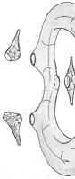
Figure 8. $(\delta,\eta)$-thick components in hyperbolic metric

4.5. Uniform bounds for the conformal factor

For $R>0$ and a cusp $P$, let ${\mathcal{O}}_{P}(R)$ denote the neighborhood $\{\zeta\mid|\zeta|<R\}$ where $\zeta$ is as in (3.21). In this subsection we fix a constant $R$ (depending only on $\delta$, $\eta$ and the stratum) such that for any hyperbolic surface $S$ and each hyperbolic cusp $P$ of $S$, the neighborhood ${\mathcal{O}}_{P}(R)$ does not intersect any of the $(\delta,\eta)$-thin components $A_{\gamma}(\eta)$, $\gamma\in\Gamma(\delta)$, and also for distinct cusps $P$ and $Q$, the neighborhoods ${\mathcal{O}}_{P}(R)$ and ${\mathcal{O}}_{Q}(R)$ are disjoint.

The following Proposition is a variant of the Theorem of K. Rafi stated in the beginning of §4.

Proposition 4.1.

Let $S=(C,q)$ be a flat surface, and let $Y$ be a $\delta$-thick component of $S$. Let $Y(\eta)$ be the corresponding $(\delta,\eta)$-thick component of $S$ (defined as in §4.4). For each $P\in Z(Y(\eta))$, let ${\mathcal{O}}_{P}(R)$ be the neighborhood of $P$ as defined in the beginning of §4.5. Then, there exists a constant $C^{\prime}$ depending only on the stratum, $\delta$, $\eta$ and $R$ such that for all $x\in Y(\eta)-\bigcup_{P\in Z(Y)}{\mathcal{O}}_{P}(R)$,

$$|\phi(q)(x)-\log\lambda(Y)|\leq C^{\prime},$$

where $\phi(q)$ is the conformal factor of $q$ defined by $g_{flat}(q)=\exp(2\phi(q))g_{hyp}$.

Proof.

The proof will be by contradiction. Suppose there is no $C^{\prime}$ satisfying the conditions of the lemma. Then there exists sequence of triples $(x_{\tau},Y_{\tau},S_{\tau})$ such that $Y_{\tau}\subset S_{\tau}$ is a $\delta$-thick subsurface, $x_{\tau}\in Y_{\tau}(\eta)$, and if we write $S_{\tau}=(C_{\tau},q_{\tau})$ then

(4.2) $$|\phi(q_{\tau})(x_{\tau})-\log\lambda(Y_{\tau})|\to\infty.$$

After passing to a subsequence, we may assume that the flat surfaces $S_{\tau}$ converge in the sense of Theorem 10. Let $C_{\infty}$, $\delta_{0}$, $C_{\infty,j}$, $Y_{\tau,j}$, $\tilde{q}_{\tau,j}$ be as in the statement of Theorem 10. One technical issue is that the constant $\delta_{0}$ (which depends on the sequence $S_{\tau}$) might not coincide with the constant $\delta>0$ which is chosen in advance; in particular, we may have $\delta_{0}<\delta$.

Since $Y_{\tau}$ is a thick component of $S_{\tau}$, for large enough $\tau$ no boundary curve of one of the $Y_{\tau,j}$ (which are all in $\Gamma(\delta_{0})$) can cross the interior of $Y_{\tau}$; therefore the subsurface $Y_{\tau}$ must be contained in one of the $Y_{\tau,j}$ where $j=j(\tau)$; however after passing to a subsequence we may assume that $j$ is fixed. Even then, we might not have $Y_{\tau}=Y_{\tau,j}$ since all we know about the boundary curves of $Y_{\tau}$ is that they have hyperbolic length at most $\delta$, while by definition, the hyperbolic length of the boundary curves of $Y_{\tau,j}$ tends to $0$ as $\tau\to\infty$. However, we claim that

(4.3) $$\limsup_{\tau\to\infty}|\log\lambda(Y_{\tau})-\log\lambda(Y_{\tau,j})|<\infty.$$

Indeed, if (4.3) failed, then (after passing to a subsequence) by [EMzRf, Lemma 4.9], the subsurface $Y_{\tau,j}$ would contain a curve $\gamma_{\tau,j}$ with the hyperbolic length of $\gamma_{\tau,j}\to 0$; this contradicts the fact that $Y_{\tau,j}\to C_{\infty,j}$ where $C_{\infty,j}$ is connected. Therefore (4.3) holds. It follows from (4.2) and (4.3) that

(4.4) $$|\phi(q_{\tau})(x_{\tau})-\log\lambda(Y_{\tau,j})|\to\infty.$$

As in Theorem 10, let

$$\tilde{q}_{\tau,j}=\lambda(Y_{\tau,j})^{-2}q_{\tau}$$

By Theorem 10, we have $\tilde{q}_{\tau,j}\to\tilde{q}_{\infty,j}$ on uniformly on compact subsets of $C_{\infty,j}$ After passing to a subsequence, we have $x_{\tau}\to x_{\infty}\in C_{\infty,j}$. Since $x_{\tau}$ stays away from $Z(Y_{\tau,j})$, $x_{\infty}\not\in Z(Y_{\infty,j})$. Also, since $x_{\tau}\in Y_{\tau,j}(\eta)$, $x_{\infty}$ is not one of the nodes. Since $\tilde{q}_{\infty,j}$ is finite and does not vanish except at ponts of $Z(Y_{\infty,j})$ and the nodes, we see that $\tilde{q}_{\infty,j}(x_{\infty})\neq 0$.

Recall that we represent the conformal factor relating the flat and hyperbolic metrics as $g_{\mathit{flat}}(q_{\tau})=\exp(2\phi(q_{\tau}))g_{\mathit{hyp}}$. Therefore,

$$\phi(\tilde{q}_{\tau,j})(x_{\tau})\to\phi(\tilde{q}_{\infty,j})(x_{\infty})\neq 0.$$

Hence,

(4.5) $$\limsup_{\tau\to\infty}|\phi(\tilde{q}_{\tau,j})(x_{\tau})|<\infty.$$

Recall that by definition $\tilde{q}_{\tau,j}:=\lambda(Y_{\tau,j})^{-2}q_{\tau}$. Note that multiplying $q_{\tau}$ by a constant factor $k$ we do not change the hyperbolic metric, $g_{\mathit{hyp}}(kq_{\tau})=g_{\mathit{hyp}}(q_{\tau})$. Thus,

(4.6) $$\phi(\tilde{q}_{\tau,j})=\phi(q_{\tau})-\log\lambda(Y_{\tau,j}).$$

Now (4.6) and (4.5) contradict (4.4). ∎

5. Analytic Riemann–Roch Theorem

This section is entirely devoted to a proof of Theorem 5. In section 5.1 we present our original proof based on the results of J. Fay [Fay].

Having seen a draft of the paper, D. Korotkin indicated us that Theorem 5 should be an immediate corollary of the holomorphic factorization formula from [KkKt2] combined with the homogeneity properties of the tau-function established in [KtZg]. We present a corresponding alternative proof in section 5.2.

5.1. Proof based on the results of J. Fay

Recall the setting of Theorem 5. Consider a flat surface $S$ of area one in a stratum of Abelian differentials or in a stratum of meromorphic quadratic differentials with at most simple poles. In the current context we are interested only in the underlying flat metric, so we forget about the choice of the vertical direction. In other words, we do not distinguish flat surfaces corresponding to Abelian differentials $\omega$ and $\exp(i\varphi)\omega$ (correspondingly quadratic differentials $q$ and $\exp(2i\varphi)q$), where $\varphi$ is a constant real number. e consider the flat surface W$S$ as a point of the quotient

$${\mathcal{H}}_{1}(m_{1},\dots,m_{n})/\operatorname{SO}(2,{\mathbb{R}})\simeq\ \operatorname{\mathbb{P}}\!{\mathcal{H}}(m_{1},\dots,m_{n})$$

or

$${\mathcal{Q}}_{1}(d_{1},\dots,d_{n})/\operatorname{SO}(2,{\mathbb{R}})\simeq\ \operatorname{\mathbb{P}}{\mathcal{Q}}_{1}(d_{1},\dots,d_{n})$$

correspondingly.

Consider a complex one-parameter family of local holomorphic deformations $S(t)$ of $S$ in the ambient stratum ${\mathcal{H}}(m_{1},\dots,m_{n})$ or ${\mathcal{Q}}(d_{1},\dots,d_{n})$ correspondingly. Denote by $z$ a flat coordinate on the initial flat surface, and by $u$ denote a flat coordinate on the deformed flat surface. The area of the deformed flat surface $S(t)$ is not unit anymore. We denote by $S^{(1)}(t)$ the flat surface of area one obtained from $S(t)$ by the proportional rescaling. Smoothing the resulting flat metric of area one as it was described in section 3.6, we get the smoothed flat metric $\rho_{\varepsilon}(u,\bar{u})|du|^{2}$.

By $\omega_{i}$, $i=1,\dots,g$, we denote local nonvanishing holomorphic sections of the Hodge bundle $H^{1,0}$, so $\det^{\frac{1}{2}}\langle\omega_{i},\omega_{j}\rangle$ is a local holomorphic section of the determinant bundle $\Lambda^{g}H^{1,0}$, and $|\det\langle\omega_{i},\omega_{j}\rangle|$ is the square of its norm induced by Hermitian metric (1.1), see (3.4).

The starting point of the proof is the following reformulation of a formula of J. Fay.

Proposition 5.1 (after J. Fay).

The following relation is valid

(5.1) $$\partial_{\bar{t}}\partial_{t}\log\det\Delta_{\mathit{flat},\varepsilon}\big{(}S^{(1)}(t)\big{)}-\partial_{\bar{t}}\partial_{t}\log|\det\langle\omega_{i},\omega_{j}\rangle|=\\ =\cfrac{1}{6\pi}\,\int_{C}\det\left(\begin{array}[]{c|c}\partial_{\bar{t}}\partial_{t}\log\rho_{\varepsilon}&\partial_{t}\partial_{\bar{u}}\log\rho_{\varepsilon}\\[-6.0pt] &\\ \hline\cr&\\[-6.0pt] \partial_{\bar{t}}\partial_{u}\log\rho_{\varepsilon}&\partial_{z}\partial_{\bar{z}}\log\rho_{\varepsilon}\end{array}\right)dx\,dy\,.$$

where the derivatives of functions of the local coordinate $u$ are evaluated at $t=0$.

Proof.

Actually, formula (5.1) above is formula (3.37) in [Fay] adjusted to our notations.

A vector bundle $L_{t}$ in formula (3.37) in [Fay] is trivial in our case. This means that the metric $h$ on it is also trivial and equals identically one: $h=1$. The same is true for the determinant $\det\langle\omega_{i},\omega_{j}\rangle_{L_{t}}$ in formula (3.37) in [Fay]; this determinant is identically equal to one in our case.

A vector bundle $K_{t}\otimes L^{\ast}_{t}$ in formula (3.37) in [Fay] becomes in our context the vector bundle $H^{1,0}$ and a basis in the fiber of this vector bundle denoted in [Fay] by $\{\omega^{\ast}_{k}\}$ becomes a basis of holomorphic 1-forms in $H^{1,0}(C(t))$, denoted in our notations by $\omega_{k}(t)$ where $C(t)$ is a Riemann surface underlying the deformed flat surface $S(t)$. Note that each $\omega_{k}(t)$ considered as a section of the holomorphic vector bundle $H^{1,0}$ is holomorphic with respect to the parameter of deformation $t$.

Note, that we represent the metric as $\rho_{\varepsilon}(u,\bar{u})\,|du|^{2}$ while in the original paper [Fay] the same metric is written as $\rho^{-2}|du|^{2}$. This explains an extra factor of $4$ in the denominator of $1/(4\pi)$ in formula (5.2) below with respect to the original formula (3.37) in [Fay].

Finally, using that

$$\rho_{\varepsilon}\partial(\rho_{\varepsilon}^{-1})=-\partial\log\rho_{\varepsilon}\,.$$

we can rewrite formula (3.37) in [Fay] in our notations as

(5.2) $$\partial_{\bar{t}}\partial_{t}\,\log\left(\cfrac{\det\Delta_{\mathit{flat},\varepsilon}\big{(}S^{(1)}(t)\big{)}}{|\det\langle\omega_{i},\omega_{j}\rangle|}\right)\ =\\ \ =\frac{1}{4\pi}\int_{S}\Big{(}(\partial_{\bar{t}}\partial_{t}\log\rho_{\varepsilon})\;(\partial_{\bar{z}}\partial_{z}\log\rho_{\varepsilon})-(\partial_{t}\partial_{\bar{u}}\log\rho_{\varepsilon})\;(\partial_{\bar{t}}\partial_{u}\log\rho_{\varepsilon})-\\ -\frac{1}{3}(\partial_{t}\partial_{\bar{t}}\log\rho_{\varepsilon})\;(\partial_{z}\partial_{\bar{z}}\log\rho_{\varepsilon})+\cfrac{1}{3}(\partial_{t}\partial_{\bar{u}}\log\rho_{\varepsilon})\;(\partial_{\bar{t}}\partial_{u}\log\rho_{\varepsilon})\Big{)}\,dx\,dy\,.$$

Simplifying the expression in the right-hand side of (5.2), we can rewrite the latter formula in the form (5.1). ∎

Lemma 5.1.

In the same setting as above the following formula is valid

(5.3) $$\partial_{\bar{t}}\partial_{t}\,\log\det\Delta_{\text{{flat}}}\big{(}S^{(1)}(t),S_{0}\big{)}\ =\\ =\ \partial_{\bar{t}}\partial_{t}\,\log|\det\langle\omega_{i},\omega_{j}\rangle|\ +\ \cfrac{1}{6\pi}\,\lim_{\varepsilon\to+0}\,\int_{C}\det\left(\begin{array}[]{c|c}\partial_{\bar{t}}\partial_{t}\log\rho_{\varepsilon}&\partial_{t}\partial_{\bar{u}}\log\rho_{\varepsilon}\\[-6.0pt] &\\ \hline\cr&\\[-6.0pt] \partial_{\bar{t}}\partial_{u}\log\rho_{\varepsilon}&\partial_{z}\partial_{\bar{z}}\log\rho_{\varepsilon}\end{array}\right)dx\,dy$$

where all derivatives of functions of the local coordinate $u$ are evaluated at $t=0$.

Proof.

Combine the latter equation with definition (3.16) of $\det\Delta_{\text{{flat}}}\big{(}S^{(1)}(t),S_{0}\big{)}$ and pass to the limit as $\varepsilon\to+0$. ∎

Now let us specify the holomorphic 1-parameter family $S(t)$ of infinitesimal deformations of the flat surface $S=S(0)$.

When the flat surface $S$ is represented by an Abelian differential $\omega$ in a stratum ${\mathcal{H}}(m_{1},\dots,m_{n})$ we consider an infinitesimal affine line $\gamma(t)$ defined in cohomological coordinates

$$(Z_{1},\dots,Z_{2g+n-1})\in H^{1}(S,\{\text{zeroes of }\omega\};{\mathbb{C}})$$

by the parametric system of equation

(5.4) $$Z_{j}(t):= a(t)Z_{j}(0)+b(t)\bar{Z}_{j}(0)\,,\quad\text{for }j=1,\dots,2g+n-1\,,$$

$$\text{where }\ a(0)=1,\ b(0)=0,\ \text{ and }\ b^{\prime}(0)\neq 0\,.$$

When the flat surface $S$ is represented by a meromorphic quadratic differential $q$ in a stratum ${\mathcal{Q}}(d_{1},\dots,d_{n})$, we consider an infinitesimal affine line $\gamma(t)$ defined in cohomological coordinates

$$(Z_{1},\dots,Z_{2g+n-2})\in H_{-}^{1}(S,\{\text{zeroes of }\hat{\omega}\};{\mathbb{C}})$$

by an analogous parametric system of equations

(5.5) $$Z_{j}(t):= a(t)Z_{j}(0)+b(t)\bar{Z}_{j}(0)\,,\quad\text{for }j=1,\dots,2g+n-2\,,$$

$$\text{where }\ a(0)=1,\ b(0)=0,\ \text{ and }\ b^{\prime}(0)\neq 0\,.$$

The next Proposition evaluates the limit in equation (5.3) for families of deformations (5.4) and (5.5).

Proposition 5.2.

In the same setting as above the following formulae hold.

For a family of deformations (5.4) of the initial flat surface $S$ inside a stratum ${\mathcal{H}}(m_{1},\dots,m_{n})$ of Abelian differentials one has:

(5.6) $$\lim_{\varepsilon\to+0}\int_{C}\det\left(\begin{array}[]{c|c}\partial_{t}\partial_{\bar{t}}\log\rho_{\varepsilon}&\partial_{t}\partial_{\bar{u}}\log\rho_{\varepsilon}\\[-6.0pt] &\\ \hline\cr&\\[-6.0pt] \partial_{\bar{t}}\partial_{u}\log\rho_{\varepsilon}&\partial_{z}\partial_{\bar{z}}\log\rho_{\varepsilon}\end{array}\right)dx\,dy=\pi\cdot\sum_{j=1}^{n}\cfrac{m_{j}(m_{j}+2)}{2(m_{j}+1)}\cdot|b^{\prime}(0)|^{2}$$

For a family of deformations (5.5) of the initial flat surface $S$ inside a stratum ${\mathcal{Q}}(d_{1},\dots,d_{n})$ of meromorphic quadratic differentials with at most simple poles one has:

(5.7) $$\lim_{\varepsilon\to+0}\int_{C}\det\left(\begin{array}[]{c|c}\partial_{t}\partial_{\bar{t}}\log\rho_{\varepsilon}&\partial_{t}\partial_{\bar{u}}\log\rho_{\varepsilon}\\[-6.0pt] &\\ \hline\cr&\\[-6.0pt] \partial_{\bar{t}}\partial_{u}\log\rho_{\varepsilon}&\partial_{z}\partial_{\bar{z}}\log\rho_{\varepsilon}\end{array}\right)dx\,dy=\pi\cdot\sum_{j=1}^{n}\cfrac{d_{j}(d_{j}+4)}{4(d_{j}+2)}\cdot|b^{\prime}(0)|^{2}$$

Proof.

We are going to show that the integral under consideration is localized into small neighborhoods of conical singularities, and that the integral over any such neighborhood depends only on the cone angle at the singularity. In particular, it does not depend on the holonomy of the flat metric, so it does not distinguish flat metrics corresponding to holomorphic 1-forms and to quadratic differentials. In other words the second formula in the statement of Proposition 5.2 is valid no matter whether a quadratic differential is or is not a global square of an Abelian differential. The first formula, thus, becomes an immediate corollary of the second one: if an Abelian differential has zeroes of degrees $m_{1},\dots,m_{n}$, the quadratic differential $\omega^{2}$ has zeroes of orders $2m_{1},\dots,2m_{n}$. Applying the second formula to this latter collection of singularities we obtain the first one.

We can represent a holomorphic deformation of the flat coordinate $z$ as follows:

$$u(z,\bar{z},t)=a(t)\,z+b(t)\,\bar{z}$$

where $t\in{\mathbb{C}}$ is a parameter of the deformation and coefficients are normalized as $a(0)=1$, $b(0)=0$, and $b^{\prime}(0)\neq 0$, see (5.4), and (5.5). We get

(5.8) $$du\wedge d\bar{u}=(a\,dz+b\,d\bar{z})\wedge(\bar{a}\,d\bar{z}+\bar{b}\,dz)=(a\bar{a}-b\bar{b})\,dz\wedge d\bar{z}$$

Computing the derivatives we get:

(5.9) $$\partial_{t}u =a^{\prime}z+b^{\prime}\bar{z} \partial_{t}\bar{u} =0$$

$$\partial_{\bar{t}}u =0 \partial_{\bar{t}}\bar{u} =\bar{a}^{\prime}\bar{z}+\bar{b}^{\prime}z$$

where $a^{\prime}=\partial_{t}\,a(t)$ and $b^{\prime}=\partial_{t}\,b(t)$.

It would be convenient to introduce the following notation: $G(t,\bar{t}):=(a\bar{a}-b\bar{b})^{-1}$. Computing the derivatives of $G$ we get:

$$\partial_{t}\,G =-G^{2}\cdot(a^{\prime}\bar{a}-b^{\prime}\bar{b}) \partial_{t}G\big{|}_{t=0} =-a^{\prime}(0)$$

(5.10) $$\partial_{\bar{t}}\,G =-G^{2}\cdot(a\bar{a}^{\prime}-b\bar{b}^{\prime}) \partial_{\bar{t}}G\big{|}_{\bar{t}=0} =-\bar{a}^{\prime}(0)$$

$$\partial_{t}\partial_{\bar{t}}\,G =2G^{3}\cdot(a^{\prime}\bar{a}-b^{\prime}\bar{b})(a\bar{a}^{\prime}-b\bar{b}^{\prime})-$$

$$\qquad-G^{2}(a^{\prime}\bar{a}^{\prime}-b^{\prime}\bar{b}^{\prime}) \partial_{t}\partial_{\bar{t}}G\big{|}_{t=0} =a^{\prime}(0)\bar{a}^{\prime}(0)+b^{\prime}(0)\bar{b}^{\prime}(0)$$

Consider a neighborhood ${\mathcal{O}}$ of a conical singularity $P$ of order $d$ on the initial flat surface $S$. Recall that the local coordinate $w$ in ${\mathcal{O}}$ is defined by the equation $(dz)^{2}=w^{d}\,(dw)^{2}$, see (3.13). The smoothed metric $g_{\mathit{flat},\varepsilon}$ was defined in ${\mathcal{O}}$ as $g_{\mathit{flat},\varepsilon}=\rho_{\mathit{flat},\varepsilon}(|w|)\,|dw|^{2}$, where the function $\rho_{\mathit{flat},\varepsilon}$ is defined in equation (3.15). In the flat coordinate $z$ the smoothed metric has the form $g_{\mathit{flat},\varepsilon}=\rho_{\varepsilon}(|z|)\,|dz|^{2}$, where the function $\rho_{\varepsilon}(|z|)$ is defined by the equation

$$\rho_{\mathit{flat},\varepsilon}(|w|)\,|dw|^{2}=\rho_{\varepsilon}(|z|)\,|dz|^{2}$$

A simple calculation shows that

(5.11) $$\rho_{\varepsilon}(r)=\begin{cases}1&,\text{ when }r\geq\varepsilon\\ \left(\frac{2}{d+2}\right)^{2}\cdot r^{-\frac{2d}{d+2}}&,\text{ when }0<r\leq\varepsilon^{\prime}\,.\end{cases}$$

Finally, it would be convenient to make one more substitution, representing the smoothed metric in ${\mathcal{O}}$ as

$$\rho_{\varepsilon}(|z|)\,|dz|^{2}=\exp\big{(}2\varphi_{\varepsilon}(|z|^{2})\big{)}\,|dz|^{2}\,.$$

The above definition of $\varphi_{\varepsilon}$ implies that

(5.12) $$\varphi_{\varepsilon}(s)=\begin{cases}0&,\text{ when }s\geq\varepsilon^{2}\\ \log\left(\frac{2}{d+2}\right)-\frac{d}{2(d+2)}\log s&,\text{ when }0<s\leq(\varepsilon^{\prime})^{2}\,.\end{cases}$$

We will need below the following immediate implication of the above expression:

(5.13) $$\varphi_{\varepsilon}^{\prime}(s)\cdot s=\begin{cases}0&\text{ when }s\geq\varepsilon^{2}\\ -\frac{d}{2(d+2)}&\text{ when }0<s\leq(\varepsilon^{\prime})^{2}\end{cases}$$

Consider now a neighborhood ${\mathcal{O}}$ of a conical singularity $P$ on the deformed flat surface $S^{(1)}(t)$ with normalized metric. It follows from (5.8) that smoothed metric $\rho_{\varepsilon}(u,\bar{u})|du|^{2}$ has the form

$$\rho_{\varepsilon}(u,\bar{u})=\exp\big{(}2\varphi_{\varepsilon}(u\bar{u}G)\big{)}\cdot G(t,\bar{t})$$

in such neighborhood. The second factor $G(t,\bar{t})$ in the above expression is responsible for the normalization

$$\operatorname{area}\big{(}S^{(1)}(t)\big{)}=1$$

of the total area of the deformed flat surface $S(t)$. Passing to the logarithm we get

$$\log\rho_{\varepsilon}(u,\bar{u})=2\varphi_{\varepsilon}(u\bar{u}G)+\log G\,.$$

Now everything is ready to compute the entries of the matrix

$$\left(\begin{array}[]{c|c}\partial_{t}\partial_{\bar{t}}\log\rho_{\varepsilon}&\partial_{t}\partial_{\bar{u}}\log\rho_{\varepsilon}\\[-6.0pt] &\\ \hline\cr&\\[-6.0pt] \partial_{\bar{t}}\partial_{u}\log\rho_{\varepsilon}&\partial_{z}\partial_{\bar{z}}\log\rho_{\varepsilon}\end{array}\right).$$

Entry $\left(\begin{array}[]{c|c}\bullet&\phantom{\bullet}\\ \hline\cr&\end{array}\right).$

Evaluating the first derivative $\partial_{\bar{t}}\log\rho_{\varepsilon}$ we get

$$\partial_{\bar{t}}\log\rho_{\varepsilon}=\partial_{\bar{t}}\,\Big{(}2\varphi_{\varepsilon}(u\bar{u}G)+\log G(t,\bar{t})\Big{)}=2\varphi_{\varepsilon}^{\prime}\cdot\left(u\cfrac{\partial\bar{u}}{\partial\bar{t}}\,G+u\bar{u}\,\cfrac{\partial G}{\partial\bar{t}}\right)+\cfrac{\partial G}{\partial\bar{t}}\cdot\cfrac{1}{G}$$

Passing to the second derivative we obtain

$$\partial_{t}\partial_{\bar{t}}\log\rho_{\varepsilon}=2\varphi_{\varepsilon}^{\prime\prime}\cdot\left(\bar{u}\cfrac{\partial u}{\partial t}\,G+u\bar{u}\,\cfrac{\partial G}{\partial t}\right)\left(u\cfrac{\partial\bar{u}}{\partial\bar{t}}\;G+u\bar{u}\,\cfrac{\partial G}{\partial\bar{t}}\right)+\\ +2\varphi_{\varepsilon}^{\prime}\cdot\left(\cfrac{\partial u}{\partial t}\,\cfrac{\partial\bar{u}}{\partial\bar{t}}\cdot G+\bar{u}\,\cfrac{\partial u}{\partial t}\,\cfrac{\partial G}{\partial\bar{t}}+u\,\cfrac{\partial\bar{u}}{\partial\bar{t}}\,\cfrac{\partial G}{\partial t}+u\bar{u}\,\cfrac{\partial^{2}G}{\partial t\,\partial\bar{t}}\right)+\cfrac{\partial^{2}G}{\partial t\partial\bar{t}}\,\cdot\cfrac{1}{G}-\cfrac{\partial G}{\partial t}\,\cfrac{\partial G}{\partial\bar{t}}\cdot\cfrac{1}{G^{2}}$$

Applying formulae (5.9) we evaluate the above expression at $t=0$ getting:

$$2\varphi_{\varepsilon}^{\prime\prime}\cdot\left((a^{\prime}z+b^{\prime}\bar{z})\bar{z}\cdot G+z\bar{z}\,\cfrac{\partial G}{\partial t}\right)\left((\bar{a}^{\prime}\bar{z}+\bar{b}^{\prime}z)z\cdot G+z\bar{z}\,\cfrac{\partial G}{\partial\bar{t}}\right)+\\ +\;2\varphi_{\varepsilon}^{\prime}\cdot\Bigg{(}(a^{\prime}z+b^{\prime}\bar{z})(\bar{a}^{\prime}\bar{z}+\bar{b}^{\prime}z)\cdot G+(a^{\prime}z+b^{\prime}\bar{z})\bar{z}\,\cfrac{\partial G}{\partial\bar{t}}\;+\\ +(\bar{a}^{\prime}\bar{z}+\bar{b}^{\prime}z)z\,\cfrac{\partial G}{\partial t}+z\bar{z}\,\cfrac{\partial^{2}G}{\partial t\,\partial\bar{t}}\Bigg{)}\;+\\ +\;\cfrac{\partial^{2}G}{\partial t\partial\bar{t}}\,\cdot\cfrac{1}{G}-\cfrac{\partial G}{\partial t}\,\cfrac{\partial G}{\partial\bar{t}}\cdot\cfrac{1}{G^{2}}$$

Applying formulae (5.10) for derivatives of $G$ at $t=0$ we can rewrite the latter expression as

$$2\varphi_{\varepsilon}^{\prime\prime}\cdot\Big{(}(a^{\prime}z+b^{\prime}\bar{z})\bar{z}\cdot 1+z\bar{z}\cdot(-a^{\prime})\Big{)}\Big{(}(\bar{a}^{\prime}\bar{z}+\bar{b}^{\prime}z)z\cdot 1+z\bar{z}\cdot(-\bar{a}^{\prime})\Big{)}+\\ +2\varphi_{\varepsilon}^{\prime}\cdot\Big{(}(a^{\prime}z+b^{\prime}\bar{z})(\bar{a}^{\prime}\bar{z}+\bar{b}^{\prime}z)\cdot 1+(a^{\prime}z+b^{\prime}\bar{z})\bar{z}\,(-\bar{a}^{\prime})+\\ +(\bar{a}^{\prime}\bar{z}+\bar{b}^{\prime}z)z(-a^{\prime})+z\bar{z}(a^{\prime}\bar{a}^{\prime}+b^{\prime}\bar{b}^{\prime})\Big{)}+\\ +(a^{\prime}\bar{a}^{\prime}+b^{\prime}\bar{b}^{\prime})\cdot 1-(-a^{\prime})(-\bar{a}^{\prime})\cdot 1$$

Simplifying the latter expression we get

(5.14) $$\partial_{t}\partial_{\bar{t}}\log\rho_{\varepsilon}=b^{\prime}\bar{b}^{\prime}\Big{(}2\varphi_{\varepsilon}^{\prime\prime}\cdot(z\bar{z})^{2}+4\varphi^{\prime}\cdot z\bar{z}+1\Big{)}$$

Entry $\left(\begin{array}[]{c|c}\phantom{\bullet}&\phantom{\bullet}\\ \hline\cr&\bullet\end{array}\right).$

For this entry of the determinant we have

$$\partial_{z}\partial_{\bar{z}}\log\rho_{\varepsilon}=2\varphi_{\varepsilon}^{\prime\prime}\cdot\left(\bar{u}\cfrac{\partial u}{\partial z}+u\cfrac{\partial\bar{u}}{\partial z}\right)\left(\bar{u}\cfrac{\partial u}{\partial\bar{z}}+u\cfrac{\partial\bar{u}}{\partial\bar{z}}\right)G^{2}+2\varphi_{\varepsilon}^{\prime}\cdot\left(\cfrac{\partial u}{\partial\bar{z}}\,\cfrac{\partial\bar{u}}{\partial z}+\cfrac{\partial u}{\partial z}\,\cfrac{\partial\bar{u}}{\partial\bar{z}}\right)G$$

Applying (5.9) we can evaluate the above expression at $t=0$ which leads to

$$\partial_{z}\partial_{\bar{z}}\log\rho_{\varepsilon}=2\varphi_{\varepsilon}^{\prime\prime}\cdot z\bar{z}\cdot G^{2}(0)+2\varphi_{\varepsilon}^{\prime}\cdot 1\cdot G(0)=2(\varphi_{\varepsilon}^{\prime\prime}\cdot z\bar{z}+\varphi_{\varepsilon}^{\prime})$$

Product of diagonal terms $\left(\begin{array}[]{c|c}\bullet&\\ \hline\cr&\bullet\end{array}\right).$

Taking into consideration (5.14) we obtain the following value for the diagonal product in our determinant:

(5.15) $$\partial_{t}\partial_{\bar{t}}\log\rho_{\varepsilon}\cdot\partial_{z}\partial_{\bar{z}}\log\rho_{\varepsilon}=2b^{\prime}\bar{b}^{\prime}\cdot\Big{(}2\varphi_{\varepsilon}^{\prime\prime}\cdot(z\bar{z})^{2}+4\varphi_{\varepsilon}^{\prime}\cdot z\bar{z}+1\Big{)}\Big{(}\varphi_{\varepsilon}^{\prime\prime}\cdot z\bar{z}+\varphi_{\varepsilon}^{\prime}\Big{)}$$

Entry $\left(\begin{array}[]{c|c}\phantom{\bullet}&\bullet\\ \hline\cr&\end{array}\right).$

For the first derivative $\partial_{\bar{u}}\log\rho_{\varepsilon}$ we get

$$\partial_{\bar{u}}\log\rho_{\varepsilon}=2\varphi_{\varepsilon}^{\prime}\cdot u\cdot G$$

For the second derivative we obtain:

$$\partial_{t}\partial_{\bar{u}}\log\rho_{\varepsilon}=2\varphi_{\varepsilon}^{\prime\prime}\cdot\left(\bar{u}\,\cfrac{\partial u}{\partial t}\,G+u\bar{u}\,\cfrac{\partial G}{\partial t}\right)\cdot u\cdot G+2\varphi_{\varepsilon}^{\prime}\cdot\left(\cfrac{\partial u}{\partial t}\,G+u\,\cfrac{\partial G}{\partial t}\right)$$

Evaluating the above second derivative at $t=0$ using (5.9) and (5.10) we proceed as

(5.16) $$\partial_{t}\partial_{\bar{u}}\log\rho_{\varepsilon}=2\varphi_{\varepsilon}^{\prime\prime}\cdot\Big{(}\bar{z}\cdot(a^{\prime}z+b^{\prime}\bar{z})\cdot 1+z\bar{z}\cdot(-a^{\prime})\Big{)}\cdot z\cdot 1+\\ +2\varphi_{\varepsilon}^{\prime}\cdot\Big{(}(a^{\prime}z+b^{\prime}\bar{z})\cdot 1+z\cdot(-a^{\prime})\Big{)}=2b^{\prime}\bar{z}\cdot(\varphi_{\varepsilon}^{\prime\prime}\cdot z\bar{z}+\varphi_{\varepsilon}^{\prime})$$

Entry $\left(\begin{array}[]{c|c}&\phantom{\bullet}\\ \hline\cr\bullet&\end{array}\right).$

Analogously, for the first derivative $\partial_{u}\log\rho_{\varepsilon}$ we get

$$\partial_{u}\log\rho_{\varepsilon}=2\varphi_{\varepsilon}^{\prime}\cdot\bar{u}\cdot G$$

and for the second derivative we obtain:

$$\partial_{\bar{t}}\partial_{u}\log\rho_{\varepsilon}=2\varphi_{\varepsilon}^{\prime\prime}\cdot\left(u\,\cfrac{\partial\bar{u}}{\partial\bar{t}}\;G+u\bar{u}\,\cfrac{\partial G}{\partial\bar{t}}\right)\cdot\bar{u}\cdot G+2\varphi_{\varepsilon}^{\prime}\cdot\left(\cfrac{\partial\bar{u}}{\partial\bar{t}}\,G+\bar{u}\,\cfrac{\partial G}{\partial\bar{t}}\right)$$

Evaluating the above expression at $t=0$ using (5.9) and (5.10) we complete the calculation as

(5.17) $$\partial_{\bar{t}}\partial_{u}\log\rho_{\varepsilon}=2\varphi_{\varepsilon}^{\prime\prime}\cdot\Big{(}z\cdot(\bar{a}^{\prime}\bar{z}+\bar{b}^{\prime}z)\cdot 1+z\bar{z}\cdot(-\bar{a}^{\prime})\Big{)}\cdot\bar{z}\cdot 1\;+\\ +\;2\varphi_{\varepsilon}^{\prime}\cdot\Big{(}(\bar{a}^{\prime}\bar{z}+\bar{b}^{\prime}z)\cdot 1+\bar{z}\cdot(-\bar{a}^{\prime})\Big{)}=2\bar{b}^{\prime}z\cdot(\varphi_{\varepsilon}^{\prime\prime}\cdot z\bar{z}+\varphi_{\varepsilon}^{\prime})$$

Product of diagonal terms $\left(\begin{array}[]{c|c}&\bullet\\ \hline\cr\bullet&\end{array}\right).$

Combining (5.16) and (5.17) we obtain the following value for the anti diagonal product in our determinant:

(5.18) $$\partial_{t}\partial_{\bar{u}}\log\rho_{\varepsilon}\cdot\partial_{\bar{t}}\partial_{u}\log\rho_{\varepsilon}=4b^{\prime}\bar{b}^{\prime}\cdot z\bar{z}\cdot\big{(}\varphi_{\varepsilon}^{\prime\prime}\cdot z\bar{z}+\varphi_{\varepsilon}^{\prime}\big{)}^{2}$$

Finally, combining (5.15) and (5.18) we obtain the desired value of the determinant:

(5.19) $$\det\left(\begin{array}[]{c|c}\partial_{t}\partial_{\bar{t}}\log\rho_{\varepsilon}&\partial_{t}\partial_{\bar{u}}\log\rho_{\varepsilon}\\[-6.0pt] &\\ \hline\cr&\\[-6.0pt] \partial_{\bar{t}}\partial_{u}\log\rho_{\varepsilon}&\partial_{z}\partial_{\bar{z}}\log\rho_{\varepsilon}\end{array}\right)=\\ =2b^{\prime}\bar{b}^{\prime}\cdot\big{(}\varphi_{\varepsilon}^{\prime\prime}\cdot z\bar{z}+\varphi_{\varepsilon}^{\prime}\big{)}\cdot\Bigg{(}\big{(}2\varphi_{\varepsilon}^{\prime\prime}\cdot(z\bar{z})^{2}+4\varphi_{\varepsilon}^{\prime}\cdot z\bar{z}+1\big{)}-2z\bar{z}\cdot\big{(}\varphi_{\varepsilon}^{\prime\prime}\cdot z\bar{z}+\varphi_{\varepsilon}^{\prime}\big{)}\Bigg{)}=\\ =2b^{\prime}\bar{b}^{\prime}\cdot\Big{(}2\varphi_{\varepsilon}^{\prime}\cdot\varphi_{\varepsilon}^{\prime\prime}\cdot(z\bar{z})^{2}+2(\varphi_{\varepsilon}^{\prime})^{2}\cdot z\bar{z}+\varphi_{\varepsilon}^{\prime\prime}\cdot z\bar{z}+\varphi_{\varepsilon}^{\prime}\Big{)}$$

Now we need to integrate the above expression over the flat surface $S$. First note that outside of small neighborhoods of conical singularities, the smoothed metric $\rho_{\varepsilon}(z,\bar{z})|dz|^{2}$ coincides with the original flat metric, so for such values of $x,y$ we have $\rho_{\varepsilon}=1$ and hence, for such values of $(x,y)$ we have $\log\rho_{\varepsilon}(x,y)=0$. This observation proves that

(5.20) $$\int_{S}\det\left(\begin{array}[]{c|c}\partial_{t}\partial_{\bar{t}}\log\rho_{\varepsilon}&\partial_{t}\partial_{\bar{u}}\log\rho_{\varepsilon}\\[-6.0pt] &\\ \hline\cr&\\[-6.0pt] \partial_{\bar{t}}\partial_{u}\log\rho_{\varepsilon}&\partial_{z}\partial_{\bar{z}}\log\rho_{\varepsilon}\end{array}\right)\;dx\,dy\ =\\ =\sum_{j=1}^{n}\int_{{\mathcal{O}}_{j}(\varepsilon)}2b^{\prime}\bar{b}^{\prime}\cdot\Big{(}2\varphi_{\varepsilon}^{\prime}\cdot\varphi_{\varepsilon}^{\prime\prime}\cdot(z\bar{z})^{2}+2(\varphi_{\varepsilon}^{\prime})^{2}\cdot z\bar{z}+\varphi_{\varepsilon}^{\prime\prime}\cdot z\bar{z}+\varphi_{\varepsilon}^{\prime}\Big{)}\;dx\,dy\;,$$

where the sum is taken over all conical points $P_{1},\dots,P_{n}$. (We did not introduce separate notations for flat coordinates in the neighborhoods of different conical points).

Using the definition (5.12) of $\varphi_{\varepsilon}(s)$ we can rewrite the expression which we integrate in terms of a single variable $s=z\bar{z}=|z|^{2}$ as follows:

(5.21) $$2\varphi_{\varepsilon}^{\prime}\cdot\varphi_{\varepsilon}^{\prime\prime}\cdot(z\bar{z})^{2}+2(\varphi_{\varepsilon}^{\prime})^{2}\cdot z\bar{z}+\varphi_{\varepsilon}^{\prime\prime}\cdot z\bar{z}+\varphi_{\varepsilon}^{\prime}=\\ =2\varphi_{\varepsilon}^{\prime}(s)\cdot\varphi_{\varepsilon}^{\prime\prime}(s)\cdot s^{2}+2(\varphi_{\varepsilon}^{\prime}(s))^{2}\cdot s+\varphi_{\varepsilon}^{\prime\prime}(s)\cdot s+\varphi_{\varepsilon}^{\prime}(s)=:\Phi_{\varepsilon}(s)$$

Recall that in the flat coordinate $z$ a small neighborhood of a conical singularity of order $d$ is glued from $d+2$ metric half-discs. Taking into consideration angular symmetry of the expression which we integrate and passing through polar coordinates in our integral we can reduce integration over a $d+2$ metric half-discs to integration over a segment:

(5.22) $$2b^{\prime}\bar{b}^{\prime}\int_{{\mathcal{O}}_{j}(\varepsilon)}\Phi_{\varepsilon}(z\bar{z})\,dx\,dy\ =\ 2(d+2)b^{\prime}\bar{b}^{\prime}\int_{\begin{subarray}{c}|z|\leq\varepsilon\\ \operatorname{Re}(x)\geq 0\end{subarray}}\Phi_{\varepsilon}(r^{2})\,r\,dr\,d\theta\ =\\ =\ (d+2)\pi\cdot b^{\prime}\bar{b}^{\prime}\int_{0}^{\varepsilon^{2}}\Phi_{\varepsilon}(s)\,ds$$

Finally, observe that it is easy to find an antiderivative for $\Phi_{\varepsilon}(s)$, namely:

$$\Phi_{\varepsilon}(s)=\left(\big{(}\varphi^{\prime}(s)\big{)}^{2}\cdot s^{2}+\varphi^{\prime}(s)\cdot s\right)^{\prime}$$

which implies, that

$$\int_{0}^{\varepsilon^{2}}\Phi_{\varepsilon}(s)\,ds=\big{(}\varphi_{\varepsilon}^{\prime}(s)\cdot s\big{)}^{2}\Big{|}^{\varepsilon^{2}}_{+0}\ +\ \varphi_{\varepsilon}^{\prime}(s)\cdot s\Big{|}^{\varepsilon^{2}}_{+0}$$

Using the properties (5.13) of $\varphi_{\varepsilon}(s)$ we get

$$\int_{0}^{\varepsilon^{2}}\Phi_{\varepsilon}(s)\,ds=\left(0-\left(-\frac{d}{2(d+2)}\right)^{2}\right)+\left(0-\left(-\frac{d}{2(d+2)}\right)\right)=\frac{d(d+4)}{4(d+2)^{2}}$$

Plug the value of the integral obtained in the right-hand side of the above formula in equation (5.22) and combine the result with (5.20) and with (5.21). The resulting expression coincides with equation (5.7) in the statement of Proposition 5.2. As we have already indicated above, relation (5.6) follows immediately from equation (5.7) and from the fact that the integral is supported on small neighborhoods of the conical points of the metric. Proposition 5.2 is proved. ∎

Lemma 5.2.

In the same setting as above the following formulae hold.

For a family of deformations (5.4) of the initial flat surface $S$ in a stratum ${\mathcal{H}}(m_{1},\dots,m_{n})$ of Abelian differentials one has:

(5.23) $$\partial_{\bar{t}}\partial_{t}\,\log\det\Delta_{\text{{flat}}}(S,S_{0})\ =\\ =\ \partial_{\bar{t}}\partial_{t}\,\log|\det\langle\omega_{i},\omega_{j}\rangle|\ +\ \frac{1}{12}\cdot\sum_{j=1}^{n}\cfrac{m_{j}(m_{j}+2)}{(m_{j}+1)}\cdot|b^{\prime}(0)|^{2}$$

For a family of deformations (5.5) of the initial flat surface $S$ inside a stratum ${\mathcal{Q}}(d_{1},\dots,d_{n})$ of meromorphic quadratic differentials with at most simple poles one has:

(5.24) $$\partial_{\bar{t}}\partial_{t}\,\log\det\Delta_{\text{{flat}}}(S,S_{0})\ =\\ =\ \partial_{\bar{t}}\partial_{t}\,\log|\det\langle\omega_{i},\omega_{j}\rangle|\ +\ \frac{1}{24}\cdot\sum_{j=1}^{n}\cfrac{d_{j}(d_{j}+4)}{(d_{j}+2)}\cdot|b^{\prime}(0)|^{2}$$

Proof.

Plugging expressions (5.6) and (5.7) obtained in Proposition 5.2 into formula (5.3) from Lemma 5.1 we get the relations (5.23) and (5.24) from above. ∎

Consider the natural projection

$$p:{\mathcal{H}}(m_{1},\dots,m_{n})\to\operatorname{\mathbb{P}}\!{\mathcal{H}}(m_{1},\dots,m_{n})\,.$$

Families of deformations (5.4) and (5.5) are chosen in such a way that the resulting infinitesimal affine line $\gamma(t)$ defined by equation (5.4) in the stratum ${\mathcal{H}}(m_{1},\dots,m_{n})$ (correspondingly by equation (5.5) in the stratum ${\mathcal{Q}}(d_{1},\dots,d_{n})$) projects to the Teichmüller disc passing through $p(S)$. We will show below that the projection map $p$ from $\gamma(t)$ to the Teichmüller disc is nondegenerate in the neighborhood of $t=0$. Thus, we can induce the canonical hyperbolic metric of curvature $-4$ to $\gamma(t)$.

Lemma 5.3.

The canonical hyperbolic metric of curvature $-4$ on the Teichmüller disc induced to the infinitesimal complex curve $\gamma(t)$ under the projection $p$ has the form

$$|b^{\prime}(0)|^{2}\,|dt|^{2}$$

at the point $t=0$.

In particular, the Laplacian of the induced hyperbolic metric of curvature $-4$ on $\gamma(t)$ satisfies the relation

(5.25) $$|b^{\prime}(0)|^{2}\cdot\cfrac{1}{4}\,\,\Delta_{\mathit{Teich}}\Big{|}_{t=0}=\frac{\partial^{2}}{\partial t\,\partial\overline{t}}\Big{|}_{t=0}$$

at the point $t=0$.

Proof.

We prove the Lemma for a flat surface corresponding to an Abelian differential; for a flat surface corresponding to a meromorphic quadratic differentials with at most simple pole the proof is completely analogous.

Choose a pair of independent integer cycles $c_{1},c_{2}\in H_{1}(C,\mathbb{Z})$ such that $c_{1}\circ c_{2}=1$, and transport them to all surfaces $C(t)$ (we assume that $\gamma(t)$ stays in a tiny neighborhood of the initial point, so we would not have any ambiguity in doing so). Consider the corresponding periods of $\omega(t)$,

$$A(t):=\int_{c_{1}}\omega(t)\qquad B(t):=\int_{c_{2}}\omega(t)\,.$$

By definition of the family of deformations we get

$$A(t) =a(t)A+b(t)\bar{A}$$

$$B(t) =a(t)B+b(t)\bar{B}\,,$$

where $A=A(0)$ and $B=B(0)$ are the corresponding periods of the initial Abelian differential $\omega$. Define

$$\zeta(t):=\frac{B(t)}{A(t)}=\frac{a(t)B+b(t)\bar{B}}{a(t)A+b(t)\bar{A}}\,.$$

At the first glance this definition of the hyperbolic coordinate $\zeta(t)$ depends on the choice of a pair of cycles $c_{1},c_{2}$, and on the values of the periods of the initial Abelian differential. However, it would be clear from the proof that the induced hyperbolic metric does not depend on this choice. Basically, the situation is the same as in the case of flat tori, see Example 3.1 in section 3.1.

Consider now the hyperbolic half-plane ${\mathbb{H}}^{2}$ endowed with the canonical metric $\cfrac{|d\zeta|^{2}}{4|\operatorname{Im}\zeta|^{2}}$ of curvature $-4$. Let us compute the induced metric in the coordinate $t$.

Clearly

$$\operatorname{Im}\zeta(0)=\operatorname{Im}\frac{B}{A}\,.$$

Computing the derivative at $t=0$ we get

$$\frac{\partial\zeta}{\partial t}\Big{|}_{t=0}=b^{\prime}(0)\,\frac{\bar{B}A-B\bar{A}}{A^{2}}\,.$$

Thus

$$\frac{\partial\zeta}{\partial t}\frac{\partial\bar{\zeta}}{\partial\bar{t}}\Big{|}_{t=0}=-b^{\prime}(0)\bar{b}^{\prime}(0)\,\left(\frac{\bar{B}A-B\bar{A}^{\phantom{!}}}{A\bar{A}}\right)^{2}=4|b^{\prime}(0)|^{2}\,\left(\operatorname{Im}\frac{B}{A}\right)^{2}=\\ =4|b^{\prime}(0)|^{2}\,\operatorname{Im}^{2}\zeta(0)\,.$$

Hence, the hyperbolic metric has the following form in coordinates $t$ at $t=0$

$$\frac{|d\zeta|^{2}}{4(\operatorname{Im}\zeta)^{2}}\Bigg{|}_{\zeta(0)}=\frac{\partial\zeta}{\partial t}\frac{\partial\bar{\zeta}}{\partial\bar{t}}\,\frac{|dt|^{2}}{4(\operatorname{Im}\zeta(t))^{2}}\Bigg{|}_{t=0}=\\ =4|b^{\prime}(0)|^{2}\,\operatorname{Im}^{2}\zeta(0)\frac{|dt|^{2}}{4(\operatorname{Im}\zeta(0))^{2}}=|b^{\prime}(0)|^{2}\,|dt|^{2}$$

This implies that the Laplacian of this metric at $t=0$ is expressed as

$$\Delta_{\mathit{Teich}}=\cfrac{4}{|b^{\prime}(0)|^{2}}\,\,\frac{\partial^{2}}{\partial t\,\partial\overline{t}}\,.$$

∎

Proof of Theorem 5.

Plug the expression (5.25) for $\partial_{t}\bar{\partial}_{t}$ obtained in Lemma 5.3 into formulae (5.23) and (5.24) obtained in Lemma 5.2. Dividing all the terms of the resulting equality by the common factor $|b^{\prime}(0)|$ (which is nonzero by the definition of the family of deformations) we obtain the relations equivalent to the desired relations (3.17) and (3.18) in Theorem 5. ∎

5.2. Alternative proof based on results of A. Kokotov, D. Korotkin and P. Zograf

By assumption the initial flat surface $S=S(0)$ has area one. However, the area of the flat surface $S(t)$ in family (5.4) or in family (5.5) varies in $t$. Define the function

$$k(t,\bar{t}):=\operatorname{Area}\big{(}S(t)\big{)}^{-\frac{1}{2}}\,.$$

We shall need the following technical Lemma concerning this function.

Lemma 5.4.

One has the following expression for the partial derivative of $k(t,\bar{t})$ at $t=0$:

(5.26) $$\frac{\partial^{2}\log k(t,\bar{t})}{\partial t\,\partial\overline{t}}\Big{|}_{t=0}=\frac{1}{2}\,|b^{\prime}(0)|^{2}$$

Proof.

Relation (5.8) implies that:

$$\operatorname{Area}\big{(}S(t)\big{)}=(a\bar{a}-b\bar{b})\,,$$

so we get the following expression for the function $k(t,\bar{t})$:

$$k(t,\bar{t})=(a\bar{a}-b\bar{b})^{-\frac{1}{2}}\,.$$

Computing the value of the second derivative at $t=0$, we get

$$\frac{\partial^{2}\log k(t,\bar{t})}{\partial t\,\partial\overline{t}}\Bigg{|}_{t=0}=\frac{1}{2}\,|b^{\prime}(0)|^{2}\,,$$

where we used the conventions chosen above: $a(0)=1$ and $b(0)=0$. ∎

The proof of Theorem 5 can be derived from the following formula due to A. Kokotov, D. Korotkin (formula (1.10) in [KkKt2]). Denote by $\det\Delta^{|\omega|^{2}}$ the regularized determinant of the Laplace operator in the flat metric defined as in [KkKt2] by a holomorphic form $\omega\in{\mathcal{H}}(m_{1},\dots,m_{n})$. It is defined for flat surfaces of arbitrary area. For $\omega\in{\mathcal{H}}_{1}(m_{1},\dots,m_{n})$ the determinant $\det\Delta^{|\omega|^{2}}$ differs from $\det\Delta_{\text{{flat}}}\left(S(\omega),S_{0}\right)$ by a multiplicative constant depending only on the choice of the base surface $S_{0}$.

Theorem (A. Kokotov, D. Korotkin [KkKt2]).

For any flat surface in any stratum of Abelian differentials the following formula of holomorphic factorization holds:

(5.27) $$\det\Delta^{|\omega|^{2}}=\mathit{const}\cdot\operatorname{Area}(C,\omega)\cdot\det(\operatorname{Im}B)\cdot|\tau(C,\omega)|^{2}\,,$$

where $B$ is the matrix of $B$-periods and $\tau(C,\omega)$ is a flat section of a holomorphic line bundle over the ambient stratum ${\mathcal{H}}(m_{1},\dots,m_{n})$ of Abelian differentials.

Moreover (see [KtZg]), $\tau(S,\omega)$ is homogeneous in $\omega$ of degree $p$, where

(5.28) $$p=\frac{1}{12}\sum_{i=1}^{n}\frac{m_{i}(m_{i}+2)}{m_{i}+1}\,.$$

In other words, for any nonzero complex number $k$ one has

(5.29) $$\tau(C,k\omega)=k^{p}\tau(C,\omega)$$

Remark 5.1.

Note that the “Bergman $\tau$-function” $\tau(C,\omega)$ is, actually, a flat section of a certain local system over the stratum ${\mathcal{H}}(m_{1},\dots,m_{n})$, see Definition 3 in [KkKt2]. Such a section is defined up to a constant factor. However, in the calculation below the $\tau$-function is present only in the expression $\frac{\partial^{2}}{\partial t\,\partial\overline{t}}\log(|\tau(C,\omega)|^{2})$ which does not depend on the choice of the particular flat section. (See section 3.1 in [KkKt2] for more details.)

Alternative proof of Theorem 5.

Note that $\operatorname{Im}B(t)$ depends only on the underlying Riemann surface $C(t)$; in particular, rescaling $\omega(t)$ proportionally, we do not change $\operatorname{Im}B(t)$.

Applying formula (5.27) to the normalized Abelian differential $k(t,\bar{t})\omega(t)$, which defines a flat surface $S^{(1)}(t,\bar{t})$ of unit area, we get

$$\det\Delta_{\text{{flat}}}\left(S^{(1)}(t),S_{0}\right)=\mathit{const}\cdot 1\cdot\det\big{(}\operatorname{Im}B(t)\big{)}\cdot\bigg{|}\tau\bigg{(}C(t),k(t,\bar{t})\omega(t)\bigg{)}\bigg{|}^{2}\ =\\ =\ \mathit{const}\cdot\det(\operatorname{Im}B(t))\cdot k^{2p}(t,\bar{t})\cdot|\tau(C,\omega(t))|^{2}\,,$$

where we used homogeneity (5.29) of $\tau$ to get the latter expression. Passing to logarithms of the above expressions, applying $\frac{\partial^{2}}{\partial t\,\partial\overline{t}}$, taking into consideration that $\tau\big{(}C(t),\omega(t)\big{)}$ is a holomorphic function, and using relations (5.26) and (5.28) we get

(5.30) $$\frac{\partial^{2}}{\partial t\,\partial\overline{t}}\log|\det\Delta_{\text{{flat}}}(S(t),S_{0})|=\\ =\frac{\partial^{2}}{\partial t\,\partial\overline{t}}\log|\det\operatorname{Im}B|+\frac{1}{12}\sum_{i=1}^{n}\frac{m_{i}(m_{i}+2)}{m_{i}+1}\,|b^{\prime}(0)|^{2}\,.$$

It remains to note that

$$|\det\langle\omega_{i}(t),\omega_{j}(t)\rangle|\,=\,|\text{holomorphic function of }t|\cdot\operatorname{Im}B(t)\,.$$

Thus,

$$\frac{\partial^{2}}{\partial t\,\partial\overline{t}}\log|\det\langle\omega_{i}(t),\omega_{j}(t)\rangle|=\frac{\partial^{2}}{\partial t\,\partial\overline{t}}\log|\det\operatorname{Im}B(t)|\,.$$

Applying the latter remark to expression (5.30), dividing the result by $|b^{\prime}(0)|^{2}$ and recalling (5.25) we get

$$\Delta_{\mathit{Teich}}\log|\det\langle\omega_{i}(t),\omega_{j}(t)\rangle|=\Delta_{\mathit{Teich}}\log|\Delta_{\text{{flat}}}(S,S_{0})|\,-\,\frac{1}{3}\sum_{i=1}^{n}\frac{m_{i}(m_{i}+2)}{m_{i}+1}$$

∎

The proof for quadratic differentials is completely analogous. It is based on the following statement of A. Kokotov and D. Korotkin (see[KkKt1]):

Theorem (A. Kokotov, D. Korotkin).

For any flat surface in any stratum of meromorphic quadratic differentials with at most simple poles the following formula of holomorphic factorization holds:

$$\det\Delta^{|q|}=\mathit{const}\cdot\operatorname{Area}(C,q)\cdot\det(\operatorname{Im}B)\cdot|\tau(C,q)|^{2}\,,$$

where $\tau(S,q)$ is a holomorphic function in the ambient stratum ${\mathcal{Q}}(d_{1},\dots,d_{n})$ of quadratic differentials.

Moreover, $\tau(S,q)$ is homogeneous in $q$ of degree $p$, where

$$p=\frac{1}{48}\sum_{i=1}^{n}\frac{d_{i}(d_{i}+4)}{d_{i}+2}\,.$$

In other words, for any nonzero complex number $k$ one has

$$\tau(C,kq)=k^{p}\tau(C,q)$$

Note the only difference with the previous case. Multiplying an Abelian differential by a factor $k$ we change the area of the corresponding flat surface by a factor $|k|^{2}$. Multiplying a quadratic differential by a factor $k$ we change the area of the corresponding flat surface by a factor $|k|$.

6. Relating flat and hyperbolic Laplacians by means of Polyakov formula

In this section we prove Theorem 6. Our proof is based on the Polyakov formula. We start by rewriting the Polyakov formula in a more symmetric form (6.1). Then we perform the integration separately over complements to neighborhoods of cusps and over neighborhoods of cusps. A neighborhood of each cusp we also subdivide into several domains presented at Figure 9, and we perform the integration separately for each domain.

6.1. Polyakov formula revisited

In local coordinates $x,y$ the Laplace operator of a metric $\rho(x,y)\,(dx^{2}+dy^{2})$ has the form

$$\Delta_{g}=\rho^{-1}\left(\frac{\partial^{2}}{\partial x^{2}}+\frac{\partial^{2}}{\partial y^{2}}\right)$$

and the curvature $K_{g}$ of the metric is expressed as

$$K_{g}=-\Delta_{g}\log\sqrt{\rho}\,.$$

In some situations it would be convenient to use the following coordinate version of the Polyakov formula (see section 3.5). Let in some coordinate domain $x,y$

$$g_{1} =\rho_{1}\,(dx^{2}+dy^{2})=\exp(2\phi_{1})\,(dx^{2}+dy^{2})$$

$$g_{2} =\rho_{2}\,(dx^{2}+dy^{2})=\exp(2\phi_{2})\,(dx^{2}+dy^{2})\,.$$

Then, $g_{2}=\exp\left(2(\phi_{2}-\phi_{1})\right)\cdot g_{1}$, so $\phi=\phi_{2}-\phi_{1}$. An elementary calculation shows that in the corresponding coordinate domain

(6.1) $$\int(\phi\,\Delta_{g_{1}}\phi-2\phi\,K_{g_{1}})\,dg_{1}=\int(\phi_{2}\Delta\phi_{2}-\phi_{1}\Delta\phi_{1})+(\phi_{2}\Delta\phi_{1}-\phi_{1}\Delta\phi_{2})\,dxdy\ ,$$

where $\Delta=\cfrac{\partial^{2}}{\partial x^{2}}+\cfrac{\partial^{2}}{\partial y^{2}}$.

6.2. Polyakov Formula applied to smoothed flat and hyperbolic metrics

Let $w$ be a coordinate in a neighborhood of a conical point on $S$ defined by (3.14); let $w_{0}$ be analogous coordinate for $S_{0}$. By assumptions, the order $d$ of the corresponding conical singularity is the same for $S$ and $S_{0}$. Then, we obtain

(6.2) $$2\left(\phi(\zeta)-\phi_{0}(\zeta)\right)=\log\left|w^{d}\left(\frac{dw}{d\zeta}\right)^{2}\zeta^{2}\log^{2}\zeta\right|-\log\left|w_{0}^{d}\left(\frac{dw_{0}}{d\zeta}\right)^{2}\zeta^{2}\log^{2}\zeta\right|=\\ =d\log\left|\frac{w}{w_{0}}\right|+\text{regular function}=\text{regular function}$$

In the last equality we used that $w=\frac{dw}{d\zeta}|_{\zeta=0}\cdot\zeta(1+O(|\zeta|))$ and $w_{0}=\frac{dw_{0}}{d\zeta}|_{\zeta=0}\cdot\zeta(1+O(\zeta))$ where both derivatives are different from zero. This proves that the right-hand-side expression in formula (3.24) of Theorem 6 is well-defined.

Applying the Polyakov formula to the metrics $g_{\mathit{flat},\varepsilon}=\exp(2\phi)g_{\mathit{hyp},\delta}$ on $S$, then to the metrics $g_{\mathit{flat},\varepsilon}=\exp(2\phi_{0})g_{\mathit{hyp},\delta}$ on $S_{0}$, and taking the difference we get the following relation:

(6.3) $$\log\det\Delta_{g_{\mathit{flat},\varepsilon}}(S,S_{0})-\log\det\Delta_{g_{\mathit{hyp},\delta}}(S,S_{0})=\\ =\cfrac{1}{12\pi}\int_{S}\phi(\Delta_{g_{\mathit{hyp},\delta}}\phi-2K_{g_{\mathit{hyp},\delta}})\,dg_{\mathit{hyp},\delta}-\cfrac{1}{12\pi}\int_{S_{0}}\phi_{0}(\Delta_{g_{\mathit{hyp},\delta}}\phi_{0}-2K_{g_{\mathit{hyp},\delta}})\,dg_{\mathit{hyp},\delta}\,,$$

where we took into account that

$$\operatorname{Area}_{g_{\mathit{flat},\varepsilon}}(S)=\operatorname{Area}_{g_{\mathit{flat},\varepsilon}}(S_{0})\quad\text{and}\quad\operatorname{Area}_{g_{\mathit{hyp},\delta}}(S)=\operatorname{Area}_{g_{\mathit{hyp},\delta}}(S_{0})\,.$$

To prove Theorem 6 we need to compute the limit of expression (6.3) as $\varepsilon$ and $\delta$ tend to zero. Note that the term $\log\det\Delta_{g_{\mathit{flat},\varepsilon}}(S,S_{0})$ does not depend on $\delta$, and that the existence of a limit of this term as $\varepsilon$ tends to zero is a priori known. Similarly, the term $\log\det\Delta_{g_{\mathit{hyp},\delta}}(S,S_{0})$ does not depend on $\varepsilon$ and the existence of a limit of this term as $\delta$ tends to zero is also a priori known. Hence, to evaluate the difference of the corresponding limits we can make $\varepsilon$ and $\delta$ tend to zero in any particular way, which is convenient for us. From now on let us assume that $0<\delta\ll\varepsilon\ll R\ll 1$.

As usual, we perform the integration over a surface in several steps integrating separately over complements to $R$-neighborhoods of cusps and over $R$-neighborhoods of cusps. An $R$-neighborhood of each cusp we also subdivide into several domains. We proceed by computing the integral in the right-hand-side of (6.3) domain by domain.

6.2.1. Integration over complements of cusps

In this domain $g_{\mathit{flat},\varepsilon}=g_{\mathit{flat}}$, and $g_{\mathit{hyp},\delta}=g_{\mathit{hyp}}$. In coordinates $z$ and $\zeta$ we have

$$\phi=\log\left|\frac{dz}{d\zeta}\right|+\cfrac{1}{2}\log\rho^{-1}\,,$$

where $\rho(\zeta,\bar{\zeta})=|\zeta|^{-2}(\log|\zeta|)^{-2}$ is the density of the hyperbolic metric. Also, in this domain

$$\Delta_{g_{\mathit{hyp},\delta}}=\Delta_{g_{\mathit{hyp}}}=4\rho^{-1}\frac{\partial^{2}}{\partial\zeta\partial\bar{\zeta}}$$

Hence,

$$\Delta_{g_{\mathit{hyp},\delta}}\phi=4\rho^{-1}\frac{\partial^{2}}{\partial\zeta\partial\bar{\zeta}}\Bigg{(}\frac{1}{2}\left(\log\frac{dz}{d\zeta}+\log\frac{d\bar{z}}{d\bar{\zeta}}\right)-\cfrac{1}{2}\log\rho\Bigg{)}$$

Since $\log\cfrac{dz}{d\zeta}$ is holomorphic and $\log\cfrac{d\bar{z}}{d\bar{\zeta}}$ is antiholomorphic they both are annihilated by the Laplace operator. Thus, in this domain

$$\Delta_{g_{\mathit{hyp},\delta}}\phi=-\cfrac{1}{2}\,\Delta_{g_{\mathit{hyp}}}\log\rho_{hyp}=K_{g_{\mathit{hyp}}}=-1\,,$$

and, hence, in this domain we get

$$(\Delta_{g_{\mathit{hyp},\delta}}\phi-2K_{g_{\mathit{hyp},\delta}})=1\quad\text{and}\quad(\Delta_{g_{\mathit{hyp},\delta}}\phi_{0}-2K_{g_{\mathit{hyp},\delta}})=1$$

In notations (3.23) we can represent integrals (6.3) over complements $S-\sqcup{\mathcal{O}}_{j}(R)$ and $S_{0}-\sqcup{\mathcal{O}}_{j}(R)$ to the cusps as

(6.4) $$\frac{1}{12\pi}\left\langle\int_{S}\phi\,dg_{\mathit{hyp}}-\int_{S_{0}}\phi_{0}\,dg_{\mathit{hyp}}\right\rangle\,-\,\frac{1}{12\pi}\int_{\sqcup{\mathcal{O}}_{j}(R)}(\phi-\phi_{0})\,dg_{\mathit{hyp}}\,.$$

6.3. Integration over a neighborhood of a cusp

The rest of §6 consists of a very tedious calculation. We fix a pair of corresponding conical singularities $P_{j}$ on $S$ and on $S_{0}$, and we consider neighborhoods ${\mathcal{O}}(R)$ of the corresponding cusps in hyperbolic metrics on $S$ and $S_{0}$. These neighborhoods are isometric, where isometry is defined up to a global rotation of the cusp. Using such an isometry we identify the two corresponding neighborhoods on $S$ and on $S_{0}$. Clearly, $g_{\mathit{hyp}}$ and $g_{\mathit{hyp},\delta}$ coming from $S$ and from $S_{0}$ coincide, while the holomorphic functions $w$, and $w_{0}$ defined in a disc ${\mathcal{O}}(R)=\{\zeta\text{ such that }|\zeta|\leq R\}$ (and hence the corresponding flat metrics and smoothed flat metrics) differ. Note, however, that the cusp was chosen exactly at the conical point, so $w(0)=w_{0}(0)=0$. Also, since $\zeta,w$ are holomorphic coordinates in a neighborhood of a point $P_{j}$ of a regular Riemann surface $S$, one has $\cfrac{dw}{d\zeta}\Big{|}_{\zeta=0}\neq 0$. Similarly $\cfrac{dw_{0}}{d\zeta}\Big{|}_{\zeta=0}\neq 0$.

Figure 9. Domains of integration

By assumption $0<\delta\ll\varepsilon\ll R\ll 1$. We subdivide the disc $|\zeta|<R$ into the following domains (see also Figures 9)

1. $\varepsilon<|w|$;

2. $\varepsilon^{\prime}\leq|w|\leq\varepsilon$;

3. $|w|<\varepsilon^{\prime}\text{ but }\delta<|\zeta|$;

4. $\delta^{\prime}\leq|\zeta|\leq\delta$;

5. $|\zeta|<\delta^{\prime}$.

and we perform integration over domains (1)–(5) in parallel with integration over analogous domains defined in terms of $w_{0}$.

6.3.1. Integration over a cusp: the domain $|w|>\varepsilon$

First note the following elementary formula from calculus: for any constant $C>0$

(6.5) $$\int_{r\leq|\zeta|\leq Cr}\cfrac{\log|\zeta|\,|d\zeta|^{2}}{|\zeta|^{2}\log^{2}|\zeta|}\ \to 0\quad\text{as }r\to+0$$

In other words, while the corresponding integral over a disc diverges, an integral over a contracting annulus tends to zero as soon as a modulus of the annulus remains bounded.

Now consider the smallest annulus

(6.6) $$A(\varepsilon):=\{\zeta\text{ such that }r(\varepsilon)\leq|\zeta|\leq C(\varepsilon)r(\varepsilon)\}$$

containing both curves $|w|=\varepsilon$ and $|w_{0}|=\varepsilon$. Clearly $r(\varepsilon)\to 0$ as $\varepsilon\to+0$ and $C(\varepsilon)$ is uniformly bounded by some constant $C$ for all sufficiently small values of $\varepsilon$.

Now let us compute the difference of the integrals (6.3) over the domain $|w|>\varepsilon$ and integrals over the corresponding domain $|w_{0}|>\varepsilon$. Our computation mimics one in the previous section. In particular, our integrals (6.3) are reduced to

$$\frac{1}{12\pi}\left(\int_{\begin{subarray}{c}|\zeta|<R\\ |w|>\varepsilon\end{subarray}}\phi\,dg_{\mathit{hyp}}-\int_{\begin{subarray}{c}|\zeta|<R\\ |w_{0}|>\varepsilon\end{subarray}}\phi_{0}\,dg_{\mathit{hyp}}\right)\,,$$

where

(6.7) $$\phi=(d+2)(\log|\zeta|)(1+o(1))\qquad\phi_{0}=(d+2)(\log|\zeta|)(1+o(1))$$

in our domains. Decomposing the domains of integration we can proceed as:

$$\left(\int_{\begin{subarray}{c}|\zeta|<R\\ |w|>\varepsilon\end{subarray}}\phi\,dg_{\mathit{hyp}}-\int_{\begin{subarray}{c}|\zeta|<R\\ |w_{0}|>\varepsilon\end{subarray}}\phi_{0}\,dg_{\mathit{hyp}}\right)=\\ =\int_{{\mathcal{O}}(R)}(\phi-\phi_{0})\,dg_{\mathit{hyp}}-\int_{|\zeta|\leq r(\varepsilon)}(\phi-\phi_{0})\,dg_{\mathit{hyp}}+\int_{\begin{subarray}{c}|\zeta|>r(\varepsilon)\\ |w|\leq\varepsilon\end{subarray}}\phi\,dg_{\mathit{hyp}}-\int_{\begin{subarray}{c}|\zeta|>r(\varepsilon)\\ |w_{0}|\leq\varepsilon\end{subarray}}\phi_{0}\,dg_{\mathit{hyp}}$$

By (6.2) the difference $(\phi-\phi_{0})$ is regular in a neighborhood of a cusp, so its integral over a small disc $\{|\zeta|\leq r(\varepsilon)\}$ tends to zero as $\varepsilon$ tends to zero. We can bound from above absolute values of each of the remaining two integrals by the integrals of $|\phi|$ and $|\phi_{0}|$ correspondingly along a larger domain $A(\varepsilon)$, see (6.6). Taking into consideration (6.7) and (6.5) we conclude that these two integrals also tend to zero.

Hence, after passing to a limit $\varepsilon\to 0$ integration over the domains $w>\varepsilon$ and $w_{0}>\varepsilon$ compensates a missing term

$$\frac{1}{12\pi}\int_{\sqcup{\mathcal{O}}_{j}(R)}(\phi-\phi_{0})\,dg_{\mathit{hyp}}$$

in (6.4).

6.3.2. Integration over a cusp: the domain $\varepsilon^{\prime}\leq|w|\leq\varepsilon$

In the annulus $\varepsilon^{\prime}\leq|w|\leq\varepsilon$ we have

$$g_{\mathit{flat},\varepsilon}=\rho_{\mathit{flat},\varepsilon}(|w|)\,|dw|^{2} =\exp(2\phi_{2})\,|dw|^{2}$$

$$g_{\mathit{hyp},\delta}= g_{\mathit{hyp}}=\cfrac{1}{|\zeta|^{2}\log^{2}|\zeta|}\left|\frac{d\zeta}{dw}\right|^{2}\,|dw|^{2} =\exp(2\phi_{1})|dw|^{2}$$

where

$$\phi_{2} =\cfrac{1}{2}\log\rho_{\mathit{flat},\varepsilon}(|w|)$$

$$\phi_{1} =-\log|\zeta|-\log|\log|\zeta||+\log\left|\frac{d\zeta}{dw}\right|$$

An elementary calculation shows that

$$\phi_{2} =\cfrac{d}{2}\cdot\log|w|+\text{regular function of }w\text{ and }\bar{w}$$

(6.8) $$\phi_{1} =-\log|w|-\log|\log|w||+O\left(\frac{1}{\log|w|}\right)$$

$$\Delta\phi_{1} =\cfrac{1}{|w|^{2}\log^{2}|w|}\left(1+O\left(\frac{1}{\log|w|}\right)\right)$$

Applying formula (6.1) to the first integral in (6.3) we obtain

(6.9) $$\int_{\varepsilon^{\prime}\leq|w|\leq\varepsilon}\phi(\Delta_{g_{\mathit{hyp},\delta}}\phi-2K_{g_{\mathit{hyp},\delta}})\,dg_{\mathit{hyp},\delta}=\\ =\int_{\varepsilon^{\prime}\leq|w|\leq\varepsilon}(\phi_{2}\Delta\phi_{2}-\phi_{1}\Delta\phi_{1}+\phi_{2}\Delta\phi_{1}-\phi_{1}\Delta\phi_{2})\,dxdy\ ,$$

An expression $\phi_{2}\Delta\phi_{2}$ in (6.9) does not depend on $\zeta$ or $\bar{\zeta}$. Hence it coincides with the corresponding expression for $w_{0}$, and the difference

$$\int_{\varepsilon^{\prime}\leq|w|\leq\varepsilon}\phi_{2}\Delta\phi_{2}\,dxdy\ -\ \int_{\varepsilon^{\prime}\leq|w_{0}|\leq\varepsilon}\phi_{2}\Delta\phi_{2}\,dxdy\ =\ 0$$

is equal to zero. This term produces no contribution to the difference of integrals in (6.3).

By assumption the ratio $\varepsilon/\varepsilon^{\prime}$ is uniformly bounded (and, actually, can be chosen arbitrarily close to one). Hence, the estimates (6.8) combined with the formula (6.5) imply that

$$\int_{\varepsilon^{\prime}\leq|w|\leq\varepsilon}\phi_{1}\Delta\phi_{1}\,dxdy\to 0$$

$$\int_{\varepsilon^{\prime}\leq|w|\leq\varepsilon}\phi_{2}\Delta\phi_{1}\,dxdy\to 0$$

as $\varepsilon$ tends to zero, and these two terms produce no contribution to the difference of integrals in (6.3) either.

Finally,

(6.10) $$\int_{\varepsilon^{\prime}\leq|w|\leq\varepsilon}\phi_{1}\Delta\phi_{2}\,dxdy\ =\ \int_{0}^{2\pi}d\theta\int_{\varepsilon^{\prime}}^{\varepsilon}\phi_{1}\cdot\left[\frac{1}{r}\frac{\partial}{\partial r}\left(r\frac{\partial}{\partial r}\right)+\frac{1}{r^{2}}\frac{\partial^{2}}{\partial\theta^{2}}\right]\phi_{2}(r)\ rdr\ =\\ =\ \int_{0}^{2\pi}d\theta\int_{\varepsilon^{\prime}}^{\varepsilon}\phi_{1}\frac{\partial}{\partial r}\left(r\frac{\partial\phi_{2}}{\partial r}\right)\,dr\ =\ \int_{0}^{2\pi}d\theta\left(\phi_{1}\,r\frac{\partial\phi_{2}}{\partial r}\Big{|}_{\varepsilon^{\prime}}^{\varepsilon}-\int_{\varepsilon^{\prime}}^{\varepsilon}\frac{\partial\phi_{1}}{\partial r}r\frac{\partial\phi_{2}}{\partial r}\,dr\right)$$

Recall that $\phi_{2}(r)=\cfrac{1}{2}\log\rho_{\mathit{flat},\varepsilon}(r)$, where $\rho_{\mathit{flat},\varepsilon}(r)$ is defined in (3.15). In particular,

$$r\cdot\phi^{\prime}_{2}(r)|_{r=\varepsilon}=\frac{d}{2}$$

$$r\cdot\phi^{\prime}_{2}(r)|_{r=\varepsilon^{\prime}}=0$$

and

$$\int_{0}^{2\pi}\left(\phi_{1}\,r\frac{\partial\phi_{2}}{\partial r}\Big{|}_{\varepsilon^{\prime}}^{\varepsilon}\right)\,d\theta=\frac{d}{2}\int_{0}^{2\pi}\phi_{1}(r,\theta)\,d\theta\ =\\ =\ \frac{d}{2}\int_{0}^{2\pi}\left(-\log\varepsilon-\log|\log\varepsilon|+O\left(\frac{1}{\log\varepsilon}\right)\right)\,d\theta\ =\\ =\ -\pi d\left(\log\varepsilon+\log|\log\varepsilon|\right)\,+\,O\left(\frac{1}{\log\varepsilon}\right)$$

where we used expression (6.8) for $\phi_{1}$. Once again, the first term in the above expression will be compensated by an identical term in the corresponding expression for $w_{0}$, while the second term in both expressions tends to zero.

It remains to evaluate the difference of the integrals

(6.11) $$\int_{0}^{2\pi}d\theta\int_{\varepsilon^{\prime}}^{\varepsilon}\frac{\partial\phi_{1}}{\partial r}r\frac{\partial\phi_{2}}{\partial r}\,dr$$

for $w$ and for $w_{0}$.

By the construction (3.15) of $\rho_{\mathit{flat},\varepsilon}(r)$, the maximum of the absolute value of its derivative on the interval $\varepsilon^{\prime}\leq r\leq\varepsilon$ is attained at $r=\varepsilon$ where $\rho_{\mathit{flat},\varepsilon}^{\prime}(\varepsilon)=d\varepsilon^{d-1}$. Also, by construction of $\rho_{\mathit{flat},\varepsilon}(r)$, the minimum of its value on the interval $\varepsilon^{\prime}\leq r\leq\varepsilon$ equals $\varepsilon^{d}\cdot(1+o(1))$. Finally, by our choice of $\varepsilon^{\prime}$ and $\varepsilon$ we have $\varepsilon/\varepsilon^{\prime}\to 1$ as $\varepsilon\to 0$. Hence

(6.12) $$\max_{\varepsilon^{\prime}\leq r\leq\varepsilon}\left|r\frac{\partial\phi_{2}}{\partial r}\right|=\max_{\varepsilon^{\prime}\leq r\leq\varepsilon}\left|\frac{r}{2}\frac{\partial\log\rho_{\mathit{flat},\varepsilon}}{\partial r}\right|\leq\frac{\varepsilon}{2}\cdot\frac{\max_{\varepsilon^{\prime}\leq r\leq\varepsilon}|\rho_{\mathit{flat},\varepsilon}^{\prime}(r)|}{\min_{\varepsilon^{\prime}\leq r\leq\varepsilon}\rho_{\mathit{flat},\varepsilon}(r)}=\\ =\frac{\varepsilon}{2}\cdot\frac{d\varepsilon^{d-1}}{\varepsilon^{d}(1+o(1))}=\frac{d}{2}+o(1)\quad\text{ as }\varepsilon\to 0$$

Now,

$$\phi_{1}=-\log|\zeta|-\log|\log|\zeta||-\log\left|\frac{dw}{d\zeta}\right|\ =\ \log\left|\frac{dw}{d\zeta}\zeta\right|-\log|\log|\zeta||\,.$$

Note that

$$\frac{dw}{d\zeta}\zeta=w\cdot f_{1}(w)\qquad\zeta=w\cdot f_{2}(w)$$

where $f_{1}(w),f_{2}(w)$ are holomorphic functions different from zero in a neighborhood of $w=0$. Hence

$$\frac{\partial}{\partial r}\left(\log\left|\frac{dw}{d\zeta}\zeta\right|\right)=\frac{1}{r}+O(1)\qquad\frac{\partial}{\partial r}\log|\log|\zeta||=\frac{1}{\log r+O(1)}\left(\frac{1}{r}+O(1)\right)$$

Taking into consideration estimate (6.12) this implies that the difference of the integrals (6.11) taken for $S$ and $S_{0}$ is of order

$$\int_{\varepsilon^{\prime}}^{\varepsilon}\frac{o(1)}{r\log r}\,\,dr\ ,$$

which tends to zero as $\varepsilon\to 0$ since $\varepsilon^{\prime}/\varepsilon$ is bounded (and, actually can be chosen to tend to $1$).

We conclude that in the limit the difference of integrals (6.3) over the domains $\varepsilon^{\prime}\leq|w|\leq\varepsilon$ and $\varepsilon^{\prime}\leq|w_{0}|\leq\varepsilon$ is equal to zero; in particular, it produces no contribution to the formula (3.24).

6.3.3. Integration over a cusp: the domain where $|w|<\varepsilon^{\prime}$ but $|\zeta|>\delta$

The computation of the difference of integrals (6.3) over the domains $\{|w|<\varepsilon^{\prime}\}\cap\{|\zeta|>\delta\}$ and $\{|w|<\varepsilon^{\prime}\}\cap\{|\zeta|>\delta\}$ is analogous to the one in section 6.3.1. In particular the difference of the integrals for these domains tends to zero as $R\to 0$ and hence it produces no contribution to the formula (3.24).

6.3.4. Integration over a cusp: the annulus $\delta^{\prime}\leq|\zeta|\leq\delta$

In the annulus $\delta^{\prime}\leq|\zeta|\leq\delta$ we have

$$g_{\mathit{flat},\varepsilon} =\mathit{const}_{\mathit{flat},\varepsilon}\,|dw|^{2} =\exp(2\phi_{2})\,|d\zeta|^{2}$$

$$g_{\mathit{hyp},\delta} =\rho_{\mathit{hyp},\delta}(|\zeta|)\,|d\zeta|^{2} =\exp(2\phi_{1})|d\zeta|^{2}$$

where

$$\phi_{2} =\cfrac{1}{2}\log\mathit{const}_{\mathit{flat},\varepsilon}+\log\left|\frac{dw}{d\zeta}\right|$$

$$\phi_{1} =\cfrac{1}{2}\log\rho_{\mathit{hyp},\delta}\ .$$

In particular, $\Delta\phi_{2}=0$.

Applying the formula (6.1) to the first integral in (6.3) we obtain

(6.13) $$\int_{\delta^{\prime}\leq|\zeta|\leq\delta}\phi(\Delta_{g_{\mathit{hyp},\delta}}\phi-2K_{g_{\mathit{hyp},\delta}})\,dg_{\mathit{hyp},\delta}=\\ =\int_{\delta^{\prime}\leq|\zeta|\leq\delta}(\phi_{2}\Delta\phi_{2}-\phi_{1}\Delta\phi_{1}+\phi_{2}\Delta\phi_{1}-\phi_{1}\Delta\phi_{2})\,|d\zeta|^{2}\ =\\ =\ \int_{\delta^{\prime}\leq|\zeta|\leq\delta}(-\phi_{1}\Delta\phi_{1}+\phi_{2}\Delta\phi_{1})\,|d\zeta|^{2}\ .$$

The expression $\phi_{1}\Delta\phi_{1}$ in (6.13) does not depend on $w$ or $\bar{w}$. Hence it is annihilated by the corresponding expression for $w_{0}$.

It remains to compute the integral of $\phi_{2}\Delta\phi_{1}$. Similarly to the analogous computation (6.10) we get

$$\int_{\delta^{\prime}\leq|w|\leq\delta}\phi_{2}\Delta\phi_{1}\,|d\zeta|^{2}=\int_{0}^{2\pi}d\theta\left(\phi_{2}\,r\frac{\partial\phi_{1}}{\partial r}\Big{|}_{\delta^{\prime}}^{\delta}-\int_{\delta^{\prime}}^{\delta}\frac{\partial\phi_{2}}{\partial r}r\frac{\partial\phi_{1}}{\partial r}\,dr\right)$$

Note that

$$\frac{\partial\phi_{1}}{\partial r}=\cfrac{1}{2}\cdot\cfrac{\partial}{\partial r}\log\rho_{\mathit{hyp},\delta}(r)\,.$$

By definition (3.22) of $\rho_{\mathit{hyp},\delta}(r)$ we get $\cfrac{\partial\phi_{1}}{\partial r}\Big{|}_{r=\delta^{\prime}}=0$ and

(6.14) $$\frac{\partial\phi_{1}}{\partial r}\Big{|}_{r=\delta}=-\frac{\partial}{\partial r}(\log r+\log|\log r|)\Big{|}_{r=\delta}=-\left(\frac{1}{\delta}+\frac{1}{\delta\log\delta}\right)\,.$$

Hence

$$\int_{0}^{2\pi}d\theta\phi_{2}\cdot r\cdot\frac{\partial\phi_{1}}{\partial r}\Big{|}_{\delta^{\prime}}^{\delta}=\\ =-\int_{0}^{2\pi}\left(\cfrac{1}{2}\,\log\mathit{const}_{\mathit{flat},\varepsilon}+\log\left|\frac{dw}{d\zeta}\Big{|}_{\zeta=\delta e^{i\theta}}\right|\right)\left(1+\cfrac{1}{\log\delta}\right)d\theta=\\ =-\pi\,\log\mathit{const}_{\mathit{flat},\varepsilon}\left(1+\cfrac{1}{\log\delta}\right)-2\pi\log\left|\frac{dw}{d\zeta}\Big{|}_{\zeta=0}\right|+o(1)$$

Evaluating the difference with the corresponding integral for $w_{0}$ and passing to a limit as $\delta\to+0$ we see that these terms produces the following impact to (6.3):

$$\cfrac{1}{12\pi}\cdot 2\pi\left(\log\left|\frac{dw_{0}}{d\zeta}\Big{|}_{\zeta=0}\right|-\log\left|\frac{dw}{d\zeta}\Big{|}_{\zeta=0}\right|\right)$$

It remains to evaluate the integral

$$\int_{\delta^{\prime}}^{\delta}\frac{\partial\phi_{2}}{\partial r}r\frac{\partial\phi_{1}}{\partial r}\,dr$$

Recall that

$$\min_{\delta^{\prime}\leq r\leq\delta}\rho_{\mathit{hyp},\delta}(r)=\rho_{\mathit{hyp},\delta}(\delta)=\cfrac{1}{\delta^{2}\log^{2}\delta}\,,$$

see the definition (3.22) of the monotone function $\rho_{\mathit{hyp},\delta}(r)$. Note also that by definition $\rho_{\mathit{hyp},\delta}(r)$ has monotone derivative on the interval $[\delta^{\prime},\delta]$ and $\rho_{\mathit{hyp},\delta}^{\prime}(r)$ vanishes at $r=\delta^{\prime}$. Hence, the maximum of the absolute value of the logarithmic derivative

$$\left|\frac{\partial\phi_{1}}{\partial r}\right|=\frac{1}{2}\left|\frac{\partial}{\partial r}\log\rho_{\mathit{hyp},\delta}(r)\right|=\frac{1}{2}\left|\frac{\rho_{\mathit{hyp},\delta}^{\prime}(r)}{\rho_{\mathit{hyp},\delta}(r)}\right|$$

on the interval $[\delta^{\prime},\delta]$ is attained at the endpoint $\delta$, where its value is already evaluated in (6.14). Since the function $\cfrac{\partial\phi_{2}}{\partial r}$ is regular, we conclude that the integral

$$\left|\int_{\delta^{\prime}}^{\delta}\frac{\partial\phi_{2}}{\partial r}r\frac{\partial\phi_{1}}{\partial r}\,dr\right|\leq\int_{\delta^{\prime}}^{\delta}\left|\frac{\partial\phi_{2}}{\partial r}\right|\delta\cdot\left(\frac{1}{\delta}+\frac{1}{\delta\log\delta}\right)\,dr$$

tends to zero as $\delta$ tends to zero.

6.3.5. Integration over a cusp: the disc $|\zeta|<\delta^{\prime}$

In the disc $|\zeta|<\delta^{\prime}$ we have

$$g_{\mathit{flat},\varepsilon} =\mathit{const}_{\mathit{flat},\varepsilon}\,|dw|^{2} =\exp(2\phi_{2})\,|d\zeta|^{2}$$

$$g_{\mathit{hyp},\delta} =\mathit{const}_{\mathit{hyp},\delta}\,|d\zeta|^{2} =\exp(2\phi_{1})|d\zeta|^{2}$$

where

$$\phi_{2} =\cfrac{1}{2}\log\mathit{const}_{\mathit{flat},\varepsilon}+\log\left|\frac{dw}{d\zeta}\right|$$

$$\phi_{1} =\cfrac{1}{2}\log\mathit{const}_{\mathit{hyp},\delta}$$

Hence $\Delta\phi_{1}=\Delta\phi_{2}=0$ and the integral

$$\int_{|\zeta|\leq\delta^{\prime}}(\phi_{2}\Delta\phi_{2}-\phi_{1}\Delta\phi_{1}+\phi_{2}\Delta\phi_{1}-\phi_{1}\Delta\phi_{2})\,|d\zeta|^{2}$$

is identically equal to zero.

Applying the formula (6.1) we conclude that integrals over this region produce no contribution to the difference of integrals in (6.3).

Combining the relation (6.4) with the estimates from sections 6.3.1–6.3.5 we get the formula (3.23). Theorem 6 is proved. ∎

7. Comparison of relative determinants of Laplace operators near the boundary of the moduli space

In notations of Theorem 7 define the following function:

(7.1) $$E(S,S_{0}):=\\ \left\langle\int_{S}\phi\,dg_{\mathit{hyp}}-\int_{S_{0}}\phi_{0}\,dg_{\mathit{hyp}}\right\rangle-2\pi\sum_{j}\left(\log\left|\frac{dw}{d\zeta}(P_{j})\right|-\log\left|\frac{dw_{0}}{d\zeta}(P_{j})\right|\right)$$

Here $w$ denotes the coordinate defined by equation (3.13) in a neighborhood of a conical point and $\zeta$ is a holomorphic coordinate defined by equation (3.21) in the neighborhood of the same conical point. By equation (3.24) from Theorem 6 one has

$$\log\det\Delta_{\text{{flat}}}(S,S_{0})-\log\det\Delta_{g_{\mathit{hyp}}}(S,S_{0})=\frac{1}{12\pi}\,E(S,S_{0})\,.$$

In this section we estimate the value of $E(S,S_{0})$ and prove Theorem 7.

We will actually prove a stronger statement, which is in some ways best possible. Recall the thick-thin decomposition for a quadratic differential which was defined in §4.

Theorem 11.

Let $S\in{\mathcal{Q}}_{1}(d_{1},\dots,d_{n})$, $S_{0}\in{\mathcal{Q}}_{1}(d_{1},\dots,d_{n})$ be flat surfaces, and let $Y_{1},\dots,Y_{m}$ be the $\delta$-thick components of $S$. Let $Z(Y_{j})$ denote the subset of zeroes and poles which is contained in $Y_{j}$ (so that $\bigcup_{j=1}^{m}\left\{\text{\rm orders of }Z(Y_{j})\right\}=\{d_{1},\dots,d_{n}\}$). Then,

$$\left|E(S,S_{0})-\sum_{j=1}^{m}\left(-2\pi\chi(Y_{j})-\sum_{P\in Z(Y_{j})}\frac{4\pi}{d(P)+2}\right)\log\lambda(Y_{j})\right|\leq C\,,$$

where $\chi(Y_{j})$ is the Euler characteristic of $Y_{j}$ (considered as a surface with boundary which is punctured at all points of $Z(Y_{j})$), $\lambda(Y_{j})$ is the size of $Y_{j}$ (defined in §4), and $C$ depends only on $\delta$, $\eta$, $R$, on the stratum ${\mathcal{Q}}_{1}(d_{1},\dots,d_{n})$, and on $S_{0}$.

For each stratum, we should consider the positive parameters $\delta,\eta,R$, and $S_{0}$ as fixed. In this sense, the constant $C$ in Theorem 11 depends only on the stratum.

We note that Theorem 11 immediately implies Theorem 7, since by Lemma 4.1, for any thick component $Y$ of $S$, $\ell_{flat}(S)\leq\lambda(Y)$ (and since $S$ is normalized to have unit area, $\lambda(Y)=O(1)$).

Example 7.1 (Two merging zeroes).

Consider the following one-parameter family of flat surfaces. Take a flat surface with a zero $P$ of order $d$, and break this zero into two zeroes $P_{1},P_{2}$ of orders $d_{1}+d_{2}=d$ by a local surgery in a neighborhood of $P$, see [EMZ] for details. Consider a family of flat surfaces $S_{\tau}$ isometric outside of a neighborhood of $P_{1},P_{2}$ such that the saddle connection joining $P_{1}$ with $P_{2}$ contracts.

Figure 10. A simple saddle connection in the flat metric produces in the underlying hyperbolic metric a pair of pants with two cusps. Contracting the saddle connection we pinch the pair of pants out of the main body of the surface.

For the underlying hyperbolic surface we get a “bulb” in the form of a pair of pants $Y_{\tau}$ growing out of our surface. This pair of pants has cusps at the points $P_{1},P_{2}$ and is separated from the main body of the surface by a short hyperbolic geodesic homotopic to a curve encircling $P_{1},P_{2}$, see Figure 10. Clearly, the size of $Y_{\tau}$ satisfies $\lambda(Y_{\tau})=2\ell_{\mathit{flat}}(S_{\tau})$, where $\ell_{\mathit{flat}}(S_{\tau})$ is the length of the short saddle connection joining $P_{1}$ and $P_{2}$. The size of the main body of the surface stays bounded. The Euler characteristic of the pair of pants $\mathring{Y}_{\tau}$ is equal to minus one. We assume that $S_{\tau}$ has no other short saddle connections. Applying Theorem 11, we get

$$\log\det\Delta_{\text{{flat}}}(S,S_{0})-\log\det\Delta_{g_{\mathit{hyp}}}(S,S_{0})=\frac{1}{12\pi}\,E(S,S_{0})=\\ =\frac{1}{6}\cdot\left(1-\frac{2}{d_{1}+2}-\frac{2}{d_{2}+2}\right)\cdot\log\ell_{\mathit{flat}}(S_{\tau})+O(1)\,,$$

where the error term is bounded in terms only of the orders of the singularities of $S_{\tau}$.

7.1. Admissible pairs of subsurfaces

Suppose $Y\subset S$ and $Y_{0}\subset S_{0}$ are subsurfaces. We say that the pair $(Y,Y_{0})$ is admissible if $Z(Y)=Z(Y_{0})$ (i.e. the degrees of the zeroes and poles in $Y$ and $Y_{0}$ are the same). We now introduce the following notation: for an admissible pair $(Y,Y_{0})$, let (in the notation of (7.1)),

$$E(Y,S;Y_{0},S_{0})=\left<\int_{Y}\phi\,dg_{hyp}-\int_{Y_{0}}\phi_{0}\,dg_{hyp}\right>\\ -2\pi\sum_{P\in Z(Y)}\left(\log\left|\frac{dw}{d\zeta}(P)\right|-\log\left|\frac{dw_{0}}{d\zeta}(P)\right|\right)\,.$$

This definition implies that

$$E(Y,S;Y_{0},S_{0})=\int_{Y}\phi\,dg_{hyp}-\int_{Y_{0}}\phi_{0}\,dg_{hyp}\,,\quad\text{when }Z(Y)=Z(Y_{0})=\varnothing\,.$$

If $Z(Y)=\varnothing$, we let

$$I(Y,S)=\int_{Y}\phi\,dg_{hyp}.$$

Let

$$S=\left(\bigcup_{j=1}^{m}Y_{j}(\eta)\right)\cup\left(\bigcup_{\gamma\in\Gamma(\delta)}A_{\gamma}(\eta)\right)$$

be a $(\delta,\eta)$-thick-thin decomposition of $S$ (as defined in §4.4). We now choose a decomposition $S_{0}$ into a sum $\bigcup_{j=1}^{m}Y_{j}^{\prime}$ such that the the subsurfaces $Y_{j}^{\prime}$ have pairwise disjoint interiors, and such that all the pairs $(Y_{j}(\eta),Y_{j}^{\prime})$ are admissible. Then, it follows immediately from the above definitions that

(7.2) $$E(S,S_{0})=\sum_{j=1}^{m}E(Y_{j}(\eta),S;Y_{j}^{\prime},S_{0})+\sum_{\gamma\in\Gamma(\delta)}I(A_{\gamma}(\eta),S).$$

Our proof of Theorem 11 will be based on (7.2). We will estimate the terms on the right-hand-side of (7.2) in the following subsections.

7.2. Estimate for the thick part

Recall that by $\delta$-thick components we call the connected components of $S-\sqcup_{\gamma_{i}\in\Gamma(\delta)}\gamma_{i}$, where $\Gamma(\delta)$ is the collection of $\delta$-short closed hyperbolic geodesics, see §4.

Lemma 7.1.

Suppose that $S,S_{0}\in{\mathcal{Q}}_{1}(d_{1},\dots,d_{n})$, and $(Y,Y_{0})$ is an admissible pair, where $Y\subset S$, $Y_{0}\subset S_{0}$ and $Y$ is $\delta$-thick. Then,

$$\left|E(Y(\eta),S;Y_{0},S_{0})-\left(\operatorname{Area}_{hyp}(Y(\eta))-\sum_{P\in Z(Y)}\frac{4\pi}{d(P)+2}\right)\log\lambda(Y)\right|<C,$$

where $C$ depends only on $\delta$, $\eta$, $R$, $Y_{0}$, $S_{0}$, where $R>0$ be as defined in the beginning of §4.5.

Proof.

In this proof we will say that a quantity is uniformly bounded if it is bounded only in terms of $\delta$, $\eta$, $Y_{0}$, $S_{0}$ and $R$. Write $S=(C,q)$, and let $\tilde{q}=\lambda(Y)^{-2}q$. Then,

(7.3) $$\phi(\tilde{q})=\phi(q)-\log\lambda(Y).$$

Let $P\in Y$ be a zero or a first-order pole of $q$. Let $\zeta$ be the local coordinate near $P$ as in (3.21), and let $w$ be the local coordinate near $P$ as in (3.13). Let $\tilde{w}$ be the local coordinate near $P$ as in (3.13), for $\tilde{q}$ instead of $q$. Then,

$$\tilde{w}=\lambda(Y)^{-2/(d(P)+2)}w,$$

where $d(P)$ is the degree of $P$. Hence,

(7.4) $$\log\left|\frac{d\tilde{w}}{d\zeta}(P)\right|=-\frac{2}{d(P)+2}\log\lambda(Y)+\log\left|\frac{dw}{d\zeta}(P)\right|.$$

Let $\tilde{S}=(C,\tilde{q})$ and let $\tilde{Y}\subset\tilde{S}$ be the corresponding subsurface (so the flat metric on $\tilde{Y}$ is scaled to have size $1$). Note that $\tilde{Y}$ and $Y$ have the same hyperbolic metric. Then, by (7.3) and (7.4),

$$E(\tilde{Y}(\eta),\tilde{S};Y_{0},S_{0})=\\ E(Y(\eta),S;Y_{0},S_{0})-\left(\operatorname{Area}_{hyp}(Y(\eta))-\sum_{P\in Z(Y)}\frac{4\pi}{d(P)+2}\right)\log\lambda(Y).$$

Thus, it is enough to show that $E(\tilde{Y}(\eta),\tilde{S};Y_{0},S_{0})$ is uniformly bounded. We may write

$$E(\tilde{Y}(\eta),\tilde{S};Y_{0},S_{0})=H-2\pi\sum_{P\in Z(Y)}J(P)\,,$$

where

$$H=\left\langle\int_{Y(\eta)}\phi(\tilde{q})\,dg_{hyp}-\int_{Y_{0}}\phi_{0}\,dg_{hyp}\right\rangle\\$$

and

$$J(P)=\log\left|\frac{d\tilde{w}}{d\zeta}(P)\right|-\log\left|\frac{dw_{0}}{d\zeta}(P)\right|\,.$$

Let ${\mathcal{O}}(R)=\bigcup_{P\in Z(Y)}{\mathcal{O}}_{P}(R)$. We have

(7.5) $$H=\int_{Y(\eta)-{\mathcal{O}}(R)}\phi(\tilde{q})\,dg_{hyp}-\int_{Y_{0}}\phi_{0}\,dg_{hyp}+\sum_{P\in Z(Y)}\int_{{\mathcal{O}}_{P}(R)}(\phi(\tilde{q})-\phi_{0})\,dg_{hyp}\,.$$

By Proposition 4.1, $\phi(\tilde{q})$ is uniformly bounded (i.e. bounded depending only on $\delta$, $\eta$, $R$ and the stratum); therefore, so is the first integral in (7.5) Also, obviously the second integral in (7.5) is uniformly bounded, since it is independent of $\tilde{q}$. To bound the third integral, note that $\phi(\tilde{q})-\phi_{0}$ is a harmonic function of the coordinate $\zeta$ of (3.21), and by Proposition 4.1, $\phi(\tilde{q})-\phi_{0}$ is uniformly bounded on $\partial{\mathcal{O}}_{P}(R)$; then by the maximum principle, $\phi(\tilde{q})-\phi_{0}$ is uniformly bounded on all of ${\mathcal{O}}_{P}(R)$. This shows that the third integral in (7.5) is uniformly bounded.

It remains to give a uniform bound for $J(P)$ for each $P$. We may write

(7.6) $$\tilde{q}=\tilde{w}^{d}(d\tilde{w})^{2}=f(\zeta)\zeta^{d}(d\zeta)^{2},$$

where $\zeta$ is as in (3.21) so $\zeta=0$ corresponds to the point $P$, $d$ is the degree of $P$, and $f(\zeta)$ is some holomorphic function which has no zeroes in ${\mathcal{O}}_{P}(R)$. Then, we may write

$$\left(\frac{d\tilde{w}}{d\zeta}\right)^{2}=f(\zeta)\left(\frac{\zeta-0}{\tilde{w}-0}\right)^{d},$$

and taking the limit as $\zeta\to 0$ we get

$$\left(\frac{d\tilde{w}}{d\zeta}(0)\right)^{2}=f(0)\left(\frac{d\zeta}{d\tilde{w}}(0)\right)^{d}.$$

After taking logs, we get

$$\log\left|\frac{d\tilde{w}}{d\zeta}(0)\right|=\frac{1}{d+2}\log|f(0)|.$$

In view of (7.6) and of explicit formula (3.21) for the hyperbolic metric in terms of $\zeta$, the conformal factor of $\tilde{q}$ restricted to $\partial{\mathcal{O}}_{P}(R)$ can be written as

(7.7) $$\phi(\tilde{q})=\frac{1}{2}\log\left|\frac{f(\zeta)\zeta^{d}}{(|\zeta|^{2}\log^{2}|\zeta|)^{-1}}\right|\quad\text{where }|\zeta|=R\,.$$

By Proposition 4.1, $\phi(\tilde{q})$ on $\partial{\mathcal{O}}_{P}(R)$ is “uniformly bounded”, i.e. bounded by a constant depending only on $\delta$, $\eta$, $R$ and the stratum; then by (7.7), $\log|f(\zeta)|$ is also uniformly bounded on $\partial{\mathcal{O}}_{P}(R)$. Thus, by the maximum principle, $\log|f(0)|$ is uniformly bounded. ∎

7.3. Estimate for the thin part.

Let $A_{\gamma}(\eta)$ be a thin component of the $(\delta,\eta)$ thick-thin decomposition of a flat surface $S=(C,q)$ (see §4.4), corresponding to the curve $\gamma\in\Gamma(\delta)$. Recall that each short hyperbolic geodesic $\gamma\in\Gamma(\delta)$ uniquely determines either a flat cylinder or an expanding annulus (see §4 for the definitions). The short geodesic $\gamma$ is embedded into the corresponding maximal flat cylinder or expanding annulus and realizes a generator of its fundamental group. Let $\lambda_{+}(A_{\gamma})$ and $\lambda_{-}(A_{\gamma})$ denote the sizes of the $\delta$-thick components $Y_{+},Y_{-}\subset S-\Gamma(\delta)$ on the two sides of $\gamma$.

Lemma 7.2.

Suppose $\gamma$ is represented in the flat metric of $S$ by a flat cylinder, of height $h$ and width $w$ (so that the flat length of the $q$-geodesic represtative of $\gamma$ is $w$). Then,

(7.8) $$|\log\lambda_{+}(A_{\gamma})-\log w|\leq C^{\prime}\quad\text{ and }\quad|\log\lambda_{-}(A_{\gamma})-\log w|\leq C^{\prime},$$

where $C^{\prime}$ depends only on $\delta$, $\eta$ and the stratum.

It is important to note that Lemma 7.2 holds only because we consider the zeroes of the quadratic differential $q$ to be punctures (cusps in the hyperbolic metric). Without this assumption, Lemma 7.2 fails, and part (a) of Lemma 7.3 below needs to be modified.

In fact, the proof is contained between the lines of the paper [Rf2] of K. Rafi. However, since it is not stated in the precise form which we need, we give a sketch of a proof below.

In the proofs of Lemmas 7.2 and 7.3 the constants $c_{i}$ will depend only on the genus, the number of punctures and the parameters $\delta,\eta$ and $R$ of the thick-thin decomposition.

Proof of Lemma 7.2.

Suppose that the perimeter $w$ of the cylinder is much bigger than the the size $\lambda_{\pm}(A_{\gamma})$ of the thick component $Y_{\pm}$ to which it is adjacent. In order to glue a relatively wide cylinder to something small we have to fold the boundary of the cylinder. However, for any fixed stratum, the complexity of this folding is bounded in terms of the genus and the number of conical singularities, which proves the inequalities

$$\frac{w}{\lambda_{\pm}(A_{\gamma})}\leq c_{1}\,.$$

Figure 11. The simple closed curve $\beta$ separates all local geometry near the boundary of the cylinder from the main body of the thick component. The left picture represents the flat metric, and the right picture schematically represents the hyperbolic metric.

Suppose that the perimeter $w$ of the cylinder is much smaller than the the size $\lambda_{\pm}(A_{\gamma})$ of the thick component $Y_{\pm}$ to which it is adjacent. Then all local geometry near the boundary of the cylinder can be separated from the main body of the thick component by a simple closed curve $\beta$ (non necessarily a geodesic) such that the flat length of $\beta$ is much bigger than $w$ but much smaller than $\lambda_{\pm}(A_{\gamma})$, see Figure 11. Suppose $\beta$ is peripheral. Then either $\beta$ is homotopic to a curve in the boundary of the cylinder $F_{\gamma}$ whose core curve is $\gamma$ or else $\beta$ is homotopic to some other curve in the boundary of $\lambda_{\pm}(A_{\gamma}$). The first possibility cannot occur since the boundary of $F_{\gamma}$ has non-trivial topology (because of the cone points). The second possibility cannot occur since $\beta$ is much smaller than the size of $\lambda_{\pm}(A_{\gamma})$.

Thus $\beta$ must be non-peripheral. Then, by the definition of size, $\ell_{\mathit{flat}}(\beta)\geq\lambda_{\pm}(A_{\gamma})$ for any nonperipheral curve. Hence our assumption that the perimeter $w$ of the cylinder is much smaller than the the size $\lambda_{\pm}(A_{\gamma})$ leads to a contradiction, and we have proved that

$$\frac{\lambda_{\pm}(A_{\gamma})}{w}\leq c_{2}\,.$$

Lemma 7.2 is proved. ∎

In the statement and in the proof of Lemma 7.3 below the $c_{i}$ denote constants depending only on the stratum, on the parameters $\delta$ and $\eta$ of the thick-thin decomposition, and on the parameter $R$ responsible for neighborhoods of cusps. The constants $c_{i}$ are different from those used in the proof of Lemma 7.2.

Lemma 7.3.

Suppose the constant $\delta$ defining the thick-thin decomposition is sufficiently small (depending only on the genus and on the number of punctures). Then, for any $(\delta,\eta)$-thin component $A_{\gamma}(\eta)$ of a flat surface $S$ the following holds:

• Suppose $\gamma$ is represented in the flat metric by a flat cylinder of height $h$ and of width $w$ (so that the flat length of the $q$-geodesic representative of $\gamma$ is $w$). Then

  $$\frac{\pi}{\ell_{hyp}(\gamma)}=\frac{h}{w}+O(1),$$

  where the implied constant is bounded only in terms of $\delta$, $\eta$, $R$,and the stratum.

• If $\gamma$ is represented in the flat metric by an expanding annulus, then

  $$c_{0}\leq\ell_{hyp}(\gamma)\left|\log\lambda_{+}(A_{\gamma})-\log\lambda_{-}(A_{\gamma})\right|\leq c_{1}$$

  where $c_{0}>0$ and $c_{1}>c_{2}$ depend only on $\delta$, $\eta$ and the stratum.

In addition,

• There is a constant $M_{0}>0$ (depending only on $\delta$ and the stratum) such that any flat cylinder of modulus at least $M_{0}$ contains a hyperbolic geodesic of length at most $\delta$.

Proof.

The statement (c) is classical, see e.g. [Hb, Proposition 3.3.7]. The statement (b) is due to Minsky [Min, §4], see also [Rf3, Theorem 3.1]. (The discussion in [Rf3] is in terms of extremal lengths, but recall that for very short curves, the extremal length is comparable to the hyperbolic length [Mk]).

The statement (a) is standard, but since we found it difficult to extract it in the precise form we need from the literature, we give a sketch of a proof below. (Similar results can be found in [Br], [M2, §6], [Wo2]).

Let $Y_{\pm}(\eta)$ be as in the proof of Lemma 7.2, and let $Y_{\pm}^{\prime}(\eta,R)$ denote $Y_{\pm}(\eta)$ with $R$-neighborhoods of the cusps removed (with the cuts along horocycles around cusps of hyperbolic length $R$), see §4.5.

Let $\alpha_{\pm}$ denote the boundary curves of $A_{\gamma}(\eta)$. We do not know the precise position of the $\alpha_{\pm}$ in the flat metric. However, we claim that

(7.9) $$\forall p\in\alpha_{+}\,,\ d_{flat}(p,\Sigma_{+})\leq c_{2}w\quad\text{and}\quad\forall p\in\alpha_{-}\,,\ d_{flat}(p,\Sigma_{-})\leq c_{2}w\,,$$

see Figure 12. We prove the first estimate; the second one is proved analogously.

Figure 12. The boundary components $\alpha_{\pm}$ of the hyperbolic cylinder $A(\eta)$ of large modulus (colored in grey) stay within flat distance of order $w$ from the corresponding boundary components $\Sigma_{\pm}$ of the flat cylinder $F_{\gamma}$ of perimeter $w$.

Let us show that $Y_{+}^{\prime}(\eta,R)$ has nonempty intersection with the boundary component $\Sigma_{+}$ of the maximal flat cyliner $F_{\gamma}$. First note that $Y_{+}^{\prime}(\eta,R)$ cannot be completely contained in the interior of $F_{\gamma}$ for topological reasons.

By construction, the boundary component $\alpha_{+}$ of $Y_{+}^{\prime}(\eta,R)$ corresponding to $\gamma$ is homotopic to the waist curve of the cylinder $F_{\gamma}$. Each boundary component $\Sigma_{\pm}$ of the maximal cylinder $F_{\gamma}$ passes through at least one conical singularity of the flat metric, and this singularity defines a puncture. Together these two observations imply that $\alpha_{+}$ cannot be located completely outside of the part $F_{\gamma,+}$ of the flat cylinder $F_{\gamma}$ bounded by $\gamma$ and $\Sigma_{+}$, so $\alpha_{+}$ has nonempty intersection with $F_{\gamma,+}$.

Thus $Y_{+}^{\prime}(\eta,R)$ has nonempty intersection with $F_{\gamma,+}$ and is not contained in the interior of $F_{\gamma,+}$. Hence, it intersects with the boundary of $\partial F_{\gamma,+}=\gamma\sqcup\Sigma_{+}$. Since $Y_{+}^{\prime}(\eta,R)$ cannot intersect the boundary component represented by the hyperbolic geodesic $\gamma$, it should intersect the boundary component $\Sigma_{+}$. Denote by $x_{+}$ a point in $Y_{+}^{\prime}(\eta,R)\cap\Sigma_{+}$.

Suppose $p\in\alpha_{+}$. Since the hyperbolic diameter of $Y_{+}^{\prime}(\eta,R)$ is bounded by a constant $c_{3}$, there exists a path $\lambda_{x_{+},p}\subset Y_{+}^{\prime}(\eta,R)$ connecting $x_{+}$ to $p$ of hyperbolic length at most $c_{3}$. But then, Lemma 7.2 and Proposition 4.1 imply that there exists a constant $c_{2}^{+}$ such that the flat length of $\lambda_{x_{+},p}$ is at most $c^{+}_{2}w$.

Applying a similar argument to $\Sigma_{-}$ and letting $c_{2}=\max(c_{2}^{+},c_{2}^{-})$ we prove the estimate (7.9).

We note that as a consequence of (7.9),

(7.10) $$\operatorname{Area}_{flat}(A_{\gamma}(\eta))\leq hw+c_{4}w^{2}.$$

Choose any $c_{5}>c_{2}$, and let $A^{\prime}$ denote the flat cylinder obtained by removing the $(c_{5}w)$-neighborhood of the boundary from $F_{\gamma}$. Then, by (7.9), $A^{\prime}\subset A_{\gamma}(\eta)$.

Recall that the extremal length of a family of curves $\Gamma$ on a surface $C$ endowed with a conformal structure is defined to be

(7.11) $${\operatorname{Ext}}(\Gamma)=\sup_{\rho}\inf_{\gamma\in\Gamma}\frac{\ell_{\rho}(\gamma)^{2}}{\operatorname{Area}_{\rho}(C)}.$$

The supremum in (7.11) is taken over all the metrics in the conformal class of $C$. The extremal length is a conformal invariant, and the modulus $M(A)$ of a topological annulus $A\subset C$ can be expressed as

$$M(A)=\frac{1}{{\operatorname{Ext}}(\Gamma)}\,,$$

where the extremal length ${\operatorname{Ext}}(\Gamma)$ is evaluated for the family $\Gamma$ of curves $\gamma$ in $A$ given by the homotopy class of the generator of the fundamental group of the annulus $A$.

Clearly, if $\Gamma_{1}\subset\Gamma_{2}$ then ${\operatorname{Ext}}(\Gamma_{1})\geq{\operatorname{Ext}}(\Gamma_{2})$. Then, since $A^{\prime}\subset A_{\gamma}(\eta)$, we have

(7.12) $$\operatorname{Mod}(A^{\prime})\leq\operatorname{Mod}(A_{\gamma}(\eta))\,.$$

The cylinder $A^{\prime}$ is flat, and so

(7.13) $$\operatorname{Mod}(A^{\prime})=\frac{h-2c_{5}w}{w}=\frac{h}{w}-2c_{5}.$$

Also by the explicit formula for the hyperbolic metric in a cylinder (see [Hb, pages 25-26 and page 72] and also the proof of Lemma 7.4 below),

(7.14) $$\operatorname{Mod}(A_{\gamma}(\eta))=\frac{\pi}{\ell_{\mathit{hyp}}(\gamma)}-c_{6},$$

where $c_{6}$ depends only on $\eta$.

It remains to bound $\operatorname{Mod}(A_{\gamma}(\eta))$ from above. We now apply the definition (7.11) of extremal length to the family of curves $\Gamma^{\prime\prime}$ which consists of curves homotopic to $\gamma$ and staying within $A_{\gamma}(\eta)$. We get, by choosing the flat metric for $\rho$ and using (7.10),

$$\frac{1}{\operatorname{Mod}(A_{\gamma}(\eta))}={\operatorname{Ext}}(\Gamma^{\prime\prime})\geq\frac{\ell_{\mathit{flat}}(\gamma)^{2}}{\operatorname{Area}_{flat}(A_{\gamma}(\eta))}\geq\frac{w^{2}}{hw+c_{4}w^{2}}\,.$$

Hence,

(7.15) $$\operatorname{Mod}(A_{\gamma}(\eta))\leq\frac{h}{w}+c_{4}.$$

Now part (a) of the lemma follows from (7.12), (7.13), (7.14) and (7.15). ∎

Let $\Gamma(\delta)$, $I(A_{\gamma}(\eta),S)$ be as defined in §7.1.

Lemma 7.4.

For any $\gamma\in\Gamma(\delta)$,

$$\left|I(A_{\gamma}(\eta),S)-\frac{1}{2}\operatorname{Area}_{hyp}(A_{\gamma}(\eta))(\log\lambda_{+}(A_{\gamma})+\log\lambda_{-}(A_{\gamma}))\right|<C,$$

where $C$ depends only on $\delta$, $\eta$ and the stratum.

Proof.

Choose coordinates in which $A_{\gamma}$ is represented by a rectangle $0\leq x\leq 1\quad$; $-h/2\leq y\leq h/2$, see Figure 13.

Figure 13. Parametrization of a hyperbolic cylinder

The hyperbolic metric on $A_{\gamma}$ is represented in our coordinates as follows (see [Hb, pages 25-26 and page 72]):

(7.16) $$g_{\mathit{hyp}}=\frac{1}{\cos^{2}\left(\frac{\pi}{h}y\right)}\left(\frac{\pi}{h}\right)^{2}(dx^{2}+dy^{2})\ .$$

In this hyperbolic metric the hyperbolic geodesic $\gamma$ representing a waist curve of the cylinder (the circle $y=0$) has length $l_{hyp}(\gamma)=\cfrac{\pi}{h}$. We assume that the modulus of the cylinder is very large, so $l_{hyp}(\gamma)\ll 1$.

Cut the flat cylinder at the vertical levels $\frac{h}{2}-y_{0}$ and $-(\frac{h}{2}-y_{0})$, where parameter $y_{0}(\eta)$ is chosen in such a way that the hyperbolic length of the boundary curves is equal to $\eta$. As usual, we assume that $l_{hyp}(\gamma)\ll\eta\ll 1$. It is easy to see that

(7.17) $$\cos\left(\frac{\pi}{h}\left(\frac{h}{2}-y_{0}\right)\right)=\sin\left(\frac{\pi y_{0}}{h}\right)=\frac{\pi}{\eta h}=\frac{l_{\mathit{hyp}}(\gamma)}{\eta}\ll 1\,,$$

so

(7.18) $$y_{0}=\frac{h}{\pi}\arcsin\frac{\pi}{\eta h}\approx\frac{1}{\eta}\ .$$

Then, $A_{\gamma}(\eta)$ is represented in our coordinates by the rectangle $0\leq x\leq 1$, $-(h/2-y_{0})\leq y\leq(h/2-y_{0})$.

The cylinder $A_{\gamma}(\eta)$ is subset of our surface $S$. As such, it inherits a flat metric from the quadratic differential $q$ on $S$. We may write

$$q=\psi(z)(dz)^{2},$$

where $z=x+iy$, and $\psi(z)$ is holomorphic. Note that $\psi$ has no zeroes on $A_{\gamma}(\eta)$ (since zeroes of $\psi$ correspond to zeroes of $q$ which will become cusps in our hyperbolic metric). By (7.16), the conformal factor $\phi(q)$ is given by:

(7.19) $$\phi(q)=\frac{1}{2}\log\left|\psi(x+iy)\cos\left(\frac{\pi}{h}y\right)^{2}\left(\frac{h}{\pi}\right)^{2}\right|.$$

Consider the values of $\phi(q)$ on the boundaries of $A_{\gamma}(\eta)$, i.e on the segments $\alpha_{+}\equiv[0,1]\times\{h/2-y_{0}\}$ and $\alpha_{-}\equiv[0,1]\times\{-(h/2-y_{0})\}$. Let $\lambda_{\pm}$ be the size of the thick component on the other side of $\alpha_{\pm}$ from $A_{\gamma}(\eta)$. Then, by Proposition 4.1, we have

(7.20) $$|\phi(q)-\log\lambda_{\pm}|\leq C,$$

where $C$ is bounded in terms of $\delta$, $\eta$, $R$, and the stratum. Then, combining (7.17)–(7.20), we get

(7.21) $$\left|\frac{1}{2}\log|\psi(z)|-\log\lambda_{\pm}\right|\leq C^{\prime}\qquad\text{ on $\alpha_{\pm}$,}$$

where $C^{\prime}$ is bounded in terms of $\eta$, $\delta$, $R$, and the stratum.

Let

(7.22) $$f(z)=\frac{1}{2}\log|\psi(z)|-\frac{\log\lambda_{+}+\log\lambda_{-}}{2}-\frac{(\log\lambda_{+}-\log\lambda_{-})y}{(h-2y_{0})}.$$

Then, $f(z)=\frac{1}{2}\log|\psi(z)|-\log\lambda_{\pm}$ on $\alpha_{\pm}$. In view of (7.21), we have $f(z)=O(1)$ on $\partial A_{\gamma}(\eta)$. But $f$ is harmonic, and thus in view of the maximum principle, $f(z)=O(1)$ (i.e. bounded in terms of $\delta$, $\eta$ $R$, and the stratum) on all of $A_{\gamma}(\eta)$. Substituting (7.22) into (7.19), we get

(7.23) $$\phi(q)=\frac{\log\lambda_{+}+\log\lambda_{-}}{2}+\frac{(\log\lambda_{+}-\log\lambda_{-})y}{(h-2y_{0})}+\log\left|\cos\left(\frac{\pi}{h}y\right)\frac{h}{\pi}\right|+f(z).$$

We now multiply both sides by the hyperbolic metric (see (7.16)) and integrate both sides over the rectangle $[0,1]\times[-(h/2-y_{0}),(h/2-y_{0})]$. We get

(7.24) $$I(A_{\gamma}(\eta),S)=\frac{\log\lambda_{+}+\log\lambda_{-}}{2}\operatorname{Area}_{hyp}(A_{\gamma}(\eta))+I_{2}+I_{3}+I_{4}\,,$$

where $I_{2}$, $I_{3}$ and $I_{4}$ are the contributions of the second, third, and fourth terms in (7.23). The integral $I_{2}$ vanishes because it is odd under the map $y\to-y$. By construction, $|I_{4}|\leq\sup|f(z)|\operatorname{Area}_{hyp}(A_{\gamma}(\eta))$ is bounded in terms of $\delta$, $\eta$, $R$, and the stratum. It remains to bound $|I_{3}|$. We have

$$|I_{3}| \leq\int_{0}^{1}\int_{-(h/2-y_{0})}^{(h/2-y_{0})}\frac{1}{\cos^{2}(\frac{\pi y}{h})}\left(\frac{\pi}{h}\right)^{2}\left|\log\left(\cos(\frac{\pi y}{h})\frac{h}{\pi}\right)\right|\,dx\,dy$$

$$=2\int_{0}^{(h/2-y_{0})}\frac{1}{\cos^{2}(\frac{\pi y}{h})}\left(\frac{\pi}{h}\right)^{2}\left|\log\left(\cos(\frac{\pi y}{h})\frac{h}{\pi}\right)\right|\,dy$$

$$=2\int_{\sin(\pi y_{0}/h)}^{1}\left(\frac{\pi}{h}\right)\frac{|\log(hu/\pi)|}{u^{2}\sqrt{1-u^{2}}}\,du\qquad\qquad\qquad\text{using $u=\cos(\pi y/h)$}$$

$$=2\int_{\pi/(\eta h)}^{1}\left(\frac{\pi}{h}\right)\frac{|\log(hu/\pi)|}{u^{2}\sqrt{1-u^{2}}}\,du\qquad\qquad\qquad\qquad\text{using}~{}\eqref{eq:sin:pi:y0:over:h}$$

$$=2\int_{\pi/(\eta h)}^{1/\sqrt{2}}\left(\frac{\pi}{h}\right)\frac{|\log(hu/\pi)|}{u^{2}\sqrt{1-u^{2}}}\,du+2\int_{1/\sqrt{2}}^{1}\left(\frac{\pi}{h}\right)\frac{|\log(hu/\pi)|}{u^{2}\sqrt{1-u^{2}}}\,du$$

$$=2(I_{3a}+I_{3b})\,.$$

The integral $I_{3b}$ is bounded independently of $h\gg 1$ since it converges and the integrand is bounded independently of $h$. Also,

$$I_{3a} \leq 2\int_{\pi/(\eta h)}^{1/\sqrt{2}}\left(\frac{\pi}{h}\right)\frac{|\log(hu/\pi)|}{u^{2}}\,du=$$

$$=2\int_{1/\eta}^{\frac{h}{\pi\sqrt{2}}}\frac{|\log v|}{v^{2}}\,dv v=hu/\pi$$ using

$$\leq 2\int_{1/\eta}^{\infty}\frac{|\log v|}{v^{2}}\,dv \text{since the integral converges}.$$

We see that $I_{3a}$ is bounded depending only on $\eta$. Thus, $|I_{3}|$ is bounded depending only $\eta$. This completes the proof of the lemma. ∎

7.4. Proof of Theorem 11

The theorem follows almost immediately from (7.2), Lemma 7.1 and Lemma 7.4. It remains only to note that for any thick component $Y\subset S$,

$$\operatorname{Area}_{hyp}(Y(\eta))+\frac{1}{2}\sum_{\gamma\in\partial Y}\operatorname{Area}_{hyp}(A_{\gamma}(\eta))=\operatorname{Area}_{hyp}(Y)=-2\pi\chi(Y)$$

where the last equality follows from the Gauss-Bonnet theorem (since the geodesic curvature of $\partial Y$ is $0$). This completes the proof of Theorem 11.

8. Determinant of Laplacian near the boundary of the moduli space

8.1. Determinant of hyperbolic Laplacian near the boundary of the moduli space

The proof of Theorem 8 is based on the following result of R. Lundelius, see [Lu], Theorem 1.2. This result generalizes an analogous statement proved by S. Wolpert in [Wo1] for surfaces without cusps.

Theorem (R. Lundelius).

Let $C_{\tau}$ be a family of hyperbolic surfaces of finite volume which tend to a stable Riemann surface $C_{\infty}$ as $\tau\to\infty$. The surfaces are allowed to have cusps, but do not have boundary. Let $C_{0}$ be a “standard” hyperbolic surface of the same topological type as each $C_{\tau}$. Then

(8.1) $$-\log|\det\Delta_{g_{\mathit{hyp}}}(C_{\tau},C_{0})|=\sum_{k}\frac{\pi^{2}}{3l_{\tau,k}}+O(-\log\ell_{\mathit{hyp}}(C_{\tau}))+O(1)$$

as $\tau\to\infty$. Here $l_{\tau,k}$ are the lengths of the pinching hyperbolic geodesics, and $\ell_{\mathit{hyp}}(C_{\tau})$ is the length of the shortest hyperbolic geodesic on $C_{\tau}$.

Remark 8.1.

The definition of relative determinant of the Laplacian in the hyperbolic metric used in [Lu] differs from ours. However, it was shown to be equivalent by J. Jorgenson and R. Lundelius in [JoLu].

Remark 8.2.

Note that the original formula of R. Lundelius contains a misprint: the coefficient in the denominator of the leading term in Theorem 1.2 of [Lu] is erroneously indicated as “$6$” compared to “$3$” in formula (8.1) above. The missing factor $2$ is lost in the computation in section 3.3 “Analysis of the cylinder” of [Lu]. The author considers there a flat cylinder obtained by identifying the vertical sides of the narrow rectangle $[0,l)\times(2l,\pi-2l)$, where $0<l\ll 1$, in the standard coordinate plane and describes the eigenfunctions of the Laplacian on this flat cylinder with Dirichlet conditions as

$$\sin\left(\frac{2\pi nu}{l}\right)\sin\left(\frac{2\pi mv}{a}\right)\qquad\text{and}\qquad\cos\left(\frac{2\pi nu}{l}\right)\sin\left(\frac{2\pi mv}{a}\right)$$

while they should be written as

$$\sin\left(\frac{2\pi nu}{l}\right)\sin\left(\frac{\pi mv}{a}\right)\qquad\text{and}\qquad\cos\left(\frac{2\pi nu}{l}\right)\sin\left(\frac{\pi mv}{a}\right)$$

with $n\in\mathbb{N}$ and $m\in\mathbb{N}\cup\{0\}$ (page 232 of [Lu]). The rest of the computation works, basically, in the same way as in [Lu] except that the resulting asymptotics for the determinant of Laplacian on this flat cylinder is get multiplied by the factor $2$ producing:

$$-\log|\det\Delta_{\text{{flat}}}|\sim\frac{\pi^{2}}{3l}+O(\log l)\,.$$

(The original paper has “$6$” in the denominator of the fraction above.)

Example 8.1 (A pair of homologous saddle connections).

Consider the following one-parameter family of flat surfaces. Take a pair of flat surfaces $S_{1},S_{2}$; make a short slit on each flat surface; open up the slits and glue the surfaces together, see Figure 14. Contracting continuously the length $s$ of the slit we get a family of flat surfaces $S_{\tau}$.

Figure 14. A pair of homologous saddle connections in the flat metric produces in the underlying hyperbolic metric a thick component isometric to a sphere with two cusps and with two boundary components represented by short hyperbolic geodesics. The stable curve obtained in the limit has three irreducible components: the two Riemann surfaces underlying $S_{1}$ and $S_{2}$ and a four-punctured sphere between them.

For the underlying hyperbolic surface we get three thick components: two obvious ones, but also a sphere separating the other two thick components. This sphere $Y_{\tau}$ has cusps at the endpoints points $P_{1},P_{2}$ of the slits and is separated from the rest of the surface by a pair of short hyperbolic geodesic homotopic to curves encircling $P_{1},P_{2}$, see Figure 14. Clearly, the size of $Y_{\tau}$ satisfies $\lambda(Y_{\tau})=2\ell_{\mathit{flat}}(S_{\tau})$, where $\ell_{\mathit{flat}}(S_{\tau})=s$ is the length of the slit. The sizes of the other two thick components stay bounded. The Euler characteristic of the sphere $\mathring{Y}_{\tau}$ with two holes and two punctures is equal to minus two.

Assuming that the slits which we made on the original flat surfaces $S_{1}$, $S_{2}$ are not adjacent to conical singularities, the points $P_{1},P_{2}$ on the compound flat surface $S_{\tau}$ have cone angles $4\pi$ which correspond to zeroes of order $d=2$ in the sense of quadratic differentials. Applying Theorem 11, we get

(8.2) $$\log\det\Delta_{\text{{flat}}}(S,S_{0})-\log\det\Delta_{g_{\mathit{hyp}}}(S,S_{0})=\\ =\frac{1}{6}\cdot\left(2-\frac{2}{2+2}-\frac{2}{2+2}\right)\cdot\log\ell_{\mathit{flat}}(S_{\tau})+O(1)=\frac{\log\ell_{\mathit{flat}}(S_{\tau})}{6}+O(1)\,,$$

where the error term is bounded in terms only of the orders of the singularities of $S_{\tau}$.

A particular case of the above construction when the surfaces $S_{1},S_{2}$ belong to the principal stratum of Abelian differentials, was recently studied by A. Kokotov in much more detail, see [Kk1]. His result implies that

$$\log\det\Delta_{\text{{flat}}}(S,S_{0})=\frac{1}{2}\log\ell_{\mathit{flat}}(S_{\tau})+O(1)\,.$$

We now compute the asymptotic of $\log\det\Delta_{g_{\mathit{hyp}}}(C_{\tau},C_{0})$ in this example to show that the expression (8.2) for the difference of the flat and hyperbolic determinants matches the asymptotics obtained by A. Kokotov.

By Theorem of Lundelius, see (8.1),

$$\log\det\Delta_{g_{\mathit{hyp}}}(C_{\tau},C_{0})\sim-\sum_{k}\frac{\pi^{2}}{3l_{k}(S_{\tau})}\,,$$

where summation is taken over all short hyperbolic geodesics. In our case we have two short hyperbolic geodesics of approximately same length $\ell_{\mathit{hyp}}(S_{\tau})$, so we get

(8.3) $$\log\det\Delta_{g_{\mathit{hyp}}}(C_{\tau},C_{0})\sim-2\cdot\frac{\pi^{2}}{3\ell_{\mathit{hyp}}(S_{\tau})}\,.$$

The length of a short hyperbolic geodesic is expressed in terms of the modulus of the embodying maximal conformal annulus as

$$\ell_{\mathit{hyp}}(S_{\tau})=\frac{\pi}{\operatorname{Mod}_{\tau}}\,,$$

see (3.3.7) in [Hb].

By considering the Zhukovsky function $z\mapsto\frac{1}{2}(z+\frac{1}{z})$ we can see that asymptotically, as the size $\ell_{\mathit{flat}}(S_{\tau})$ of the slit tends to zero,

$$\frac{1}{\ell_{\mathit{hyp}}(S_{\tau})}\sim-\frac{\log\ell_{\mathit{flat}}(S_{\tau})}{2\pi^{2}}\,.$$

Plugging this into (8.3) we get

$$\log\det\Delta_{g_{\mathit{hyp}}}(C_{\tau},C_{0})\sim-2\cdot\frac{\pi^{2}}{3\ell_{\mathit{hyp}}(S_{\tau})}\sim-2\cdot\frac{\pi^{2}}{3}\,\frac{-\log\ell_{\mathit{flat}}(S_{\tau})}{2\pi^{2}}=\frac{\log\ell_{\mathit{flat}}(S_{\tau})}{3}\,.$$

Thus,

$$\log\det\Delta_{\text{{flat}}}(S,S_{0})-\log\det\Delta_{g_{\mathit{hyp}}}(S,S_{0})\sim\frac{\log\ell_{\mathit{flat}}(S_{\tau})}{6}\,,$$

which matches (8.2).

It is immediate to recast the above Theorem of R. Lundelius as a uniform bound:

Corollary 9.

Let $C$, $C_{0}$ be two hyperbolic surfaces of finite volume and the same topological type. The surfaces are allowed to have cusps, but do not have boundary. Let $\delta>0$ (depending only on the genus $g$ and the number of cusps $n$) be such that any two curves of hyperbolic length less than $\delta$ are disjoint. Then, there exists $c_{1}>0$ (depending only on $g$, $n$, $\delta$ and $C_{0}$) such that

(8.4) $$\left|\log|\det\Delta_{g_{\mathit{hyp}}}(C,C_{0})|+\frac{\pi^{2}}{3}\sum_{\gamma\in\Gamma(\delta)}\frac{1}{\ell_{hyp}(\gamma)}\right|\leq c_{1}(1+|\log\ell_{\mathit{hyp}}(C)|)$$

Here $\Gamma(\delta)$ is the set of closed geodesics of length at most $\delta$ (so the cardinality of $\Gamma(\delta)$ is at most $(3g-3+n)$), and $\ell_{\mathit{hyp}}(C)$ is the length of the shortest hyperbolic geodesic on $C$.

Proof of Corollary 9.

The proof is by contradiction. If such a constant $c_{1}$ did not exist, then there would exists a sequence $C_{\tau}$ with fixed topology such that

(8.5) $$\frac{1}{1+|\log\ell_{\mathit{hyp}}(C_{\tau})|}\left|\log|\det\Delta_{g_{\mathit{hyp}}}(C_{\tau},C_{0})|+\frac{\pi^{2}}{3}\sum_{\gamma\in\Gamma(\delta)}\frac{1}{\ell_{hyp}(\gamma)}\right|\to\infty$$

The existence of the Deligne-Mumford compactification implies that (after passing to a subsequence) we may assume that the sequence $C_{\tau}$ tends to a stable Riemann surface $C_{\infty}$. Then, from (8.1) we see that the left-hand-side of (8.5) is bounded. This contradicts (8.5). ∎

8.2. Proof of Theorem 8

We start with the following preparatory Lemma.

Lemma 8.1.

Consider a stratum ${\mathcal{Q}}(d_{1},\dots,d_{n})$ of meromorphic quadratic differentials with at most simple poles (the case of global squares of $1$-forms is not excluded). Let $\ell_{\mathit{flat}}(S)$ be the length of a shortest saddle connection on a flat surface $S$; let $\ell_{\mathit{hyp}}(S)$ be the length of the shortest geodesic in the canonical hyperbolic metric with cusps in the conformal class of $S$.

The following estimate is valid for any flat surface $S$ of unit area in the stratum:

$$|\log\ell_{\mathit{hyp}}(C)|=O(|\log\ell_{\mathit{flat}}(S)|)$$

where

$$O(|\log\ell_{\mathit{flat}}(S)|)\leq 2|\log\ell_{\mathit{flat}}(S)|+C(g,n)$$

with $C(g,n)$ depending only on a genus of $S$ and on the number $n$ of zeroes and simple poles of the quadratic differential.

Proof.

It is straightforward to deduce this lemma from Lemma 7.3, but we find the following argument more illuminating. Recall that the extremal length of a curve $\gamma$ on a Reimann surface $C$ is defined to be:

$${\operatorname{Ext}}(\gamma)=\sup_{\rho}\inf_{\alpha\in[\gamma]}\frac{\ell_{\rho}(\alpha)^{2}}{\operatorname{Area}_{\rho}(C)},$$

where the inf is over the homotopy class $[\gamma]$ of $\gamma$, and the sup is over all metrics in the conformal class of $C$. Letting $\rho$ be the flat metric on $C$ we get

$${\operatorname{Ext}}(\gamma)\geq\ell_{flat}(\gamma)^{2}.$$

It is a well known fact (see e.g. [Mk]) that for sufficiently short curves, the hyperbolic length is comparable to the extremal length. Then, taking logs completes the proof of the lemma. ∎

Proof of Theorem 8.

We choose $\delta>0$ so that Lemma 7.3 holds, and also Corollary 9 holds. Choose $M>M_{0}$ where $M_{0}$ is as in Lemma 7.3 (c). As above, let $\Gamma(\delta)$ denote the simple closed curves of hyperbolic length at most $\delta$. Let $\Gamma^{\prime}_{M}$ denote the simple closed curves which are represented in the flat metric by a flat cylinder of modulus at least $M$. Then the sum in (8.4) is over $\gamma\in\Gamma(\delta)$, while the sum in the expression (3.26) in the statement of Theorem 8 is over $\gamma\in\Gamma^{\prime}_{M}$. By Lemma 7.3 (c), $\Gamma^{\prime}_{M}\subset\Gamma(\delta)$. Let

$${\mathcal{E}}(S) \equiv\frac{\pi^{2}}{3}\sum_{\gamma\in\Gamma(\delta)}\frac{1}{\ell_{\mathit{hyp}}(\gamma)}-\frac{\pi}{3}\sum_{\gamma\in\Gamma^{\prime}_{M}}\frac{h(\gamma)}{w(\gamma)}$$

$$=\frac{\pi}{3}\sum_{\gamma\in\Gamma(\delta)\cap\Gamma^{\prime}_{M}}\left(\frac{\pi}{\ell_{\mathit{hyp}}(\gamma)}-\frac{h(\gamma)}{w(\gamma)}\right)+\frac{\pi^{2}}{3}\sum_{\gamma\in\Gamma(\delta)-\Gamma^{\prime}_{M}}\frac{1}{\ell_{\mathit{hyp}}(\gamma)}.$$

We claim that

(8.6) $$|{\mathcal{E}}(S)|=O(|\log\ell_{flat}(S)|).$$

Indeed, since the number of terms in both sums defining ${\mathcal{E}}(S)$ is bounded by $3g-3+n$, it is enough to bound each term separately. If $\gamma\in\Gamma(\delta)\cap\Gamma^{\prime}_{M}$ then by Lemma 7.3 (a),

$$\left|\frac{\pi}{\ell_{\mathit{hyp}}(\gamma)}-\frac{h(\gamma)}{w(\gamma)}\right|=O(1).$$

Now suppose $\gamma\in\Gamma(\delta)-\Gamma^{\prime}_{M}$. Since $\gamma\in\Gamma(\delta)$, $\gamma$ is represented in the flat metric by either a flat cylinder or an expanding annulus. If the representative is a flat cylinder, then, since $\gamma\not\in\Gamma^{\prime}_{M}$, the modulus of the cylinder can be at most $M$; this implies by Lemma 7.3 (a) that $\frac{1}{\ell_{\mathit{hyp}}(\gamma)}$ is bounded in terms of $M$, i.e. $\frac{\pi}{\ell_{\mathit{hyp}}(\gamma)}=O(1)$. If the representative of $A_{\gamma}(\eta)$ is an expanding annulus, then by Lemma 7.3 (b), and Lemma 4.1,

$$\frac{\pi}{\ell_{\mathit{hyp}}(\gamma)}\approx\left|\log\frac{\lambda_{+}(A_{\gamma})}{\lambda_{-}(A_{\gamma})}\right|\leq\left|\log\frac{O(1)}{\ell_{\mathit{flat}}(S)}\right|.$$

Therefore, in this case, $\frac{\pi}{\ell_{\mathit{hyp}}(\gamma)}=O(|\log\ell_{\mathit{flat}}(S)|)$. This concludes the proof of (8.6).

Now Theorem 8 follows immediately from Corollary 9, Lemma 8.1 and (8.6). ∎

9. Cutoff near the boundary of the moduli space

In this section we prove Theorem 9 establishing relation (3.27) between the integral of $\Delta_{\mathit{Teich}}\log|\det\Delta_{\text{{flat}}}(S,S_{0})|$ over a regular invariant suborbifold ${\mathcal{M}}_{1}$ and the Siegel—Veech constant $c_{\mathit{area}}({\mathcal{M}}_{1})$ corresponding to this suborbifold.

The only property of $\log|\det\Delta_{\text{{flat}}}(S,S_{0})|$ which we use in the current section is, basically, reduced to the asymptotic formula (3.26) from Theorem 8. This formula does not distinguish flat surfaces defined by Abelian differentials from flat surfaces defined by meromorphic quadratic differentials with at most simple poles. Thus, in the current section it is irrelevant whether a regular invariant suborbifold ${\mathcal{M}}_{1}$ belongs to a stratum of Abelian differentials or to a stratum of meromorphic quadratic differentials with at most simple poles.

Recall that the Laplace operator associated to the hyperbolic metric of curvature $-4$ on Teichmüller discs is defined on the projectivized strata $\operatorname{\mathbb{P}}\!{\mathcal{H}}(m_{1},\dots,m_{n})$; it acts along the leaves of the corresponding foliation in $\operatorname{\mathbb{P}}\!{\mathcal{H}}(m_{1},\dots,m_{n})$. The relative determinant of the flat Laplacian $\det\Delta_{\text{{flat}}}(S,S_{0})$ is defined for flat surfaces $S$ of area one in the stratum ${\mathcal{H}}_{1}(m_{1},\dots,m_{n})$. Note, that $\det\Delta_{\text{{flat}}}(S,S_{0})$ is invariant under the action of $\operatorname{SO}(2,{\mathbb{R}})$. Using the natural identification

$$\operatorname{\mathbb{P}}\!{\mathcal{H}}(m_{1},\dots,m_{n})\simeq{\mathcal{H}}_{1}(m_{1},\dots,m_{n})/\operatorname{SO}(2,{\mathbb{R}})$$

we may consider $\det\Delta_{\text{{flat}}}(S,S_{0})$ as a function on $\operatorname{\mathbb{P}}\!{\mathcal{H}}(m_{1},\dots,m_{n})$.

In practice, it would be convenient to pull back all the functions to the stratum ${\mathcal{H}}_{1}(m_{1},\dots,m_{n})$ and work there. Throughout this section we consider only those functions on ${\mathcal{H}}_{1}(m_{1},\dots,m_{n})$ which are $\operatorname{SO}(2,{\mathbb{R}})$-invariant.

9.1. Green’s Formula and cutoff near the boundary

We start by recalling Green’s Formula adopted to our notations.

Green’s Formula.

Suppose that $f_{1}:{\mathcal{M}}_{1}\to{\mathbb{R}}$ and $f_{2}:{\mathcal{M}}_{1}\to{\mathbb{R}}$ are continuous, leafwise-smooth along Teichmüller discs, $\operatorname{SO}(2,{\mathbb{R}})$-invariant, and at least one of the functions has compact support. Then,

(9.1) $$\int_{{\mathcal{M}}_{1}}f_{1}(\Delta_{\mathit{Teich}}f_{2})\,d\nu_{1}=-\int_{{\mathcal{M}}_{1}}(\nabla_{\!\mathit{Teich}}f_{1})\cdot(\nabla_{\!\mathit{Teich}}f_{2})\,d\nu_{1}=\int_{{\mathcal{M}}_{1}}(\Delta_{\mathit{Teich}}f_{1})f_{2}\,d\nu_{1}\,.$$

Let $C$ be a flat cylinder. We denote its modulus by $\operatorname{Mod}(C)$. (Recall that the modulus of a cylinder with closed horizontal curves is its height divided by its width.) We denote the length of the waist curve (i.e. of the closed trajectory) of the cylinder $C$ by $w(C)$. For any point $S\in{\mathcal{M}}_{1}$, let $Cyl_{K}(S)$ denote the set of cylinders with modulus at least $K$. We shall always assume that $K$ is large enough, so that condition (1.2) is satisfied. We also assume that $K$ is sufficiently large so that the core curves of all the cylinders in $Cyl_{K}(S)$ are short in the hyperbolic metric, see [Wo2] or [Wo3]. Thus, the cylinders in $Cyl_{K}(S)$ are disjoint, and their number is bounded by $3g-3+n$. Let

$$\ell_{K}(S)=\min_{C\in Cyl_{K}(S)}w(C).$$

We set $\ell_{K}(S)=1000$ if $Cyl_{K}(S)$ is empty.

As in Theorem 8, let $\ell_{\mathit{flat}}(S)$ be the length of the shortest saddle connection in the flat metric on $S$. Clearly, $\ell_{\mathit{flat}}(S)\leq\ell_{K}(S)$.

Lemma 9.1.

For any invariant suborbifold ${\mathcal{M}}_{1}$, we have

(9.2) $$\nu_{1}\big{(}\{S\in{\mathcal{M}}_{1}\;|\;\ell_{\mathit{flat}}(S)<\varepsilon\}\big{)}\leq C\varepsilon^{2},$$

where $C$ depends only on ${\mathcal{M}}_{1}$.

In particular, (after summing the geometric series), we see that for any $\beta<2$, $\big{(}\ell_{\mathit{flat}}(\cdot)\big{)}^{-\beta}\in L^{1}({\mathcal{M}}_{1},\nu_{1})$.

Proof.

We use only the fact that $\nu_{1}$ is an $\operatorname{SL}(2,{\mathbb{R}})$-invariant probability measure (and not the manifold structure of ${\mathcal{M}}_{1}$). Let $N_{s}(S,L)$ denote the number of saddle connections on $S$ of length at most $L$. By the Siegel—Veech formula applied to saddle connections [Ve3], [EM, Theorem 2.2] we have for all $\varepsilon>0$,

$$\int_{{\mathcal{M}}_{1}}N_{s}(S,\varepsilon)\,d\nu_{1}(S)=c_{s}({\mathcal{M}}_{1})\cdot\pi\varepsilon^{2}\,.$$

Note that if $\ell_{\mathit{flat}}(S)<\varepsilon$, $N_{s}(S,\varepsilon)\geq 1$. It follows that

$$\nu_{1}\big{(}\{S\in{\mathcal{M}}_{1}\;|\;\ell_{\mathit{flat}}(S)<\varepsilon\}\big{)}\leq\int_{{\mathcal{M}}_{1}}N_{s}(S,\varepsilon)\,d\nu_{1}(S)\leq c_{s}({\mathcal{M}}_{1})\cdot\pi\varepsilon^{2}\,.$$

∎

Let $\chi_{\varepsilon}$ be the characteristic function of the set $\{S\in{\mathcal{M}}_{1}\;\mid\;\ell_{K}(S)\geq\varepsilon\}$. Pick a nonnegative $\operatorname{SO}(2,{\mathbb{R}})$-invariant smooth function $\eta:\operatorname{SL}(2,{\mathbb{R}})\to{\mathbb{R}}$ such that $\int_{\operatorname{SL}(2,{\mathbb{R}})}\eta(g)\,dg=1$, and $\eta$ is supported on the set $\{g\;|\;1/2<\|g\|<2\}$. Here $\|g\|$ is the operator norm of $g$, viewed as a $2\times 2$ matrix. Let

(9.3) $$f_{\varepsilon}(S):=\int_{\operatorname{SL}(2,{\mathbb{R}})}\eta(g)\chi_{\varepsilon}(gS)\,dg\ ,$$

where $dg$ is the Haar measure on $\operatorname{SL}(2,{\mathbb{R}})$. Note that since the functions $\eta$ is $\operatorname{SO}(2,{\mathbb{R}})$-invariant, $f_{\varepsilon}:{\mathcal{M}}_{1}\to{\mathbb{R}}$ is also $\operatorname{SO}(2,{\mathbb{R}})$-invariant and thus quotients to $f_{\varepsilon}:\operatorname{\mathbb{P}}\!{\mathcal{M}}\to{\mathbb{R}}$.

Lemma 9.2.

The nonnegative function $f_{\varepsilon}:{\mathcal{M}}_{1}\to{\mathbb{R}}$ has the following properties:

• $f_{\varepsilon}(S)=0$ if $\ell_{K}(S)\leq\varepsilon/2$.

• $f_{\varepsilon}(S)=1$ if $\ell_{K}(S)\geq 2\varepsilon$.

• $f_{\varepsilon}$ is leafwise-smooth along Teichmüller discs, and $\nabla_{\!\mathit{Teich}}f_{\varepsilon}$ and $\Delta_{\mathit{Teich}}f_{\varepsilon}$ are bounded on ${\mathcal{M}}_{1}$ by a uniform bound independent of $\varepsilon$.

Proof.

The properties (a) and (b) are clear from the definition. To see that (c) holds, note that for $h(t)\in\operatorname{SL}(2,{\mathbb{R}})$ we can rewrite

$$f_{\varepsilon}(hS)=\int_{\operatorname{SL}(2,{\mathbb{R}})}\eta(g)\,\chi_{\varepsilon}(ghS)\,dg=\int_{\operatorname{SL}(2,{\mathbb{R}})}\eta\big{(}gh^{-1}(t)\big{)}\,\chi_{\varepsilon}(gS)\,dg$$

and (c) follows since $\eta$ is smooth and has compact support. ∎

9.2. Restriction to cylinders of large modulus sharing parallel core curves

Let $\widetilde{Cyl}_{K}(S)\subseteq Cyl_{K}(S)$ denote those cylinders, which are parallel to the cylinder whose waist curve is the shortest. If there are two cylinders in $Cyl_{K}(S)$ with nonparallel waist curves of the same shortest length $\ell_{K}(S)$ we define $\widetilde{Cyl}_{K}(S)$ to be empty.

We define

$$\psi^{K}(S):=\sum_{C\in Cyl_{K}(S)}(\operatorname{Mod}(C)-K)\,,$$

and

$$\tilde{\psi}^{K}(S):=\sum_{C\in\widetilde{Cyl}_{K}(S)}(\operatorname{Mod}(C)-K)\,.$$

By convention, a sum over an empty set is defined to be equal to zero. Thus, both functions $\psi$ and $\tilde{\psi}$ are continuous, piecewise smooth, and $\operatorname{SO}(2,{\mathbb{R}})$-invariant on ${\mathcal{M}}_{1}$. Recall that it follows from our assumptions on $K$ that the waist curves of the cylinders in $Cyl_{K}(S)$ are disjoint, and their number is bounded by $3g-3+n$. Since the area of any cylinder is at most $1$, it follows that

(9.4) $$\tilde{\psi}^{K}(S)\leq\psi^{K}(S)\leq\frac{3g-3+n}{\big{(}\ell_{\mathit{flat}}(S)\big{)}^{2}}\ .$$

Lemma 9.3.

Let ${\mathcal{M}}_{1}$ be a regular suborbifold, and $f_{\varepsilon}$ be as in (9.3). Then,

$$\int_{{\mathcal{M}}_{1}}\Delta_{\mathit{Teich}}\log\det\Delta_{\text{{flat}}}(S,S_{0})\,d\nu_{1}=\cfrac{\pi}{3}\cdot\lim_{\varepsilon\to 0}\int_{{\mathcal{M}}_{1}}\nabla_{\!\mathit{Teich}}\tilde{\psi}^{K}\cdot\nabla_{\!\mathit{Teich}}f_{\varepsilon}\,d\nu_{1}\ .$$

Proof.

By assumption ${\mathcal{M}}_{1}$ is regular. Let $f:=\log\det\Delta_{\text{{flat}}}(S,S_{0})$. Note that $f_{\varepsilon}(S)\to 1$ as $\varepsilon\to 0$. Then, by Green’s Formula (9.1),

(9.5) $$\int_{{\mathcal{M}}_{1}}\Delta_{\mathit{Teich}}f\,d\nu_{1}=\lim_{\varepsilon\to 0}\int_{{\mathcal{M}}_{1}}f_{\varepsilon}\,\Delta_{\mathit{Teich}}f\,d\nu_{1}=\lim_{\varepsilon\to 0}\int_{{\mathcal{M}}_{1}}f\,\Delta_{\mathit{Teich}}f_{\varepsilon}\,d\nu_{1}\ .$$

Now, by equation (3.26) from Theorem 8 we have

(9.6) $$f(S)=-\cfrac{\pi}{3}\cdot\psi^{K}(S)+O\big{(}\log(\ell_{\mathit{flat}}(S))\big{)}\,,$$

where we use that $K\cdot\operatorname{card}(Cyl_{K}(S))\leq(3g-3+n)K=O(1)$ is dominated by $O\big{(}\log(\ell_{\mathit{flat}}(S))\big{)}$.

Note that by Lemma 9.2 the function $\Delta_{\mathit{Teich}}f_{\varepsilon}$ is bounded and supported on the set

(9.7) $${\mathcal{M}}_{1}^{\varepsilon}=\{S\;|\;\varepsilon/2<\ell_{K}(S)<2\varepsilon\}\,.$$

Since $\ell_{\mathit{flat}}(S)\leq\ell_{K}(S)$, Lemma 9.1 implies that $\nu_{1}({\mathcal{M}}_{1}^{\varepsilon})=O(\varepsilon^{2})$. Also, it follows from Lemma 9.1, that the function $|\log\ell_{\mathit{flat}}|$ is of the class $L^{1}({\mathcal{M}}_{1},\nu_{1})$. Then, by the dominated convergence theorem, we get:

$$\lim_{\varepsilon\to 0}\int_{{\mathcal{M}}_{1}}|\log\ell_{\mathit{flat}}|\,\Delta_{\mathit{Teich}}f_{\varepsilon}\,\,d\nu_{1}=0\,.$$

Therefore,

(9.8) $$\int_{{\mathcal{M}}_{1}}\Delta_{\mathit{Teich}}f\,d\nu_{1}=-\cfrac{\pi}{3}\cdot\lim_{\varepsilon\to 0}\int_{{\mathcal{M}}_{1}}\psi^{K}\,\Delta_{\mathit{Teich}}f_{\varepsilon}\,d\nu_{1}\,.$$

Recall the definition of ${\mathcal{M}}_{1}(K,\varepsilon)$ from (1.2). Since ${\mathcal{M}}_{1}$ is regular, there exists a function $R(\varepsilon)$ (depending on ${\mathcal{M}}_{1}$) with $R(\varepsilon)\to\infty$ as $\varepsilon\to 0$ such that

(9.9) $$\lim_{\varepsilon\to 0}\frac{\nu_{1}({\mathcal{M}}_{1}(K,\varepsilon R(\varepsilon)))}{\varepsilon^{2}}=0.$$

For $S\in{\mathcal{M}}_{1}^{\varepsilon}$, we may write

$$\psi^{K}(S)=\psi_{1}^{K}(S)+\psi_{2}^{K}(S),$$

where $\psi_{2}^{K}(S)$ is the contribution of all cylinders in $Cyl_{K}(S)-\widetilde{Cyl}_{K}(S)$ with waist curve of length at least $\varepsilon R(\varepsilon)$, and $\psi_{1}^{K}(S)$ is the contribution of the rest of the cylinders. Then,

(9.10) $$\tilde{\psi}^{K}(S)\leq\psi_{1}^{K}(S)\leq\psi^{K}(S)\leq\frac{3g-3+n}{\big{(}\ell_{\mathit{flat}}(S)\big{)}^{2}}\ .$$

Also, as in (9.4), for $S\in{\mathcal{M}}_{1}^{\varepsilon}$ we have

$$\psi_{2}^{K}(S)\leq\frac{3g-3+n}{\varepsilon^{2}R(\varepsilon)^{2}}.$$

By Lemma 9.2 (c), $|\Delta_{\mathit{Teich}}f_{\varepsilon}|$ is bounded by some constant $C({\mathcal{M}}_{1})$ which does not depend on $\varepsilon$. Therefore,

$$\left|\int_{{\mathcal{M}}_{1}}\psi_{2}^{K}\,\Delta_{\mathit{Teich}}f_{\varepsilon}\,d\nu_{1}\right|\leq C({\mathcal{M}}_{1})\cdot\frac{3g-3+n}{\varepsilon^{2}R(\varepsilon)^{2}}\nu_{1}({\mathcal{M}}_{1}^{\varepsilon})\,.$$

Hence, since $R(\varepsilon)\to\infty$ as $\varepsilon\to 0$ and since $\nu_{1}({\mathcal{M}}_{1}^{\varepsilon})=O(\varepsilon^{2})$ by Lemma 9.1, we have

$$\lim_{\varepsilon\to 0}\int_{{\mathcal{M}}_{1}}\psi_{2}^{K}\,\Delta_{\mathit{Teich}}f_{\varepsilon}\,d\nu_{1}=0.$$

By (9.9), we have $\frac{1}{\varepsilon^{2}}\nu_{1}(\{S\in{\mathcal{M}}_{1}^{\varepsilon}\;|\;\psi_{1}^{K}(S)>\tilde{\psi}^{K}(S)\})\to 0$ as $\varepsilon\to 0$. By (9.10), we get $\psi^{K}(S)=O(\varepsilon^{-2})$ on ${\mathcal{M}}_{1}^{\varepsilon}$. Thus,

$$-\cfrac{\pi}{3}\cdot\lim_{\varepsilon\to 0}\int_{{\mathcal{M}}_{1}}\psi^{K}\,\Delta_{\mathit{Teich}}f_{\varepsilon}\,d\nu_{1}=-\cfrac{\pi}{3}\cdot\lim_{\varepsilon\to 0}\int_{{\mathcal{M}}_{1}}\psi_{1}^{K}\,\Delta_{\mathit{Teich}}f_{\varepsilon}\,d\nu_{1}\ =\ \\ -\cfrac{\pi}{3}\cdot\lim_{\varepsilon\to 0}\int_{{\mathcal{M}}_{1}}\tilde{\psi}^{K}\,\Delta_{\mathit{Teich}}f_{\varepsilon}\,d\nu_{1}\ =\ \cfrac{\pi}{3}\cdot\lim_{\varepsilon\to 0}\int_{{\mathcal{M}}_{1}}\nabla_{\!\mathit{Teich}}\tilde{\psi}^{K}\cdot\nabla_{\!\mathit{Teich}}f_{\varepsilon}\,d\nu_{1}\ .$$

For the last equality we applied Green’s formula to $f_{\varepsilon}$ and $\tilde{\psi}^{K}$. The function $\tilde{\psi}^{K}$ is continuous on ${\mathcal{M}}_{1}$ and $\nabla_{\!\mathit{Teich}}\tilde{\psi}^{K}$ is piecewise continuous, which is sufficient for the validity of Green’s formula. ∎

Let $Cyl(S,\varepsilon,\varepsilon/2)$ denote the cylinders on $S$ for which the length of the core curve is between $\varepsilon/2$ and $\varepsilon$.

Lemma 9.4.

Let

$$\tilde{N}^{K}_{\mathit{area}}(S,\varepsilon,\varepsilon/2):=\sum_{C\in\widetilde{Cyl}_{K}(S)\cap Cyl(S,\varepsilon,\varepsilon/2)}\operatorname{Area}(C)\,.$$

Then,

$$c_{\mathit{area}}({\mathcal{M}}_{1})=\lim_{\varepsilon\to 0}\frac{1}{\tfrac{3}{4}\pi\varepsilon^{2}}\int_{{\mathcal{M}}_{1}}\tilde{N}^{K}_{\mathit{area}}(S,\varepsilon,\varepsilon/2)\,d\nu_{1}(S)\,.$$

Proof.

Write $N_{\mathit{area}}(S,\varepsilon,\varepsilon/2)=N_{\mathit{area}}(S,\varepsilon)-N_{\mathit{area}}(S,\varepsilon/2)$. By Siegel—Veech formula (1.4), for any $\varepsilon>0$,

(9.11) $$c_{\mathit{area}}({\mathcal{M}}_{1})=\frac{1}{\tfrac{3}{4}\pi\varepsilon^{2}}\int_{{\mathcal{M}}_{1}}N_{\mathit{area}}(S,\varepsilon,\varepsilon/2)\,d\nu_{1}(S).$$

Let

$$N^{K}_{\mathit{area}}(S,\varepsilon,\varepsilon/2):=\sum_{C\in Cyl_{K}(S)\cap Cyl(S,\varepsilon,\varepsilon/2)}\operatorname{Area}(C)\,.$$

By [EM, Theorem 5.1], $\operatorname{card}Cyl(S,\varepsilon,\varepsilon/2)=O(\ell_{\mathit{flat}}(S)^{-\beta})$ for any $1<\beta<2$. Suppose $C$ is a cylinder in $Cyl(S,\varepsilon,\varepsilon/2)-Cyl_{K}(S)$. Then, since $\operatorname{Mod}(C)\leq K$, $\operatorname{Area}(C)\leq Kw(C)^{2}\leq K\varepsilon^{2}$. Thus,

(9.12) $$N_{\mathit{area}}(S,\varepsilon,\varepsilon/2)-N^{K}_{\mathit{area}}(S,\varepsilon,\varepsilon/2)\leq K\varepsilon^{2}\ell_{\mathit{flat}}(S)^{-\beta}.$$

Since the left hand side of (9.12) is supported on $\{S\in{\mathcal{M}}_{1}\,|\,\ell_{\mathit{flat}}(S)\leq\varepsilon\}$, and since $\ell_{\mathit{flat}}(\cdot)^{-\beta}\in L^{1}({\mathcal{M}}_{1},\nu_{1})$ by Lemma 9.1, we have

$$\lim_{\varepsilon\to 0}\frac{1}{\varepsilon^{2}}\int_{{\mathcal{M}}_{1}}\big{(}N_{\mathit{area}}(S,\varepsilon,\varepsilon/2)-N^{K}_{\mathit{area}}(S,\varepsilon,\varepsilon/2)\big{)}\,d\nu_{1}=0\,.$$

Thus, in view of (9.11),

$$c_{\mathit{area}}({\mathcal{M}}_{1})=\lim_{\varepsilon\to 0}\frac{1}{\tfrac{3}{4}\pi\varepsilon^{2}}\int_{{\mathcal{M}}_{1}}N^{K}_{\mathit{area}}(S,\varepsilon,\varepsilon/2)\,d\nu_{1}(S).$$

By (1.2) $N^{K}_{\mathit{area}}(\cdot,\varepsilon,\varepsilon/2)$ and $\tilde{N}^{K}_{\mathit{area}}(\cdot,\varepsilon,\varepsilon/2)$ might differ only on a set of measure $o(\varepsilon^{2})$. Note also, that $N^{K}_{\mathit{area}}(S,\varepsilon,\varepsilon/2)\leq 3g-3+n$. Hence, we may replace $N^{K}_{\mathit{area}}$ by $\tilde{N}^{K}_{\mathit{area}}$ in the above equation. Lemma 9.4 is proved. ∎

Suppose $P>1$. Let $\widetilde{Cyl}_{K,P}(S):=\{C\in\widetilde{Cyl}_{K}(S)\;|\;w(C)<P\ell_{K}(S)\}$, and let

$$\tilde{\psi}^{K,P}(S):=\sum_{C\in\widetilde{Cyl}_{K,P}(S)}\left(\operatorname{Mod}(C)-K\right).$$

Let

$$\tilde{N}^{K,P}_{\mathit{area}}(S,\varepsilon,\varepsilon/2):=\sum_{C\in\widetilde{Cyl}_{K,P}(S)\cap Cyl(S,\varepsilon,\varepsilon/2)}\operatorname{Area}(C).$$

Lemma 9.5.

For all $K$ sufficiently large, and all $P>1$, the following estimates hold:

(9.13) $$\Bigg{|}\int_{{\mathcal{M}}_{1}}\Delta_{\mathit{Teich}}\log\det\Delta_{\text{{flat}}}(S,S_{0})\,d\nu_{1}\ -\\ -\ \cfrac{\pi}{3}\cdot\lim_{\varepsilon\to 0}\int_{{\mathcal{M}}_{1}}\nabla_{\!\mathit{Teich}}\tilde{\psi}^{K,P}\cdot\nabla_{\!\mathit{Teich}}f_{\varepsilon}\,d\nu_{1}\ \Bigg{|}\leq\frac{C({\mathcal{M}}_{1})}{P^{2}}$$

and

(9.14) $$\left|c_{\mathit{area}}({\mathcal{M}}_{1})-\lim_{\varepsilon\to 0}\frac{1}{\tfrac{3}{4}\pi\varepsilon^{2}}\int_{{\mathcal{M}}_{1}}\tilde{N}^{K,P}_{\mathit{area}}(S,\varepsilon,\varepsilon/2)\,d\nu_{1}(S)\right|\leq\frac{C({\mathcal{M}}_{1})}{P^{2}}\,,$$

where the constant $C({\mathcal{M}}_{1})$ depends only on ${\mathcal{M}}_{1}$.

Proof.

If $C\in\widetilde{Cyl}_{K,P}(S)-\widetilde{Cyl}_{K}(S)$ then $w(C)\geq P\ell_{K}(C)$, and hence $\operatorname{Mod}(C)\leq\cfrac{1}{P^{2}\big{(}\ell_{K}(S)\big{)}^{2}}$ . The latter implies, that

(9.15) $$\tilde{\psi}^{K}(S)-\tilde{\psi}^{K,P}(S)\leq\frac{3g-3+n}{P^{2}\big{(}\ell_{K}(S)\big{)}^{2}}\,.$$

Suppose $C$ is a vertical cylinder on a surface $S$ (so that the waist curve of $C$ is vertical). Then for $g\in\operatorname{SL}(2,{\mathbb{R}})$, $gC$ is a cylinder on $gS$. Let $H(g)=\operatorname{Mod}(gC)$. Then, we claim that

(9.16) $$\nabla_{\!\mathit{Teich}}H=\begin{pmatrix}0\\ 2H\end{pmatrix}.$$

Indeed, we may write

(9.17) $$g=\begin{pmatrix}\cos\theta&\sin\theta\\ -\sin\theta&\cos\theta\end{pmatrix}\begin{pmatrix}y^{1/2}&0\\ 0&y^{-1/2}\end{pmatrix}\begin{pmatrix}1&x\\ 0&1\end{pmatrix}=r_{\theta}a_{y}u_{x},$$

in such a way that $u_{x}$ acts by Dehn twists on $C$. Then,

$$H(r_{\theta}a_{y}u_{x})=H(a_{y})=y\operatorname{Mod}(C).$$

The decomposition (9.17) was chosen in such way that $\zeta=x+iy$ provides a standard coordinate in the hyperbolic upper half-plane parametrizing the Teichmüller disc, see section 3.1. For the associated hyperbolic metric of curvature -4 one has

$$\nabla_{\!\mathit{Teich}}H=\begin{pmatrix}2y\frac{\partial H}{\partial x}\vspace{0.05in}\\ 2y\frac{\partial H}{\partial y}\end{pmatrix}=\begin{pmatrix}0\\ 2y\operatorname{Mod}(C)\end{pmatrix}=\begin{pmatrix}0\\ 2H\end{pmatrix}$$

This completes the proof of (9.16).

In general, the direction of the gradient of the function $H(g)=\operatorname{Mod}(gC)$ depends on the cylinder $C$ (however we still have $\|\nabla_{\!\mathit{Teich}}H\|=2H$). This is the motivation for the restriction to parallel cylinders in §9.2 and the “regularity” assumption in §1.5.

Now in view of (9.15), and (9.16), we have

$$0\leq\|\nabla_{\!\mathit{Teich}}\tilde{\psi}^{K}(S)-\nabla_{\!\mathit{Teich}}\tilde{\psi}^{K,P}(S)\|\leq\frac{2(3g-3+n)}{P^{2}\big{(}\ell_{K}(S)\big{)}^{2}}\,,$$

for all $S$ where $\nabla_{\!\mathit{Teich}}\tilde{\psi}^{K}(S)$ and $\nabla_{\!\mathit{Teich}}\tilde{\psi}^{K,P}(S)$ are defined.

Note that by Lemma 9.2 the function $\Delta_{\mathit{Teich}}f_{\varepsilon}$ is bounded and supported on the set ${\mathcal{M}}_{1}^{\varepsilon}$ defined in (9.7). On this set we can extend the latter estimate as

$$\|\nabla_{\!\mathit{Teich}}\tilde{\psi}^{K}(S)-\nabla_{\!\mathit{Teich}}\tilde{\psi}^{K,P}(S)\|\leq\frac{2(3g-3+n)}{P^{2}\big{(}\ell_{K}(S)\big{)}^{2}}\leq\frac{2(3g-3+n)}{P^{2}\big{(}\varepsilon/2\big{)}^{2}}\,.$$

Finally, note that since $\ell_{\mathit{flat}}(S)\leq\ell_{K}(S)$, Lemma 9.1 implies that $\nu_{1}({\mathcal{M}}_{1}^{\varepsilon})=O(\varepsilon^{2})$. By property (c) of Lemma 9.2, $\|\nabla_{\!\mathit{Teich}}f_{\varepsilon}\|$ is bounded by a uniform bound independent of $\varepsilon$. The estimate (9.13) now follows from Lemma 9.3.

For the estimate (9.14) note that if $\tilde{N}^{K}_{\mathit{area}}(S,\varepsilon,\varepsilon/2)-\tilde{N}^{K,P}_{\mathit{area}}(S,\varepsilon,\varepsilon/2)>0$, i.e. if there exists $C\in\widetilde{Cyl}_{K}(S)-\widetilde{Cyl}_{K,P}(S)$ with $\varepsilon/2<w(C)<\varepsilon$, then $\ell_{\mathit{flat}}(S)\leq\ell_{K}(S)\leq\cfrac{\varepsilon}{P}$. Now since $\tilde{N}^{K}_{\mathit{area}}(S,\varepsilon,\varepsilon/2)-\tilde{N}^{K,P}_{\mathit{area}}(S,\varepsilon,\varepsilon/2)\leq(3g-3+n)$,

$$\int_{{\mathcal{M}}_{1}}(\tilde{N}^{K}_{\mathit{area}}(S,\varepsilon,\varepsilon/2)-\tilde{N}^{K,P}_{\mathit{area}}(S,\varepsilon,\varepsilon/2))\,d\nu_{1}(S)\leq\\ \leq(3g-3+n)\cdot\nu_{1}\big{(}\{S\;|\;\ell_{\mathit{flat}}(S)<\tfrac{\varepsilon}{P}\}\big{)}=O\left(\frac{{\varepsilon}^{2}}{P^{2}}\right)\,,$$

where we have used Lemma 9.1 for the last estimate. Now the estimate (9.14) follows from Lemma 9.4. ∎

Remark 9.1.

Note that in the calculation in Lemma 9.5 we confront a conflict of two conventions. One uses the upper half-plane for the Poincaré model of the hyperbolic plane, which imposes the decomposition (9.17) of $\operatorname{SL}(2,{\mathbb{R}})$. The latter implies, that the holonomy vector associated to the waist curve of the cylinder $C$ should be expressed as $\begin{pmatrix}0\\ w(C)\end{pmatrix}$, as if it was vertical and not traditionally horizontal. A similar situation is reproduced in the next section.

9.3. The Determinant of the Laplacian and the Siegel—Veech constant

Lemma 9.6.

If $K/P^{2}$ is sufficiently large (depending only on the genus), then

$$\lim_{\varepsilon\to 0}\int_{{\mathcal{M}}_{1}}\nabla_{\!\mathit{Teich}}\tilde{\psi}^{K,P}\cdot\nabla_{\!\mathit{Teich}}f_{\varepsilon}\,d\nu_{1}=-(4\pi)\cdot\lim_{\varepsilon\to 0}\frac{1}{\tfrac{3}{4}\pi\varepsilon^{2}}\int_{{\mathcal{M}}_{1}}\tilde{N}^{K,P}_{\mathit{area}}(S,\varepsilon,\varepsilon/2)\,d\nu_{1}(S).$$

Proof.

Let $Q=2P$, where, by assumption, $P>1$. Note that the supports of both $\nabla_{\!\mathit{Teich}}f_{\varepsilon}$ and $\tilde{N}_{\mathit{area}}^{K,P}$ are contained in the set

$${\mathcal{M}}_{1}^{Q,\varepsilon}=\{S\in{\mathcal{M}}_{1}\;|\;\varepsilon/Q<\ell_{K}(S)<Q\varepsilon\}\,.$$

Note also that the support of $\tilde{N}_{\mathit{area}}^{K,P}$, is contained in the smaller subset $\tilde{\mathcal{M}}_{1}^{Q,\varepsilon}\subseteq{\mathcal{M}}_{1}^{Q,\varepsilon}$ of those surfaces, for which all cylinders in $Cyl_{K}(S)$ having the waist curve of the shortest length $\ell_{K}(S)$ are parallel. Note that the intersection of the supports of $\nabla_{\!\mathit{Teich}}f_{\varepsilon}$ and of $\tilde{\psi}^{K,P}$ is also contained in $\tilde{\mathcal{M}}_{1}^{Q,\varepsilon}$.

We normalize the Haar measure $dg$ on $\operatorname{SL}(2,{\mathbb{R}})$ in coordinates (9.17) as

$$dg=\cfrac{1}{4y^{2}}\,dx\,dy\,d\theta=dg_{\mathit{hyp}}\,d\theta\,,$$

where $g_{\mathit{hyp}}$ is the hyperbolic metric of curvature $-4$ on the upper half-plane

$${\mathbb{H}}^{2}\simeq\operatorname{SL}(2,{\mathbb{R}})/\operatorname{SO}(2,{\mathbb{R}})\,.$$

We choose a codimension two cross section $\tilde{\mathcal{N}}$ of $\tilde{\mathcal{M}}_{1}^{Q,\varepsilon}$ represented by the surfaces $S_{\varepsilon}$ for which $\ell_{K}(S_{\varepsilon})=\varepsilon$ and such that on $S_{\varepsilon}$ the cylinders in $\widetilde{Cyl}_{K,P}(S_{\varepsilon})$ are horizontal in the sense of Remark 9.1 at the end of section 9.2. Then, every $S\in\tilde{\mathcal{M}}_{1}^{Q,\varepsilon}$ can be represented as

(9.18) $$S=r_{\!\theta}\,a_{y}S_{\varepsilon}\,,$$

where $y\in[Q^{-2},Q^{2}]$, $S_{\varepsilon}\in\tilde{\mathcal{N}}$.

Recall that since the measure $d\nu_{1}$ is affine, it disintegrates as

$$d\nu_{1}=\frac{dy}{4y^{2}}\,d\theta\,d\beta^{\prime},$$

where $\beta^{\prime}$ is a measure on $\tilde{\mathcal{N}}$.

For $S_{\varepsilon}\in\tilde{\mathcal{N}}$, let

$$H(y,S_{\varepsilon}):=\sum_{C\in\widetilde{Cyl}_{K,P}(S_{\varepsilon})}\operatorname{Mod}(a_{y}C)\,.$$

Suppose that some cylinder $C$ belongs to the symmetric difference of $\widetilde{Cyl}_{K,P}(S_{\varepsilon})$ and $\widetilde{Cyl}_{K,P}(a_{y}S_{\varepsilon})$ for some $y\in[Q^{-2},Q^{2}]$. Then,

$$KQ^{-2}\leq\operatorname{Mod}(C)\leq KQ^{2}$$

By assumption $KQ^{-2}$ is sufficiently large so that all cylinders of modulus at least $KQ^{-2}$ are disjoint. It follows that for $y\in[Q^{-2},Q^{2}]$,

$$|\tilde{\psi}^{K,P}(a_{y}S_{\varepsilon})-H(y,S_{\varepsilon})|\leq(3g-3+n)KQ^{2}\,.$$

By the same argument as in the proof of (9.16), this implies

(9.19) $$\|\nabla_{\!\mathit{Teich}}\tilde{\psi}^{K,P}(a_{y}S_{\varepsilon})-\nabla_{\!\mathit{Teich}}H(y,S_{\varepsilon})\|\leq 2(3g-3+n)KQ^{2}$$

We will eventually need to consider the integral

(9.20) $$\int_{{\mathcal{M}}_{1}}\nabla_{\!\mathit{Teich}}\tilde{\psi}^{K,P}\cdot\nabla_{\!\mathit{Teich}}f_{\varepsilon}\,d\nu_{1}.$$

However, the integrand is supported on a set ${\mathcal{M}}_{1}^{Q,\varepsilon}$ satisfying $\nu_{1}({\mathcal{M}}_{1}^{Q,\varepsilon})\leq C({\mathcal{M}}_{1})\varepsilon^{2}$ and $\|\nabla_{\!\mathit{Teich}}f_{\varepsilon}\|$ is bounded independent of $\varepsilon$. Then, the contribution of the right hand side of (9.19) to (9.20) will tend to $0$ as $\varepsilon\to 0$.

Similarly, let

$$A(y,S_{\varepsilon}):=\sum_{C\in\widetilde{Cyl}^{K,P}(S_{\varepsilon})\cap Cyl(a_{y}S_{\varepsilon},\varepsilon,\varepsilon/2)}\operatorname{Area}(C).$$

As above, if some cylinder $C$ belongs to the symmetric difference of $\widetilde{Cyl}_{K,P}(S_{\varepsilon})$ and $\widetilde{Cyl}_{K,P}(a_{y}S_{\varepsilon})$ for some $y\in[Q^{-2},Q^{2}]$, then,

$$\operatorname{Area}(C)=\big{(}w(C)\big{)}^{2}\operatorname{Mod}(C)\leq(Q\varepsilon)^{2}KQ^{2}\leq KQ^{4}\varepsilon^{2}.$$

Thus,

(9.21) $$|\tilde{N}^{K,P}_{\mathit{area}}(a_{y}S_{\varepsilon},\varepsilon,\varepsilon/2)-A(y,S_{\varepsilon})|\leq(3g-3+n)KQ^{4}\varepsilon^{2}.$$

We will eventually need to consider the expression:

(9.22) $$\frac{1}{\tfrac{3}{4}\pi\varepsilon^{2}}\int_{{\mathcal{M}}_{1}}\tilde{N}^{K,P}_{\mathit{area}}(S,\varepsilon,\varepsilon/2)\,d\nu_{1}(S).$$

Since the integrand is supported on a set ${\mathcal{M}}_{1}^{Q,\varepsilon}$ satisfying $\nu_{1}({\mathcal{M}}_{1}^{Q,\varepsilon})\leq C({\mathcal{M}}_{1})\varepsilon^{2}$, the contribution of the right hand side of (9.21) to (9.22) will tend to $0$ as $\varepsilon\to 0$.

We now claim that for any $S_{\varepsilon}\in\tilde{\mathcal{N}}$ we have

(9.23) $$\int_{1/Q^{2}}^{Q^{2}}\nabla_{\!\mathit{Teich}}H(y,S_{\varepsilon})\cdot\nabla_{\!\mathit{Teich}}f_{\varepsilon}(a_{y}S_{\varepsilon})\,\frac{dy}{4y^{2}}=-4\pi\,\cdot\,\frac{1}{\tfrac{3}{4}\pi\varepsilon^{2}}\int_{1/Q^{2}}^{Q^{2}}A(y,S_{\varepsilon})\,\frac{dy}{4y^{2}}\,.$$

Note that by definition the function $H(y,S_{\varepsilon})$ is linear in $y$, namely, for $y\in[1/Q^{2},Q^{2}]$ we have $H(y,S_{\varepsilon})=y\cdot\operatorname{Mod}(C)$. Also by construction, for $S_{\varepsilon}\in\tilde{\mathcal{N}}$, $f_{\varepsilon}(a_{Q^{2}}S_{\varepsilon})=0$, and $f_{\varepsilon}(a_{1/Q^{2}}S_{\varepsilon})=1$. Thus,

$$\int_{1/Q^{2}}^{Q^{2}}\nabla_{\!\mathit{Teich}}H(y,S_{\varepsilon})\cdot\nabla_{\!\mathit{Teich}}f_{\varepsilon}(a_{y}S_{\varepsilon})\,\frac{dy}{4y^{2}}=\int_{1/Q^{2}}^{Q^{2}}\nabla H(y,S_{\varepsilon})\,\nabla f_{\varepsilon}(a_{y}S_{\varepsilon})\,dy=\\ =\sum_{C\in\widetilde{Cyl}_{K,P}(S_{\varepsilon})}\operatorname{Mod}(C)\int_{1/Q^{2}}^{Q^{2}}\frac{\partial f_{\varepsilon}(a_{y}S_{\varepsilon})}{\partial y}\,dy\\ =\sum_{C\in\widetilde{Cyl}_{K,P}(S_{\varepsilon})}\operatorname{Mod}(C)(f_{\varepsilon}(a_{Q^{2}}S_{\varepsilon})-f_{\varepsilon}(a_{1/Q^{2}}S_{\varepsilon}))=\sum_{C\in\widetilde{Cyl}_{K,P}(S_{\varepsilon})}\operatorname{Mod}(C)\cdot(-1)\,.$$

Now,

$$A(y,S_{\varepsilon})=\sum_{C\in\widetilde{Cyl}_{K,P}(S_{\varepsilon})}\operatorname{Area}(C)\cdot\chi_{(\varepsilon/2,\varepsilon)}\big{(}y^{-1/2}\cdot w(C)\big{)}\,,$$

where the characteristic function $\chi_{(a,b)}(t)$ is $1$ if $a<t<b$ and $0$ otherwise. By our choice of $Q$ and by the definition of $\widetilde{Cyl}_{K,P}(S_{\varepsilon})$, for every $C\in\widetilde{Cyl}_{K,P}(S_{\varepsilon})$, we have $\left[\frac{w^{2}(C)}{4\varepsilon^{2}},\frac{w^{2}(C)}{\varepsilon^{2}}\right]\subset[Q^{-2},Q^{2}]$. Then,

$$\int_{1/Q^{2}}^{Q^{2}}A(y,S_{\varepsilon})\,\frac{dy}{4y^{2}}=\int_{1/Q^{2}}^{Q^{2}}\sum_{C\in\widetilde{Cyl}_{K,P}(S_{\varepsilon})}\operatorname{Area}(C)\chi_{(\varepsilon/2,\varepsilon)}\big{(}y^{-1/2}w(C)\big{)}\,\frac{dy}{4y^{2}}=\\ =\sum_{C\in\widetilde{Cyl}_{K,P}(S_{\varepsilon})}\operatorname{Area}(C)\int_{w^{2}(C)/\varepsilon^{2}}^{4w^{2}(C)/\varepsilon^{2}}\frac{dy}{4y^{2}}=\cfrac{1}{4}\,\cdot\frac{3}{4}\,\varepsilon^{2}\sum_{C\in\widetilde{Cyl}_{K,P}(S_{\varepsilon})}\operatorname{Area}(C)\frac{1}{w(C)^{2}}=\\ =\cfrac{1}{4}\,\cdot\frac{3}{4}\,\varepsilon^{2}\sum_{C\in\widetilde{Cyl}_{K,P}(S_{\varepsilon})}\operatorname{Mod}(C)\,.$$

This completes the proof of (9.23). We now integrate (9.23) over $\tilde{\mathcal{N}}$ with respect to the measure $d\beta^{\prime}$, and over $\theta$ from $0$ to $2\pi$, use (9.19) and (9.21), and take the limit as $\varepsilon\to 0$. Since $\nu_{1}({\mathcal{M}}_{1}^{Q,\varepsilon})\leq C({\mathcal{M}}_{1})\varepsilon^{2}$ and $\nabla_{\!\mathit{Teich}}f_{\varepsilon}$ is bounded independent of $\varepsilon$, we see that the contributions of of each of the right-hand-sides of (9.19) and (9.21) tend to $0$ as $\varepsilon\to 0$. Lemma 9.6 follows. ∎

Proof of Theorem 9.

Choose arbitrary large $P>1$ and choose $K^{\prime}$ so large, that all previous considerations in sections 9.2 – 9.3 work for $K=K^{\prime}/Q^{2}=K^{\prime}/(4P^{2})$. Since $P$ is arbitrary, formula (3.27) and thus, Theorem 9 follow from Lemma 9.5 and Lemma 9.6. Theorem 9 is proved. ∎

10. Evaluation of Siegel–Veech constants

It follows from the general results of A. Eskin and H. Masur [EM] that almost all flat surfaces in any closed connected regular $\operatorname{SL}(2,{\mathbb{R}})$-invariant suborbifold ${\mathcal{M}}_{1}$ share the same quadratic asymptotics

(10.1) $$\lim_{L\to\infty}\cfrac{N_{\mathit{area}}(S,L)}{\pi L^{2}}=c_{\mathit{area}}({\mathcal{M}}_{1})$$

where the Siegel—Veech constant $c_{area}({\mathcal{M}}_{1})$ depends only on ${\mathcal{M}}_{1}$ (see also more specific results of Ya. Vorobets [Vb]).

In section 10.1 we recall some basic facts concerning arithmetic Teichmüller discs. The reader can find a more detailed presentation in the original articles [GuJu], [EMSl], [HtLe], [Z1].

Following analogous computations in [Ve2], [Ve3], [EMZ], [Le] and [EMSl] we compute the Siegel–Veech constant $c_{area}$ for an arithmetic Teichmüller surface in section 10.2 thus proving Theorem 4.

10.1. Arithmetic Teichmüller discs

Consider a unit square representing a fundamental domain of the integer lattice $\mathbb{Z}\oplus\sqrt{-1}\cdot\mathbb{Z}$ in the complex plane. Consider a flat torus ${\mathbb{T}}^{2}$ obtained by identification of opposite sides of this unit square. A square-tiled surface (also an origami) $S$ is a ramified cover

(10.2) $$S\xrightarrow{\ p\ }{\mathbb{T}}^{2}$$

of finite degree $D$ over the torus such that all ramification points project to the same point of the torus.

Clearly, $S\in{\mathcal{H}}(m_{1},\dots,m_{n})$ where $m_{1}+1,\dots,m_{n}+1$ are degrees of ramification points. By construction, the cohomology class of the closed 1-form $\omega=p^{\ast}dz$ is integer: $[\omega]\in H(S,\{\text{zeroes}\};\mathbb{Z}\oplus\sqrt{-1}\cdot\mathbb{Z})$.

One can slightly generalize the above construction admitting other flat tori without singularities and with a single marked point as a base of the cover (10.2). The corresponding covering flat surface $S$ is called an arithmetic Veech surface. An $\operatorname{SL}(2,{\mathbb{R}})$-orbit of such flat surface in the corresponding stratum is called an arithmetic Teichmüller disc, and its projection to $\mathbb{P}{\mathcal{H}}(m_{1},\dots,m_{n})$ (or to the moduli space of curves) is called an arithmetic Teichmüller curve.

We say that an arithmetic Veech surface is reduced if the cover (10.2) does not factor through a nontrivial regular cover of a larger torus:

$$\begin{array}[]{c}S\xrightarrow{\quad p\quad}{\mathbb{T}}^{2}\\ \searrow\hskip 12.0pt\nearrow\\ {\mathbb{T}}^{2}\end{array}$$

Throughout this section we consider only reduced arithmetic Veech surfaces $S$. Moreover, we always assume that the base torus of the cover (10.2) has area one.

The action of the group $\operatorname{GL}(2,{\mathbb{R}})$ on an arithmetic Veech surface $S$ and on the underlying torus ${\mathbb{T}}^{2}$ are compatible: having a cover (10.2) we get a cover $gS\to g{\mathbb{T}}^{2}$ for any group element $g$; moreover, this new cover has the same topology as the initial one. This implies, in particular, that if the base torus of the cover (10.2) has area one, than the $\operatorname{SL}(2,{\mathbb{R}})$-orbit $\operatorname{SL}(2,{\mathbb{R}})\cdot S$ of an arithmetic Veech surface $S$ representing contains at least one square-tiled surface. This also implies that the orbit $\operatorname{SL}(2,{\mathbb{R}})\cdot S$ of $S$ is a finite nonramified cover over the moduli space ${\mathcal{H}}_{1}(0)$ of flat tori with a marked point.

It would be convenient to apply extra factorization over $\pm\operatorname{Id}\in\operatorname{SL}(2,{\mathbb{Z}})$ and to pass to $\operatorname{PSL}(2,{\mathbb{R}})$ and $\operatorname{PSL}(2,{\mathbb{Z}})$. The degree $N$ of the cover

$$\Pi:\operatorname{PSL}(2,{\mathbb{R}})\cdot S\to{\mathcal{H}}_{1}(0)$$

coincides with the cardinality of the $\operatorname{PSL}(2,{\mathbb{Z}})$-orbit of any square-tiled surface $S_{0}$ in the orbit $\operatorname{PSL}(2,{\mathbb{R}})\cdot S$,

$$N=\deg(\Pi)=\operatorname{card}\,\operatorname{PSL}(2,{\mathbb{Z}})\cdot S_{0}$$

Rescaling every flat surface in the orbit $\operatorname{PSL}(2,{\mathbb{R}})\cdot S$ by a homothety with a factor $1/\sqrt{D}$ we can identify the orbit $\operatorname{PSL}(2,{\mathbb{R}})\cdot S$ with a regular $\operatorname{PSL}(2,{\mathbb{R}})$-invariant variety ${\mathcal{M}}_{1}$ of flat surfaces of area one. The corresponding Teichmüller curve $\mathbb{P}{\mathcal{M}}$ has a natural structure of a cover of degree $N$ over the modular curve $\mathbb{P}{\mathcal{H}}(0)$, where

$$\mathbb{P}{\mathcal{H}}(0)\simeq\operatorname{PSO}(2,{\mathbb{R}})\backslash\operatorname{PSL}(2,{\mathbb{R}})/\operatorname{PSL}(2,{\mathbb{Z}})\simeq{\mathbb{H}}^{2}/\operatorname{PSL}(2,{\mathbb{Z}})\,.$$

This cover might have ramification points over any (or over both) orbifoldic points of the modular curve.

The canonical density measure $d\nu$ on ${\mathcal{H}}_{1}(0)=\operatorname{PSL}(2,{\mathbb{R}})/\operatorname{PSL}(2,{\mathbb{Z}})$ in standard normalization disintegrates to the hyperbolic area form $d\nu_{\mathit{hyp}}$ on $\mathbb{P}{\mathcal{H}}(0)\simeq{\mathbb{H}}^{2}/\operatorname{PSL}(2,{\mathbb{Z}})$. In particular,

$$\nu\big{(}{\mathcal{H}}_{1}(0)\big{)}=\frac{\pi^{2}}{3},\qquad\nu_{\mathit{hyp}}\big{(}\mathbb{P}{\mathcal{H}}(0)\big{)}=\frac{\pi}{3}.$$

Clearly, a flat torus of area one cannot have two short non-homologous closed geodesics. Since ${\mathcal{H}}_{1}^{\varepsilon}(0)$ is connected, it represents the single cusp of ${\mathcal{H}}_{1}(0)$. It is easy to compute that

$$\nu({\mathcal{H}}^{\varepsilon}_{1}(0))=\pi\varepsilon^{2},\qquad\nu_{\mathit{hyp}}(\mathbb{P}{\mathcal{H}}^{\varepsilon}(0))=\varepsilon^{2}.$$

Since any arithmetic Teichmüller curve $\mathbb{P}{\mathcal{M}}$ is a (possibly ramified) cover of finite order $N$ over the modular curve, $\mathbb{P}{\mathcal{M}}$ is a Riemann surface of finite area $N\cdot\pi^{2}/3$ with cusps, where the cusps of $\mathbb{P}{\mathcal{M}}$ are in a bijection with connected components ${\mathcal{C}}_{1},\dots,{\mathcal{C}}_{s}$ of the subset $\mathbb{P}{\mathcal{M}}^{\varepsilon}$.

Consider a very short (say, shorter than $\frac{\varepsilon}{N}$) simple closed curve $\gamma$ non-homotopic to zero in $\mathbb{P}{\mathcal{H}}^{\varepsilon}(0)$ (for example, a very short horocycle). Consider its preimage $\Pi^{-1}\gamma$ in $\mathbb{P}{\mathcal{M}}^{\varepsilon}$. By construction the preimage has a unique connected component $\gamma_{j}$ in each cusp ${\mathcal{C}}_{j}$ of $\mathbb{P}{\mathcal{M}}^{\varepsilon}$. We define a width $N_{j}$ of the cusp ${\mathcal{C}}_{j}$ as a ratio of lengths of $\gamma_{j}$ and $\gamma$ measured in the canonical hyperbolic metric. Note that the connected component $\mathbb{P}{\mathcal{M}}^{\varepsilon}({\mathcal{C}}_{j})$ of $\mathbb{P}{\mathcal{M}}^{\varepsilon}$ representing the cusp ${\mathcal{C}}_{j}$ is a cover of degree $N_{j}$ over the neighborhood $\mathbb{P}{\mathcal{H}}^{\varepsilon/N_{j}}(0)$ of the only cusp of the modular curve.

Consider a square-tiled surface $S_{0}$. Every nonsingular leaf of the horizontal foliation on $S_{0}$ is closed. Thus, $S_{0}$ decomposes into a finite number of maximal cylinders bounded by unions of horizontal saddle connections. We denote the length of the horizontal waist curve of the cylinder number $j$ by $w_{j}$ and the vertical height of the cylinder by $h_{j}$. We enumerate the cylinders in such a way that $w_{1}\leq w_{2}\leq\dots\leq w_{k}$, where $k$ is the total number of cylinders. Clearly all parameters $w_{j},h_{j}$ are integer. The area of the cylinder number $j$ equals $w_{j}h_{j}$. The area of the entire square-tiled surface $S_{0}$ (which coincides with the number $D$ of unit squares tiling it) is equal to the sum

$$\operatorname{area}(S)=D=w_{1}h_{1}+\dots+w_{k}h_{k}\,,$$

where $k$ is the total number of cylinders. We enumerate the cylinders in such a way that $w_{1}\leq w_{2}\leq\dots\leq w_{k}$.

Consider a unipotent subgroup

$$U=\left\{\begin{pmatrix}1&n\\ 0&1\end{pmatrix}\ |\ n\in\mathbb{Z}\right\}$$

of $\operatorname{PSL}(2,{\mathbb{Z}})$. Consider an orbit $U\cdot S_{0}$ of a square-tiled surface. Any flat surface in this orbit is also a square-tiled surface. Moreover, it has the same number of maximal cylinders in its cylinder decomposition, and the cylinders have the same heights and widths as the ones of the initial square-tiled surface. (The only parameters which differ for different elements of $U\cdot S_{0}$ are the integer twists which are responsible for gluing the cylinders together.)

The proof of the following simple Lemma can be found in [HtLe].

Lemma 10.1.

Let $S_{0}$ be a reduced square-tiled surface and let $Z(S_{0})=\operatorname{PSL}(2,{\mathbb{Z}})\cdot S_{0}$ be the set of square-tiled surfaces in its orbit. The cusps of the corresponding arithmetic Teichmüller disc ${\mathcal{M}}_{1}=\operatorname{PSL}(2,{\mathbb{R}})\cdot S_{0}$ are in bijection with the $U$-orbits of $Z(S_{0})$, and the widths $N_{j}$ of the cusps coincide with cardinalities of the corresponding $U$-orbits.

(10.3) $$Z(S_{0})=\sqcup_{i=1}^{s}U_{i}\qquad\operatorname{card}(U_{i})=N_{i}\,,$$

where $s$ is the total number of cusps.

10.2. Siegel–Veech constants for square-tiled surfaces

Consider an arithmetic Veech surface $S$; let $p:S\to{\mathbb{T}}^{2}$ be the corresponding torus cover. As usual we assume that the area of the flat torus in the base of the cover is equal to one. Let $\gamma$ be a closed geodesic on $S$. Its projection $p(\gamma)$ to the torus ${\mathbb{T}}^{2}$ is also a closed geodesic. Let $\vec{v}\in{\mathbb{R}}^{2}$ be a primitive vector of the lattice associated to ${\mathbb{T}}^{2}$ representing this closed geodesic on the torus. Applying an appropriate rotation $r_{\theta}\in\operatorname{PSO}(2,{\mathbb{R}})$ to $\vec{v}$ we can make it horizontal. Applying a hyperbolic transformation

$$g_{t}=\begin{pmatrix}e^{t}&0\\ 0&e^{-t}\end{pmatrix}$$

with a sufficiently large negative $t$ to the resulting horizontal vector we can make it very short. The corresponding flat surface $g_{t}r_{\theta}\cdot S$ belongs to a neighborhood of one of the cusps ${\mathcal{C}}_{j}$ of the orbit $\operatorname{PSL}(2,{\mathbb{R}})\cdot S$.

Note that a direction of any closed geodesic (or of any saddle connection) on a square-tiled surface is completely periodic: any leaf of the foliation in the same direction is either a regular closed leaf or is a saddle connection. Thus, any closed geodesic on a square-tiled surface defines a cylinder decomposition of it. Proportions of lengths of the waist curves of the cylinders or of heights of the cylinders as well as areas on the cylinders do not change under the action of the group $\operatorname{PSL}(2,{\mathbb{R}})$. In particular, any closed geodesic on a square-tiled surface defines a rigid configuration of saddle connections. We say that this configuration has type ${\mathcal{C}}_{j}$ when the flat surface $g_{t}r_{\theta}\cdot S$ defined as above belongs to a neighborhood of one of the cusps ${\mathcal{C}}_{j}$.

Any closed geodesic corresponds to a unique cusp ${\mathcal{C}}_{j}$, so

$$c_{area}=\sum_{i=1}^{s}c_{area}({\mathcal{C}}_{i})\,.$$

Here $s$ denotes the total number of cusps of $\mathbb{P}{\mathcal{M}}$. The Siegel–Veech constant $c_{area}({\mathcal{C}}_{i})$ corresponds to counting total areas of only those cylinders of bounded length, which represent a given rigid configuration ${\mathcal{C}}_{i}$ of saddle connections.

To compute the Siegel–Veech constant $c_{area}({\mathcal{C}}_{i})$ we follow analogous computations in [EM], [EMZ], [Le] and especially a computation in [EMSl] which is the closest to our case.

Having an arithmetic Veech surface $S\in{\mathcal{M}}_{1}$ choose a cusp ${\mathcal{C}}_{i}$ of ${\mathcal{M}}_{1}$. Having a configuration of closed geodesics of the type ${\mathcal{C}}_{i}$ choose a regular closed geodesic $\gamma$ in this configuration and consider the associated vector $\vec{v}(\gamma)$ as above. By construction $\vec{v}$ does not depend on the choice of a representative $\gamma$. Moreover, it can be explicitly evaluated as follows. Consider the cylinder decomposition of square-tiled surfaces in the orbit $U$-orbit $U_{i}$ representing the cusp ${\mathcal{C}}_{i}$. If the representative $\gamma$ belongs to a cylinder number $j$, then

$$\vec{v}(\gamma)=\frac{\vec{\gamma}}{w_{j}}$$

where $\vec{\gamma}$ is a plane vector having the length and the direction of $\gamma$.

Associating to every configuration of parallel closed geodesics of the type ${\mathcal{C}}_{i}$ a vector $\vec{v}$ as above we construct a discrete subset $V_{i}(S)$ in the plane ${\mathbb{R}}^{2}$. By construction the subset changes equivariantly with respect to the group action: for any $g\in\operatorname{PSL}(2,{\mathbb{R}})$ we have $V_{i}(gS)=gV_{i}$.

Consider a Siegel–Veech transform which associates to a function $f$ with compact support in ${\mathbb{R}}^{2}$ a function $\hat{f}$ on ${\mathcal{M}}$ defined as

$$\hat{f}(S)=\sum_{v\in V_{i}(S)}f(v)$$

By a Theorem of Veech (see [Ve3]) one has

(10.4) $$\frac{1}{\nu({\mathcal{M}}_{1})}\int_{{\mathcal{M}}_{1}}\hat{f}(S)\,d\nu=const\cdot\int_{{\mathbb{R}}^{2}}f(x,y)\,dxdy\,,$$

where the constant $const$ does not depend on the function $f$.

Hence, to compute the constant $const$ it is sufficient to evaluate both integrals for some convenient function $f$, for example for a characteristic function $\chi_{\varepsilon}(x,y)$ of a disc $\{(x,y)\,|\,x^{2}+y^{2}\leq\varepsilon^{2}\}$ of a very small radius $\varepsilon$. In this particular case the integral on the right is just the area $\pi\varepsilon^{2}$ of the disc. Function $\hat{\chi}_{\varepsilon}$ is the characteristic function of those component of the preimage $\Pi^{-1}({\mathcal{H}}_{1}^{\varepsilon}(0))$, which corresponds to the cusp ${\mathcal{C}}_{i}$. If the width of the corresponding cusp is $N_{i}$, than,

$$\int_{{\mathcal{M}}_{1}}\hat{f}(S)\,d\nu=N_{i}\cdot\nu({\mathcal{H}}_{1}^{\varepsilon}(0))=N_{i}\cdot\pi\varepsilon^{2}$$

Finally, $\nu({\mathcal{M}}_{1})=N\cdot\nu({\mathcal{H}}_{1}(0))=N\pi^{2}/3$. Thus, the Siegel—Veech formula (10.4) applied to $\chi_{\varepsilon}$ establishes the following relation:

$$\frac{1}{N\pi^{2}/3}\cdot N_{i}\pi\varepsilon^{2}=const\cdot\pi\varepsilon^{2}$$

which implies that the constant in (10.4) has the following value:

(10.5) $$const=\frac{3}{\pi^{2}}\frac{N_{i}}{N}\,.$$

To compute $c_{area}({\mathcal{C}}_{i})$ we introduce a counting function $\chi_{r}(\vec{v},{\mathcal{C}}_{i}):{\mathbb{R}}^{2}\to{\mathbb{R}}$ with compact support defined as follows:

$$\chi_{r}(\vec{v},{\mathcal{C}}_{i}):=\begin{cases}0&\text{when }w_{1}\|\vec{v}\|>r\\ \cfrac{w_{1}h_{1}}{D}&\text{when }w_{2}\|\vec{v}\|>r\geq w_{1}\|\vec{v}\|\\ \dots&\dots\\ \cfrac{1}{D}\,(w_{1}h_{1}+\dots+w_{j}h_{j})&\text{when }w_{j+1}\|\vec{v}\|>r\geq w_{j}\|\vec{v}\|\\ \dots&\dots\\ \cfrac{1}{D}\,(w_{1}h_{1}+\dots+w_{k}h_{k})&\text{when }r\geq w_{k}\|\vec{v}\|\end{cases}$$

Here $k$ is total number of cylinders in the cylinder decomposition corresponding to the configuration ${\mathcal{C}}_{i}$, and $D=\operatorname{area}(S)$ is the number of unit squares used to tile the initial square-tiled surface. As always, we enumerate the cylinders in such a way that $w_{1}\leq w_{2}\leq\dots\leq w_{k}$.

By definition of $N_{area}(S,r;{\mathcal{C}}_{i})$ we have

$$N_{area}(S,r;{\mathcal{C}}_{i})=\sum_{v\in V_{i}(S)}\chi_{r}(\vec{v},{\mathcal{C}}_{i})=\hat{\chi}_{r}(S,{\mathcal{C}}_{i})\,.$$

Note that modifying a flat structure on a surface $S$ by a homothety with a positive coefficient $\lambda$ is equivalent to changing the scale. Hence, for any counting function $N(S,r)$ with a quadratic asymptotics in $r$ we get

$$N(\lambda\cdot S,r)=N\left(S,\cfrac{r}{\lambda}\right)\sim\cfrac{1}{\lambda^{2}}\cdot N(S,r)$$

By definition the coefficient $c_{area}$ is defined as a coefficient in a quadratic asymptotics of a counting function $N_{area}$ on a surface of unit area. Since arithmetic Veech surfaces in our consideration have area $D$ (the number of unit squares tiling the initial square-tiled surface $S_{0}$), we need to normalize the limit below by the area of $S$ in order to obtain $c_{area}$:

$$c_{area}({\mathcal{C}}_{i}):=\operatorname{area}(S)\cdot\lim_{r\to\infty}\frac{N_{area}(S,r;{\mathcal{C}}_{i})}{\pi r^{2}}\ =\ D\cdot\lim_{r\to\infty}\frac{1}{\pi r^{2}}\cdot\hat{\chi}_{r}(S,{\mathcal{C}}_{i})\,.$$

By the results of W. Veech [Ve3] for the case of a Teichmüller disc of a Veech surface the constant above is one and the same for all surfaces in the corresponding Teichmüller disc and

(10.6) $$c_{area}({\mathcal{C}}_{i})=D\cdot\lim_{r\to\infty}\frac{1}{\pi r^{2}}\cdot\frac{1}{\nu({\mathcal{M}}_{1})}\int_{{\mathcal{M}}_{1}}\hat{\chi}_{r}(S,{\mathcal{C}}_{i})\,d\nu\,.$$

On the other hand, by the Siegel—Veech formula (10.4) the above normalized integral equals to

(10.7) $$\frac{1}{\nu({\mathcal{M}}_{1})}\int_{{\mathcal{M}}_{1}}\hat{\chi}_{r}(S,{\mathcal{C}}_{i})\,d\nu=const\int_{{\mathbb{R}}^{2}}\chi_{r}(v,{\mathcal{C}}_{i})\,dxdy\,,$$

where the value of the constant is obtained in (10.5).

It remains to compute the integral

(10.8) $$\int_{{\mathbb{R}}^{2}}\chi_{r}(\vec{v},{\mathcal{C}}_{i})\,dxdy\ =\ \pi r^{2}\cdot\cfrac{1}{D}\left(\frac{h_{1}w_{1}}{w_{1}^{2}}+\frac{h_{2}w_{2}}{w_{2}^{2}}+\dots+\frac{h_{k}w_{k}}{w_{k}^{2}}\right)\ =\\ =\ \pi r^{2}\,\cfrac{1}{D}\sum_{j=1}^{k}\ \cfrac{h_{j}}{w_{j}}\,,$$

and to collect equations (10.5)–(10.8) to get

$$c_{area}({\mathcal{C}}_{i})\ =D\cdot\frac{3}{\pi^{2}}\frac{N_{i}}{N}\cdot\frac{1}{D}\cdot\sum_{j=1}^{k}\cfrac{h_{j}}{w_{j}}\ =\ \frac{3}{\pi^{2}}\frac{1}{N}\sum_{\begin{subarray}{c}\text{surfaces}\\ \text{in the}\\ \text{orbit }U_{i}\end{subarray}}\sum_{j=1}^{k}\ \cfrac{h_{j}}{w_{j}}\,.$$

Taking a sum of $c_{area}({\mathcal{C}}_{i})$ over all cusps ${\mathcal{C}}_{1},\dots,{\mathcal{C}}_{s}$ of ${\mathcal{M}}_{1}$ and taking into consideration that the $\operatorname{PSL}(2,{\mathbb{Z}})$-orbit $Z(S)$ of the initial square-tiled surface decomposes into a disjoint union of orbits $U_{i}$, see (10.3) we obtain the desired formula (2.12):

$$c_{area}=\sum_{i=1}^{s}c_{area}({\mathcal{C}}_{i})\ =\ \frac{3}{\pi^{2}}\frac{1}{N}\cdot\sum_{\text{cusps }{\mathcal{C}}_{i}}\ \sum_{\begin{subarray}{c}\text{surfaces}\\ \text{in the}\\ \text{orbit }U_{i}\end{subarray}}\ \sum_{j=1}^{k(i)}\cfrac{h_{ij}}{w_{ij}}\ =\\ =\ \cfrac{3}{\pi^{2}}\cdot\cfrac{1}{\operatorname{card}(\operatorname{PSL}(2,{\mathbb{Z}})\cdot S_{0})}\ \sum_{S_{i}\in\operatorname{PSL}(2,{\mathbb{Z}})\cdot S_{0}}\ \ \sum_{\begin{subarray}{c}\mathit{horizontal}\\ \mathit{cylinders\ cyl}_{ij}\\ such\ that\\ S_{i}=\sqcup\mathit{cyl}_{ij}\end{subarray}}\ \cfrac{h_{ij}}{w_{ij}}$$

Theorem 4 is proved. ∎

Appendix A Conjectural approximate values of individual Lyapunov exponents in small genera

$$\begin{array}[]{|c|c||c|c||c||c|}\hline\cr&&\vrule\lx@intercol\hfil\hfil\lx@intercol\vrule\lx@intercol\\ \vrule\lx@intercol\hfil\text{Degrees}\hfil\lx@intercol\vrule\lx@intercol&\vrule\lx@intercol\hfil\text{Con-}\hfil\lx@intercol\vrule\lx@intercol\vrule\lx@intercol&\vrule\lx@intercol\hfil\text{Lyapunov exponents}\hfil\lx@intercol\vrule\lx@intercol\\ \vrule\lx@intercol\hfil\text{of }\hfil\lx@intercol\vrule\lx@intercol&\vrule\lx@intercol\hfil\text{nected}\hfil\lx@intercol\vrule\lx@intercol\vrule\lx@intercol&\vrule\lx@intercol\hfil\text{}\hfil\lx@intercol\vrule\lx@intercol\\ \cline{3-6}\cr\vrule\lx@intercol\hfil\text{zeros}\hfil\lx@intercol\vrule\lx@intercol&\vrule\lx@intercol\hfil\text{compo-}\hfil\lx@intercol\vrule\lx@intercol\vrule\lx@intercol&\vrule\lx@intercol\hfil\text{}\hfil\lx@intercol\vrule\lx@intercol\vrule\lx@intercol&\vrule\lx@intercol\hfil\text{}\hfil\lx@intercol\vrule\lx@intercol\\ \vrule\lx@intercol\hfil\hfil\lx@intercol\vrule\lx@intercol&\vrule\lx@intercol\hfil\text{nent}\hfil\lx@intercol\vrule\lx@intercol\vrule\lx@intercol&\vrule\lx@intercol\hfil\text{Experimental}\hfil\lx@intercol\vrule\lx@intercol\vrule\lx@intercol&\vrule\lx@intercol\hfil\text{Exact}\hfil\lx@intercol\vrule\lx@intercol\\ \vrule\lx@intercol\hfil\text{}\hfil\lx@intercol\vrule\lx@intercol&\vrule\lx@intercol\hfil\text{}\hfil\lx@intercol\vrule\lx@intercol\vrule\lx@intercol&\vrule\lx@intercol\hfil\text{}\hfil\lx@intercol\vrule\lx@intercol\vrule\lx@intercol&\vrule\lx@intercol\hfil\text{}\hfil\lx@intercol\vrule\lx@intercol\\ \cline{3-6}\cr\vrule\lx@intercol\hfil\text{}\hfil\lx@intercol\vrule\lx@intercol&\vrule\lx@intercol\hfil\text{}\hfil\lx@intercol\vrule\lx@intercol\vrule\lx@intercol&\vrule\lx@intercol\hfil\lambda_{2}\hfil\lx@intercol\vrule\lx@intercol&\vrule\lx@intercol\hfil\lambda_{3}\hfil\lx@intercol\vrule\lx@intercol\vrule\lx@intercol&\vrule\lx@intercol\hfil\overset{g}{\underset{j=1}{\sum}}\lambda_{j}\hfil\lx@intercol\vrule\lx@intercol\vrule\lx@intercol&\vrule\lx@intercol\hfil\overset{g}{\underset{j=1}{\sum}}\lambda_{j}\hfil\lx@intercol\vrule\lx@intercol\\[-6.0pt] &&&&&\\ \hline\cr&&&&&\\[-6.0pt] (4)&hyp&0.6156&0.1844&1.8000&9/5\\[-6.0pt] &&&&&\\ \hline\cr&&&&&\\[-6.0pt] (4)&odd&0.4179&0.1821&1.6000&8/5\\[-6.0pt] &&&&&\\ \hline\cr&&&&\\[-6.0pt] (1,3)&-&0.5202&0.2298&1.7500&7/4\\[-6.0pt] &&&&&\\ \hline\cr&&&&&\\[-6.0pt] (2,2)&hyp&0.6883&0.3117&2.000&4/2\\[-6.0pt] &&&&&\\ \hline\cr&&&&&\\[-6.0pt] (2,2)&odd&0.4218&0.2449&1.6667&5/3\\[-6.0pt] &&&&&\\ \hline\cr&&&&&\\[-6.0pt] (1,1,2)&-&0.5397&0.2936&1.8333&11/6\\[-6.0pt] &&&&&\\ \hline\cr&&&&&\\[-6.0pt] (1,1,1,1)&-&0.5517&0.3411&1.8928&53/28\\[-6.0pt] &&&&&\\ \hline\cr\end{array}$$

$$\begin{array}[]{|c|c||c|c|c||c||c|}\hline\cr&&\vrule\lx@intercol\hfil\hfil\lx@intercol\vrule\lx@intercol\\ \vrule\lx@intercol\hfil\text{Degrees}\hfil\lx@intercol\vrule\lx@intercol&\vrule\lx@intercol\hfil\text{Con-}\hfil\lx@intercol\vrule\lx@intercol\vrule\lx@intercol&\vrule\lx@intercol\hfil\text{Lyapunov exponents}\hfil\lx@intercol\vrule\lx@intercol\\ \vrule\lx@intercol\hfil\text{of }\hfil\lx@intercol\vrule\lx@intercol&\vrule\lx@intercol\hfil\text{nected}\hfil\lx@intercol\vrule\lx@intercol\vrule\lx@intercol&\vrule\lx@intercol\hfil\text{}\hfil\lx@intercol\vrule\lx@intercol\\ \cline{3-7}\cr\vrule\lx@intercol\hfil\text{zeros}\hfil\lx@intercol\vrule\lx@intercol&\vrule\lx@intercol\hfil\text{compo-}\hfil\lx@intercol\vrule\lx@intercol\vrule\lx@intercol&\vrule\lx@intercol\hfil\text{}\hfil\lx@intercol\vrule\lx@intercol\vrule\lx@intercol&\vrule\lx@intercol\hfil\text{}\hfil\lx@intercol\vrule\lx@intercol\\ \vrule\lx@intercol\hfil\hfil\lx@intercol\vrule\lx@intercol&\vrule\lx@intercol\hfil\text{nent}\hfil\lx@intercol\vrule\lx@intercol\vrule\lx@intercol&\vrule\lx@intercol\hfil\text{Experimental}\hfil\lx@intercol\vrule\lx@intercol\vrule\lx@intercol&\vrule\lx@intercol\hfil\text{Exact}\hfil\lx@intercol\vrule\lx@intercol\\ \vrule\lx@intercol\hfil\text{}\hfil\lx@intercol\vrule\lx@intercol&\vrule\lx@intercol\hfil\text{}\hfil\lx@intercol\vrule\lx@intercol\vrule\lx@intercol&\vrule\lx@intercol\hfil\text{}\hfil\lx@intercol\vrule\lx@intercol\vrule\lx@intercol&\vrule\lx@intercol\hfil\text{}\hfil\lx@intercol\vrule\lx@intercol\\ \cline{3-7}\cr\vrule\lx@intercol\hfil\text{}\hfil\lx@intercol\vrule\lx@intercol&\vrule\lx@intercol\hfil\text{}\hfil\lx@intercol\vrule\lx@intercol\vrule\lx@intercol&\vrule\lx@intercol\hfil\lambda_{2}\hfil\lx@intercol\vrule\lx@intercol&\vrule\lx@intercol\hfil\lambda_{3}\hfil\lx@intercol\vrule\lx@intercol&\vrule\lx@intercol\hfil\lambda_{4}\hfil\lx@intercol\vrule\lx@intercol\vrule\lx@intercol&\vrule\lx@intercol\hfil\overset{g}{\underset{j=1}{\sum}}\lambda_{j}\hfil\lx@intercol\vrule\lx@intercol\vrule\lx@intercol&\vrule\lx@intercol\hfil\overset{g}{\underset{j=1}{\sum}}\lambda_{j}\hfil\lx@intercol\vrule\lx@intercol\\[-6.0pt] &&&&&&\\ \hline\cr&&&&&&\\[-6.0pt] (6)&hyp&0.7375&0.4284&0.1198&2.2857&16/7\\[-6.0pt] &&&&&&\\ \hline\cr&&&&&&\\[-6.0pt] (6)&even&0.5965&0.2924&0.1107&1.9996&14/7\\[-6.0pt] &&&&&&\\ \hline\cr&&&&&&\\[-6.0pt] (6)&odd&0.4733&0.2755&0.1084&1.8572&13/7\\[-6.0pt] &&&&&&\\ \hline\cr&&&&&&\\[-6.0pt] (1,5)&-&0.5459&0.3246&0.1297&2.0002&2\\[-6.0pt] &&&&&&\\ \hline\cr&&&&&&\\[-6.0pt] (2,4)&even&0.6310&0.3496&0.1527&2.1333&32/15\\[-6.0pt] &&&&&&\\ \hline\cr&&&&&&\\[-6.0pt] (2,4)&odd&0.4789&0.3134&0.1412&1.9335&29/15\\[-6.0pt] &&&&&&\\ \hline\cr&&&&&&\\[-6.0pt] (3,3)&hyp&0.7726&0.5182&0.2097&2.5005&5/2\\[-6.0pt] &&&&&&\\ \hline\cr&&&&&&\\[-6.0pt] (3,3)&-&0.5380&0.3124&0.1500&2.0004&2\\[-6.0pt] &&&&&&\\ \hline\cr&&&&&&\\[-6.0pt] (1,2,3)&-&0.5558&0.3557&0.1718&2.0833&25/12\\[-6.0pt] &&&&&&\\ \hline\cr&&&&&&\\[-6.0pt] (1,1,4)&-&0.55419&0.35858&0.15450&2.06727&1137/550\\[-6.0pt] &&&&&&\\ \hline\cr&&&&&&\\[-6.0pt] (2,2,2)&even&0.6420&0.3785&0.1928&2.2133&737/333\\[-6.0pt] &&&&&&\\ \hline\cr&&&&&&\\[-6.0pt] (2,2,2)&odd&0.4826&0.3423&0.1749&1.9998&2\\[-6.0pt] &&&&&&\\ \hline\cr&&&&&&\\[-6.0pt] (1,1,1,3)&-&0.5600&0.3843&0.1849&2.1292&66/31\\[-6.0pt] &&&&&&\\ \hline\cr&&&&&&\\[-6.0pt] (1,1,2,2)&-&0.5604&0.3809&0.1982&2.1395&5045/2358\\[-6.0pt] &&&&&&\\ \hline\cr&&&&&&\\[-6.0pt] (1,1,1,1,2)&-&0.5632&0.4032&0.2168&2.1832&131/60\\[-6.0pt] &&&&&&\\ \hline\cr&&&&&&\\[-6.0pt] (1,1,1,1,1,1)&-&0.5652&0.4198&0.2403&2.2253&839/377\\[-6.0pt] &&&&&&\\ \hline\cr\end{array}$$

$$\begin{array}[]{|c|c||c|c|c|c||c||c|}\hline\cr&&\vrule\lx@intercol\hfil\hfil\lx@intercol\vrule\lx@intercol\\ \vrule\lx@intercol\hfil\text{Degrees}\hfil\lx@intercol\vrule\lx@intercol&\vrule\lx@intercol\hfil\text{Con-}\hfil\lx@intercol\vrule\lx@intercol\vrule\lx@intercol&\vrule\lx@intercol\hfil\text{Lyapunov exponents}\hfil\lx@intercol\vrule\lx@intercol\\ \vrule\lx@intercol\hfil\text{of }\hfil\lx@intercol\vrule\lx@intercol&\vrule\lx@intercol\hfil\text{nected}\hfil\lx@intercol\vrule\lx@intercol\vrule\lx@intercol&\vrule\lx@intercol\hfil\text{}\hfil\lx@intercol\vrule\lx@intercol\\ \cline{3-8}\cr\vrule\lx@intercol\hfil\text{zeros}\hfil\lx@intercol\vrule\lx@intercol&\vrule\lx@intercol\hfil\text{compo-}\hfil\lx@intercol\vrule\lx@intercol\vrule\lx@intercol&\vrule\lx@intercol\hfil\text{}\hfil\lx@intercol\vrule\lx@intercol\vrule\lx@intercol&\vrule\lx@intercol\hfil\text{}\hfil\lx@intercol\vrule\lx@intercol\\ \vrule\lx@intercol\hfil\hfil\lx@intercol\vrule\lx@intercol&\vrule\lx@intercol\hfil\text{nent}\hfil\lx@intercol\vrule\lx@intercol\vrule\lx@intercol&\vrule\lx@intercol\hfil\text{Experimental}\hfil\lx@intercol\vrule\lx@intercol\vrule\lx@intercol&\vrule\lx@intercol\hfil\text{Exact}\hfil\lx@intercol\vrule\lx@intercol\\ \vrule\lx@intercol\hfil\text{}\hfil\lx@intercol\vrule\lx@intercol&\vrule\lx@intercol\hfil\text{}\hfil\lx@intercol\vrule\lx@intercol\vrule\lx@intercol&\vrule\lx@intercol\hfil\text{}\hfil\lx@intercol\vrule\lx@intercol\vrule\lx@intercol&\vrule\lx@intercol\hfil\text{}\hfil\lx@intercol\vrule\lx@intercol\\ \cline{3-8}\cr\vrule\lx@intercol\hfil\text{}\hfil\lx@intercol\vrule\lx@intercol&\vrule\lx@intercol\hfil\text{}\hfil\lx@intercol\vrule\lx@intercol\vrule\lx@intercol&\vrule\lx@intercol\hfil\lambda_{2}\hfil\lx@intercol\vrule\lx@intercol&\vrule\lx@intercol\hfil\lambda_{3}\hfil\lx@intercol\vrule\lx@intercol&\vrule\lx@intercol\hfil\lambda_{4}\hfil\lx@intercol\vrule\lx@intercol&\vrule\lx@intercol\hfil\lambda_{5}\hfil\lx@intercol\vrule\lx@intercol\vrule\lx@intercol&\vrule\lx@intercol\hfil\overset{g}{\underset{j=1}{\sum}}\lambda_{j}\hfil\lx@intercol\vrule\lx@intercol\vrule\lx@intercol&\vrule\lx@intercol\hfil\overset{g}{\underset{j=1}{\sum}}\lambda_{j}\hfil\lx@intercol\vrule\lx@intercol\\[-6.0pt] &&&&&&&\\ \hline\cr&&&&&&&\\[-6.0pt] (8)&hyp&0.798774&0.586441&0.305803&0.086761&2.777779&\frac{25}{9}\\[-6.0pt] &&&&&&&\\ \hline\cr&&&&&&&\\[-6.0pt] (8)&even&0.597167&0.362944&0.189205&0.072900&2.222217&\frac{20}{9}\\[-6.0pt] &&&&&&&\\ \hline\cr&&&&&&&\\[-6.0pt] (8)&odd&0.515258&0.343220&0.181402&0.071107&2.110987&\frac{19}{9}\\[-6.0pt] &&&&&&&\\ \hline\cr&&&&&&&\\[-6.0pt] (7,1)&-&0.560205&0.378184&0.206919&0.081789&2.227098&\frac{2423}{1088}\\[-6.0pt] &&&&&&&\\ \hline\cr&&&&&&&\\[-6.0pt] (6,2)&even&0.603895&0.385796&0.220548&0.091624&2.301862&\frac{178429}{77511}\\[-6.0pt] &&&&&&&\\ \hline\cr&&&&&&&\\[-6.0pt] (6,2)&odd&0.521181&0.368690&0.211988&0.088735&2.190594&\frac{46}{21}\\[-6.0pt] &&&&&&&\\ \hline\cr&&&&&&&\\[-6.0pt] (6,1,1)&-&0.563306&0.398655&0.229768&0.093637&2.285367&\frac{59332837}{25961866}\\[-6.0pt] &&&&&&&\\ \hline\cr&&&&&&&\\[-6.0pt] (5,3)&-&0.561989&0.376073&0.216214&0.095789&2.250066&\frac{9}{4}\\[-6.0pt] &&&&&&&\\ \hline\cr&&&&&&&\\[-6.0pt] (5,2,1)&-&0.564138&0.396293&0.236968&0.103124&2.300523&\frac{4493}{1953}\\[-6.0pt] &&&&&&&\\ \hline\cr&&&&&&&\\[-6.0pt] (5,1,1,1)&-&0.565422&0.414702&0.252838&0.107906&2.340868&\frac{103}{44}\\[-6.0pt] &&&&&&&\\ \hline\cr\end{array}$$

Appendix B Square-tiled surfaces and permutations

B.1. Alternative interpretation of Siegel–Veech constant for arithmetic Teichmüller discs

Consider an $N$-square-tiled surface and enumerate its squares in some way. The structure of the square tiling can be encoded by a pair of permutations $(\pi_{\mathit{hor}},\pi_{\mathit{vert}})$, indicating for each square (say, for a square number $k$) the number $\pi_{hor}(k)$ of its direct neighbor to the right, and the number $\pi_{hor}(k)$ of its direct neighbor on top. Reciprocally, any ordered pair of permutations $(\pi_{\mathit{hor}},\pi_{\mathit{vert}})$ from $\mathfrak{S}_{N}$, such that $\pi_{\mathit{hor}},\pi_{\mathit{vert}}$ do not have nontrivial common invariant subsets in $\{1,\dots,N\}$, defines a connected square-tiled surface.

Applying a simultaneous conjugation

(B.1) $$(\pi\circ\pi_{\mathit{hor}}\circ\pi^{-1}\ ,\ \pi\circ\pi_{\mathit{vert}}\circ\pi^{-1})$$

by the same permutation $\pi$ to both permutations $(\pi_{\mathit{hor}},\pi_{\mathit{vert}})$ we do not change the square-tiled surface, but only the enumeration of the squares. Thus, $N$-square-tiled surfaces are in a one-to-one correspondence with the resulting equivalence classes of ordered pairs of permutations.

Let $S(\pi_{\mathit{hor}},\pi_{\mathit{vert}})\in{\mathcal{H}}(m_{1},\dots,m_{n})$. The degrees $m_{i}$ of zeroes can be reconstructed from $(\pi_{\mathit{hor}},\pi_{\mathit{vert}})$ as follows. Consider a decomposition of the commutator

$$[\pi_{\mathit{hor}},\pi_{\mathit{vert}}]:=\pi_{\mathit{hor}}\circ\pi_{\mathit{vert}}\circ\pi_{\mathit{hor}}^{-1}\circ\pi_{\mathit{vert}}^{-1}$$

into cycles. Then the following two unordered sets with multiplicities coincide:

$$\{m_{1}+1,\dots,m_{n}+1\}\ =\\ =\ \{\text{Lengths of cycles of }[\pi_{\mathit{hor}},\pi_{\mathit{vert}}]\text{, which are longer than 1}\}\,.$$

Consider the following generators $T,S$ of the group $\operatorname{SL}(2,{\mathbb{Z}})$:

$$T :=\begin{pmatrix}1&-1\\ 0&1\end{pmatrix}$$

$$R :=\begin{pmatrix}0&1\\ -1&0\end{pmatrix}\,.$$

In terms of pairs of permutations the action of $T$ and $R$ on square-tiled surfaces can be represented as

$$T(\pi_{\mathit{hor}},\pi_{\mathit{vert}}) =(\pi_{\mathit{hor}}\,,\,\pi_{\mathit{vert}}\circ\pi_{\mathit{hor}}^{-1})$$

$$R(\pi_{\mathit{hor}},\pi_{\mathit{vert}}) =(\pi_{\mathit{vert}}^{-1}\,,\,\pi_{\mathit{hor}})\,.$$

Thus, an $\operatorname{SL}(2,{\mathbb{Z}})$-orbit ${\mathcal{O}}(S)$ of a square-tiled surface $S(\pi_{\mathit{hor}},\pi_{\mathit{vert}})$ can be obtained as an orbit of the equivalence class $\widetilde{(\pi_{\mathit{hor}},\pi_{\mathit{vert}})}$ under the transformations $T,S$ as above in the set of equivalence classes of ordered pairs of permutations.

We can rewrite now expression (2.12) for the Siegel–Veech constant of an arithmetic Teichmüller disc ${\mathcal{M}}_{1}$ as follows. Let ${\mathcal{O}}(S)$ be the $\operatorname{SL}(2,{\mathbb{Z}})$-orbit of the square-tiled surface $S(\pi_{h},\pi_{v})$. Let ${\mathcal{O}}(\pi_{h},\pi_{v})$ be the corresponding orbit in the set of equivalence classes of ordered permutations. Then

$$c_{\mathit{area}}({\mathcal{M}}_{1})=\cfrac{3}{\pi^{2}}\cdot\cfrac{1}{\operatorname{card}{\mathcal{O}}(S)}\ \sum_{S_{i}\in{\mathcal{O}}(S)}\ \ \sum_{\begin{subarray}{c}\mathit{horizontal}\\ \mathit{cylinders\ cyl}_{ij}\\ such\ that\\ S_{i}=\sqcup\mathit{cyl}_{ij}\end{subarray}}\ \cfrac{h_{ij}}{w_{ij}}\ =\\ =\ \cfrac{3}{\pi^{2}}\cdot\frac{1}{\operatorname{card}{\mathcal{O}}(\pi_{h},\pi_{v})}\sum_{\begin{subarray}{c}\widetilde{(\pi_{\mathit{hor}},\pi_{\mathit{vert}})}\\ \text{in }{\mathcal{O}}(\pi_{h},\pi_{v})\end{subarray}}\sum_{\begin{subarray}{c}\text{cycles }c_{i}\\ \text{ in }\pi_{\mathit{hor}}\end{subarray}}\frac{1}{\text{length of }c_{i}}$$

Note that the subset of noncommuting pairs of permutations $(\pi_{\mathit{hor}},\pi_{\mathit{vert}})$ in $\mathfrak{S}_{N}\times\mathfrak{S}_{N}$ is invariant under the action (B.1) of $\mathfrak{S}_{N}$, and this action does not have fixed points in this subset. Hence, when the surface $S(\pi_{h},\pi_{v})$ has genus at least two, the projection of the $T,R$-orbit of $(\pi_{h},\pi_{v})$ in $\mathfrak{S}_{N}\times\mathfrak{S}_{N}$ to the orbit ${\mathcal{O}}(\pi_{h},\pi_{v})$ in the set of equivalence classes is a $(N!)$-to-one map. Since the collection of lengths of the cycles of a permutation does not change under the conjugation, we can rewrite the expression for the Siegel–Veech constant in terms of the $T,S$-orbit:

(B.2) $$c_{\mathit{area}}({\mathcal{M}}_{1})=\cfrac{3}{\pi^{2}}\cdot\frac{1}{\operatorname{card}\big{(}T,R\text{-orbit of }(\pi_{h},\pi_{v})\big{)}}\sum_{\begin{subarray}{c}(\pi_{\mathit{hor}},\pi_{\mathit{vert}})\text{}\\ \text{in the}\\ \rule{0.0pt}{7.0pt}T,R\text{-orbit}\end{subarray}}\ \sum_{\begin{subarray}{c}\text{cycles }c_{i}\\ \text{ in }\pi_{\mathit{hor}}\end{subarray}}\frac{1}{\text{length of }c_{i}}$$

B.2. Non varying phenomenon

By Corollaries 1 and 2, the Siegel–Veech constant of any arithmetic Teichmüller disc in a hyperelliptic locus depends only on the ambient locus. Being formulated in terms of equation (B.2) this statement becomes by far more intriguing. For example, Corollary 2 implies the following statements about pairs of permutations.

Corollary 2$\boldsymbol{}^{\prime}$. Consider permutations $\pi_{h},\pi_{v}\in\mathfrak{S}_{N}$ such that $\pi_{h},\pi_{v}$ do not have nontrivial common invariant subsets in $\{1,\dots,N\}$.

If the commutator $[\pi_{h},\pi_{v}]$ has a single cycle of length three and all other cycles have lengths one, than

$$\frac{1}{\operatorname{card}\big{(}T,R\text{-orbit of }(\pi_{h},\pi_{v})\big{)}}\sum_{\begin{subarray}{c}(\pi_{\mathit{hor}},\pi_{\mathit{vert}})\text{}\\ \text{in the}\\ \rule{0.0pt}{7.0pt}T,R\text{-orbit}\end{subarray}}\ \sum_{\begin{subarray}{c}\text{cycles }c_{i}\\ \text{ in }\pi_{\mathit{hor}}\end{subarray}}\frac{1}{\text{length of }c_{i}}=\frac{10}{9}$$

Here by a “$T,R$-orbit of $(\pi_{h},\pi_{v})$” we mean the minimal subset in $\mathfrak{S}_{N}\times\mathfrak{S}_{N}$ containing $(\pi_{h},\pi_{v})$ and invariant under the operations $T$ and $R$.

If the commutator $[\pi_{h},\pi_{v}]$ has exactly two cycles of length two and all other cycles have lengths one, than

$$\frac{1}{\operatorname{card}\big{(}T,R\text{-orbit of }(\pi_{h},\pi_{v})\big{)}}\sum_{\begin{subarray}{c}(\pi_{\mathit{hor}},\pi_{\mathit{vert}})\text{}\\ \text{in the}\\ \rule{0.0pt}{7.0pt}T,R\text{-orbit}\end{subarray}}\ \sum_{\begin{subarray}{c}\text{cycles }c_{i}\\ \text{ in }\pi_{\mathit{hor}}\end{subarray}}\frac{1}{\text{length of }c_{i}}=\frac{5}{4}$$

In other words, when the commutator has a single nontrivial cycle of length three, or only two nontrivial cycles of length two, the average inverse length of a cycle over all cycles of all permutations in a $T,R$-orbit does not depend neither on $N$ nor on a specific $T,R$-orbit for a given $N$.

Experimenting with orbits of square-tiled surfaces, the authors have observed the same phenomenon in further strata in small genera. For example, in genus three the Siegel–Veech constant of arithmetic Teichmüller discs did not vary for discs in all strata except the principal one, ${\mathcal{H}}(1,1,1,1)$.

Of course, this non-varying phenomenon was initially checked only for orbits of size sufficiently small to be treated by a computer (of cardinality below $10^{6}$). However, we have conjectured that it would be valid for all orbits in a certain list of connected components of the strata in genera $3,4,5$.

An explanation and a proof of this non-varying phenomenon was finally recently found by D. Chen and M. Möller [ChMö] almost a decade after it was conjectured.

B.3. Global average

Finally, one can use the interpretation (B.2) of the Siegel–Veech constant of an arithmetic Teichmüller disc to state the following statement, where the operations $T$ and $R$ are not present anymore.

Definition 5.

A pair $(\pi_{h},\pi_{v})$ of permutations in $\mathfrak{S}_{N}$ has type $(m_{1},\dots,m_{n})$ if $\pi_{h},\pi_{v}$ do not have nontrivial common invariant subsets in $\{1,\dots,N\}$ and if the length spectrum of decomposition into cycles of the commutator $[\pi_{\mathit{hor}},\pi_{\mathit{vert}}]$ satisfies

$$\{m_{1}+1,\dots,m_{n}+1\}\ =\\ =\ \{\text{Lengths of cycles of }[\pi_{\mathit{hor}},\pi_{\mathit{vert}}]\text{, which are longer than 1}\}\,.$$

Proposition B.1.

For any connected stratum ${\mathcal{H}}(m_{1},\dots,m_{n})$ the limit below exists and is equal to the normalized Siegel–Veech constant:

$$\lim_{N\to\infty}\ \sum_{k=1}^{N}\ \sum_{\begin{subarray}{c}(\pi_{\mathit{hor}},\pi_{\mathit{vert}})\\ \text{\rm of type}\\ (m_{1},\dots,m_{n})\\ \text{\rm in }\mathfrak{S}_{k}\times\mathfrak{S}_{k}\end{subarray}}\ \sum_{\begin{subarray}{c}\text{\rm cycles }c_{i}\\ \text{\rm in }\pi_{\mathit{hor}}\end{subarray}}\frac{1}{\text{\rm length of }c_{i}}=\frac{\pi^{2}}{3}\cdot c_{area}\big{(}{\mathcal{H}}(m_{1},\dots,m_{n})\big{)}$$

Proof.

This is essentially the content of [Ch1, Appendix A]. ∎

Acknowledgments

We are extremely grateful to A. Kokotov for clarifying to us several confusions related to normalization of the flat Laplacian and to K. Rafi who has carefully read a preliminary version of this text, has made several important remarks and has given some helpful advice. We thank D. Korotkin for suggesting us an idea of the alternative proof of Theorem 5. We highly appreciate important discussions with J. Grivaux, with H. Masur, with M. Möller and with A. Wright.

We express our special thanks to G. Forni and to P. Hubert for their careful reading of the paper. Their numerous and valuable comments and suggestions have helped us to radically improve the presentation.

The authors are grateful to HIM, IHES, MPIM and to the Universities of Chicago and Rennes 1 for their hospitality during preparation of this paper.

References

- [AtEZ] J. Athreya, A. Eskin, A. Zorich, Right-angled billiards and volumes of moduli spaces of quadratic differentials on , arXiv:1212.1660 (2012), 1–55.
- [Au1] D. Aulicino, Teichmüller Discs with Completely Degenerate Kontsevich-Zorich Spectrum, arXiv:1205.2359 (2012).
- [Au2] D. Aulicino, Affine Invariant Submanifolds with Completely Degenerate Kontsevich-Zorich Spectrum, arXiv:1302.0913 (2013).
- [AvVi] A. Avila, M. Viana, Simplicity of Lyapunov spectra: proof of the Zorich–Kontsevich conjecture, Acta Math., 198 no. 1 (2007), 1–56.
- [AvMaY1] A. Avila, C. Matheus Santos, J.-C. Yoccoz, -invariant probability measures on the moduli spaces of translation surfaces are regular, arXiv:1302.4091 (2013), to appear in GAFA.
- [AvMaY2] A. Avila, C. Matheus Santos, J.-C. Yoccoz, work in progress.
- [Ba1] M. Bainbridge, Euler Characteristics of Teichmüller Curves in Genus Two, Geom. Topol., 11 (2007), 1887–2073.
- [Ba2] M. Bainbridge, Billiards in L-shaped tables with barriers, GAFA, 20 no. 2 (2010), 299–356; 20 no. 5 (2010), 1306.
- [BeKzh] A. A. Belavin, V. G. Knizhnik, Algebraic geometry and the geometry of quantum strings, Phys.Lett. B, 168 (1986), 201–206.
- [BiBo] J.-M. Bismut, J.-B. Bost, Fibrés déterminants, métriques de Quillen et dégénérescence des courbes, Acta Math., 165 (1990), 1–103.
- [BiGiSo1] J.-M. Bismut, H. Gillet, C. Soulé, Analytic torsion and holomorphic determinant bundles. I. Bott-Chern forms and analytic torsion., Comm. Math. Phys., 115 (1988), 49–78.
- [BiGiSo2] J.-M. Bismut, H. Gillet, C. Soulé, Analytic torsion and holomorphic determinant bundles. II. Direct images and Bott—Chern forms, Comm. Math. Phys., 115 (1988), 79–126.
- [BiGiSo3] J.-M. Bismut, H. Gillet, C. Soulé, Analytic torsion and holomorphic determinant bundles. III. Quillen metrics and holomorphic determinants, Comm. Math. Phys., 115 (1988), 301–351.
- [BwMö] I. Bouw, M. Möller, Teichmüller curves, triangle groups, and Lyapunov exponents, Annals of Math., (2) 172 no. 1 (2010), 139–185.
- [Br] L. Bers, Spaces of degenerating Riemann surfaces. “Discontinuous groups and Riemann surfaces” (Proc. Conf., Univ. Maryland, College Park, Md., 1973), pp. 43–55. Ann. of Math. Studies, 79, Princeton Univ. Press, Princeton, N.J., 1974.
- [CaWn] K. Calta, K. Wortman. On unipotent flows in . Ergodic Theory and Dynamical Systems, 30 no. 2 (2010), 379–398.
- [Ch1] D. Chen, Square-tiled surfaces and rigid curves on moduli spaces, Adv. Math., 228 no. 2 (2011), 1135–1162.
- [Ch2] D. Chen, Covers of elliptic curves and the moduli space of stable curves, J. Reine Angew. Math., 649 (2010), 167–205.
- [ChMö] D. Chen, M. Möller, Non-varying sums of Lyapunov exponents of Abelian differentials in low genus, Geom. Topol. 16 (2012), 2427–2479.
- [EKZ] A. Eskin, M. Kontsevich, A. Zorich, Lyapunov spectrum of square-tiled cyclic covers, Journal of Modern Dynamics, 5:2 (2011), 319–353.
- [EM] A. Eskin, H. Masur, Asymptotic formulas on flat surfaces, Ergodic Theory and Dynamical Systems, 21 (2) (2001), 443–478.
- [EMfMr] A. Eskin, J. Marklof, D. Morris, Unipotent flows on the space of branched covers of Veech surfaces, Ergodic Theory and Dynam. Systems, 26 no. 1 (2006), 129–162.
- [EMSl] A. Eskin, H. Masur, M. Schmoll, Billiards in rectangles with barriers, Duke Math. J., 118 no. 3 (2003), 427–463.
- [EMZ] A. Eskin, H. Masur, A. Zorich, Moduli spaces of Abelian differentials: the principal boundary, counting problems and the Siegel–Veech constants, Publications Mathématiques de l’IHÉS, 97 (1) (2003), 61–179.
- [EMz] A. Eskin and M. Mirzakhani, Invariant and stationary measures for the action on moduli space, arXiv:1302.3320 (2013).
- [EMzMh] A. Eskin, M. Mirzakhani, A. Mohammadi, Isolation, equidistribution, and orbit closures for the action on moduli space, arXiv:1305.3015 (2013).
- [EMzRf] A. Eskin, M. Mirzakhani, K. Rafi, Counting closed geodesics in strata, arXiv:1206.5574 (2012).
- [EO] A. Eskin, A. Okounkov, Asymptotics of number of branched coverings of a torus and volumes of moduli spaces of holomorphic differentials, Inventiones Mathematicae 145:1 (2001), 59–104.
- [EOPa] A. Eskin, A. Okounkov, R. Pandharipande, The theta characteristic of a branched covering, Adv. Math., 217 no. 3 (2008), 873–888.
- [Fay] J. Fay, Kernel Functions, Analytic Torsion, and Moduli Spaces. Memoirs of the AMS, 464. AMS (1992).
- [Fo1] G. Forni, Deviation of ergodic averages for area-preserving flows on surfaces of higher genus, Annals of Math., 155 no. 1 (2002), 1–103.
- [Fo2] G. Forni, On the Lyapunov exponents of the Kontsevich-Zorich cocycle. Handbook of dynamical systems. Volume 1B. Editors: B. Hasselblatt and A. Katok. Elsevier, Amsterdam, 549–580, 2006.
- [Fo3] G. Forni, A geometric criterion for the non-uniform hyperbolicity of the Kontsevich–Zorich cocycle, Journal of Modern Dynamics, 5:2 (2011), 355–395.
- [FoMa] G. Forni, C. Matheus, An example of a Teichmüller disk in genus 4 with degenerate Kontsevich–Zorich spectrum, arXiv:0810.0023 (2010), 1–8.
- [FoMaZ1] G. Forni, C. Matheus, A. Zorich, Square-tiled cyclic covers, Journal of Modern Dynamics, 5:2 (2011), 285–318.
- [FoMaZ2] G. Forni, C. Matheus, A. Zorich, Lyapunov spectra of covariantly constant subbundles of the Hodge bundle, arXiv:1112.0370 (2011), 1–53; to appear in Ergodic Theory and Dynamical Systems.
- [FoMaZ3] G. Forni, C. Matheus, A. Zorich, Zero Lyapunov exponents of the Hodge bundle, arXiv:1201.6075 (2012), 1–39; to appear in Comment. Math. Helvetici.
- [GriHt1] J. Grivaux, P. Hubert, Exposants de Lyapunov du flot de Teichmüller (d’après Eskin–Kontsevich–Zorich). Séminaire Nicolas Bourbaki, Octobre 2012. Astérisque (to appear).
- [GriHt2] J. Grivaux, P. Hubert, Loci in strata of meromorphic differentials with fully degenerate Lyapunov spectrum, arXiv:1307.3481 (2013), 1–13.
- [GruKr] S. Grushevsky and I. Krichever, The universal Whitham hierarchy and geometry of the moduli space of pointed Riemann surfaces. Surveys in differential geometry. Vol. XIV. Geometry of Riemann surfaces and their moduli spaces, 111–129. Int. Press, Somerville, MA, 2009.
- [GuJu] E. Gutkin and C. Judge, Affine mappings of translation surfaces: Geometry and arithmetic, Duke Math. J. 103 no.2 (2000), 191–213.
- [HtLe] P. Hubert, S. Lelièvre, Prime arithmetic Teichmüller discs in , Isr. J. Math., 151 (2006), 281–321.
- [HtMStZ] P. Hubert, H. Masur, T. Schmidt, A. Zorich, Problems on billiards, flat surfaces and translation surfaces. Problems on mapping class groups and related topics, 233–243, Proc. Sympos. Pure Math., 74, Amer. Math. Soc., Providence, RI, 2006.
- [Hb] J. Hubbard. Teichmüller theory and applications to geometry, topology, and dynamics. Vol. 1. Teichmüller theory. With contributions by Adrien Douady, William Dunbar, Roland Roeder, Sylvain Bonnot, David Brown, Allen Hatcher, Chris Hruska and Sudeb Mitra. With forewords by William Thurston and Clifford Earle. Matrix Editions, Ithaca, NY, 2006.
- [JoLu] J. Jorgenson and R. Lundelius, Continuity of relative hyperbolic spectral theory through metric degeneration, Duke Math. J., 84 no. 1 (1996), 47–81.
- [KhHb] S. Koch and J. Hubbard, An analytic construction of the Deligne-Mumford compactification of the moduli space of curves, arXiv:1301.0062 (2013).
- [Kk1] A. Kokotov, On the asymptotics of determinant of Laplacian at the principal boundary of the principal stratum of the moduli space of Abelian differentials, Trans. Amer. Math. Soc., 364 no. 11 (2012), 5645–5671.
- [Kk2] A. Kokotov, Polyhedral surfaces and determinant of Laplacian, Proc. Amer. Math. Soc. 141 no. 2 (2013), 725–735.
- [KkKt1] A. Kokotov and D. Korotkin, Tau-functions on spaces of Abelian and quadratic differentials and determinants of Laplacians in Strebel metrics of finite volume, Preprint MPI Leipzig 46 (2004), 1–48.
- [KkKt2] A. Kokotov and D. Korotkin, Tau-functions on spaces of Abelian differentials and higher genus generalization of Ray-Singer formula, J. Diff. Geom., 82 (2009), 35–100.
- [KkKt3] A. Kokotov and D. Korotkin, Bergman tau-function: from random matrices and Frobenius manifolds to spaces of quadratic differentials, J. Phys. A, 39 (2006), no. 28, 8997–9013.
- [K] M. Kontsevich, Lyapunov exponents and Hodge theory. “The mathematical beauty of physics” (Saclay, 1996), (in Honor of C. Itzykson) 318–332, Adv. Ser. Math. Phys., 24, World Sci. Publishing, River Edge, NJ, 1997.
- [KZ1] M. Kontsevich and A. Zorich, Lyapunov exponents and Hodge theory, Preprint IHES M/97/13, pp. 1–16; arXiv:hep-th/9701164.
- [KZ2] M. Kontsevich and A. Zorich, Connected components of the moduli spaces of Abelian differentials, Inventiones Math., 153:3 (2003), 631–678.
- [KtZg] D. Korotkin, P. Zograf, Tau function and moduli of differentials, Math. Res. Lett., 18 no. 3 (2011), 447–458.
- [Kn] R. Krikorian, Déviations de moyennes ergodiques, flots de Teichmüller et cocycle de Kontsevich-Zorich (d’après Forni, Kontsevich, Zorich). Séminaire Bourbaki. Vol. 2003/2004. Astérisque, 299 (2005), Exp. No. 927, vii, 59–93.
- [La1] E. Lanneau, Connected components of the moduli spaces of quadratic differentials, Ann. Sci. Éc. Norm. Supér. (4) 41 no. 1 (2008), 1–56.
- [La2] E. Lanneau, Hyperelliptic components of the moduli spaces of quadratic differentials with prescribed singularities, Comment. Math. Helvetici, 79 no. 3, (2004), 471–501.
- [Le] S. Lelièvre, Siegel-Veech constants in , Geom. Topol. 10 (2006), 1157–1172.
- [LzM] A. Lenzhen, H. Masur, Criteria for the divergence of Teichmüller geodesics, Geom. Dedicata, 144 (2010), 191–210.
- [Lu] R. Lundelius, Asymptotics of the determinant of the laplacian on hyperbolic surfaces of finite volume, Duke Math. J., 71:1 (1993), 211–242.
- [Mk] B. Maskit, Comparison of hyperbolic and extremal lengths. Ann. Acad. Sci. Fenn. 10 (1985), 381–386.
- [M1] H. Masur, Interval exchange transformations and measured foliations, Ann. of Math., 115 (1982), 169–200.
- [M2] H. Masur, The extension of the Weil–Peterson metric to the boundary of Teichmüller space, Duke Math. J., 43:3, 623–635 (1976).
- [MSm] H. Masur and J. Smillie, Quadratic differentials with prescribed singularities and pseudo-Anosov diffeomorphisms, Comment. Math. Helvetici, 68 (1993), 289–307.
- [MZ] H. Masur and A. Zorich, Multiple saddle connections on flat surfaces and principal boundary of the moduli spaces of quadratic differentials, Geom. Funct. Anal., 18 (2008), no. 3, 919–987.
- [Ma] C. Matheus Santos, Appendix to the paper of G. Forni, A geometric criterion for the nonuniform hyperbolicity of the Kontsevich–Zorich cocycle, Journal of Modern Dynamics, 4 (2010), no. 3, 453–486.
- [MaY] C. Matheus Santos, J.-C. Yoccoz, The action of the affine diffeomorphisms on the relative homology group of certain exceptionally symmetric origamis. Journal of Modern Dynamics, 5 (2011), no. 2, 386–395.
- [MaYZm] C. Matheus Santos, J.-C. Yoccoz, D. Zmiaikou, Homology of origamis with symmetries, arXiv:1207.2423 (2012).
- [McITa] A. McIntyre, L. Takhtajan, Holomorphic factorization of determinants of Laplacians on Riemann surfaces and a higher genus generalization of Kronecker’s first limit formula, Geom. Funct. Anal., 16 (2006), no. 6, 1291–1323.
- [McM] C. McMullen, Dynamics of over moduli space in genus two, Ann. of Math., 165 (2007), no. 2, 397–456.
- [Min] Y. Minsky, Harmonic maps, length, and energy in Teichmüller space, Journal of Differential Geometry, 35 (1992), 151–217.
- [Mö1] M. Möller, Linear manifolds in the moduli space of one-forms, Duke Math. J., 144 No. 3 (2008), 447–488.
- [Mö2] M. Möller, Shimura- and Teichmüller curves, Journal of Modern Dynamics, 5:1 (2011), 1–32.
- [OsPhSk] B. Osgood, R. Phillips, and P. Sarnak, Extremals of Determinants of Laplacians, J. Funct. Anal, 80 (1988), 148-211.
- [Q] D. Quillen, Determinants of Cauchy-Riemann operators over a Riemann surface, Funct. Anal. Appl., 19 (1985), 31–34.
- [Pe] C. Peters, A criterion for flatness of Hodge bundles over curves and Geometric Applications, Math. Ann. 268 (1984), 1–20.
- [Po1] A. Polyakov, Quantum geometry of Bosonic strings, Phys. Lett. B, 103 (1981), 207–210.
- [Po2] A. Polyakov, Quantum geometry of Fermionic strings, Phys. Lett. B, 103 (1981), 211–213.
- [Rf1] K. Rafi. A characterization of short curves of a Teichmüller geodesic, Geometry and Topology, 9 (2005), 179–202.
- [Rf2] K. Rafi, Thick-thin decomposition for quadratic differentials, Math. Res. Lett., 14 (2007), no. 2, 333–341.
- [Rf3] K. Rafi. Hyperbolicity in Teichmüller space. arxiv: math.GT/1011.6004
- [RySi] D. Ray, I. Singer. Analytic torsion for complex manifolds. Ann. of Math. (2) 98 (1973), 154–177.
- [Sn] G. Schmithüsen, Examples for Veech groups of origamis. The geometry of Riemann surfaces and abelian varieties, 193–206, Contemp. Math., 397, Amer. Math. Soc., Providence, RI, 2006.
- [So] C. Soulé, Lectures on Arakelov geometry. With the collaboration of D. Abramovich, J.-F. Burnol and J. Kramer. Cambridge Studies in Advanced Mathematics, 33. Cambridge University Press, Cambridge, 1992.
- [Sm] J. Smillie, in preparation.
- [TaZg] L. A. Takhtadzhyan, P. G. Zograf, The geometry of moduli spaces of vector bundles over a Riemann surface (Russian), Izv. Akad. Nauk SSSR Ser. Mat. 53 (1989), no. 4, 753–770, 911; translation in Math. USSR-Izv. 35 (1990), no. 1, 83–100.
- [Tr] R. Treviño, On the Non-Uniform Hyperbolicity of the Kontsevich-Zorich Cocycle for Quadratic Differentials, Geometriae Dedicata, 163 no. 1 (2013), 311–338.
- [Vb] Ya. Vorobets, Periodic geodesics on generic translation surfaces. In: “Algebraic and Topological Dynamics”, S. Kolyada, Yu. I. Manin and T. Ward (Editors), Contemporary Math., Vol. 385, Amer. Math. Soc., Providence, RI, 205–258 (2005)
- [Ve1] W. Veech, Gauss measures for transformations on the space of interval exchange maps, Annals of Math., 115 (1982), 201–242.
- [Ve2] W. Veech, Teichmüller curves in moduli space, Eisenstein series and an application to triangular billiards. Invent. Math. 97 (1989), no. 3, 553–583.
- [Ve3] W. A. Veech, Siegel measures, Annals of Math., 148 (1998), 895–944.
- [Wo1] S. Wolpert, Asymptotics of the spectrum and the Selberg zeta function on the space of Riemann surfaces, Comm. Math. Phys., 112 no. 2, (1987), 283–315.
- [Wo2] S. Wolpert, The hyperbolic metric and the geometry of the universal curve, J. Differential Geom., 31 (1990), no. 2, 417–472.
- [Wo3] S. Wolpert, Geometry of the Weil–Petersson completion of Teichmüller space, Surveys in differential geometry, Vol. VIII (Boston, MA, 2002), 357–393, Surv. Differ. Geom., VIII, Int. Press, Somerville, MA, 2003.
- [Wr1] A. Wright, Schwarz triangle mappings and Teichmüller curves: Abelian square-tiled surfaces, Jour. of Modern Dynamics, 6 no. 3, (2012), 405–426.
- [Wr2] A. Wright, Schwarz triangle mappings and Teichmüller curves: the Veech–Ward–Bouw–Möller curves, GAFA, 23 no. 2, (2013), 776–809.
- [Z1] A. Zorich, Square tiled surfaces and Teichmüller volumes of the moduli spaces of Abelian differentials. M. Burger and A. Iozzi (ed.) Rigidity in dynamics and geometry. Contributions from the programme Ergodic theory, geometric rigidity and number theory, Isaac Newton Institute for the Mathematical Sciences, Cambridge, UK, January 5–July 7, 2000. Berlin: Springer. (2002) 459–471.
- [Z2] A. Zorich, Flat surfaces. In collection “Frontiers in Number Theory, Physics and Geometry. Vol. 1: On random matrices, zeta functions and dynamical systems”; Ecole de physique des Houches, France, March 9–21 2003, P. Cartier; B. Julia; P. Moussa; P. Vanhove (Editors), Springer-Verlag, Berlin, (2006), 439–586.