2D and 3D topological insulators with isotropic and parity-breaking Landau levels

Abstract

We investigate topological insulating states in both two and three dimensions with the harmonic potential and strong spin-orbit couplings breaking the inversion symmetry. Landau-level like quantization appear with the full two- and three-dimensional rotational symmetry and time-reversal symmetry. Inside each band, states are labeled by their angular momenta over which energy dispersions are strongly suppressed by spin-orbit coupling to being nearly flat. The radial quantization generates energy gaps between neighboring bands at the order of the harmonic frequency. Helical edge or surface states appear on open boundaries characterized by the Z₂ index. These Hamiltonians can be viewed from the dimensional reduction of the high dimensional quantum Hall states in 3D and 4D flat spaces. These states can be realized with ultra-cold fermions inside harmonic traps with the synthetic gauge fields.

I Introduction

The study of topological insulators has become an important research focus in condensed matter physics hasan2010 ; qi2011 . Historically, the research of topological band insulators started from the two dimensional (2D) quantum Hall effect. Landau level (LL) quantization gives rise to nontrivial band topology characterized by integer-valued Chern numbers. thouless1982 ; kohmoto1985 In fact, LLs are not the only possibility for realizing topological band structures. Quantum anomalous Hall band insulators with the regular Bloch-wave structure are in the same topological class as 2D LL systems in magnetic fields haldane1988 . Later developments generalize the anomalous Hall insulators to time-reversal (TR) invariant systems in both two and three dimensions. bernevig2006 ; kane2005 ; kane2005a ; bernevig2006a ; fu2007 ; fu2007a ; moore2007 ; qi2008 ; roy2010 This is a new class of topological band insulators with TR symmetry which are characterized by the Z₂ index. Experimentally, the most obvious signatures of band topology appear on open boundaries, in which they exhibit helical edge or surface states. Various 2D and 3D materials are identified as topological insulators, and their stable helical boundary modes have been detected konig2007 ; hsieh2008 ; zhang2009 ; hsieh2009 ; xia2009 ; hasan2011 . Furthermore, systematic classifications have been performed in topological insulators and superconductors in all the spatial dimensions, which contain ten different universal classes ryu2009 ; kitaev2009 .

Although the current research is mostly interested in topological insulators with Bloch-wave band structures, the advantages of LLs make them appealing for further studies. We use the terminology of LLs here in the following general sense not just for the usual 2D LLs in magnetic fields: topological single-particle level structures labeled by angular momentum quantum numbers with flat or nearly flat spectra. On open boundaries, LL systems develop gapless surface or edge modes which are robust against disorders. For example, in the 2D quantum Hall LL systems, chiral edge states are responsible for quantized charge transport. For the 2D LL based quantum spin Hall systems, helical edge modes are robust against TR-invariant disorders bernevig2006 . Similar topological properties are expected for even high-dimensional LL systems, which exhibit stable gapless surface modes. For the usual 2D LLs, the symmetric gauge is used in which angular momentum is conserved. We do not use the Landau gauge because it does not maintain rotational symmetry explicitly. LL wavefunctions are simple and explicit, and their elegant analytical properties nicely provide a platform for further study of topological many-body states in high dimensions.

Generalizing LLs to high dimensions started by Zhang and Hu zhang2001 on the compact $S^{4}$ sphere by coupling large spin fermions to the SU(2) magnetic monopole, where fermion spin scales with the radius as $R^{2}$. Later on various generalizations to other manifold were developed. karabali2002 ; elvang2003 ; bernevig2003 ; hasebe2010 ; fabinger2002 Two of the authors have generalized the LLs of non-relativistic fermions to arbitrary dimensional flat space $R^{D}$  li2011 . The general strategy is very simple: the harmonic oscillator plus spin-orbit (SO) coupling $L_{ij}\Gamma_{ij}$, where $L_{ij}$ and $\Gamma_{ij}$ are the orbital and spin angular momenta in a general dimension. Reducing back to two dimensions, it becomes the quantum spin Hall Hamiltonian in which each spin component exhibits the usual 2D LLs in the symmetric gauge, but the chiralities are opposite for two spin components bernevig2006a . For a concrete example, say, in three dimensions, each LL contributes a branch of helical Dirac surface modes at the open boundary, thus its topology belong to the $Z_{2}$-class. Furthermore, LLs have also been constructed to arbitrary dimensional flat spaces for relativistic fermions li2011a , which is a square root problem of the above non-relativistic cases. It is a generalization of the quantum Hall effect in graphene novoselov2005 ; zhang2005 ; castro_neto2009 to high dimensional systems with the full rotational symmetry. This construction can also be viewed as a generalization of the Dirac equation from momentum space to phase space by replacing the momentum operator with the creation and annihilation operators of phonons. The zero-energy LL is a branch of half-fermion modes. When it is empty or fully occupied, fermions are pumped from the vacuum, a generalization of parity anomaly niemi1983 ; jackiw1984 ; redlich1984 ; semenoff1984 to high dimensions.

In this article, we study another class of isotropic LLs with TR symmetry but breaking parity in two and three dimensions, which can also be straightforwardly generalized to arbitrary dimensions. The Hamiltonians are again harmonic oscillator plus SO couplings, but here the SO coupling is the coupling between spin and linear momentum, not orbital momentum. In 2D, it is simply the standard Rashba SO coupling, and in 3D it is the $\vec{\sigma}\cdot\vec{p}$-type SO coupling. In both cases, parity is broken. The strong SO coupling provides the projection of the low energy Hilbert space composed of states with the proper helicity. The radial quantization from the harmonic potential further generates gaps between LLs. The SO coupling strongly suppresses the dispersion with respect to the angular momentum within each LL. In two and three dimensions, they exhibit gapless helical boundary modes which are stable against TR-invariant perturbations, thus they belong to the $Z_{2}$ topological class. In fact, parent Hamiltonians, whose first LL wavefunctions are obtained analytically and whose spectra are exactly flat, can be constructed by the dimensional reduction method from the high-dimensional LL Hamiltonians constructed in Ref. [li2011, ].

This paper is organized as follows. The study of isotropic and TR-invariant LLs with parity breaking is presented in Sect. II. The generalization to three dimensions is given in Sec. III. The experimental realization of the 3D Rashba-like $\vec{\sigma}\cdot\vec{p}$ -type SO coupling is performed in Sec. IV. Conclusions and outlook are summarized in Sec. V.

II Two-dimensional spin-orbit coupled Landau levels with harmonic potential

In this section, we consider the Hamiltonian of Rashba SO coupling combined with a harmonic potential

$$H_{2D}=-\frac{\hbar^{2}\nabla^{2}}{2m}+\frac{1}{2}m\omega^{2}r^{2}-\lambda(-i\hbar\nabla_{x}\sigma_{y}+i\hbar\nabla_{y}\sigma_{x}),$$ (1)

where $\omega$ is the trapping frequency; $\lambda$ is the SO coupling strength with the unit of velocity. Equation (1) is invariant under the $SO(2)$ rotation and the vertical-plane mirror reflection. In other words, the system enjoys $C_{v\infty}$ symmetry. Equation (1) also satisfies the TR symmetry of fermions, i.e., $T=i\sigma_{2}K$, with $T^{2}=-1$ and $K$ the complex conjugation. However, parity symmetry is broken explicitly by the Rashba term.

Equation 1 can be realized in solid-state quantum wells and ultra-cold atomic traps. Rashba SO coupling due to inversion symmetry breaking at 2D interfaces has been studied extensively in the condensed matter literature; rashba1960 its energy scale can reach very large values. ast2007 Furthermore, Wigner crystallization in the presence of Rashba SO coupling has been studied. berg2011 In the context of ultra cold atoms, Bose-Einstein condensation with Rashba SO coupling plus harmonic potential was studied by one of the authors and Mondragon in Ref. wu2011, , in which the spontaneous generation of a half-quantum vortex is found. Later, there was great experimental progress in generating a synthetic gauge field from light-atom interaction, lin2011 which inspired a great deal of theoretical interest. ho2011 ; wang2010 ; hu2011 ; ghosh2011 ; sinha2011 ; xfzhou2011

II.1 Energy spectra

In a homogeneous system with Rashba SO coupling, i.e., $\omega=0$ in Eq. (1), the single-particle states $\psi_{\pm}(\vec{k})$ are eigenstates of the helicity operator $\vec{\sigma}\cdot(\vec{k}\times\hat{z})$ with eigenvalues $\pm 1$, respectively. The spectra for these two branches are $\epsilon_{\pm}(\vec{k})=\hbar^{2}(k\mp k_{0})^{2}/(2m)$, and the lowest energy states are located around a ring with radius $k_{0}=m\lambda/\hbar$ in momentum space. Such a system has two length scales: the characteristic length of the harmonic trap $l_{T}=\sqrt{\frac{\hbar}{m\omega}}$, and the SO length scale $l_{so}=1/k_{0}$. The dimensionless parameter $\alpha=l_{T}/l_{so}$ describes the SO coupling strength with respect to the harmonic potential.

As presented in Ref. [wu2008, ] for the case of strong SO coupling, i.e., $\alpha\gg 1$, the physics picture is mostly clear in momentum representation. The lowest energy states are reorganized from the plane-wave states $\psi_{+}(\vec{k})$ with $\vec{k}$ near the SO ring. Energetically, these states are separated from the opposite-helicity ones $\psi_{-}(\vec{k})$ at the order of $E_{so}=\hbar k_{0}\lambda=\alpha^{2}E_{tp}$, where $E_{tp}=\hbar\omega$ is the scale of the trapping energy. As shown below, the band gap in such a system is at the scale of $E_{tp}$. Since $\alpha\gg 1$, we can safely project out the negative helicity states $\psi_{-}(\vec{k})$. After the projection, the harmonic potential in momentum representation becomes Laplacian coupled to a Berry connection $\vec{A}_{k}$ as

$$V_{tp}=\frac{m}{2}\omega^{2}(i\vec{\nabla}_{k}-\vec{A}_{k})^{2},$$ (2)

which drives particle moving around the ring with a moment of inertial $I=M_{k}k_{0}^{2}$; $M_{k}=\hbar^{2}/(m\omega^{2})$ is the effective mass in momentum representation. The Berry connection $A_{k}$ is defined as

$$\vec{A}_{k}=i\langle\psi_{k+}|\vec{\nabla}_{k}|\psi_{k+}\rangle=\frac{1}{2k}\hat{e}_{k},$$ (3)

where $|\psi_{k+}\rangle$ is the lower branch eigenstate with momentum $\vec{k}$. It is well known that for the Rashba Hamiltonian, the Berry connection $A_{k}$ gives rise to a $\pi$ flux at $\vec{k}=(0,0)$ but without Berry curvature at $\vec{k}\neq 0$. xiao2010 This is because a two-component spinor after a 360^∘ rotation does not come back to itself but acquires a minus sign.

The crucial effect of the $\pi$ flux in momentum space is that the angular momentum eigenvalues become half-integers as $j_{z}=m+\frac{1}{2}$. The angular dispersion of the spectra becomes $E_{agl}(j_{z})=\hbar^{2}j_{z}^{2}/2I=(j_{z}^{2}/2\alpha^{2})E_{tp}$. On the other hand, the radial potential in momentum representation is $V(k)=\frac{1}{2}M_{k}\omega^{2}(k-k_{0})^{2}$ for positive-helicity states. For states with energies much lower than $E_{so}$, we approximate $V(k)$ as harmonic potential, thus the radial quantization is $E_{rad}(n_{r})=(n_{r}+\frac{1}{2})E_{tp}$ up to a constant. The same dispersion structure was also noted in recent works hu2011 ; sinha2011 ; ghosh2011 , which show

$$E_{n_{r},j_{z}}\approx\Big{(}n_{r}+\frac{1}{2}-\frac{\alpha^{2}}{2}+\frac{j_{z}^{2}}{2\alpha^{2}}\Big{)}E_{tp},$$ (4)

where the zero point energy is restored here. Since $\alpha\gg 1$, we treat $n_{r}$ as a band index and $j_{z}$ as a good quantum number for labeling states inside each band.

II.2 Dimensional reduction from the 3D Landau level Hamiltonian

Equation (1) not only can be introduced from the solid-state and cold atom physics contexts, but also can be viewed as a result of dimensional reduction from a 3D LL Hamiltonian [Eq. (5)] proposed by the authors in Ref. li2011, . This method builds up the connection of two topological Hamiltonians in three dimensions with inversion symmetry and two dimensons with inversion symmetry breaking. The resultant 2D Hamiltonian Eq. (7) exhibits the same physics that Eq. (1) does for eigenstates with $j_{z}<\alpha$ in the case of $\alpha\gg 1$. The advantage of Eq. (7) is that its lowest LL wavefunctions are analytically solvable and their spectra are flat.

Just like the usual 2D LL Hamiltonian in the symmetric gauge, which is equivalent to a 2D harmonic oscillator plus the orbital Zeeman term, the 3D LL Hamiltonian is as simple as a 3D harmonic potential plus SO coupling li2011

$$H_{3D,LL}=\frac{p^{2}}{2m}+\frac{1}{2}m\omega^{2}r^{2}-\omega\vec{L}\cdot\vec{\sigma},$$ (5)

which possesses 3D rotational symmetry and TR symmetry. Its eigen-solutions are classified into positive- and negative-helicity channels according to the eigenvalues of $\vec{\sigma}\cdot\vec{L}=l\hbar$ or $-(l+1)\hbar$, respectively. In the positive (negative)-helicity channel, the total angular momentum $j_{\pm}=(l\pm\frac{1}{2})\hbar$. The spectra in the positive-helicity channel, $E_{n_{r},l}=(2n_{r}+\frac{3}{2})\hbar\omega$, are dispersionless with respect to the value of $j_{+}$, thus these states are LLs. In the presence of an open boundary, each filled LL contributes a branch of helical Dirac Fermi surface described as

$$H_{sf}=v_{f}(\vec{\sigma}\times\vec{p})\cdot\hat{e}_{r}-\mu,$$ (6)

where $\hat{e}_{r}$ is the local normal direction of the surface, $v_{f}$ the Fermi velocity, and $\mu$ the chemical potential. The stability of surface states under TR-invariant perturbations are characterized by the $Z_{2}$ topological index.

Now let us perform the dimension reduction on Eq. (5) by cutting a 2D off-centered plane perpendicular to the $z$-axis with the interception $z_{0}$. Within this 2D plane of $z=z_{0}$, Eq. (5) reduces to

$$H_{2D,re} = H_{2D}-\omega L_{z}\sigma_{z}.$$ (7)

The first term is just Eq. (1) with Rashba SO strength $\lambda=\omega z_{0}$, and the 2D harmonic trap frequency is the same as the coefficient of the $L_{z}\sigma_{z}$ term. The dimensionless parameter $\alpha=l_{T}/l_{so}=|z_{0}|/l_{T}$. If $z_{0}=0$, Rashba SO coupling vanishes. In this case, Eq. (7) becomes the 2D quantum spin Hall Hamiltonian proposed in Ref. bernevig2006, , which is a double copy of the usual 2D LL with opposite chiralities for spin-up and -down components. At $z_{0}\neq 0$, Rashba coupling appears which breaks the conservation of $\sigma_{z}$.

Two of the authors found the lowest LL solutions for Eq. (5), whose center is shifted from the origin to $\vec{r}_{c}=(0,0,z_{0})$ in Ref. li2011, . These states do not keep $j$ conserved but do maintain $j_{z}$ as a good quantum number as

$$\psi_{3D,j_{z},z_{0}}(\rho,\phi,z) = e^{-\frac{\rho^{2}+(z-z_{0})^{2}}{2l_{T}^{2}}}e^{im\phi}$$ (10)

$$\times \left(\begin{array}[]{c}J_{m}(k_{0}\rho)\\ -\mbox{sgn}(z_{0})e^{i\phi}J_{m+1}(k_{0}\rho)\end{array}\right),$$

where $\rho=\sqrt{x^{2}+y^{2}}$; $j_{z}=m+\frac{1}{2}$; $k_{0}=z_{0}/l_{T}^{2}$; and $\phi$ is the azimuthal angle around the $z$ axis. The $\psi_{3D,j_{z},z_{0}}$’s form a complete set of the lowest LL wave functions, but they are nonorthogonal if their $j_{z}$’s are the same. By setting $z=z_{0}$ in the above wavefunctions, we define the 2D reduced wave functions as

$$\psi_{2D,j_{z}}(\rho,\phi)=e^{-\frac{\rho^{2}}{2l_{T}^{2}}}\left(\begin{array}[]{c}e^{im\phi}J_{m}(k_{0}\rho)\\ -\mbox{sgn}(z_{0})e^{i(m+1)\phi}J_{m+1}(k_{0}\rho)\end{array}\right).~{}$$ (13)

Noticing that $\partial_{z}\psi_{3D,j_{z},z_{0}}|_{z=z_{0}}=0$, it is straightforward to check that $\psi_{2D,j_{z}}$’s are solutions for the lowest LLs for the 2D reduced Hamiltonian in Eq. (7) as

$$H_{2D,re}~{}\psi_{2D,j_{z}}=\Big{(}1-\frac{\alpha^{2}}{2}\Big{)}\hbar\omega~{}\psi_{2D,j_{z}}.$$ (15)

The TR partner of Eq. (13) can be written as

$$\psi_{2D,-j_{z}}(\rho,\phi)=e^{-\frac{\rho^{2}}{2l_{T}^{2}}}\left(\begin{array}[]{c}\mbox{sgn}(z_{0})e^{-i(m+1)\phi}J_{m+1}(k_{0}\rho)\\ e^{-im\phi}J_{m}(k_{0}\rho)\end{array}\right)=(-)^{m+1}\mbox{sgn}(z_{0})e^{-\frac{\rho^{2}}{2l_{T}^{2}}}\left(\begin{array}[]{c}e^{-i(m+1)\phi}J_{-(m+1)}(k_{0}\rho)\\ -\mbox{sgn}(z_{0})e^{-im\phi}J_{-m}(k_{0}\rho)\end{array}\right).$$ (20)

II.3 Relation between Eq. (1) and Eq. (7

)

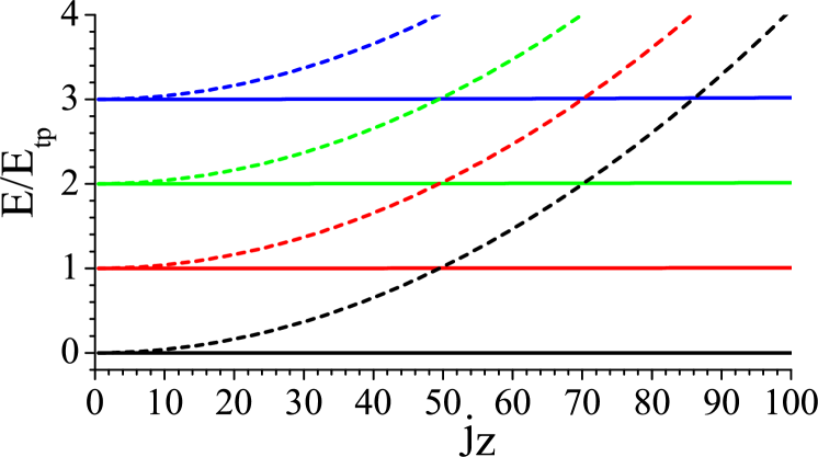
Figure 1: (Color online) Energy dispersions of the solutions for the first four LLs to the 2D reduced Hamiltonian Eq. (7) (solid lines), and those for (Eq. 1) (dashed lines). The value of $\alpha=l_{T}/l_{so}=35$. The lowest LLs of Eq. (7) are dispersionless with respect to $j_{z}$. Please note that the overall shift of the zero-point energy difference $\frac{1}{2}\hbar\omega$ is performed for the spectra of Eq. (1) for a better illustration.

The difference between the two Hamiltonians, Eq. (7) and (Eq. 1), is the $L_{z}\sigma_{z}$ term. Its effect depends on the distance $\rho$ from the center. We are interested in the case of $|z_{0}|\gg l_{T}$, i.e., $\alpha\gg 1$. Let us first consider the lowest LL. With small values of $j_{z}$, i.e., $m<\alpha$, $J_{m}(k_{0}\rho)$ and $J_{m+1}(k_{0}\rho)$ already decay before reaching the characteristic length $l_{T}$ of the Gaussian factor. We approximate their classic orbital radii as the locations of the maxima of Bessel functions, which are roughly $\rho_{c,j_{z}}\approx\frac{m}{\alpha}l_{T}<l_{T}$. In this regime, the effect of $L_{z}\sigma_{z}$ compared to the Rashba part is a small perturbation, of the order of $\omega\rho_{c,j_{z}}/\lambda=\rho_{c,j_{z}}/z_{0}\ll 1$. Thus, these two Hamiltonians share the same physics. On the other hand, let us consider the case of very large values of $j_{z}$, say, $m\gg\alpha^{2}$. The Bessel function behaves like $\rho^{m}$ or $\rho^{m+1}$ at $0<\rho<\frac{m}{\alpha}l_{T}$. The classic orbit radii are just $\rho_{c,j_{z}}\approx\sqrt{m}l_{T}$. The physics of Eq. (7) in this regime is dominated by the $L_{z}\sigma_{z}$ term and, thus, is the same as that of 2D quantum spin Hall LL wave functions. However, for Eq. (1), the projection to the sub-Hilbert space spanned by $\psi_{+}(\vec{k})$ is not valid. Its eigenstates in this regime cannot be viewed as LLs anymore. For intermediate values of $j_{z}$, i.e., $\alpha<m<\alpha^{2}$, the physics is a crossover between the above two limits.

For higher LLs of Eqs. (7) and (1), we expect that their wave functions can be approximated by a form of Eq. (13) by multiplying a polynomial of $\rho$ at the $n_{r}$-th power. As a result, the physics is similar to what is analyzed in the previous paragraph. At small values of $j_{z}<\alpha$, the energy gap is quantized in terms of the unit of $E_{tp}=\hbar\omega$ as in Eq. (4) for both Hamiltonians. At very large values of $j_{z}\gg\alpha^{2}$, the LLs of Eq. (7) become flat again and the quantization gap is at $2E_{tp}=2\hbar\omega$.

We perform the numerical calculation of the energy levels of the reduced 2D Hamiltonian Eq. (7), as plotted in Fig. 1. The numerically calculated spectra of Eq. 1, which were plotted in Refs. hu2011, and sinha2011, , are also presented for comparison. Only the spectra of $j_{z}>0$ are plotted, and those of $j_{z}<0$ are degenerate with their partners by the TR transformation which flips the sign of $j_{z}$. The lowest LL of Eq. (7) is flat as expected, while higher LLs are weakly dispersive which is hardly observable for the range of $j_{z}$ presented. The LLs of Eq. (1) are dispersive with the dependence on $j_{z}$ shown in Eq. (4). Inside the gaps between adjacent LLs of Eq. (1), the number of states is of the order of $\alpha$.

II.4 The Z₂ nature of the topological properties

Due to their connection to the 2D reduced version of the LL Hamiltonian, we still denote the low-energy bands of Eq. (1) as 2D parity breaking LLs. As shown in Eq. (4), although these LLs are not exactly flat, their dispersion over $j_{z}$ is strongly suppressed by the large value of $\alpha$. If the chemical potential $\mu$ lies in the middle of the band gap, the Fermi angular momentum $j_{kf,z}$ is at the order of $\alpha$. The classic radius of such a state is roughly $l_{T}$. As analyzed in Sec. II.2, for states with $|j_{z}|<\alpha$, two Hamiltonians Eqs. (1) and (7) share the same physics.

Compared to the usual 2D LL states, the SO coupled LLs of Eq. (1) in the form of Eq. (13) are markedly different. The smallest length scale is not $l_{T}$, but the SO coupling length scale $l_{so}=l_{T}/\alpha\ll l_{T}$. Instead, we can use $l_{T}$ as the cut-off of the sample size by imposing an open boundary condition at the radius of $l_{T}$. States with $|j_{z}|<\alpha$ are considered as bulk states which localize within the region of $\rho<l_{T}$. States with $|j_{z}|\sim\alpha$ are edge states.

We take the thermodynamic limit as follows. First, $\omega$ is fixed, which determines the LL gaps. Then we set $m\rightarrow 0$ and $\lambda\rightarrow\infty$ while keeping $l_{so}=\hbar/(m\lambda)$ unchanged, such that $l_{T}=\sqrt{\frac{\hbar}{m\omega}}\rightarrow\infty$. The number of bulk states scales linearly with $\alpha$, and the level spacing scales as $1/\alpha\rightarrow 0$ at the Fermi angular momentum $j_{k_{f},z}\sim\alpha$.

The next important question is the stability of the gapless edge modes. This situation is different from the usual 2D LL problem, in which inside each LL for each value of angular momentum $m$, there is only one state. Those edge modes are chiral and, thus, robust against external perturbations. Since Eq. (1) is TR symmetric, for each filled LL there is always a pair of degenerate edge modes $\psi_{n_{r},\pm j_{z}}$ on the Fermi energy, where $n_{r}$ is the LL index. Nevertheless, these two states are Kramer pairs under the TR transformation satisfying $T^{2}=-1$. In other words, the edge modes are helical rather than chiral.

We generalize the reasoning in Ref. kane2005, and kane2005a, for topological insulators with good quantum numbers of lattice momenta to our case with angular momentum good quantum numbers. Any TR-invariant perturbation cannot mix these two states to open a gap. In other words, the mixing term,

$$H_{mx}=g(\psi^{\dagger}_{2D,n_{r},j_{z}}\psi_{2D,n_{r},-j_{z}}+h.c.),$$ (21)

is forbidden by TR symmetry. On the other hand, if two LLs with indices $n_{r}$ and $n_{r}^{\prime}$ cut the Fermi energy, the mixing term,

$$H_{mx} = g^{\prime}(\psi^{\dagger}_{2D,n_{r},j_{z}}\psi_{2D,n^{\prime}_{r},-j_{z}}-\psi^{\dagger}_{2D,n^{\prime}_{r},j_{z}}\psi_{2D,n_{r},-j_{z}}$$ (22)

$$+ h.c.),$$

is allowed by TR symmetry and opens the gap. Consequently, the topological nature of such a system is characterized by the Z₂ index, even though it is not clear how to define the Pfaffian-like formula for it due to the lack of translational symmetry. kane2005a Similarly to the 2D topological insulators based on lattice Bloch-wave states, in our case, if odd numbers of LLs are filled such that there are odd numbers of helical edge modes, the gapless edge modes are robust.

Imagining an open boundary at $\rho\approx l_{T}$, we derive an effective edge Hamiltonian for these helical edge modes. As $|j_{z}|\sim\alpha$ and taking the limit of $\alpha\rightarrow+\infty$, these edge modes are pushed to the boundary. We expand the spectra around $j_{z,fm}$. The edge Hamiltonian in the basis of $j_{z}$ can be written as

$$H_{edge}=\sum_{j_{z}}(\frac{\hbar v_{f}}{l_{T}}|j_{z}|-\mu)\psi^{\dagger}_{n_{r},j_{z}}\psi_{n_{r},j_{z}}$$ (23)

where $\mu=\frac{\hbar v_{f}}{l_{T}}j_{z,fm}$. The edge modes $\psi_{n_{r},\pm j_{z}}$ around $j_{z,fm}$ can also be expanded as

$$\psi_{n_{r},j_{z}} = \left(\begin{array}[]{c}f_{n_{r}}e^{im\phi}\\ g_{n_{r}}e^{i(m+1)\phi}\end{array}\right),~{}~{}\psi_{n_{r},-j_{z}}=T\psi_{n_{r},j_{z}}.$$ (26)

$f_{n_{r}}$ and $g_{n_{r}}$ are real numbers parameterized as

$$f_{n_{r}}=\cos\frac{\theta_{n_{r}}}{2},\ \ \,g_{n_{r}}=\sin\frac{\theta_{n_{r}}}{2},$$ (27)

which are determined by the details of the edge. We neglect their dependence on $|j_{z}|$ for states close enough to the Fermi energy. The effective edge Hamiltonian can also be expressed in the plane-wave basis if we locally treat the edge as flat

$$H_{n_{r},edge} = v_{f}\Big{(}\sin\theta_{n_{r}}[(\vec{p}\times\hat{e}_{r})\cdot\hat{z})](\vec{\sigma}\cdot\hat{e}_{r})$$ (28)

$$+ \cos\theta_{n_{r}}(\vec{p}\times\hat{e}_{r})\cdot\sigma_{z}\Big{)}-\mu,$$

where $\hat{e}_{r}$ is the local normal direction on the circular edge; both terms are allowed by rotational symmetry, TR symmetry, and the vertical mirror symmetry in such a system. Each edge channel is a branch of helical one-dimensional Dirac fermion modes.

Equation (1) can be defined on the compact $S^{2}$ sphere, which takes the simple form

$$H=\frac{L^{2}}{2I}-\omega\vec{L}\cdot\vec{\sigma}.$$ (29)

The eigenvalues of $\vec{L}\cdot\vec{\sigma}$ take $l\hbar$ and $-(l+1)\hbar$ for the positive and negative helicities of $j_{\pm}=l\pm\frac{1}{2}$, respectively. For convenience, we choose the parameter value of $I\omega/\hbar$ as a large half-integer, then for the lower energy branch, the energy minimum takes place at $j_{0,+}=l_{0}+\frac{1}{2}=I\omega/\hbar$. The lowest LLs become SO-coupled harmonics with $j_{+}=j_{0,+}$ and ($2l_{0}+2$)-fold degeneracy. The gap between the lowest LLs and higher LLs is $\Delta=\hbar^{2}/(2I)$, which is independent of $\omega$. To take the thermodynamic limit, we keep $I$ constant while increasing the sphere radius $R$, and maintain $\omega$ scaling with $R^{2}$, such that the density of states on the sphere is a constant.

III Three-dimensional spin-orbit $\vec{\sigma}\cdot\vec{p}$ coupling in the harmonic trap

In this section, we generalize the results in Sec. II to three dimensions. We consider the $\vec{\sigma}\cdot\vec{p}$-type SO coupling combined with a 3D harmonic potential

$$H_{3D}=-\frac{\hbar^{2}\nabla^{2}}{2m}+\frac{1}{2}m\omega^{2}r^{2}-\lambda(-i\hbar\vec{\nabla}\cdot\vec{\sigma}).$$ (30)

Equation (30) possesses the 3D rotational symmetry, and TR symmetry of fermions with $T^{2}=-1$. The parity symmetry is broken by the $\vec{\sigma}\cdot\vec{k}$ term, and there is no mirror plane symmetry either. The quantities $l_{so}$, $l_{T}$, $\alpha$, and $k_{0}$ are defined in the same way as in Sec. II.

Although it is difficult to realize strong SO coupling in the form of $\sigma\cdot\vec{p}$ in solid-state systems, it can be designed through light-atom interactions in ultra cold atom systems. We present an experimental scheme to realize Eq. (30) in Sec. IV.

III.1 Energy spectra

Again, we consider the limit of strong SO coupling, i.e., $\alpha\gg 1$. It is straightforward to generalize the momentum space picture in Sec. II to the 3D case as presented in Ref. ghosh2011, and summarized below. The helicity operator $\vec{\sigma}\cdot\hat{k}$ is employed to define the helicity eigenstates of plane waves $(\vec{\sigma}\cdot\hat{k})\psi_{\vec{k},\pm}=\pm\psi_{\vec{k},\pm}$. Only positive-helicity states $\psi_{\vec{k}+}$ are kept in the low energy Hilbert space. The harmonic potential becomes the Laplacian operator in momentum space, and thus is equivalent to a quantum rotor subject to the Berry phase in momentum space as $V_{tp}=\frac{1}{2}m(i\vec{\nabla}_{k}-\vec{A}_{k})^{2}$. The moment of inertial is again $I=M_{k}k_{0}^{2}$ and $M_{k}=\hbar^{2}/(m\omega^{2})$. The Berry connection $\vec{A}_{k}=i\langle\psi_{\vec{k},\pm}|\vec{\nabla}_{k}|\psi_{\vec{k},\pm}\rangle$ is the vector potential of the U(1) magnetic monopole. As a result, the angular momentum quantization changes to that $j$ takes half-integer values starting from $\frac{1}{2}$. The energy dispersion becomes $E_{agl}(j)=\hbar^{2}j(j+1)/2I=(j(j+1)/2\alpha^{2})E_{tp}$, and each level is ($2j+1$)-fold degenerate. The radial quantization is the same as before. Thus the dispersion can be summarized as

$$E_{n_{r},j,j_{z}}\approx\Big{(}n_{r}+\frac{1}{2}-\frac{\alpha^{2}}{2}+\frac{j(j+1)}{2\alpha^{2}}\Big{)}E_{tp},$$ (31)

where $n_{r}$ is the band index, or, the LL index, and $j$ is the angular momentum quantum number.

III.2 Dimensional reduction from the 4D Landau level Hamiltonian

Following the same logic as in Sec. II.2, we present the dimensional reduction from the 4D LL Hamiltonian [Eq. (33)] to arrive at a 3D SO coupled Hamiltonian closely related to Eq. (30). The 3D LL Hamiltonian, Eq. (5), can be easily generalized to arbitrary dimensions by combining the $n$-D harmonic potential and the $n$-D SO coupling between orbital angular momenta and fermion spins in the fundamental spinor representations. li2011 In four dimensons, there are two non-equivalent fundamental spinors, both of which have two components. Without loss of generality, we choose one of them as

$$\sigma_{ij}=\epsilon_{ijk}\sigma_{k},\ \ \ \sigma_{i4}=\sigma_{i},$$ (32)

where $i,j=1,2$, and $3$. The orbital angular momentum operators are defined as $L_{ij}=-i\hbar x_{i}\nabla_{j}+i\hbar x_{j}\nabla_{i}$ where $i,j=1,2,3$, and $4$. The 4D LL Hamiltonian in the flat space is defined as

$$H_{4D,LL} = \sum_{i=1}^{4}-\frac{\hbar^{2}\nabla_{i}^{2}}{2m}+\frac{m\omega^{2}}{2}\sum_{i=1}^{4}r_{i}^{2}$$ (33)

$$- \omega\sum_{1\leq i<j\leq 4}L_{ij}\sigma_{ij},$$

which possesses TR and parity symmetry.

The $l$th-order 4D orbital spherical harmonics coupled to the fundamental spinor can be decomposed into the 4D SO-coupled spherical harmonics in the positive- and negative-helicity sectors, where $L_{ij}\sigma_{ij}$ take eigenvalues of $l\hbar$ and $-(l+2)\hbar$, respectively. The eigen wave functions of Eq. (33) in the positive-helicity channel are dispersionless with respect to $l$ as $E_{n_{r},+}=(2n_{r}+2)\hbar\omega$. Their radial wave functions are $R_{n_{r},l}(r)=r^{l}e^{-r^{2}/2l_{T}^{2}}F(-n_{r},l+2,r^{2}/l_{T}^{2})$, where $F$ is the standard confluent hypergeometric function. With an open boundary of an $S^{3}$ sphere, each filled LL contributes to a gapless surface mode of 3D Weyl fermions as

$$H_{3D,surface}=v_{f}\hat{e}_{r,i}\sigma_{ij}p_{j}-\mu,$$ (34)

where $\hat{e}_{r}$ is the unit vector normal to the $S^{3}$ sphere. The topological index for such a 4D LL systems with TR symmetry is $Z$ rather than $Z_{2}$.

We perform the dimensional reduction on Eq. (33) from four to three dimensions. We cut a 3D off-center hyper-plane perpendicular to the fourth axis with the interception $x_{4}=w_{0}$ Within this 3D hyper-plane of $(x_{1},x_{2},x_{3},x_{4}=w_{0})$, Eq. (33) reduces to

$$H_{3D,redc}=H_{3D,SO}-\omega\vec{L}\cdot\vec{\sigma},$$ (35)

where the first term is just Eq. (33) with the SO-coupling strength $\lambda=\omega w_{0}$. It contains another SO-coupling term, $\vec{L}\cdot\vec{\sigma}$, and its coefficient is the same as the harmonic trapping frequency. Similarly to the previous reduction from three to two dimensions, here we have $\alpha=l_{T}/l_{so}=|w_{0}|/l_{T}$. At $w_{0}=0$, Eq. (35) becomes the 3D LL Hamiltonian of Eq. (5) with parity symmetry. If $w_{0}\neq 0$, the $\vec{\sigma}\cdot\vec{p}$ term breaks parity symmetry. Following the same reasoning as in Sec. II.2, Eqs. (30) and (35) share the same physics for eigenstates with $j<\alpha$ in the case of $\alpha\gg 1$.

Similarly as before, we construct an off-center solution to the 4D LL problem. We use $\vec{r}$ to denote a point in the subspace of $x_{1,2,3}$, and $\hat{\Omega}$ as an arbitrary unit vector in the $x_{1}$-$x_{2}$-$x_{3}$ space. We consider the plane of $\hat{\Omega}$-$\hat{x}_{4}$ spanned by the orthogonal vectors $\hat{\Omega}$ and $\hat{x}_{4}$. It is easy to check that the following wave functions, which depends only on coordinates in the $\hat{\Omega}$-$\hat{x}_{4}$ plane are the lowest LL solutions to the 4D LL Hamiltonian, Eq. (33)

$$(\vec{r}\cdot\hat{\Omega}+ix_{4})^{l}e^{-\frac{r^{2}+x_{4}^{2}}{2l_{T}^{2}}}\otimes\alpha_{\hat{\Omega}},$$ (36)

where $\alpha_{\hat{\Omega}}=(\cos\frac{\theta}{2},\sin\frac{\theta}{2}e^{i\phi})^{T}$ satisfies

$$(\sigma_{i4}\Omega_{i})\alpha_{\hat{\Omega}}=(\vec{\sigma}\cdot\hat{\Omega})\alpha_{\hat{\Omega}}=\alpha_{\hat{\Omega}}.$$ (37)

In this set of wavefunctions, both the orbital angular momentum and spin are conserved and added up; they are called the highest weight states in group theory. In fact, these states can be rotated into any plane accompanied by a simultaneous rotation in the spin channel. Based on the structure of the highest weight states, we can still define the magnetic translation operator in the $\hat{\Omega}$-$x_{4}$ plane along the $x_{4}$ axis as

$$T_{\hat{\Omega}x_{4}}(w_{0}\hat{x}_{4})=\exp\Big{(}-w_{0}\partial_{x_{4}}-\frac{i}{l_{T}^{2}}(\vec{r}\cdot\Omega)w_{0}\Big{)}.$$ (38)

Applying this operator to the Gaussian pocket of the solution with $l=0$ in Eq. (36), we arrive at the off-center solution

$$\psi_{\Omega,w_{0}}(\vec{r},x_{4})=e^{-\frac{r^{2}+x_{4}^{2}}{2l_{T}^{2}}}e^{-i\frac{rw_{0}}{l_{T}^{2}}}\otimes\alpha_{\hat{\Omega}}.$$ (39)

This solution, however, breaks the rotational symmetry. In order to restore the 3D rotational symmetry around the new center $(0,0,0,w_{0})$, we perform a Fourier transformation over the direction of $\Omega$ as

$$\psi_{4D;j,j_{z}}(\vec{r},x_{4}) = \int d\Omega~{}{\cal Y}_{-\frac{1}{2},l+\frac{1}{2},m+\frac{1}{2}}(\hat{\Omega})\psi_{\Omega,w_{0}}(\vec{r},x_{4}).$$

where $j=l+\frac{1}{2}$ and $j_{z}=m+\frac{1}{2}$. Please note that due to the singularity of $\alpha_{\Omega}$ over the direction of $\hat{\Omega}$, monopole spherical harmonics, ${\cal Y}_{-\frac{1}{2},l+\frac{1}{2},m+\frac{1}{2}}(\Omega)$, are used instead of regular spherical harmonics.

Again, noting that $\partial_{x_{4}}\psi_{4D;j,j_{z}}(\vec{r},x_{4})|_{x_{4},w_{0}}=0$, we simply set $x_{4}=w_{0}$; then it is simple to check that the reduced 3D wave functions

$$\psi_{3D,j,j_{z}}(\vec{r})=\psi_{4D;j,j_{z}}(\vec{r},w_{0})$$ (41)

are the solutions to Eq. (35) for the lowest LLs as

$$H_{3D,redc}\psi_{3D,j,j_{z}}(\vec{r})=\Big{(}\frac{3}{2}-\frac{\alpha^{2}}{2}\Big{)}\hbar\omega\psi_{3D,j,j_{z}}(\vec{r}).$$

$\psi_{3D,j,j_{z}}(\vec{r})$ can be simplified as

$$\psi_{3D,jj_{z}}(\vec{r}) = e^{-\frac{r^{2}}{2l_{T}^{2}}}\Big{\{}j_{l}(k_{0}r)Y_{+,j,l,j_{z}}(\Omega_{r})+ij_{l+1}(k_{0}r)$$ (43)

$$\times Y_{-,j,l+1,j_{z}}(\Omega_{r})\Big{\}},$$

where $k_{0}=w_{0}/l_{T}^{2}=m\lambda/\hbar$ and $\lambda=w_{0}\omega$; $j_{l}$ is the $l$th-order spherical Bessel function. $Y_{\pm,j,l,j_{z}}$’s are the SO-coupled spherical harmonics defined as

$$Y_{+,j,l,j_{z}}(\Omega)=\Big{(}\sqrt{\frac{l+m+1}{2l+1}}Y_{lm},\sqrt{\frac{l-m}{2l+1}}Y_{l,m+1}\Big{)}^{T}$$

with a positive eigenvalue of $l\hbar$ for $\vec{\sigma}\cdot\vec{L}$, and

$$Y_{-,j,l,j_{z}}(\Omega)=\Big{(}-\sqrt{\frac{l-m}{2l+1}}Y_{lm},\sqrt{\frac{l+m+1}{2l+1}}Y_{l,m+1}\Big{)}^{T}$$

with a negative eigenvalue of $-(l+1)\hbar$ for $\vec{\sigma}\cdot\vec{L}$.

The difference between Eq. (35) and Eq. (30) is the term $\vec{\sigma}\cdot\vec{L}$, whose effect is weakened as the distance from center $r$ gets small. The radial distributions of $j_{l}(k_{0}r)$ in Eq. (43) and $J_{m}(k_{0}\rho)$ in Eq. (13) are similar. Following the same reasoning presented in Sec. II.2, in the limit of $\alpha\gg 1$, we can divide the lowest LL states of Eq. (43) into three regimes: $j<\alpha$, $j\gg\alpha^{2}$, and $\alpha<j<\alpha^{2}$. At $j<\alpha$, the classic orbit radius scales as $r_{c,j}\approx\frac{j}{\alpha}l_{T}<l_{T}$. Again in this regime, the effect of $\vec{\sigma}\cdot\vec{L}$ is a perturbation of the order of $r_{c,j_{z}}/z_{0}\ll 1$; thus the two Hamiltonians, Eq. (35) and Eq. (30), share the same physics. Similarly, in the regime of $j\gg\alpha^{2}$, $\vec{\sigma}\cdot\vec{L}$ dominates, and the physics of Eq. (35) comes back to the 3D LL Hamiltonian, Eq. (5), while that of Eq. (30) is no longer LL-like.

III.3 The Z₂ helical surface states

Following the same reasoning as in Sec. II.4, we denote the low-energy bands of Eq. (30) as 3D parity breaking LLs. For the lowest LL, below the energy of the bottom of the second LL, the angular momentum $j$ takes values from $\frac{1}{2}$ to the order of $\alpha$ at which the radius of the LL approaches $l_{T}$. For this regime $j<\alpha$, Eqs. (30) and (35) share the same physics. Again, the smallest length scale is the SO coupling length scale $l_{so}=l_{T}/\alpha\ll l_{T}$. States with $|j|\ll\alpha$ are considered bulk states which localize within the region $\rho\ll l_{T}$. States with $|j_{z}|\sim\alpha$ are edge states. The number of bulk states scales linearly with $\alpha^{2}$.

Now we impose an open boundary condition of an $S^{2}$ sphere with radius $r\approx l_{T}$, and consider the stability of the edge modes against TR invariant perturbations. Let us consider one filled LL. The Fermi energy lies between the gap, and thus cuts the dispersion at surface states. In the limit of $\alpha\rightarrow\infty$, the energy level spacing between adjacent angular momenta $j$ and $j+1$ scales as $\hbar\omega/\alpha\rightarrow 0$ for surface modes with $j\sim\alpha$. Thus we can always choose the Fermi angular momentum $j_{f}$ satisfying $j_{f}=2l+\frac{1}{2}$. For this value of $j_{f}$, there is an odd number of $2l+1$ Kramer pairs between $\psi_{j_{f},\pm j_{z}}$ for $j_{z}=\frac{1}{2}$ to $j_{f}$. Again according to the reasoning of the $Z_{2}$-classification in Refs. kane2005, and kane2005a, , these states cannot be fully gapped out by applying TR invariant perturbations. Certainly, for those states with $j=2l+\frac{3}{2}$ close to the Fermi energy, they can be fully gapped, but they are only part of the spectra, and do not change the topological properties. Again, if two LLs with different indices $n_{r}$ and $n_{r}^{\prime}$ cut the Fermi energy, the zero energy states at the Fermi level can be fully gapped out. Thus, the topological nature of Eq. (30) is $Z_{2}$.

We further present the effective surface Hamiltonian for surface modes in the limit of $j_{f}\sim\alpha\rightarrow+\infty$. The effective surface Hamiltonian of the 3D topological insulators with the spherical boundary condition has also been discussed in Refs. lee2009, and parente2011, . The surface Hamiltonian in the eigen-basis of $j$ and $j_{z}$ can be written as

$$H_{sf}=\sum_{j,j_{z}}(\frac{\hbar v_{f}}{l_{T}}|j|-\mu)\psi^{\dagger}_{n_{r},j,j_{z}}\psi_{n_{r},j,j_{z}},$$ (44)

where $\mu=\frac{\hbar v_{f}}{l_{T}}j_{f}$. The construction of the accurate surface Hamiltonian in the plane-wave basis depends on the detailed information of surface modes $\psi_{j,j_{z}}(r,\Omega_{r})$ for $j\approx j_{f}$ and, thus, is cumbersome. Nevertheless based on the symmetry analysis, we can write the general form as

$$H_{n_{r},edge} = v_{f}\Big{\{}\sin\theta_{n_{r}}(\vec{p}\times\vec{\sigma})\cdot\hat{e}_{r}$$ (45)

$$+ \cos\theta_{n_{r}}\big{[}\vec{p}\cdot\vec{\sigma}-(\vec{p}\cdot\hat{e}_{r})(\vec{\sigma}\cdot\hat{e}_{r})\big{]}\Big{\}}-\mu.$$

where $\hat{e}_{r}$ is the local norm direction on the $S^{2}$-sphere. Both terms obey the local $SO(2)$ rotational symmetry around the $\hat{e}_{r}$ and TR symmetry. The first Rashba term also obeys the vertical mirror symmetry, while the second term does not. The second term favors the spin aligning with the momentum, while the second favors a relative angle of 90^∘. For a general value of $\theta_{n_{r}}$, which is determined by the non-universal surface properties and $\theta_{n_{r}}$, Eq. (45) determines a relative rotation between spin and momentum orientation at the angle of $\theta_{n_{r}}$. It is still a helical Dirac Fermi surface.

IV Experimental realization for 3D SO coupling

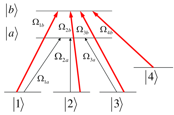
Figure 2: (Color online) Level diagram for atom-laser coupling. Four lower energy levels are coupled to two excited levels to compose a hybrid tripod and tetrapod configuration.

In the ultra cold atom context, there has been great progress in the synthetic gauge field, or, artificial SO coupling from light-atom interactions dalibard2011 . Experimentally, artificial SO coupling has been generate in ultra cold atom systems. lin2011 Two dimensional Rashba and Dresselhaus SO coupling in the harmonic potential has been proposed using a double-tripod configuration. juzeliunas2011 Since the pseudo-spin degrees of freedom are represented by the two lowest energy levels, this scheme is immune to decay due to collision and spontaneous emission process. ruseckas2005

In this section, we propose the experimental realization for the 3D SO coupling of the $\vec{\sigma}\cdot\vec{p}$ type in Eq. (30). Here we generalize the scheme in Ref. juzeliunas2011, to a combined tripod and tetrapod level configuration as depicted in Fig. 2. Three internal levels $|1\rangle$, $|2\rangle$, and $|3\rangle$ couple the excited state $|a\rangle$ to form a tripod configuration. A tetrapod-like coupling is formed by coupling the four levels $|1\rangle-|4\rangle$ to the common excited state $|b\rangle$. The single-particle Hamiltonian reads

$$H=\frac{p^{2}}{2m}+\frac{1}{2}m\omega^{2}r^{2}+H_{al},$$ (46)

where $m$ is the mass of the atom; $H_{al}$ represents the atom-laser coupling. In the interaction picture, $H_{al}$ can be written under the rotating wave approximation as

$$H_{al} = -\hbar\sum_{m=a,b}\big{\{}\Omega_{1m}|m\rangle\langle 1|+\Omega_{2m}|m\rangle\langle 2|+\Omega_{3m}|m\rangle\langle 3|$$ (47)

$$+ h.c.\big{\}}-\hbar\left[\Omega_{4b}|b\rangle\langle 4|+h.c.\right],$$

where $\Omega_{im}$ are the corresponding Rabi frequencies between the internal states $|i\rangle$ and $|m\rangle$ with $m=a,b$ .

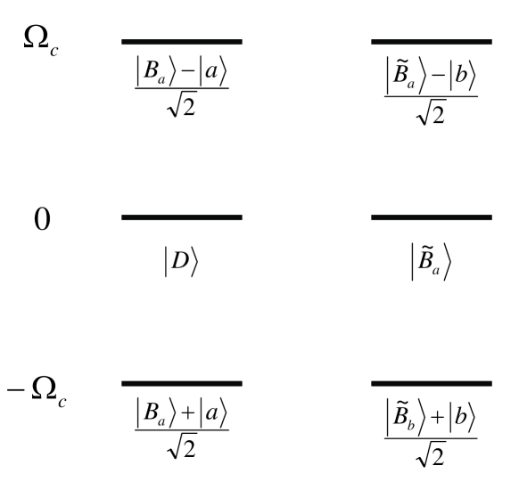
Figure 3: Energy levels of the atom-laser coupling Hamiltonian Eq. 51.

We introduce the following two bright states

$$|B_{m}\rangle=(\Omega_{1m}^{*}|1\rangle+\Omega_{2m}^{*}|2\rangle+\Omega_{3m}^{*}|3\rangle)/\Omega_{m},$$ (48)

where $m=a,b$ and $\Omega_{m}=\sqrt{|\Omega_{1m}|^{2}+|\Omega_{2m}|^{2}+|\Omega_{3m}|^{2}}$. The atom-laser coupling can be rewritten as

$$H_{al} = -\hbar\Big{\{}\Omega_{a}|a\rangle\langle B_{a}|+\emph{h.c.}\Big{\}}$$ (49)

$$- \hbar\Big{\{}\Omega_{b}|b\rangle\langle B_{b}|+\Omega_{4b}|b\rangle\langle 4|+h.c.\Big{\}}.$$

To further simplify the model, here we assume $\langle B_{a}|B_{b}\rangle=0$, which can be achieved by choosing

$$\Omega_{jm} = \frac{\Omega_{m}}{\sqrt{3}}e^{i(\vec{k}_{j}\cdot\vec{r}+\theta_{jm})},\ \ \,(j=1,2,3;m=a,b)$$ (50)

with $\theta_{ja}=(j-2)2\pi/3$ and $\theta_{jb}=-(j-2)2\pi/3$. We also choose $\Omega_{4b}=\Omega_{4}e^{i(\vec{k}_{4}\cdot\vec{r}+\theta_{4})}$, and set $\Omega_{c}=\Omega_{a}$, $\Omega_{b}=\Omega_{c}\cos\phi$, and $\Omega_{4}=\Omega_{c}\sin\phi$. Using these notations, $H_{al}$ is simplified as

$$H_{al}=-\hbar\left[\Omega_{c}(|a\rangle\langle B_{a}|+|b\rangle\langle\tilde{B}_{b}|)+\emph{h.c.}\right],$$ (51)

where $|\tilde{B}_{b}\rangle=\cos\phi|B_{b}\rangle+\sin\phi|\tilde{4}\rangle$ and $|\tilde{4}\rangle=e^{-i(\vec{k}_{4}\cdot\vec{r}+\theta_{4})}|4\rangle$. The above Hamiltonian supports three pairs of degenerated eigenstates with energy difference $\hbar|\Omega_{c}|$, as depicted in Fig. (3). Explicitly, the eigen-vectors are written as

$$|G_{1}\rangle = \frac{|B_{a}\rangle+|a\rangle}{\sqrt{2}},\ \ \,|G_{2}\rangle=\frac{|\tilde{B}_{b}\rangle+|b\rangle}{\sqrt{2}},$$

$$|G_{3}\rangle = |D\rangle,\ \ \,\ \ \,\ \ \,\ \ \,|G_{4}\rangle=|\tilde{B}^{\perp}_{b}\rangle,$$

$$|G_{5}\rangle = \frac{|B_{a}\rangle-|a\rangle}{\sqrt{2}},\ \ \,|G_{6}\rangle=\frac{|\tilde{B}_{b}\rangle+|b\rangle}{\sqrt{2}},$$ (52)

where $|D\rangle=\sum_{j}e^{-i\vec{k}_{j}\cdot\vec{r}}|j\rangle/\sqrt{3}$ and $|\tilde{B}^{\perp}_{b}\rangle=\sin\phi|B_{b}\rangle-\cos\phi|\tilde{4}\rangle$. Therefore, the two degenerate ground states can be used as pseudo-spin $1/2$ degrees of freedom.

If the trapping frequency satisfies $\omega\ll|\Omega_{c}|$, according to the adiabatic approximation, we neglect the coupling between the ground-state manifold and other states. Therefore, atoms in the subspace spanned by $|G_{1}\rangle$ and $|G_{2}\rangle$ evolve according to the effective Hamiltonian

$$H_{e}=\frac{(\vec{p}-\vec{A})^{2}}{2m}+\frac{1}{2}m\omega^{2}r^{2}+\Phi,$$ (53)

where the non-Abelian gauge potential $\vec{A}$ is a $2\times 2$ matrix with the elements

$$\vec{A}_{ij}=i\hbar\langle G_{i}|\vec{\nabla}|G_{j}\rangle,$$ (54)

where $i,j=1,2$; $\Phi$ is a scalar potential induced by the coupling laser beams.

An isotropic $3$D $\vec{\sigma}\cdot\vec{p}$-like SO coupling can be obtained by a 3D set-up of laser configurations as

$$\vec{k}_{1} = \kappa(-\frac{1}{2},-\frac{\sqrt{3}}{2},0),\ \ \,\vec{k}_{2}=\kappa(0,1,0),$$

$$\vec{k}_{3} = \kappa(-\frac{1}{2},\frac{\sqrt{3}}{2},0),\ \ \,\vec{k}_{4}=\kappa(0,0,-\sqrt{\frac{7+\sqrt{17}}{8}}).$$ (55)

In this case, the corresponding vector and scale potential are calculated as

$$\frac{\vec{A}}{\hbar} = 0.166\kappa\left[\sigma_{x}\vec{e}_{x}+\sigma_{y}\vec{e}_{y}+(\sigma_{z}-I)\vec{e}_{z}\right],$$

$$\Phi = 0.445\frac{\hbar^{2}\kappa^{2}}{2m}\hat{I}.$$ (56)

The $\Phi$ term is a constant and, thus, can be dropped off. The Abelian part in the gauge potential $A_{z}$ is a constant, which can be absorbed by a gauge transformation. Consequently, the remaining constant non-Abelian gauge potential behaves as a $\vec{\sigma}\cdot\vec{p}$ type SO coupling.

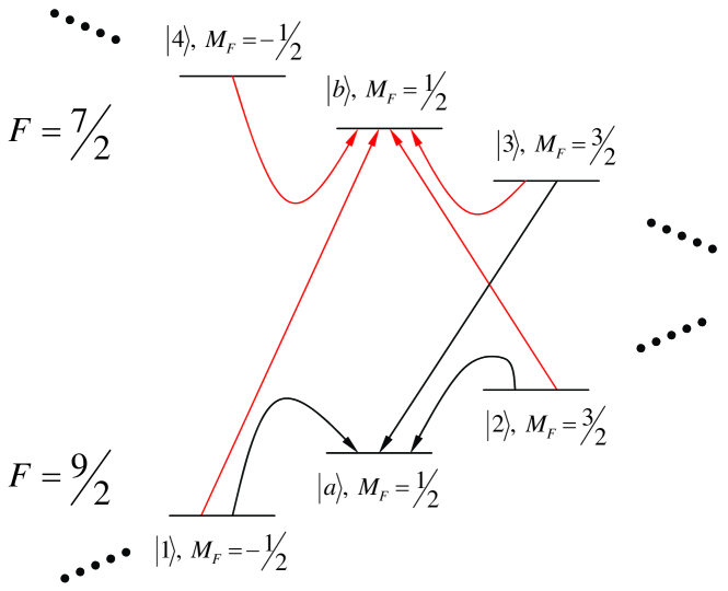
Figure 4: (Color online) Energy level scheme for alkali atoms ${}^{40}K$. The Zeeman sublevels of two hyperfine states $F=\frac{9}{2}$ and $F=\frac{7}{2}$ can be used to fulfill our requirements. Lines or curves with an arrow indicate effective transitions between different magnetic levels which can be implemented using resonant Raman processes. Other levels, which are not involved in the scheme, are not shown.

The above-considered level structure can be found for example, in alkali atoms with large spins. Figure 4 shows the hyperfine ground state manifolds of ${}^{2}S_{1/2}$ for ${}^{40}K$ atoms under an external magnetic field. The energy levels $|1\rangle\sim|4\rangle$, $|a\rangle$, and $|b\rangle$ can be selected as different Zeeman sublevels of $F=\frac{9}{2}$ and $F=\frac{7}{2}$. Using the notation of $|FM_{F}\rangle$ to denote each state, we choose $|1\rangle=|\frac{9}{2},-\frac{1}{2}\rangle$, $|2\rangle=|\frac{9}{2},\frac{3}{2}\rangle$, $|3\rangle=|\frac{7}{2},\frac{3}{2}\rangle$, $|4\rangle=|\frac{7}{2},-\frac{1}{2}\rangle$, $|a\rangle=|\frac{9}{2},\frac{1}{2}\rangle$ and $|b\rangle=|\frac{7}{2},\frac{1}{2}\rangle$. The coupling between different levels is achieved for example, by using two laser beams under second-order resonant Raman process. The two lasers can be chosen to be circularly polarized and $\pi$ polarized, respectively, in order to satisfy the selection rule. Finally, wave vectors of individual laser beams can also be adjusted so that Eq. (56) is fulfilled.

V Conclusion and outlook

We have studied rotationally and TR symmetric LL systems in both 2D and 3D systems with breaking parity symmetry, whose topological properties are characterized by the $Z_{2}$ class. These Hamiltonians are simply 2D harmonic potentials plus Rashba SO coupling, or 3D harmonic potentials plus $\vec{\sigma}\cdot\vec{p}$-type SO coupling with a strong SO coupling strength. For low-energy bands, the dispersions over angular momenta are strongly suppressed by SO coupling, to be nearly flat. Up to a small difference which can be treated perturbatively, these Hamiltonians can be systematically investigated through dimensional reduction on the high-dimensional LL problems by cutting an off-center plane in the 3D LL Hamiltonian or an off-center hyper plane in the 4D LL Hamiltonian. The parity breaking LL wavefunctions in two and three dimensions are presented explicitly. With open boundary conditions, helical edge states are found in two dimensions, and surface states are found in three dimensions. These states can be realized in ultra cold atom systems in a harmonic trap combined with synthetic gauge fields, i.e., artificial SO coupling. In particular, we propose an experimental scheme to realize the 3D Hamiltonian.

The above dimensional procedure can be straightforwardly generalized to arbitrary dimensions based on our previous construction of high dimensional LL Hamiltonians, li2011 and so can the general parity breaking LL wavefunctions in $N$ dimensions. The nice analytical properties of the 2D and 3D LL wave functions breaking parity symmetry also provide a good opportunity to further construct many-body wave functions of the factional topological states. These properties will be investigated in a future publication.

- (1) M. Hasan and C. Kane, Rev. Mod. Phys. 82, 3045 (2010).
- (2) X.-L. Qi and S.-C. Zhang, Rev. Mod. Phys. 83, 1057–1110 (2011).
- (3) D. J. Thouless, M. Kohmoto, M. P. Nightingale, and M. den Nijs, Phys. Rev. Lett. 49, 405 (1982).
- (4) M. Kohmoto, Ann. Phys. 160, 343 (1985).
- (5) F. D. M. Haldane, Phys. Rev. Lett. 61, 2015 (1988).
- (6) C. L. Kane and E. J. Mele, Phys. Rev. Lett. 95, 146802 (2005).
- (7) C. L. Kane and E. J. Mele, Phys. Rev. Lett. 95, 226801 (2005).
- (8) B. A. Bernevig and S. C. Zhang, Phys. Rev. Lett. 96, 106802 (2006).
- (9) B. Bernevig, T. Hughes, and S. Zhang, Science 314, 1757 (2006).
- (10) L. Fu and C. L. Kane, Phys. Rev. B 76, 045302 (2007).
- (11) L. Fu, C. L. Kane, and E. J. Mele, Phys. Rev. Lett. 98, 106803 (2007).
- (12) J. E. Moore and L. Balents, Phys. Rev. B 75, 121306 (2007).
- (13) X.-L. Qi, T. L. Hughes, and S.-C. Zhang, Phys. Rev. B 78, 195424 (2008).
- (14) R. Roy, New J. Phys. 12, 065009 (2010).
- (15) D. Hsieh et al., Nature 452, 970 (2008).
- (16) M. König et al., Science 318, 766 (2007).
- (17) H. Zhang et al., Nature Phys. 5, 438 (2009).
- (18) D. Hsieh et al., Phys. Rev. Lett. 103, 146401 (2009).
- (19) Y. Xia et al., Nature Phys. 5, 398 (2009).
- (20) M. Zahid Hasan, J. E. Moore, Ann. Rev. Cond. Matt. Phys., 2, 55 (2011).
- (21) S. Ryu, A. Schnyder, A. Furusaki, A. Ludwig, New J. Phys. 12, 065010 (2010).
- (22) A. Kitaev, American Institute of Physics Conference Series, Vol. 1134, 22 (2009).
- (23) S. C. Zhang and J. Hu, Science 294, 823 (2001).
- (24) D. Karabali and V. P. Nair, Nucl. Phys. B 641, 533 (2002).
- (25) H. Elvang and J. Polchinski, Comptes Rendus Physique 4, 405 (2003).
- (26) B. A. Bernevig, J. Hu, N. Toumbas, and S.-C. Zhang, Phys. Rev. Lett. 91, 236803 (2003).
- (27) K. Hasebe, Symmetry, Integrability and Geometry: Methods and Applications 6, (2010).
- (28) M. Fabinger, JHEP 2002, 037 (2002).
- (29) Y. Li and C. Wu, ArXiv:1103.5422 (2011).
- (30) Y. Li, K. Intriligator, Y. Yu, C. Wu, Phys. Rev. B 85, 085132 (2012).
- (31) A. J. Niemi and G. W. Semenoff, Phys. Rev. Lett. 51, 2077 (1983).
- (32) R. Jackiw, Phys. Rev. D 29, 2375 (1984).
- (33) A. N. Redlich, Phys. Rev. D 29, 2366 (1984).
- (34) G. W. Semenoff, Phys. Rev. Lett. 53, 2449 (1984).
- (35) K. S. Novoselov et al., Nature (London)438, 197 (2005).
- (36) Y. Zhang, Y.-W. Tan, H. L. Stormer, and P. Kim, Nature (London)438, 201 (2005).
- (37) A. H. Castro Neto et al., Rev. Mod. Phys. 81, 109 (2009).
- (38) E. I. Rashba, Sov. Phys. Solid State 2, 1109 (1960).
- (39) C. R. Ast, J. Henk, A. Ernst, L. Moreschini, M. C. Falub, D. Pacile, P. Bruno, K. Kern, and M. Grioni, Phys. Rev. Lett. 98, 186807 (2007).
- (40) E. Berg, M. S. Rudner, and S. A. Kivelson, Phys. Rev. B 85 035116, (2012).
- (41) C. Wu, I. Mondragon-Shem, arXiv:0809.3532v1.
- (42) C. Wu, I. Mondragon-Shem, X. F. Zhou, Chin. Phys. Lett. 28, 097102 (2011).
- (43) Y.-J. Lin, K. Jimenez-Garcia, I. B. Spielman, Nature 471, 83-86 (2011).
- (44) C. Wang, C. Gao, C. M. Jian, and H. Zhai, Phys. Rev. Lett. 105, 160403 (2010).
- (45) Tin-Lun Ho, Shizhong Zhang, Phys. Rev. Lett. 107, 150403 (2011).
- (46) S. K. Ghosh, J. P. Vyasanakere, and V. B. Shenoy, Phys. Rev. A 84 053629, (2011).
- (47) H. Hu, B. Ramachandhran, H. Pu, X. J. Liu, Phys. Rev. Lett. 108 010402, (2012).
- (48) S. Sinha, R. Nath, L. Santos, arXiv:1109.2045.
- (49) Xiang-Fa Zhou, Jing Zhou, Congjun Wu, Phys. Rev. A 84, 063624 (2011).
- (50) D. Xiao, M. C. Chang, Q. Niu, Rev. Mod. Phys. 82, 1959 (2010).
- (51) D. H. Lee, Phys. Rev. Lett. 103, 196804 (2009).
- (52) V.Parente, P.Lucignano, P.Vitale, A.Tagliacozzo, F.Guinea, Phys. Rev.B 83 075424, (2011).
- (53) J. Dalibard, F. Gerbier, G. Juzeliūnas, P. Oehberg, Rev. Mod. Phys. 83, 1523 (2011).
- (54) G. Juzeliunas, J. Ruseckas, D. L. Campbell, I. B. Spielman, Proc. SPIE 7950, 79500M (2011).
- (55) J. Ruseckas, G. Juzeliunas, P. Ohberg, and M. Fleischhauer, Phys. Rev. Lett. 95, 010404 (2005).