Abstract

In this article, we study the light-flavor scalar and axial-vector diquark states in the vacuum and in the nuclear matter using the QCD sum rules in an systematic way, and make reasonable predictions for their masses in the vacuum and in the nuclear matter.

PACS numbers: 12.38.Lg; 12.39.Ki

Key Words: Diquark states, QCD sum rules

1 Introduction

We can rephrase the scattering amplitude of one-gluon exchange into an antisymmetric antitriplet $\overline{\bf{3}}_{c}$ and an symmetric sextet $\bf{6}_{c}$ in the color-space,

$$\left(\frac{\lambda^{a}}{2}\right)_{ki}\left(\frac{\lambda^{a}}{2}\right)_{lj} = -\frac{1}{3}(\delta_{jk}\delta_{il}-\delta_{ik}\delta_{jl})+\frac{1}{6}(\delta_{jk}\delta_{il}+\delta_{ik}\delta_{jl})\,,$$ (1)

where the $\lambda^{a}$ is the Gell-Mann matrix element, and the $i,j$ and $k,l$ are the color indexes of the incoming and outgoing quarks respectively. The attractive interaction in the antisymmetric antitriplet favors the formation of the diquark states in the color antitriplet, while the most stable diquark states maybe exist in the color antitriplet $\overline{\bf{3}}_{c}$, flavor antitriplet $\overline{\bf{3}}_{f}$ and spin singlet ${\bf{1}}_{s}$ channels due to Fermi-Dirac statistics [1]. We can take the diquarks as basic constituents to obtain a new spectroscopy for the mesons and baryons [2, 3], and the diquark states play an important role in many phenomenological analysis [4, 5]. For example, we usually take the nonet scalar mesons below $1\,\rm{GeV}$ as the tetraquark states consist of the scalar diquark states $[qq]_{\overline{\bf{3}}_{c}}$ and $[\bar{q}\bar{q}]_{\bf{3}_{c}}$ in the relative $S$-wave [5], and study the octet and decuplet baryons as the quark-diquark bound states [6].

The QCD sum rules is a powerful theoretical tool in studying both the in-vacuum and in-medium hadronic properties [7], and has been applied extensively to study the properties of the in-vacuum hadrons and the in-medium light-flavor hadrons and charmonium states [8, 9, 10]. In the limit $m_{u}=m_{d}\rightarrow 0$, the in-medium nucleon mass $M_{N}^{*}$ can be related with the in-medium quark condensate $\langle\bar{q}q\rangle_{\rho_{N}}$ through the simple relation $M_{N}^{*}=-\frac{8\pi^{2}}{T^{2}}\langle\bar{q}q\rangle_{\rho_{N}}$, where the $T^{2}$ is the Borel parameter. It is interesting to study the diquark states in the nuclear matter, as they are basic constituents of the baryons and play an important role in understanding the strong interactions and the relativistic heavy ion collisions. The in-medium baryon properties will be studies by the CBM (compressed baryonic matter) and $\rm{\bar{P}ANDA}$ collaborations unto the charm sector at the upcoming FAIR (facility for antiproton and ion research) project at GSI (heavy ion research lab) [11, 12]. The in-vacuum light and heavy scalar and axial-vector diquark states have been studies with the QCD sum rules [13, 14, 15], we extend the previous works to study the in-medium mass modifications of the light-flavor diquark states.

The article is arranged as follows: we derive the QCD sum rules for the light-flavor scalar and axial-vector diquark states in the vacuum and in the nuclear matter in Sect.2; in Sect.3, we present the numerical results and discussions; and Sect.4 is reserved for our conclusions.

2 The scalar and axial-vector diquark states with QCD Sum Rules

We write down the two-point correlation functions $\Pi(p)$ and $\Pi_{\mu\nu}(p)$ in the nuclear matter,

$$\Pi(q) = i\int d^{4}xe^{iqx}\langle\Psi_{0}|T\{J(x)J^{\dagger}(0)\}|\Psi_{0}\rangle\,,$$

$$\Pi_{\mu\nu}(q) = i\int d^{4}xe^{iqx}\langle\Psi_{0}|T\{J_{\mu}(x)J_{\nu}^{\dagger}(0)\}|\Psi_{0}\rangle\,,$$ (2)

where $J(x)=J^{a}(x),\eta^{a}(x)$ and $J_{\mu}(x)=J_{\mu}^{a}(x),\eta_{\mu}^{a}(x)$,

$$J^{a}(x) = \epsilon^{abc}u_{b}^{T}(x)C\gamma_{5}d_{c}(x)\,,$$

$$\eta^{a}(x) = \epsilon^{abc}q_{b}^{T}(x)C\gamma_{5}s_{c}(x)\,,$$

$$J^{a}_{\mu}(x) = \epsilon^{abc}u_{b}^{T}(x)C\gamma_{\mu}d_{c}(x)\,,$$

$$\eta^{a}_{\mu}(x) = \epsilon^{abc}q_{b}^{T}(x)C\gamma_{\mu}s_{c}(x)\,,$$ (3)

the currents $J(x)$ and $J_{\mu}(x)$ interpolate the scalar and axial-vector diquark states, respectively, the $a$, $b$, $c$ are the color indexes, the $C$ is the charge conjunction matrix, and the $|\Psi_{0}\rangle$ is the nuclear matter ground state.

In the limit $|\Psi_{0}\rangle\to|0\rangle$, we insert a complete set of intermediate ”hadronic” states with the same quantum numbers as the current operators $J(x)$ and $J_{\mu}(x)$ into the correlation functions $\Pi(p)$ and $\Pi_{\mu\nu}(p)$ to obtain the ”hadronic” representation [7], then isolate the ground state contributions from the scalar and axial-vector diquarks, and obtain the results:

$$\Pi(q) = \frac{f_{S}^{2}}{M_{S}^{2}-q^{2}}+\cdots\,,$$

$$\Pi_{\mu\nu}(q) = \frac{f_{A}^{2}}{M_{A}^{2}-q^{2}}\left(-g_{\mu\nu}+\frac{q_{\mu}q_{\nu}}{q^{2}}\right)+\cdots\,,$$ (4)

$$= \Pi(q)\left(-g_{\mu\nu}+\frac{p_{\mu}p_{\nu}}{q^{2}}\right)+\cdots\,,$$

where the pole residues $f_{S}$ and $f_{A}$ are defined as $\langle 0|J(0)|S(q)\rangle=f_{S}$ and $\langle 0|J_{\mu}(0)|A(q)\rangle=f_{A}\epsilon_{\mu}$, the $\epsilon_{\mu}$ is the polarization vector.

Here we will take a short digression to discuss the application of the QCD sum rules in studying the diquark states. In the QCD sum rules, we perform the operator product expansion at not so deep Euclidean space, where the approximation of the correlation functions by perturbative terms plus some nonperturbative terms makes sense and the contributions from the condensates (or nonperturbative terms) are sizeable. There are significant differences between the correlation functions of current operators interpolating the diquarks and conventional handrons, we can continue the hadronic correlation functions to the physical region for the conventional hadrons, but not for the diquarks, as the diquarks are non-asymptotic states, there are significant differences between the diquark states and conventional hadrons. The one-gluon exchange results in strong attractions in the color antitriplet channel $\bar{\bf{3}}_{c}$, the quark-quark system maybe form quasibound states or loosely bound states (diquark states), which are characterized by the correlation length $\mathbb{L}$. At the distance $l>\mathbb{L}$, the $\bar{\bf{3}}_{c}$ diquark state combines with one quark or one $\bf{3}_{c}$ antidiquark to form a baryon state or a tetraquark state, while at the distance $l<\mathbb{L}$, the $\bar{\bf{3}}_{c}$ diquark states dissociate into asymptotic quarks and gluons gradually. We can take the diquark state $\mathbb{D}$ as an effective colored hadron and the diquark mass as an effective quantity, $M_{\mathbb{D}}\sim\frac{1}{\mathbb{L}}$, the correlation functions can be continued to the physical region, where the quark-quark correlations exist. The transitions two-quarks $\leftrightarrow$ diquarks $\leftrightarrow$ hadrons are not abrupt, the typical correlation lengths $\mathbb{L}$ have uncertainties, we have the freedom to choose somewhat larger or smaller diquark masses in model-buildings. The correlation functions are approximated by a pole term plus a perturbative continuum.

We use the dispersion relation to express the invariant functions $\Pi(q_{0},\vec{q})$ in the following form:

$$\Pi(q_{0},\vec{q}) = {1\over 2\pi i}\int_{-\infty}^{\infty}~{}d\omega{\Delta\Pi(\omega,\vec{q})\over\omega-q_{0}}\,,$$

$$\Delta\Pi(\omega,\vec{q}) = {\rm{limit}}_{\epsilon\to 0}\left[\Pi(\omega+i\epsilon,\vec{q})-\Pi(\omega-i\epsilon,\vec{q})\right]\,.$$ (5)

In the nuclear matter, the corresponding imaginary parts of the spectral densities can be expressed as

$$\Delta\Pi(\omega,\vec{q})=i\pi\left[F_{+}\delta(q_{0}-M_{+})-F_{-}\delta(q_{0}+M_{-})\right]\,,$$ (6)

where the $F_{\pm}$ and $M_{\pm}$ are the pole residues and masses, respectively. In the vacuum limit, $F_{\pm}=\frac{f_{S}^{2}}{M_{S}},\frac{f_{A}^{2}}{M_{A}}$ and $M_{\pm}=M_{S},M_{A}$. Thereafter we will use the same notations for the masses and pole residues both in the vacuum and in the nuclear matter for simplicity.

We carry out the operator product expansion in the finite nuclear density at large spacelike region $q^{2}\ll 0$, and express the invariant functions $\Pi(q_{0},\vec{q})$ at the level of quark-gluon degrees of freedom as [9, 10],

$$\Pi(q_{0},\vec{q}) = \sum_{n}C_{n}(q_{0},\vec{q})\langle{O}_{n}\rangle_{\rho_{N}}\,,$$ (7)

where the $C_{n}(q_{0},\vec{q})$ are the Wilson coefficients, the in-medium condensates $\langle{O}_{n}\rangle_{\rho_{N}}=\langle\Psi_{0}|{O}_{n}|\Psi_{0}\rangle=\langle{\cal{O}}\rangle+\rho_{N}\langle{\cal{O}}\rangle_{N}$ at the low nuclear density, the $\langle{\cal{O}}\rangle$ and $\langle{\cal{O}}\rangle_{N}$ denote the vacuum condensates and nuclear matter induced condensates, respectively, then take the limit $u_{\mu}=(1,0)$, $q_{0}^{2}=q^{2}$, and obtain the imaginary parts of the QCD spectral densities according to Eq.(5). One can consult Refs.[9, 10] for the technical details in the operator product expansion. In calculations, we consult the QCD sum rules for the light-flavor scalar and axial-vector diquark states in the vacuum, and take the analytical expressions of the perturbative terms and the dimension-6 terms from Ref.[13].

We can match the phenomenological side with the QCD side of the spectral densities, and multiply both sides with the weight function $\omega e^{-\frac{\omega^{2}}{T^{2}}}$, then perform the integral $\int_{-\omega_{0}}^{\omega_{0}}d\omega$,

$$\int_{-\omega_{0}}^{\omega_{0}}d\omega\Delta\Pi(\omega,\vec{q})\omega e^{-\frac{\omega^{2}}{T^{2}}}\,,$$ (8)

where the $\omega_{0}$ is the threshold parameter, finally obtain the following two QCD sum rules in the nuclear matter:

$$f_{S}^{2}e^{-\frac{M_{S}^{2}}{T^{2}}} = \frac{3T^{4}}{4\pi^{2}}\left[\frac{\alpha_{s}(T)}{\alpha_{s}(\mu)}\right]^{\frac{4}{9}}\left\{\left(1+\frac{17\alpha_{s}(T)}{6\pi}\right)\left[1-\left(1-\frac{s_{0}}{T^{2}}\right)e^{-\frac{s_{0}}{T^{2}}}\right]\right.$$ (9)

$$\left.-\frac{\alpha_{s}(T)}{\pi}\int_{0}^{\frac{s_{0}}{T2}}dxe^{-x}x{\rm log}x-\frac{2m_{s}^{2}}{T^{2}}\left(1-e^{-\frac{s_{0}}{T^{2}}}\right)\right\}-4\langle q^{\dagger}iD_{0}q\rangle_{\rho_{N}}-4\langle s^{\dagger}iD_{0}s\rangle_{\rho_{N}}$$

$$-2m_{s}\langle\bar{q}q\rangle_{\rho_{N}}+2m_{s}\langle\bar{s}s\rangle_{\rho_{N}}+\frac{m_{s}\langle\bar{q}g_{s}\sigma Gq\rangle_{\rho_{N}}}{T^{2}}+\frac{8m_{s}\langle\bar{q}iD_{0}iD_{0}\rangle_{\rho_{N}}}{T^{2}}$$

$$+\frac{1}{8}\langle\frac{\alpha_{s}GG}{\pi}\rangle_{\rho_{N}}+\frac{8\pi\alpha_{s}\langle\bar{q}q\rangle\langle\bar{s}s\rangle_{\rho_{N}}}{T^{2}}-\frac{16\pi\alpha_{s}\left[\langle\bar{q}q\rangle_{\rho_{N}}^{2}+\langle\bar{s}s\rangle_{\rho_{N}}^{2}\right]}{27T^{2}}\,,$$

$$f_{A}^{2}e^{-\frac{M_{A}^{2}}{T^{2}}} = \frac{T^{4}}{2\pi^{2}}\left[\frac{\alpha_{s}(T)}{\alpha_{s}(\mu)}\right]^{\frac{4}{9}}\left\{\left(1+\frac{\alpha_{s}(T)}{2\pi}\right)\left[1-\left(1-\frac{s_{0}}{T^{2}}\right)e^{-\frac{s_{0}}{T^{2}}}\right]-\frac{3m_{s}^{2}}{2T^{2}}\left(1-e^{-\frac{s_{0}}{T^{2}}}\right)\right\}$$ (10)

$$-\frac{8\langle q^{\dagger}iD_{0}q\rangle_{\rho_{N}}}{3}-\frac{8\langle s^{\dagger}iD_{0}s\rangle_{\rho_{N}}}{3}-2m_{s}\langle\bar{q}q\rangle_{\rho_{N}}+\frac{2m_{s}\langle\bar{s}s\rangle_{\rho_{N}}}{3}$$

$$+\frac{m_{s}\langle\bar{q}g_{s}\sigma Gq\rangle_{\rho_{N}}}{T^{2}}+\frac{8m_{s}\langle\bar{q}iD_{0}iD_{0}\rangle_{\rho_{N}}}{T^{2}}-\frac{1}{12}\langle\frac{\alpha_{s}GG}{\pi}\rangle_{\rho_{N}}+\frac{56\pi\alpha_{s}\langle\bar{q}q\rangle\langle\bar{s}s\rangle_{\rho_{N}}}{9T^{2}}$$

$$-\frac{4\pi\alpha_{s}\left[\langle\bar{q}q\rangle_{\rho_{N}}^{2}+\langle\bar{s}s\rangle_{\rho_{N}}^{2}\right]}{9T^{2}}\,,$$

where $\alpha_{s}(T)=\frac{4\pi}{9\log\frac{T^{2}}{\Lambda^{2}}}$, $\Lambda=0.375\,\rm{GeV}$, $s_{0}=\omega_{0}^{2}$, $\mu^{2}=1\,\rm{GeV}^{2}$. We differentiate Eqs.(9-10) with respect to $\frac{1}{T^{2}}$, and obtain two derived QCD sum rules, then eliminate the pole residues $f_{S}$ and $f_{A}$, and obtain the QCD sum rules for the diquark masses. We can replace the mass and condensates of the $s$-quark with the corresponding ones of the $q$-quark, and obtain the QCD sum rules for the $ud$ diquark states. In the limit $\rho_{N}\rightarrow 0$, we obtain the corresponding QCD sum rules in the vacuum. The renormalization group improvement factor $\left[\frac{\alpha_{s}(T)}{\alpha_{s}(\mu)}\right]^{\frac{4}{9}}\approx 1$ at the interval $T^{2}=(0.5-1.1)\,\rm{GeV}^{2}$, while the terms proportional to $\frac{d}{d\frac{1}{T^{2}}}\left[\frac{\alpha_{s}(T)}{\alpha_{s}(\mu)}\right]^{\frac{4}{9}}$ in the derived QCD sum rules have large values, which have significant impacts on the masses of the diquark states both in the vacuum and in the nuclear matter. In Fig.1, we plot the values of the $\frac{d}{d\frac{1}{T^{2}}}\log\left[\frac{\alpha_{s}(T)}{\alpha_{s}(\mu)}\right]^{\frac{4}{9}}$ with variations of the Borel parameter $T^{2}$.

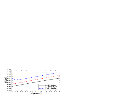
Figure 1: The values of the $df=\frac{d}{d\frac{1}{T^{2}}}\log\left[\frac{\alpha_{s}(T)}{\alpha_{s}(\mu)}\right]^{\frac{4}{9}}$ with variations of the Borel parameters.

3 Numerical Results

In calculations, we have assumed that the linear density approximation is valid at the low nuclear density. The input parameters are taken as $\langle q^{\dagger}q\rangle_{\rho_{N}}={3\over 2}\rho_{N}$, $\langle s^{\dagger}s\rangle_{\rho_{N}}=0$, $\langle\bar{q}q\rangle_{\rho_{N}}=\langle\bar{q}q\rangle+{\sigma_{N}\over m_{u}+m_{d}}\rho_{N}$, $\langle\bar{s}s\rangle_{\rho_{N}}=\langle\bar{s}s\rangle+y{\sigma_{N}\over m_{u}+m_{d}}\rho_{N}$, $\langle\frac{\alpha_{s}GG}{\pi}\rangle_{\rho_{N}}=\langle\frac{\alpha_{s}GG}{\pi}\rangle-(0.65\pm 0.15)\,{\rm GeV}\rho_{N}$, $\langle q^{\dagger}iD_{0}q\rangle_{\rho_{N}}=0.18\,{\rm GeV}\rho_{N}$, $\langle s^{\dagger}iD_{0}s\rangle_{\rho_{N}}=\frac{m_{s}}{4}\langle\bar{s}s\rangle_{\rho_{N}}+0.02\,{\rm GeV}\rho_{N}$, $m_{u}+m_{d}=12\,\rm{MeV}$, $\sigma_{N}=(45\pm 10)\,\rm{MeV}$, $\langle q^{\dagger}iD_{0}iD_{0}q\rangle_{\rho_{N}}+{1\over 12}\langle q^{\dagger}g_{s}\sigma Gq\rangle_{\rho_{N}}=0.031\,{\rm{GeV}}^{2}\rho_{N}$, $\langle s^{\dagger}iD_{0}iD_{0}s\rangle_{\rho_{N}}+{1\over 12}\langle s^{\dagger}g_{s}\sigma Gs\rangle_{\rho_{N}}=y0.031\,{\rm{GeV}}^{2}\rho_{N}$, $\langle\bar{q}g_{s}\sigma Gq\rangle=m_{0}^{2}\langle\bar{q}q\rangle$, $\langle\bar{s}g_{s}\sigma Gs\rangle=m_{0}^{2}\langle\bar{s}s\rangle$, $\langle\bar{q}iD_{0}iD_{0}q\rangle_{\rho_{N}}+{1\over 8}\langle\bar{q}g_{s}\sigma Gq\rangle_{\rho_{N}}=0.3\,{\rm{GeV}}^{2}\rho_{N}$, $\langle\bar{s}iD_{0}iD_{0}s\rangle_{\rho_{N}}+{1\over 8}\langle\bar{s}g_{s}\sigma Gs\rangle_{\rho_{N}}=y0.3\,{\rm{GeV}}^{2}\rho_{N}$, $\langle\bar{q}g_{s}\sigma Gq\rangle_{\rho_{N}}=\langle\bar{q}g_{s}\sigma Gq\rangle+3.0\,{\rm GeV}^{2}\rho_{N}$, $\langle\bar{s}g_{s}\sigma Gs\rangle_{\rho_{N}}=\langle\bar{s}g_{s}\sigma Gs\rangle+y3.0\,{\rm GeV}^{2}\rho_{N}$, $\langle q^{\dagger}g_{s}\sigma Gq\rangle_{\rho_{N}}=-0.33\,{\rm GeV}^{2}\rho_{N}$, $\langle s^{\dagger}g_{s}\sigma Gs\rangle_{\rho_{N}}=-y0.33\,{\rm GeV}^{2}\rho_{N}$, $\langle\bar{q}q\rangle=-(0.23\,\rm{GeV})^{3}$, $\langle\bar{s}s\rangle=0.8\langle\bar{q}q\rangle$, $m_{0}^{2}=0.8\,\rm{GeV}^{2}$, $\rho_{N}=(0.11\,\rm{GeV})^{3}$, $\langle\bar{q}q\rangle^{2}_{\rho_{N}}=f\langle\bar{q}q\rangle_{\rho_{N}}\times\langle\bar{q}q\rangle_{\rho_{N}}+(1-f)\langle\bar{q}q\rangle\times\langle\bar{q}q\rangle$, $\langle\bar{s}s\rangle^{2}_{\rho_{N}}=f\langle\bar{s}s\rangle_{\rho_{N}}\times\langle\bar{s}s\rangle_{\rho_{N}}+(1-f)\langle\bar{s}s\rangle\times\langle\bar{s}s\rangle$, $\langle\bar{q}q\rangle\langle\bar{s}s\rangle_{\rho_{N}}=f\langle\bar{q}q\rangle_{\rho_{N}}\times\langle\bar{s}s\rangle_{\rho_{N}}+(1-f)\langle\bar{q}q\rangle\times\langle\bar{s}s\rangle$, $\langle\frac{\alpha_{s}GG}{\pi}\rangle=(0.33\,\rm{GeV})^{4}$, $f=0.5\pm 0.5$, $y=0.3$, $m_{s}=0.13\,\rm{GeV}$ at the energy scale $\mu=1\,\rm{GeV}$ [9].

In the conventional QCD sum rules [7], there are two criteria (pole dominance and convergence of the operator product expansion) for choosing the Borel parameter $T^{2}$ and threshold parameter $s_{0}$. In this article, we take the pole contributions $R$ as $(45-80)\%$, just like the ones in our previous works on the heavy, doubly heavy and triply heavy baryon states [16], the pole contributions $R$ are defined by

$$R = \int_{0}^{s_{0}}dse^{-\frac{s}{T^{2}}}\rho(s)/\int_{0}^{\infty}dse^{-\frac{s}{T^{2}}}\rho(s)\,,$$ (11)

where the $\rho(s)$ denotes the QCD spectral densities, the integral over the $s$ can be carried out analytically, see Eqs.(9-10). In calculations, we observe that larger threshold parameters lead to larger Borel windows, and choose the possible smallest Borel windows, $T^{2}_{max}-T^{2}_{min}=0.4\,\rm{GeV}^{2}$, to obtain the lowest threshold parameters, and therefore obtain the possible lowest masses, which correspond to the largest correlation lengths, the revelent values are shown explicitly in Table 1. If the same threshold parameters are taken, the pole contributions are almost the same in the Borel windows for the QCD sum rules both in the vacuum and in the nuclear matter. Thereafter, we will not distinguish the pole contributions in the vacuum and in the nuclear matter. On the other hand, the main contributions come from the perturbative terms, the operator product expansion are well convergent, the two criteria of the QCD sum rules are satisfied.

Finally we obtain the numerical values of the masses and pole residues both in the vacuum and in the nuclear matter, which are also shown explicitly in Table 1 and Fig.2. The present predictions $\widehat{M}_{ud(0^{+})}=0.50\,\rm{GeV}$, $\widehat{M}_{ds(0^{+})}=0.64\,\rm{GeV}$ are larger than the values $\widehat{M}_{ud(0^{+})}=0.40\,\rm{GeV}$, $\widehat{M}_{ds(0^{+})}=0.46\,\rm{GeV}$ obtained in Ref.[14], where the derivative $\frac{1}{d\frac{1}{T^{2}}}$ does not act on the $\alpha_{s}(T)$. From Table 1 and Fig.2, we can see that including the renormalization group improvement factor $\left[\frac{\alpha_{s}(T)}{\alpha_{s}(\mu)}\right]^{\frac{4}{9}}$ reduces the diquark masses significantly, $M_{ud(0^{+})}-\widehat{M}_{ud(0^{+})}=0.14\,\rm{GeV}$, $M_{qs(0^{+})}-\widehat{M}_{qs(0^{+})}=0.13\,\rm{GeV}$, $M_{ud(1^{+})}-\widehat{M}_{ud(1^{+})}=0.11\,\rm{GeV}$, $M_{qs(1^{+})}-\widehat{M}_{qs(1^{+})}=0.12\,\rm{GeV}$. Although the factor $\left[\frac{\alpha_{s}(T)}{\alpha_{s}(\mu)}\right]^{\frac{4}{9}}\approx 1$, the terms associate with the derivative $\frac{d}{d\frac{1}{T^{2}}}\left[\frac{\alpha_{s}(T)}{\alpha_{s}(\mu)}\right]^{\frac{4}{9}}$ play an important role in the derived QCD sum rules. The values of the derivative $\frac{d}{d\frac{1}{T^{2}}}\log\left[\frac{\alpha_{s}(T)}{\alpha_{s}(\mu)}\right]^{\frac{4}{9}}$ are rather large compared with the diquark masses, see Fig.1 and Table 1.

The values of the in-vacuum diquark masses from different theoretical approaches vary in a large range, for examples, $M_{ud(0^{+})}=(0.14-0.74)\,\rm{GeV}$ [17], $M_{ud(0^{+})}=0.74\,\rm{GeV}$, $M_{qs(0^{+})}=0.88\,\rm{GeV}$, $M_{ud(1^{+})}=0.95\,\rm{GeV}$, $M_{qs(1^{+})}=1.05\,\rm{GeV}$ [18], $M_{ud(0^{+})}=0.82\,\rm{GeV}$, $M_{qs(0^{+})}=1.10\,\rm{GeV}$, $M_{ud(1^{+})}=1.02\,\rm{GeV}$, $M_{qs(1^{+})}=1.30\,\rm{GeV}$ [19], $M_{ud(0^{+})}=0.76\,\rm{GeV}$, $M_{qs(0^{+})}=0.98\,\rm{GeV}$ [20] from the Bethe-Salpeter equation with different confining potentials; $M_{ud(0^{+})}=0.710\,\rm{GeV}$, $M_{qs(0^{+})}=0.948\,\rm{GeV}$, $M_{ud(1^{+})}=0.909\,\rm{GeV}$, $M_{qs(1^{+})}=1.069\,\rm{GeV}$ from a relativistic quark model based on a quasipotential approach in QCD [21]; $M_{ud(0^{+})}=(0.694\pm 0.022)\,\rm{GeV}$, $M_{ud(1^{+})}-M_{ud(0^{+})}=(0.104\pm 0.042)\,\rm{GeV}$ from the lattice QCD [22]; $M_{ud(0^{+})}=(0.42\pm 0.03)\,\rm{GeV}$, $M_{ud(1^{+})}=(0.94\pm 0.02)\,\rm{GeV}$ [23], $M_{ud(0^{+})}=0.5\,\rm{GeV}$ [24] from the random instanton liquid model; $M_{ud(0^{+})}=0.234\,\rm{GeV}$, $M_{ud(1^{+})}=0.824\,\rm{GeV}$ from the Nambu-Jona-Lasinio Model [25]; $M_{ud(0^{+})}=0.395\,\rm{GeV}$, $M_{qs(0^{+})}=0.590\,\rm{GeV}$ from the constituent diquark model [26]; etc. One should be careful when using them, naively, we expect that they should obey the approximated $SU_{f}(3)$ symmetry and the hypersplitting color-spin interaction maybe account for the $0^{+}$ and $1^{+}$ diquark mass breaking effects.

Lattice QCD calculations indicate that the strong attraction in the scalar diquark channels favors the formation of good diquarks, the weaker attraction in the axial-vector diquark channels maybe form bad diquarks, the energy gap between the light-flavor axial-vector and scalar diquarks is about $\frac{2}{3}$ of the $\Delta$-nucleon mass splitting, $0.2\,\rm{GeV}$ [27], which is also expected from the hypersplitting color-spin interaction $\vec{T}_{i}\cdot\vec{T}_{j}\vec{\sigma}_{i}\cdot\vec{\sigma}_{j}$ [1, 5]. The coupled rainbow Dyson-Schwinger equation and ladder Bethe-Salpeter equation also indicate such an energy hierarchy [19]. In the present work, the central values have the energy gaps $M_{ud(1^{+})}-M_{ud(0^{+})}=0.17\,\rm{GeV}$, $M_{qs(1^{+})}-M_{qs(0^{+})}=0.15\,\rm{GeV}$, $\widehat{M}_{ud(1^{+})}-\widehat{M}_{ud(0^{+})}=0.20\,\rm{GeV}$, $\widehat{M}_{qs(1^{+})}-\widehat{M}_{qs(0^{+})}=0.16\,\rm{GeV}$, which are consistent with predictions of the lattice QCD and Bethe-Salpeter equation. If we neglect the uncertainties, the $SU_{f}(3)$ breaking effects for the masses of the scalar and axial-vector diquark states are $M_{qs(0^{+})}-M_{ud(0^{+})}=0.13\,\rm{GeV}$, $M_{qs(1^{+})}-M_{ud(1^{+})}=0.11\,\rm{GeV}$, $\widehat{M}_{qs(0^{+})}-\widehat{M}_{ud(0^{+})}=0.14\,\rm{GeV}$, $\widehat{M}_{qs(1^{+})}-\widehat{M}_{ud(1^{+})}=0.10\,\rm{GeV}$, respectively, which are consistent with the naive expectation $m_{s}-m_{q}\approx 0.13\,\rm{GeV}$.

From Table 1, we can see that the diquark states in the nuclear matter have larger masses than the corresponding ones in the vacuum, the in-medium effects lead to the mass-shifts $\delta M_{ud(0^{+})}=0.04\,\rm{GeV}$, $\delta M_{qs(0^{+})}=0.02\,\rm{GeV}$, $\delta\widehat{M}_{ud(0^{+})}=0.04\,\rm{GeV}$, $\delta\widehat{M}_{qs(0^{+})}=0.01\,\rm{GeV}$, $\delta M_{ud(1^{+})}=0.06\,\rm{GeV}$, $\delta M_{qs(1^{+})}=0.03\,\rm{GeV}$, $\delta\widehat{M}_{ud(1^{+})}=0.04\,\rm{GeV}$, $\delta\widehat{M}_{qs(1^{+})}=0.03\,\rm{GeV}$. Although the diquark masses have uncertainties originate from the Borel parameters, the mass-shifts survive approximately as the uncertainties are canceled out with each other, see Fig.2, the quark-quark correlation lengths are reduced slightly in the nuclear matter. Compared with the $ud$ diquark states, the $qs$ diquark states have much smaller mass-shifts, which attributes to the condensates of the $s$-quark obtain much smaller modifications than the corresponding ones of the $u$ and $d$-quarks. On the other hand, we can see that the pole residues in the vacuum and in the nuclear matter approximately have the same values, as the dominating contributions come from the perturbative terms.

	$T^{2}/s_{0}\,(\rm{GeV}^{2})$	pole	$M(\rm{GeV})$	$f(\rm{GeV}^{2})$
$ud(0^{+})$	$0.5-0.9/1.2$	$(45-78)\%$	$0.64\pm 0.06\,[0.68\pm 0.06]$	$0.264\pm 0.017\,[0.264\pm 0.016]$
$qs(0^{+})$	$0.6-1.0/1.4$	$(47-74)\%$	$0.77\pm 0.04\,[0.79\pm 0.04]$	$0.313\pm 0.013\,[0.312\pm 0.012]$
$ud(1^{+})$	$0.6-1.0/1.6$	$(48-76)\%$	$0.81\pm 0.06\,[0.87\pm 0.05]$	$0.228\pm 0.016\,[0.233\pm 0.012]$
$qs(1^{+})$	$0.7-1.1/1.8$	$(49-74)\%$	$0.92\pm 0.04\,[0.95\pm 0.03]$	$0.269\pm 0.011\,[0.269\pm 0.010]$
$\widehat{ud(0^{+})}$	$0.5-0.9/1.2$	$(45-77)\%$	$0.50\pm 0.05\,[0.54\pm 0.04]$	$0.246\pm 0.010\,[0.243\pm 0.009]$
$\widehat{qs(0^{+})}$	$0.6-1.0/1.4$	$(47-74)\%$	$0.64\pm 0.03\,[0.65\pm 0.03]$	$0.286\pm 0.007\,[0.283\pm 0.007]$
$\widehat{ud(1^{+})}$	$0.6-1.0/1.6$	$(48-77)\%$	$0.70\pm 0.04\,[0.74\pm 0.04]$	$0.209\pm 0.010\,[0.210\pm 0.008]$
$\widehat{qs(1^{+})}$	$0.7-1.1/1.8$	$(49-75)\%$	$0.80\pm 0.03\,[0.83\pm 0.02]$	$0.244\pm 0.006\,[0.242\pm 0.006]$

Table 1: The Borel parameters, threshold parameters, pole contributions, masses and pole residues of the light-flavor diquark states, the wide-hat  $\widehat{}$  denotes the renormalization group improvement factor $\left[\frac{\alpha_{s}(T)}{\alpha_{s}(\mu)}\right]^{\frac{4}{9}}$ is included, and the bracket denotes the values in the nuclear matter.

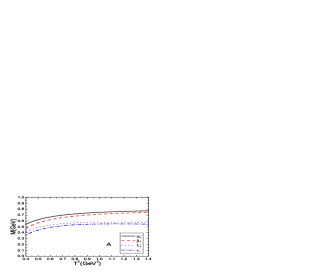
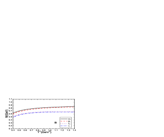
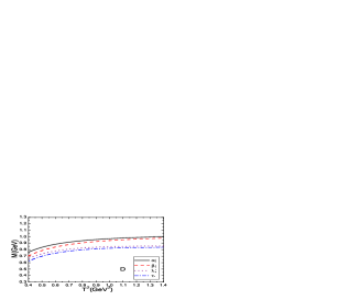
Figure 2: The masses $M$ of the light-flavor diquark states with variations of the Borel parameters $T^{2}$, the $A$, $B$, $C$ and $D$ correspond to the $ud(0^{+})$, $qs(0^{+})$, $ud(1^{+})$ and $qs(1^{+})$ diquark states respectively. The $\alpha$, $\lambda$ and $\beta$, $\tau$ denote the values from the QCD sum rules in the nuclear matter and in the vacuum respectively; while the $\lambda$, $\tau$ and $\alpha$, $\beta$ denote the renormalization group improvement factor $\left[\frac{\alpha_{s}(T)}{\alpha_{s}(\mu)}\right]^{\frac{4}{9}}$ is included and not included respectively.

4 Conclusion

In this article, we study the light-flavor scalar and axial-vector diquark states in the vacuum and in the nuclear matter using the QCD sum rules in an systematic way. The predicted diquark masses in the vacuum obey the flavor $SU_{f}(3)$ symmetry approximately, and the $0^{+}$ and $1^{+}$ diquark mass breaking effects are consistent with the lattice calculations. The diquark states in the nuclear matter have larger masses than the corresponding ones in the vacuum, the quark-quark correlation lengths are reduced slightly in the nuclear matter. We can take the diquark masses as basic parameters and perform many phenomenological analysis.

References

[1] A. De Rujula, H. Georgi and S. L. Glashow, Phys. Rev. D12 (1975) 147;
R. L. Jaffe, hep-ph/0001123.
[2] R. L. Jaffe, Phys. Rev. D15 (1977) 267; Phys. Rev. D15 (1977) 281.
[3] A. Selem and F. Wilczek, hep-ph/0602128; T. Friedmann, arXiv:0910.2229.
[4] M. Anselmino, E. Predazzi, S. Ekelin, S. Fredriksson
and D. B. Lichtenberg, Rev. Mod. Phys. 65 (1993) 1199.
[5] R. L. Jaffe, Phys. Rept. 409 (2005) 1.
[6] M. Oettel, G. Hellstern, R. Alkofer, H. Reinhardt, Phys. Rev. C58 (1998) 2459;
M. Oettel, R. Alkofer, L. von Smekal, Eur. Phys. J. A8 (2000) 553.
[7] M. A. Shifman, A. I. Vainshtein and V. I. Zakharov,
Nucl. Phys. B147 (1979) 385, 448; L. J. Reinders, H. Rubinstein and S. Yazaki, Phys. Rept. 127 (1985) 1.
[9] T. D. Cohen, R. J. Furnstahl, D. K. Griegel and X. M. Jin, Prog. Part. Nucl. Phys. 35 (1995)
221; X. M. Jin, T. D. Cohen, R. J. Furnstahl and D. K. Griegel, Phys. Rev. C47 (1993) 2882;
X. M. Jin, M. Nielsen, T. D. Cohen, R. J. Furnstahl and D. K. Griegel, Phys. Rev. C49 (1994) 464.
[10] E. G. Drukarev and E. M. Levin, Prog. Part. Nucl. Phys. 27 (1991)
77; E. G. Drukarev, M. G. Ryskin and V. A. Sadovnikova, Prog. Part.
Nucl. Phys. 47 (2001) 73; E. G. Drukarev, Prog. Part. Nucl. Phys. 50 (2003) 659.
[11] B. Friman et al, ”The CBM Physics Book: Compressed Baryonic Matter in Laboratory
Experiments”, Springer Heidelberg.
[12] M. F. M. Lutz et al, arXiv:0903.3905.
[13] H. G. Dosch, M. Jamin and B. Stech, Z. Phys. C42 (1989)
167; M. Jamin and M. Neubert, Phys. Lett. B238 (1990) 387.
[14] A. Zhang, T. Huang and T. G. Steele, Phys. Rev. D76 (2007) 036004.
[15] Z. G. Wang, Eur. Phys. J. C71 (2011) 1524.
[16] Z. G. Wang, Phys. Lett. B685 (2010) 59;
Z. G. Wang, Eur. Phys. J. C68 (2010) 479;
Z. G. Wang, Eur. Phys. J. C68 (2010) 459;
Z. G. Wang, Eur. Phys. J. A45 (2010) 267;
Z. G. Wang, Eur. Phys. J. A47 (2011) 81;
Z. G. Wang, arXiv:1112.2274.
[17] R. T. Cahill, C. D. Roberts, J. Praschifka, Phys. Rev. D36 (1987) 2804.
[18] C. J. Burden, L. Qian, C. D. Roberts, P. C. Tandy, M. J. Thomson, Phys. Rev. C55 (1997) 2649.
[19] P. Maris, Few Body Syst. 32 (2002) 41.
[20] Z. G. Wang, S. L. Wan, W. M. Yang, Commun. Theor. Phys. 47 (2007) 287.
[21] D. Ebert, R. N. Faustov, V. O. Galkin, Phys. Rev.D72 (2005) 034026.
[22] M. Hess, F. Karsch, E. Laermann, I. Wetzorke, Phys. Rev. D58 (1998) 111502.
[23] T. Schaefer, E. V. Shuryak, J. Verbaarschot, Nucl. Phys. B412 (1994) 143.
[24] M. Cristoforetti, P. Faccioli, G. Ripka, M. Traini, Phys. Rev. D71 (2005) 114010.
[25] U. Vogl, Z. Phys. A337 (1990) 191.
[26] L. Maiani, A. D. Polosa, F. Piccinini, V. Riquer, Phys. Rev. Lett. 93 (2004) 212002;
L. Maiani, F. Piccinini, A. D. Polosa, V. Riquer, Phys. Rev. D71 (2005) 014028.
[27] C. Alexandrou, P. de Forcrand and B. Lucini, Phys. Rev. Lett. 97 (2006) 222002.