Conversion of terahertz wave polarization at the boundary of a layered superconductor due to the resonance excitation of oblique surface waves

Abstract

We predict a complete TM$\leftrightarrow$TE transformation of the polarization of terahertz electromagnetic waves reflected from a strongly anisotropic boundary of a layered superconductor. We consider the case when the wave is incident on the superconductor from a dielectric prism separated from the sample by a thin vacuum gap. The physical origin of the predicted phenomenon is similar to the Wood anomalies known in optics, and is related to the resonance excitation of the oblique surface waves. We also discuss the dispersion relation for these waves, propagating along the boundary of the superconductor at some angle with respect to the anisotropy axis, as well as their excitation by the attenuated-total-reflection method.

Surface waves play a very important role in many fundamental resonant phenomena in different fields of modern physics. A well-known example of such phenomena are the Wood anomalies in the reflectivity and transmissivity of periodically-corrugated metal and semiconducting samples (see, e.g., Refs. agr, ; rae, ; pet, ; bar, ). A more recent example is the extraordinary transmission of light through metal films perforated by subwavelength holes ebb ; Marad . The excitation of surface plasmons can also result in an “inverse” effect of resonant suppression of light transmission through perforated metal films with thicknesses less than the skin-depth katz .

Recent interest on the effects listed above is also partly due to their possible applications, e.g., in photovoltaics, as well as the detection and filtering of radiation in the far-infrared and visible frequency ranges. From this point of view, it is interesting to consider layered superconductors, instead of metals, for designing devices which operate using the excitation of surface waves. Indeed, the characteristic frequencies of surface waves in these materials belong to the terahertz frequency range, which is important for different applications, but is still hard to reach for electronic and optical devices.

Layered superconductors are either artificially-grown stacks of Josephson junctions, e.g., Nb/Al-AlO_x/Nb, or natural high-temperature superconductors, such as $\rm Bi_{2}Sr_{2}CaCu_{2}O_{8+\delta}$. These materials contain thin superconducting layers separated by thicker dielectrics. Experiments on the $\mathbf{c}$-axis transport in layered superconductors justify the use of a theoretical model in which the superconducting layers are coupled by the intrinsic Josephson effect through the layers (see, e.g., Refs. Kl-Mu, ; Kl-Mu2, ). Due to their layered structure, these superconductors possess a strongly-anisotropic current capability.

The multi-layered structure of $\rm Bi_{2}Sr_{2}CaCu_{2}O_{8+\delta}$ (and similar superconductors) supports the propagation of specific Josephson plasma electromagnetic waves (JPWs) (see, e.g., the review  Thz-rev and references therein). The spectrum of JPWs lies above the so-called Josephson plasma frequency, $\omega_{J}\sim 1$ THz. In a semi-infinite sample, apart from bulk JPWs, surface Josephson plasma waves (SJPWs) can propagate along the interface between an external dielectric and a layered superconductor. These waves are similar to the surface plasmon-polaritons in normal metals. As shown in Refs. surf, , the spectrum of SJPWs also lies in the terahertz range and consists of two branches: one above $\omega_{J}$ and another below it. Similarly to the optical resonance phenomena in normal metals, the resonance excitation of SJPWs is accompanied by Wood anomalies in the reflection and transmission of terahertz waves through layered superconductors. However, the strong anisotropy of the current capability can result in new resonance phenomena, specific to layered superconductors.

In this paper, we predict one of such unusual resonance phenomena. We show that the resonance excitation of surface waves can be accompanied by a complete conversion of the polarization of the terahertz radiation after reflection from an anisotropic boundary of a layered superconductor. For example, if the incident wave has a transverse magnetic (TM) polarization (a wave with the magnetic field parallel to the sample surface), the reflected wave is completely transverse electric (TE) (with the electric field parallel to the sample surface), at an appropriate choice of the direction of the incident wave vector. We emphasize that this phenomenon is not an analog of the Brewster effect (where light with TM polarization, for a definite incidence angle, is perfectly transmitted through a transparent dielectric surface, with no reflection, and, therefore, the reflected light only contains the TE polarization). However, in the phenomenon predicted here, the reflected wave has a TE polarization when the incident radiation does not contain the wave with this polarization, i.e., when the incident wave is completely TM polarized. In other words, the reflected wave is TE-polarized due to the conversion of the incident TM radiation, but not due to separation of the TE wave from the incident mixed (TE+TM) radiation.

This polarization conversion has a clear physical explanation. We study here the so-called “attenuated-total-reflection” (ATR) method for producing surface waves. The surface wave is excited by the polarized radiation (with, e.g., TM polarization) incident on the superconductor from a dielectric semi-spherical prism separated from the sample by a thin vacuum gap (see Fig. 1).

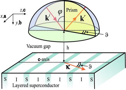
Figure 1: (Color online) Schematic geometry of the problem for the excitation of oblique surface waves. Here ${\bf k}^{i}$, ${\bf k}^{r}$, and $\bm{\kappa}$ are the wave vectors of the incident, reflected, and oblique surface waves. Note that S=superconductor and I=insulator.

We assume that the crystallographic c-axis of the superconductor lies in the sample surface, and, therefore, the boundary of the superconductor is strongly anisotropic. For arbitrary direction of the incident radiation, the wave vector $\bm{\kappa}$ of the excited surface wave is oriented at some angle $\vartheta$ with respect to the anisotropy axis c, and we call these waves oblique surface waves (OSWs) av . Due to the anisotropy, the OSWs contain all components of the electric and magnetic fields and, therefore, the radiation reflected from the superconductor contains waves of both, TM and TE, polarizations. In other words, due to the anisotropy, the reflected wave is, generally, unpolarized. Note that the ratio between the amplitudes of the reflected TM and TE waves is controlled by the parameters of the problem, such as the wave frequency $\omega$, angles $\vartheta$ and $\varphi$, the thickness $h$ of the vacuum gap, etc. The most important issue is the possibility to choose the angles $\vartheta$ and $\varphi$ for the incident radiation in such a way that the amplitude of the TM reflected wave vanishes. Recall that, in the isotropic case, one can choose the optimal value of the gap thickness $h$ to provide the complete suppression of the reflected wave under resonance conditions. Similarly, in the anisotropic case, we can choose the optimal value of the angle $\vartheta$ to provide the complete suppression of the reflected TM wave under resonance conditions. In this case, the desired complete conversion (TM $\rightarrow$ TE) of the polarization takes place.

Below we discuss the dispersion relation for oblique surface waves, obtain their excitations by the ATR method, and calculate the reflection coefficient $R_{\rm TM}$ for the TM wave and the conversion coefficient $T_{{\rm TM}\rightarrow{\rm TE}}$ for the mode conversion from TM to TE. Similar conversion phenomena can be observed for transitions from TE to TM modes, from incident ordinary waves to extraordinary ones, and from extraordinary waves to ordinary ones.

Oblique surface waves.— Consider a semi-infinite layered superconductor with the crystallographic c-axis parallel to the sample surface (see Fig. 2).

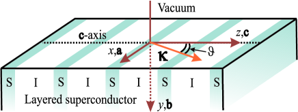
Figure 2: (Color online) Geometry for oblique surface waves.

We choose the coordinate system in such a way that the $z$-axis coincides with the crystallographic $\mathbf{c}$-axis of the superconductor and the $y$-axis is perpendicular to the sample surface. We study oblique surface waves, propagating along the interface vacuum-layered superconductor at an angle $\vartheta$ with respect to the c-axis, with electric $\mathbf{E}$ and magnetic $\mathbf{H}$ fields in the form,

$$\mathbf{E}(x,y,z,t),\>\mathbf{H}(x,y,z,t)\propto\exp[i(\bm{\kappa}\bm{\rho}-\omega t)],$$

where $\bm{\rho}=(x,z)$ is the radius vector in the $xz$-plane, $\bm{\kappa}=(k_{x},k_{z})$ is the wave vector of the oblique surface wave, $|\bm{\kappa}|>\omega/c$, and $c$ is the speed of light. It is suitable to present the electromagnetic field as a sum of two terms that correspond to the ordinary and extraordinary evanescent waves,

$$\mathbf{E}(y)=\mathbf{E}^{\rm(o)}(y)+\mathbf{E}^{\rm(e)}(y),\ \>\mathbf{H}(y)=\mathbf{H}^{\rm(o)}(y)+\mathbf{H}^{\rm(e)}(y).$$ (1)

The electric field of the ordinary wave and the magnetic field of the extraordinary wave are orthogonal to the anisotropy $z$-axis:

$$\mathbf{E}^{\rm(o)}_{z}(y)=\mathbf{H}^{\rm(e)}_{z}(y)=0.$$ (2)

For each of these waves, the Maxwell equations give the relations between the components of the electric $\mathbf{E}^{\rm vac}$ and magnetic $\mathbf{H}^{\rm vac}$ fields in the vacuum and the same exponential law for the decay of both waves along the $y$-axis,

$$\mathbf{E}_{\rm vac}^{\rm(o)}(y),\;\mathbf{E}_{\rm vac}^{\rm(e)}(y),\;\mathbf{H}_{\rm vac}^{\rm(o)}(y),\;\mathbf{H}_{\rm vac}^{\rm(e)}(y)\propto\exp(-ik_{y}^{\rm vac}y),$$ (3)

with imaginary normal component of the wave vector,

$$k_{y}^{\rm vac}=i(k_{x}^{2}+k_{z}^{2}-\omega^{2}/c^{2})^{1/2}.$$ (4)

The electromagnetic field inside the layered superconductor is determined by the distribution of the gauge-invariant phase difference $\chi$ of the order parameter between neighboring layers. This phase difference can be described by a set of coupled sine-Gordon equations (see review Thz-rev and references therein). In the continuum and linear approximation, $\chi$ can be excluded from the set of equations for electromagnetic fields, and the electrodynamics of layered superconductors can be described in terms of an anisotropic frequency-dependent dielectric permittivity with components $\varepsilon_{c}$ and $\varepsilon_{ab}$ across and along the layers, respectively negref ,

$$\begin{array}[]{l}\varepsilon_{c}(\Omega)=\varepsilon\left(1-\displaystyle\frac{1}{\Omega^{2}}+i\nu_{c}\displaystyle\frac{1}{\Omega}\right),\vspace{0.2cm}\\ \varepsilon_{ab}(\Omega)=\varepsilon\left(1-\displaystyle\frac{1}{\Omega^{2}}\gamma^{2}+i\nu_{ab}\displaystyle\frac{1}{\Omega}\gamma^{2}\right).\end{array}$$ (5)

Here we introduce the dimensionless parameters $\Omega=\omega/\omega_{J}$, $\nu_{ab}=4\pi\sigma_{ab}/\varepsilon\omega_{J}\gamma^{2}$, and $\nu_{c}=4\pi\sigma_{c}/\varepsilon\omega_{J}$, $\gamma=\lambda_{c}/\lambda_{ab}\gg 1$ is the current-anisotropy parameter, $\lambda_{c}=c/\omega_{J}\varepsilon^{1/2}$ and $\lambda_{ab}$ are the magnetic-field penetration depths along and across the layers, respectively. The relaxation frequencies $\nu_{ab}$ and $\nu_{c}$ are proportional to the averaged quasi-particle conductivities $\sigma_{ab}$ (along the layers) and $\sigma_{c}$ (across the layers), respectively; $\omega_{J}=(8\pi eDj_{c}/\hbar\varepsilon)^{1/2}$ is the Josephson plasma frequency. The latter is determined by the critical Josephson current density $j_{c}$, the interlayer dielectric constant $\varepsilon$, and the spatial period $D$ of the layered structure.

Contrary to the vacuum, the Maxwell equations give different laws for the decays of the ordinary and extraordinary waves in layered superconductors,

$$\mathbf{E}_{\rm s}^{\rm(o)}(y),\;\mathbf{H}_{\rm s}^{\rm(o)}(y)\propto\exp(ik_{{\rm s}y}^{\rm(o)}y)\>,$$

$$\mathbf{E}_{\rm s}^{\rm(e)}(y),\;\mathbf{H}_{\rm s}^{\rm(e)}(y)\propto\exp(ik_{{\rm s}y}^{\rm(e)}y)$$ (6)

with

$$k_{{\rm s}y}^{\rm(o)}=i(k_{x}^{2}+k_{z}^{2}-\omega^{2}\varepsilon_{ab}/c^{2})^{1/2}\>,$$ (7)

$$k_{{\rm s}y}^{\rm(e)}=i(k_{x}^{2}+k_{z}^{2}\varepsilon_{c}/\varepsilon_{ab}-\omega^{2}\varepsilon_{c}/c^{2})^{1/2}\>.$$ (8)

From the continuity conditions for the tangential components of the electric and magnetic fields at the interface $y=0$, we derive the dispersion equation of the OSWs,

$$k_{x}^{2}k_{z}^{2}(\varepsilon_{ab}-1)\displaystyle\frac{k_{{\rm s}y}^{\rm(o)}+k_{y}^{\rm vac}}{k_{{\rm s}y}^{\rm(o)}k_{y}^{\rm vac}}$$

$$-\Bigl{[}k_{z}^{2}(\varepsilon_{ab}-1)+\varepsilon_{ab}k_{y}^{\rm vac}(k_{y}^{\rm vac}+k_{{\rm s}y}^{\rm(e)})\Bigr{]}$$

$$\times\Bigl{[}\displaystyle\frac{1}{k_{{\rm s}y}^{\rm(o)}}\Bigl{(}\frac{\omega^{2}}{c^{2}}\varepsilon_{ab}-k_{z}^{2}\Bigr{)}+\displaystyle\frac{1}{k_{y}^{\rm vac}}\Bigl{(}\frac{\omega^{2}}{c^{2}}-k_{z}^{2}\Bigr{)}\Bigr{]}=0.$$ (9)

Figure 3 illustrates the numerically calculated dispersion curves of the OSWs for different values of the angle $\vartheta$.

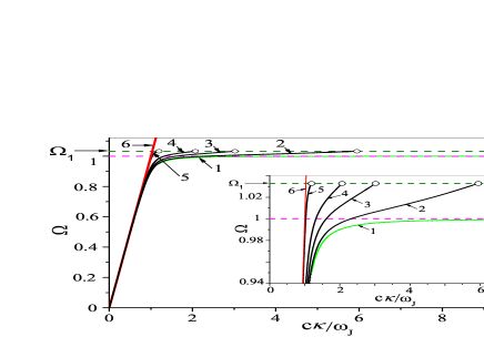
Figure 3: (Color online) Dispersion curves $\Omega(c\kappa/\omega_{J})$ of the OSWs for $\varepsilon=16$, $\gamma=200$, and $\nu_{ab}=\nu_{c}=0$. Curves 1–6 correspond to $\vartheta=0^{\circ}$, $10^{\circ}$, $20^{\circ}$, $30^{\circ}$, $60^{\circ}$, and $90^{\circ}$, respectively. The hollow circles at $\Omega=\Omega_{1}=\sqrt{\varepsilon/(\varepsilon-1)}$ show the end-points of the dispersion curves. In these points, the extraordinary wave, which is part of the OSW, is transformed into a bulk wave.

Excitation of the OSWs and the polarization conversion.— Here we investigate the OSWs excitation using the ATR method. Consider a TM polarized wave incident from a dielectric prism with permittivity $\varepsilon_{p}$ onto a layered superconductor separated from the prism by a vacuum gap of thickness $h$ (see Fig. 1). The incident angle $\varphi$ exceeds the limit angle $\theta_{t}=\arcsin(\varepsilon_{p}^{-1/2})$ for the total internal reflection. In this case the incident wave can excite a surface wave if the resonance condition, $\omega\varepsilon_{p}^{1/2}\sin\varphi=c\kappa$ is satisfied.

The electromagnetic field in the dielectric prism is a sum of three terms that correspond to the incident TM polarized wave and two reflected waves with the TM and TE polarizations. Thus, the $x$-component of the electric field in the prism can be presented as

$$E_{x}^{p}(x,y,z,t)=\left[E^{i}_{x}\exp(ik_{p\,y}y)\right.$$

$$\left.+(E^{r}_{x\>{\rm TM}}+E^{r}_{x\>{\rm TE}})\exp(-ik_{p\,y}y)\right]\exp\bigl{[}i(\bm{\kappa}\bm{\rho}-\omega t)\bigr{]}$$ (10)

where $E^{i}_{x}$, $E^{r}_{x\>{\rm TM}}$, and $E^{r}_{x\>{\rm TE}}$ are the amplitudes of the $x$-components of the electric field for the incident waves and for the reflected TM and TE waves, respectively; $k_{p\,y}=(\omega/c)\,\varepsilon_{p}^{1/2}\cos\varphi$ is the normal component of the wave vector of the incident and reflected waves. Other components of the electromagnetic field in the prism are expressed via the amplitudes $E^{i}_{x}$, $E^{r}_{x\>{\rm TM}}$, and $E^{r}_{x\>{\rm TE}}$ using the Maxwell equations.

In the vacuum gap, we define the electromagnetic field as the superposition of four evanescent waves. They are two TM modes with imaginary $y$-components $\pm k_{y}^{\rm vac}$ of the wave vectors given by Eq. (4) and two TE modes with the same wave vectors. In the layered superconductor we have, similarly to the previous section, ordinary and extraordinary waves with the normal components of the wave vectors given by Eqs. (7) and (8). Then, using the continuity boundary conditions for the tangential components of the electric and magnetic fields at the interfaces dielectric-vacuum and vacuum-layered superconductor, we obtain eight linear algebraic equations for eight unknown amplitudes (for 4 waves in the vacuum, 2 waves in the layered superconductor, and amplitudes $E^{r}_{x\>{\rm TM}}$, $E^{r}_{x\>{\rm TE}}$ of the reflected waves in the dielectric prism). Solving these equations, one can derive the reflectivity coefficient $R_{\rm TM}(\varphi,\vartheta)=|\textbf{E}^{r}_{\>{\rm TM}}|^{2}/|\textbf{E}^{i}|^{2}=|E^{r}_{x\>{\rm TM}}/E^{i}_{x}|^{2}$ for the TM wave and the coefficient $T_{{\rm TM}\rightarrow{\rm TE}}(\varphi,\vartheta)=|\textbf{E}^{r}_{\>{\rm TE}}|^{2}/|\textbf{E}^{i}|^{2}=|E^{r}_{x\>{\rm TE}}/E^{i}_{x}|^{2}\tan^{2}\vartheta\cos^{2}\varphi$ of the transformation from the TM mode to the TE one. Figure 4 shows the dependences of these coefficients on the angle $\varphi$, calculated for $\varepsilon_{p}=10$, $\varepsilon=16$, $\gamma=200$, $\Omega=1.00035$, $\nu_{ab}=\nu_{c}=10^{-3}$, $h=c/2\omega_{J}$, $\vartheta=15.6^{\circ}$.

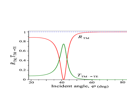
Figure 4: (Color online) The reflectivity $R_{\rm TM}$ and the transformation coefficient $T_{{\rm TM}\rightarrow{\rm TE}}$, both versus $\varphi$.

The curves demonstrate the complete transformation of the TM-polarized wave to the TE wave, for the optimal value of the angle $\vartheta=15.6^{\circ}$, under resonance condition. The positions of the minimum in the $R_{\rm TM}(\varphi)$ dependence and of the maximum in the $T_{{\rm TM}\rightarrow{\rm TE}}(\varphi)$ dependence coincide. This position corresponds to the most effective excitation of the oblique surface wave. Similar effects can be also observed for the TE$\rightarrow$TM complete transformation of the polarization, as well as for the complete transformation of the incident ordinary waves to extraordinary and vice versa. Figure 5 shows the dependences of the reflection coefficient $R_{\rm TE}(\varphi,\vartheta)$ and the coefficient $T_{{\rm TE}\rightarrow{\rm TM}}(\varphi,\vartheta)$ of the transformation from the TE mode to the TM one calculated for $\varepsilon_{p}=10$, $\varepsilon=16$, $\gamma=200$, $\Omega=1.0004$, $\nu_{ab}=\nu_{c}=10^{-3}$, $h=0.18c/\omega_{J}$, and $\vartheta=22^{\circ}$.

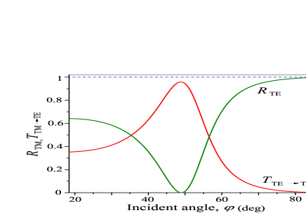
Figure 5: (Color online) The reflectivity $R_{\rm TE}$ and the transformation coefficient $T_{{\rm TE}\rightarrow{\rm TM}}$, both versus $\varphi$.

Conclusions.— We predict the complete polarization conversion for terahertz waves reflecting from the strongly-anisotropic surface of layered superconductors. The origin of this unusual effect is similar to the Wood anomalies known in optics, and is related to the resonance excitation of the oblique surface waves.

We acknowledge partial support from the NSA, LPS, ARO, NSF grant No. 0726909, JSPSRFBR Contract No. 09-02-92114, Kakenhi (S), MEXT, the JSPS-FIRST program, Ukrainian State Program on Nanotechnology, and the Program FPNNN of NAS of Ukraine (grant No 9/11-H).

References

- (1) V. M. Agranovich and D. L. Mills, Surface Polaritons (Nauka, Moscow, 1985).
- (2) H. Raether, Surface Plasmons (Springer, New York, 1988).
- (3) R. Petit, Electromagnetic Theory of Gratings (Springer, Berlin, 1980).
- (4) W. L. Barnes, A. Dereux, and T. W. Ebbesen, Nature 424, 824 (2003).
- (5) T. W. Ebbesenet al., Nature 391, 667 (1998).
- (6) A. V. Zayats, I. I. Smolyaninov, and A. A. Maradudin, Phys. Rep. 408, 131 (2005).
- (7) I. S. Spevak et al., Phys. Rev. B79, 161406 (2009).
- (8) R. Kleiner et al., Phys. Rev. Lett. 68, 2394 (1992).
- (9) R. Kleiner and P. Muller, Phys. Rev. B49, 1327 (1994).
- (10) S. Savel’ev et al., Rep. Prog. Phys. 73, 026501 (2010).
- (11) S. Savel’ev et al., Phys. Rev. Lett. 95, 187002 (2005); V. A. Yampol’skii et al., Phys. Rev. B76, 224504 (2007); A. V. Kats et al., Phys. Rev. B79, 214501 (2009); V. A. Golick et al., Phys. Rev. Lett. 104, 187003 (2010).
- (12) Yu. O. Averkov and V. M. Yakovenko, Phys. Rev. B81, 045427 (2010); J. Opt. Soc. Am. B 28, 155 (2011).
- (13) A. L. Rakhmanov et al., Phys. Rev. B 81, 075101 (2010).