On supersymmetric interfaces for string theory

Yuji  Satoh

Institute of Physics, University of Tsukuba

Tsukuba, Ibaraki 305-8571, Japan

Abstract

We construct the world-sheet interface which preserves space-time supersymmetry in type II superstring theories in the Green-Schwarz formalism. This is an analog of the conformal interface in two-dimensional conformal field theory. We show that a class of the supersymmetric interfaces generates T-dualities of type II theories, and that these interfaces have a geometrical interpretation in the doubled target space. We compute the partition function with a pair of the supersymmetric interfaces inserted, from which we read off the spectrum of the modes coupled to the interfaces and the Casimir energy between them. We also derive the transformation rules under which a set of D-branes is transformed to another by the interface.

December 2011

1 Introduction

Since its discovery, the D-brane has been a central subject in the study of superstring theory. On one hand, it preserves space-time supersymmetry and, on the other, it preserves world-sheet conformal invariance. As is generally the case for those which preserve fundamental symmetries, the D-brane plays an important and fundamental role in the theory. From the world-sheet point of view, a natural generalization of the D-brane or the conformal boundary/boundary state is the conformal interface [1, 2, 3]. It is a one-dimensional domain wall/defect in the world-sheet which preserves the conformal invariance and glues two generally different conformal field theories (CFTs). As anticipated, the conformal interface has interesting properties: it generates symmetries of CFT including T-dualities [4], and transforms a set of D-branes to another [5, 6]. For the aspects of the conformal interface, we refer to [7, 8, 9, 10, 11, 12, 13, 14, 15, 16, 17, 18] and references therein.

One can thus expect that, once embedded in superstring theory, the interface would provide an important element in order to explore non-perturbative aspects and symmetries of superstring theory. The purpose of this paper is to take a step toward this direction. In particular, we will study the world-sheet interface in type II superstring theories in flat space-time in the Green-Schwarz (GS) formalism. The reason to work in the GS formalism is two-fold. First, space-time supersymmetry is manifest and one can avoid complications due to ghosts, as usual. Second, a difficulty has been pointed out [3] for the conformal interface in the world-sheet of strings: the interface generally may not preserve enough Virasoro symmetries to remove negative norm states, except in the special cases where two sets of the Virasoro symmetries are preserved. In the GS formalism, the physical space is manifestly unitary, and hence this formalism should provide a safe framework in which one can study the object whose properties are yet to be investigated. As the genus of the world-sheet increases, the interface can be wrapped on non-equivalent one-cycles. In order for the interface to make full sense in string theory, it is necessary to clarify how to perform the summation over the genus for correlation functions involving interfaces. This is an important issue for future, and we focus on fixed genus in this paper.

In the GS formulation, the conformal boundary state describing the D-brane in the covariant formulation is represented as the boundary state preserving space-time supersymmetry [19]. Similarly, the conformal interface would be represented in the GS formulation as the interface preserving the space-time supersymmetry. In this paper, we indeed construct the world-sheet interface with this property. Since the world-sheet theory in the GS formulation is not a conformal field theory due to the gauge fixing, we call the above boundary states/interfaces the supersymmetric boundary states/interfaces. We find two classes of the supersymmetric interfaces, which are regarded as generalizations of the $c=1$ permeable conformal interfaces [3]. One describes factorized D-branes/boundary states, whereas the other is an analog of the topological conformal interface [2]. We show that the latter class generates T-dualities of type II theories. In both cases, two sets of the Virasoro generators in the physical space are preserved, and the difficulty mentioned above may be evaded. We also study properties of the supersymmetric interface. First, in parallel with the topological conformal interface [10], we see that the corresponding supersymmetric interface has a geometrical interpretation in the doubled target space. Second, we compute the coupling of the massless fields through the interface, and confirm the Buscher rules at the linearized level in the case of the analog of the topological interface. Third, we compute the partition function with a pair of an interface and its conjugate inserted, from which we read off the spectrum of the modes coupled to the interfaces and the Casimir energy between them. Finally, we derive the transformations of the D-branes by the interface. Our results confirm that the conformal interface is embedded into superstring theory at least for fixed genus, though somewhat in disguise in our formulation.

The rest of this paper is organized as follows. In section 2, we summarize the supersymmetric boundary state for type II superstrings in the GS formalism, together with the unfolding procedure of boundary states to interfaces. In section 3, we construct the supersymmetric interfaces. In section 4, we study the target-space geometry and the coupling of the massless fields. In section 5, we compute the partition function with the interfaces inserted. In section 6, we derive the transformations of the D-branes. We conclude with a summary and discussion in section 7.

2 Supersymmetric boundary states

The conformal interface in two-dimensional conformal field theory is obtained from the conformal boundary state by the unfolding procedure [1, 3]. In type II superstring theories in the Green-Schwarz formalism in light-cone gauge, the conformal symmetry is fixed, and the guiding principle to construct the boundary state, the conformal invariance, is replaced by the invariance under the space-time supersymmetry. Accordingly, the conformal boundary state, corresponding to the D-brane, is realized as the supersymmetric boundary state preserving space-time supersymmetry. It is then expected that the supersymmetric interface in the GS formalism is obtained by unfolding the supersymmetric boundary state. This is the strategy which we take in the following. We thus start our discussion with a summary on the supersymmetric boundary state [19] and the unfolding procedure.

2.1 Supersymmetric boundary states in type IIB theory

To be concrete, we first concentrate on type IIB theory in flat space-time. In the GS formalism in light-cone gauge, one of the light-cone string coordinates is parametrized as $X^{+}=x^{+}+p^{+}\tau$. The physical degrees of freedom are given by eight transverse coordinates, $X^{I}(\tau,\sigma)$ $(I=1,...,8)$, and two right- and left-moving SO(8) Majorana-Weyl spinors with the same chirality, $S^{a}(\tau-\sigma)$ and $\tilde{S}^{a}(\tau+\sigma)$ $(a=1,...,8)$. The other light-cone coordinate $X^{-}$ is determined through the constraints,

$$p^{+}\partial_{\pm}X^{-}=\partial_{\pm}X_{I}\partial_{\pm}X^{I}+\frac{i}{2}S^{a}\partial_{-}S^{a}+\frac{i}{2}\tilde{S}^{a}\partial_{+}\tilde{S}^{a}\,.$$ (2.1)

The half of the space-time supersymmetry is realized linearly by the spinor zero modes,

$$Q^{a}:=\sqrt{2p^{+}}S_{0}^{a}\,,\quad\tilde{Q}^{a}:=\sqrt{2p^{+}}\tilde{S}_{0}^{a}\,,$$ (2.2)

whereas the other half is realized non-linearly by

$$Q^{\dot{a}}:=\frac{1}{\sqrt{p^{+}}}\sigma_{a\dot{a}}^{I}\sum_{n=-\infty}^{\infty}S_{-n}^{a}\alpha_{n}^{I}\,,\quad\tilde{Q}^{\dot{a}}:=\frac{1}{\sqrt{p^{+}}}\sigma_{a\dot{a}}^{I}\sum_{n=-\infty}^{\infty}\tilde{S}_{-n}^{a}\tilde{\alpha}_{n}^{I}\,.$$ (2.3)

The modes of the fields satisfy the relations,

$$[\alpha_{m}^{I},\alpha_{n}^{J}]=m\delta_{m+n,0}\delta^{IJ}\,,\quad\{S_{m}^{a},S_{n}^{b}\}=\delta_{m+n,0}\delta^{ab}\,,$$ (2.4)

and similar ones for $\tilde{\alpha}_{n}^{I},\tilde{S}_{n}^{a}$. The matrices $\sigma^{I}_{a\dot{a}}$ together with $\bar{\sigma}^{I}_{\dot{a}a}(=\sigma^{I}_{a\dot{a}})$ form eight-dimensional gamma matrices

$$\gamma^{I}=\biggl{(}\begin{array}[]{cc}0&\sigma^{I}\\ \bar{\sigma}^{I}&0\end{array}\biggr{)}\quad{\rm satisfying}\quad\{\gamma^{I},\gamma^{J}\}=2\delta^{IJ}\,.$$ (2.7)

The anti-commutation relations among the supercharges are, e.g.,

$$\{Q^{a},Q^{b}\}=2p^{+}\delta^{ab}\,,\quad\{Q^{a},Q^{\dot{a}}\}=\sqrt{2}\alpha_{0}^{I}\sigma^{I}_{a\dot{a}}\,,\quad\{Q^{\dot{a}},Q^{\dot{b}}\}=P^{-}\delta^{\dot{a}\dot{b}}\,,$$ (2.8)

where

$$P^{-}=\frac{2}{p^{+}}\Bigl{(}\frac{1}{2}\alpha_{0}^{I}\alpha_{0}^{I}+N_{\rm b}+N_{\rm f}\Bigr{)}\,,$$ (2.9)

and

$$N_{\rm b}=\sum_{n=1}^{\infty}\alpha_{-n}^{I}\alpha_{n}^{I}\,,\quad N_{\rm f}=\sum_{n=1}^{\infty}nS_{-n}^{a}S_{n}^{a}\,.$$ (2.10)

The supersymmetric boundary state $|{\cal B}\rangle$ is defined to preserve half the supercharges,

$$(Q^{a}+iM_{ab}\tilde{Q}^{b})|{\cal B}\rangle=(Q^{\dot{a}}+iM_{\dot{a}\dot{b}}\tilde{Q}^{\dot{b}})|{\cal B}\rangle=0\,.$$ (2.11)

One finds that these conditions are satisfied by

$$|{\cal B}\rangle = {C}_{{\cal B}}\prod_{n=1}^{\infty}\exp\biggl{[}\frac{1}{n}M_{IJ}\alpha_{-n}^{I}\tilde{\alpha}_{-n}^{J}-iM_{ab}S_{-n}^{a}\tilde{S}_{-n}^{b}\biggr{]}|{\cal B}\rangle_{0}\,.$$ (2.12)

Here, ${C}_{{\cal B}}$ is the normalization constant. The zero-mode part $|{\cal B}\rangle_{0}=|{\cal B}\rangle_{\rm b0}|{\cal B}\rangle_{\rm f0}$ is annihilated by all the positive modes and given by

$$|{\cal B}\rangle_{\rm b0} = \sum|k^{I},k^{K}M_{KJ}\rangle\,,$$

$$|{\cal B}\rangle_{\rm f0} = M_{IJ}|I\rangle_{R}|J\rangle_{L}-iM_{\dot{a}\dot{b}}|\dot{a}\rangle_{R}|\dot{b}\rangle_{L}\,.$$ (2.13)

The summation symbol stands for the summation/integral over possible zero modes with appropriate weight. The bosonic zero modes act on the oscillator vacuum as $\alpha_{0}^{K}|k^{I},\tilde{k}^{J}\rangle=(k^{K}/2)|k^{I},\tilde{k}^{J}\rangle$, $\tilde{\alpha}_{0}^{K}|k^{I},\tilde{k}^{J}\rangle=(\tilde{k}^{K}/2)|k^{I},\tilde{k}^{J}\rangle$, whereas the spinor zero modes as

$$S_{0}^{a}|\dot{a}\rangle_{R}=\frac{1}{\sqrt{2}}\bar{\sigma}^{I}_{\dot{a}a}|I\rangle_{R}\,,\quad S_{0}^{a}|I\rangle_{R}=\frac{1}{\sqrt{2}}\sigma^{I}_{a\dot{a}}|\dot{a}\rangle_{R}\,,$$ (2.14)

for the right movers and similarly for the left movers. The matrices $(M_{IJ},M_{ab},M_{\dot{a}\dot{b}})$ are taken to be orthogonal ones,

$$M_{KL}=\exp\Bigl{[}\Omega_{IJ}\Sigma^{IJ}\Bigr{]}_{KL}\,,\quad M_{\alpha\beta}=\exp\Bigl{[}\frac{1}{2}\Omega_{IJ}\gamma^{IJ}\Bigr{]}_{\alpha\beta}=\biggl{(}\begin{array}[]{cc}M_{ab}&0\\ 0&M_{\dot{a}\dot{b}}\end{array}\biggr{)}\,,$$ (2.17)

where $(\Sigma^{IJ})_{KL}=\delta^{I}_{K}\delta^{J}_{L}-\delta^{J}_{K}\delta^{I}_{L}$, $\gamma^{IJ}=(\gamma^{I}\gamma^{J}-\gamma^{J}\gamma^{I})/2$ and $\Omega_{IJ}=-\Omega_{JI}$ are parameters. These SO(8) matrices are related by

$$\gamma^{K}M_{KI}=M\gamma^{I}M^{T}\,,$$ (2.18)

which reads in terms of the $8\times 8$ matrices $\sigma_{a\dot{a}}^{K}M_{KI}=M_{ab}\sigma^{I}_{b\dot{b}}M_{\dot{a}\dot{b}}\,.$ On the boundary state, the modes of the fields satisfy the boundary conditions,

$$(\alpha_{n}^{I}-M_{IJ}\tilde{\alpha}_{-n}^{J})|{\cal B}\rangle=(S^{a}_{n}+iM_{ab}\tilde{S}_{-n}^{b})|{\cal B}\rangle=0\,.$$ (2.19)

These are translated into the conditions on the fields at $\tau=0$ by using the mode expansions $\partial_{-}X^{AI}=\sum\alpha_{n}^{AI}e^{-2in(\tau-\sigma)}$, $S^{Aa}=\sum S_{n}^{Aa}e^{-2in(\tau-\sigma)}$ and similar ones for the left movers. Successively acting on the boundary state with the combinations of the supercharges and modes in (2.11) and (2.19) yields consistency conditions. One can check that these are satisfied by the orthogonality of the matrices, the relation (2.18) and the constraint $P^{-}=\tilde{P}^{-}$ which follows from (2.1).

A simple example of the supersymmetric boundary state is given by setting $M_{IJ}$ and $M_{\alpha\beta}$ to be

$$M^{(p)}_{IJ}=\biggl{(}\begin{array}[]{cc}-{\bf 1}_{p+1}&0\\ 0&{\bf 1}_{7-p}\end{array}\biggr{)}\,,\qquad M^{(p)}_{\alpha\beta}=\gamma^{1}\cdot\cdot\cdot\gamma^{p+1}\,,$$ (2.22)

where ${\bf 1}_{n}$ is the $n\times n$ unit matrix. This corresponds to the Neumann conditions (in the open string channel) for $I=1,...,p+1$ and the Dirichlet conditions for $I=p+2,...,8$. Furthermore, in light-cone gauge, it follows that $\partial_{\sigma}X^{\pm}=0$ from the gauge fixing condition and the constraints (2.1) . This means that one also has the Dirichlet conditions in the light-cone directions. The boundary state thus represents the $(p+1)$-instanton, which is related to the usual D$p$-brane by a double Wick rotation. Keeping this relation in mind, we use the terminology “D-brane” also for the boundary state in this paper. One can check that the coupling of the massless closed string modes to the boundary state agrees with that to the (Wick rotated) black $p$-brane. General supersymmetric boundary states are obtained by SO(8) transformations of $M^{(p)}_{IJ}$ and $M^{(p)}_{\alpha\beta}$. In particular, the sign of $M_{\alpha\beta}$ is flipped by a $2\pi$-rotation in all directions, which transforms a BPS state to an anti-BPS state. Note also that the forms of the matrices in (2.22) are compatible with (2.17) only when $p$ is odd.

2.2 Supersymmetric boundary states in type IIA theory

One can similarly construct the supersymmetric boundary state in type IIA theory by flipping the chirality for the left movers, e.g., $\tilde{S}^{a}\to\tilde{S}^{\dot{a}}$ and $|\dot{a}\rangle_{L}\to|a\rangle_{L}$. In this case, the boundary conditions for the supercharges become

$$(Q^{a}+iM_{a\dot{b}}\tilde{Q}^{\dot{b}})|{\cal B}\rangle=(Q^{\dot{a}}+iM_{\dot{a}b}\tilde{Q}^{b})|{\cal B}\rangle=0\,,$$ (2.23)

where $\tilde{Q}^{\dot{a}}=\sqrt{2p^{+}}\tilde{S}^{\dot{a}}$ are the supercharges for the linearly realized supersymmetry and $\tilde{Q}^{a}$, which are defined similarly to (2.3), are those for the non-linearly realized supersymmetry. The SO(8) matrices in (2.17) are multiplied by matrices generating reflections. The resultant matrices satisfy the relation (2.18) as before. For instance, for the usual D$p$-brane with even $p$, one has $M^{(p)}_{IJ}$ in (2.22) with even $p$ and

$$M^{(p)}_{\alpha\beta}=\gamma^{9}\gamma^{1}\cdot\cdot\cdot\gamma^{p+1}=\biggl{(}\begin{array}[]{cc}0&M_{a\dot{b}}\\ M_{\dot{a}b}&0\end{array}\biggr{)}\,.$$ (2.26)

The boundary state in type IIA theory then takes the form which is obtained from (2.12) and (2.1) by replacing $\tilde{S}_{n}^{a},(M_{ab},M_{\dot{a}\dot{b}})$ and $|\dot{b}\rangle_{L}$ with $\tilde{S}_{n}^{\dot{a}},(M_{a\dot{b}},M_{\dot{a}b})$ and $|b\rangle_{L}$, respectively.

2.3 Unfolding procedure

In two-dimensional CFT, a way to construct conformal interfaces is to unfold conformal boundary states. Suppose that one has a boundary state $|{\cal B}\rangle_{\rm CFT}=\sum_{i,j}c_{ij}|{\cal B}_{i}\rangle_{1}\otimes|{\cal B}_{j}\rangle_{2}$ in a tensor product theory CFT${}_{1}\otimes$CFT₂, which satisfies

$$0=(L^{1}_{n}+L^{2}_{n}-\tilde{L}^{1}_{-n}-\tilde{L}^{2}_{-n})|{\cal B}\rangle_{\rm CFT}\,.$$ (2.27)

Here, $c_{ij}$ are coefficients and $L_{n}^{A},\tilde{L}_{n}^{A}$ $(A=1,2)$ are the Virasoro generators for the right and left movers in CFT_A, respectively. Then, one can obtain a conformal interface gluing CFT₁ and CFT₂ by unfolding the boundary state as

$${\cal I}=\sum_{i,j}c_{ij}|{\cal B}_{i}\rangle_{1}\cdot{}_{2}\overline{\langle{\cal B}_{j}|}\,,$$ (2.28)

where ${}_{2}\overline{\langle{\cal B}_{j}|}$ is obtained from $|{\cal B}_{j}\rangle_{2}$ by the hermitian conjugation followed by the sign flip of the world-sheet coordinate $\tau\to-\tau$. (See Figure 1.) The resultant interface indeed preserves the conformal invariance,

$$(L^{1}_{n}-\tilde{L}^{1}_{-n}){\cal I}={\cal I}(L^{2}_{n}-\tilde{L}^{2}_{-n})\,,$$ (2.29)

which also means the conservation of energy across the world-sheet interface/defect ${\cal I}$. In this construction, the interface is located at $\tau=0$ in the world-sheet.

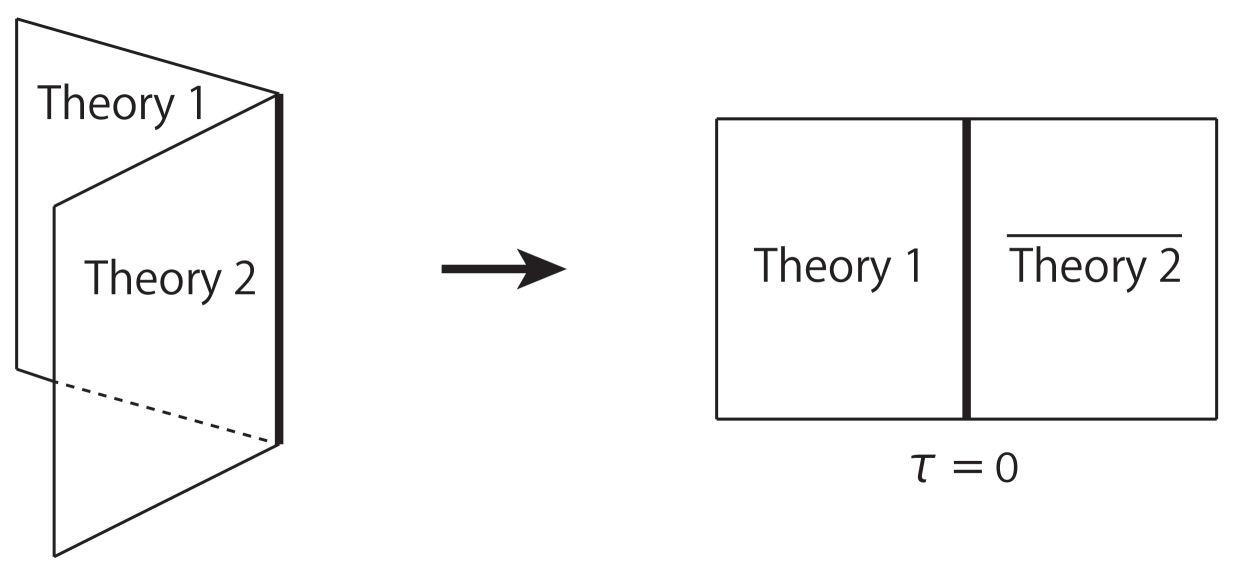
Figure 1: Unfolding procedure. A boundary state in a tensor product theory is unfolded to an interface gluing theory 1 and 2.

3 Supersymmetric interfaces

As we observed in the previous section, the supersymmetric boundary state represents the D-brane and is regarded as an analog of the conformal boundary state. In this section, we construct the supersymmetric interface by unfolding the supersymmetric boundary state, similarly to the conformal interface.

3.1 Case of type IIB theory

To be specific, in this subsection we consider the world-sheet interface which glues two type IIB theories residing on the left and the right side of the interface, respectively (IIB-IIB case). The interface is defined to satisfy the conditions on the supercharges,

$$(Q_{1}^{a}+iR^{1}_{ab}\tilde{Q}_{1}^{b}){\cal I} = {\cal I}(Q_{2}^{a}+iR^{2}_{ab}\tilde{Q}_{2}^{b})\,,$$ (3.1)

$$(Q_{1}^{\dot{a}}+iR^{1}_{\dot{a}\dot{b}}\tilde{Q}_{1}^{\dot{b}}){\cal I} = {\cal I}(Q_{2}^{\dot{a}}+iR^{2}_{\dot{a}\dot{b}}\tilde{Q}_{2}^{\dot{b}})\,,$$ (3.2)

for some $R^{A}_{ab},R^{A}_{\dot{a}\dot{b}}$ $(A=1,2)$. According to the unfolding procedure, we first double the fields, and denote the resultant modes by

$$(\alpha_{n}^{AI},\tilde{\alpha}_{n}^{AI})\,,\quad(S^{Aa}_{n},\tilde{S}^{Aa}_{n})\,.$$ (3.3)

We remark that we have doubled the fields just as an intermediate step for the construction. Then, one may consider a boundary state in which the bilinear forms of the oscillators are given by ${\cal S}_{AB}^{IJ}\alpha_{-n}^{AI}\tilde{\alpha}_{-n}^{BJ}$ and ${\cal S}_{AB}^{ab}S_{-n}^{Aa}\tilde{S}_{-n}^{Bb}$, where ${\cal S}_{AB}$’s are the “S-matrix” which determines the boundary conditions of the modes. Next, by unfolding the sector with $A=2$, one finds that the oscillators are transformed as $(\alpha_{n}^{2I},\tilde{\alpha}_{n}^{2I})\to(-\tilde{\alpha}_{-n}^{2I},-\alpha_{-n}^{2I})$ and $(S^{2a}_{n},\tilde{S}^{2a}_{n})\to(\tilde{S}^{2a}_{-n},S^{2a}_{-n})$. This results in an interface of the form

$${\cal I} = {C}_{{\cal I}}\,{\cal I}_{\rm b}\cdot{\cal I}_{\rm f}\,,$$

$${\cal I}_{\rm b}=\prod_{n=1}^{\infty}\exp\biggl{[}\frac{1}{n}\beta_{-n}^{AI}\cdot{\cal S}_{AB}^{IJ}\cdot\tilde{\beta}_{-n}^{BJ}\biggr{]}\cdot{\cal I}_{\rm b0}\,,$$

$${\cal I}_{\rm f}=\prod_{n=1}^{\infty}\exp\biggl{[}-iT_{-n}^{Aa}\ast{\cal S}_{AB}^{ab}\ast\tilde{T}_{-n}^{Bb}\biggr{]}\cdot{\cal I}_{\rm f0}\,.$$

Here, the oscillators are defined by

$$\beta_{n}^{AI}:=(\alpha_{n}^{1I},-\tilde{\alpha}_{-n}^{2I})\,,\quad\tilde{\beta}_{n}^{AI}:=(\tilde{\alpha}_{n}^{1I},-\alpha_{-n}^{2I})\,,$$

$$T_{n}^{Aa}:=(S_{n}^{1a},-\tilde{S}_{-n}^{2a})\,,\quad\tilde{T}_{n}^{Aa}:=(\tilde{S}_{n}^{1a},-S_{-n}^{2a})\,,$$ (3.5)

and the product $\ast$ by

$$U_{A}\ast V_{A}:=\eta_{AB}U_{A}V_{B}\,,$$ (3.6)

with $\eta_{AB}=\operatorname{diag}(+1,-1)$. (We do not raise or lower the indices $A,B$ by $\eta_{AB}$.) ${C}_{{\cal I}}$ is the normalization constant. It is also understood that the annihilation operators, or the oscillators with $A=2$, act on the interface implicitly from the right, e.g.,

$$\exp\Bigl{[}\alpha_{-n}^{1I}\alpha_{n}^{2J}\Bigr{]}\cdot{\cal I}=\sum_{l}\frac{1}{l!}(\alpha_{-n}^{1I})^{l}\cdot{\cal I}\cdot(\alpha_{n}^{2J})^{l}\,.$$ (3.7)

Starting from our ansatz of the form of the interface (3.1), we would like to determine $S_{AB}^{IJ}$, $S_{AB}^{ab}$ and the zero-mode factors ${\cal I}_{\rm b0},{\cal I}_{\rm f0}$, as well as $R^{A}_{ab}$, $R^{A}_{\dot{a}\dot{b}}$ in (3.1), (3.2).

For this purpose, we first note that the oscillators satisfy the continuity conditions on the interface, $\beta_{n}^{AI}\approx{\cal S}_{AB}^{IJ}\tilde{\beta}_{-n}^{BJ}$, $\tilde{\beta}_{n}^{AI}\approx\beta_{-n}^{BJ}{\cal S}_{BA}^{JI}$ and $T_{n}^{Aa}\approx-i{\cal S}_{AB}^{ab}\ast\tilde{T}_{-n}^{Bb}$, $\tilde{T}_{n}^{Aa}\approx+iT_{-n}^{Bb}\ast{\cal S}_{BA}^{ba}$ for $n\geq 1$. The symbol $\approx$ denotes the relations which hold on the interface. For example, $\beta_{n}^{1I}\approx{\cal S}_{1B}^{IJ}\tilde{\beta}_{-n}^{BJ}$ stands for $(\alpha_{n}^{1I}-{\cal S}_{11}^{IJ}\tilde{\alpha}_{-n}^{1J}){\cal I}={\cal I}(-{\cal S}_{12}^{IJ}\alpha^{2J}_{n})$. Next, we require that all the modes with $n\in{\mathbb{Z}}$ have the same transformations so that the continuity conditions give linear transformations of the fields. This leads to the condition that $S_{AB}^{IJ}$ is orthogonal and $S_{AB}^{ab}$ is pseudo-orthogonal,

$${\cal S}_{AB}^{IJ}{\cal S}_{AC}^{IK}=\delta^{JK}\delta_{BC}\,,\quad{\cal S}_{AB}^{ab}\ast{\cal S}_{AC}^{ac}=\delta^{bc}\eta_{BC}\,.$$ (3.8)

The continuity conditions on the oscillators are then summarized as

$$\beta_{n}^{AI}\approx{\cal S}_{AB}^{IJ}\tilde{\beta}_{-n}^{BJ}\,,\quad T_{n}^{Aa}\approx-i{\cal S}_{AB}^{ab}\ast\tilde{T}_{-n}^{Bb}\,,$$ (3.9)

for $n\neq 0$. Furthermore, in order for $(\alpha_{0}^{AI},\tilde{\alpha}_{0}^{AI})$ to have the same transformations as the non-zero modes, the bosonic zero-mode factor ${\cal I}_{\rm b0}$ should be of the form,

$${\cal I}_{\rm b0}=\sum|k^{1I},k^{BI^{\prime}}{\cal S}^{I^{\prime}J}_{B1}\rangle_{1}\cdot{}_{2}\langle-k^{2K},-k^{BI^{\prime}}{\cal S}^{I^{\prime}L}_{B2}|\,.$$ (3.10)

On the dual vacuum $(\alpha_{0}^{I},\tilde{\alpha}_{0}^{I})$ act as $\langle\tilde{k}^{K},k^{L}|\alpha_{0}^{I}=\langle\tilde{k}^{K},k^{L}|(k^{I}/2)$ and $\langle\tilde{k}^{K},k^{L}|\tilde{\alpha}_{0}^{I}=\langle\tilde{k}^{K},k^{L}|(\tilde{k}^{I}/2)$.

Now, let us impose the conditions on the supercharges (3.1), (3.2). Since the linearly realized supercharges $Q_{A}^{a}$ are nothing but the spinor zero-modes, only the spinor zero-mode factor ${\cal I}_{\rm f0}$ is relevant for the conditions on $Q_{A}^{a}$. Its general form is given by

$${\cal I}_{\rm f0}=M_{ijkl}|i\rangle_{1R}|j\rangle_{1L}\cdot{}_{2L}\langle k|{}_{2R}\langle l|\,,$$ (3.11)

where $i=(I,\dot{a}),j=(J,\dot{b}),k=(K,\dot{c}),l=(L,\dot{d})$. Assuming that ${\cal I}_{\rm f0}$ is bosonic, the coefficients $M_{ijkl}$ are non-vanishing only when an even number of the indices takes the vector/spinor indices. Given the form (3.11) and the action of the spinor zero modes (2.14), the conditions (3.1) are translated into those for $M_{ijkl}$ and $R^{A}_{ab}$. We list them in the appendix.

One can find two simple classes of the solutions. In both classes, one has

$$R^{A}_{ab}=\eta_{A}M^{A}_{ab}\,,\quad\eta_{A}=\pm 1\,.$$ (3.12)

The non-vanishing coefficients $M_{ijkl}$ in one class are given by

$$M^{\rm FD}_{ijkl}=N^{1}_{ij}N^{2}_{kl}\,,$$ (3.13)

$$\qquad N^{1}_{IJ}=M^{1}_{IJ}\,,\ \ N^{1}_{\dot{a}\dot{b}}=-i\eta_{1}M^{1}_{\dot{a}\dot{b}}\,,\ \ N^{2}_{KL}=M^{2}_{LK}\,,\ \ N^{2}_{\dot{c}\dot{d}}=-i\eta_{2}M^{2}_{\dot{d}\dot{c}}\,,$$

and in the other by

$$M^{\rm TP}_{ijkl}=N^{\rm id}_{il}N^{\rm rot}_{jk}\,,$$ (3.14)

$$\qquad N^{\rm id}_{IL}=\delta_{IL}\,,\ \ N^{\rm id}_{\dot{a}\dot{d}}=\delta_{\dot{a}\dot{d}}\,,\ \ N^{\rm rot}_{JK}=M^{1}_{IJ}M^{2}_{IK}\,,\ \ N^{\rm rot}_{\dot{b}\dot{c}}=\eta_{1}\eta_{2}M^{1}_{\dot{a}\dot{b}}M^{2}_{\dot{a}\dot{c}}\,,$$

where $(M_{IJ}^{A},M_{ab}^{A},M_{\dot{a}\dot{b}}^{A})$ are sets of SO(8) matrices satisfying (2.18). We have also absorbed overall constants into the normalization constant ${C}_{{\cal I}}$. Since $\eta_{A}$ can be absorbed by $2\pi$-rotations in each sector with $A=1$ or $A=2$, we set $\eta_{A}=+1$ in the following.

Let us next discuss the conditions for the non-linearly realized supercharges $Q_{A}^{\dot{a}}$. A way to obtain a sufficient condition for (3.2) to hold is as follows. First, decompose the summation $\sum_{n\in{\mathbb{Z}}}$ as $\sum_{n\geq 1}+\sum_{n>1}$ by flipping the sign of $n$ for $n<0$. Next, applying (3.9) for $n\geq 0$, one obtains an expression in terms of $(\beta_{-n}^{AI},\tilde{\beta}_{-n}^{AI})$ and $(T_{-n}^{Aa},\tilde{T}_{-n}^{Aa})$ with $n\geq 0$. Requiring each term, e.g., of the form $S_{-n}^{1a}\tilde{\alpha}^{1J}_{-n}$, to vanish gives a set of equations for ${\cal S}_{AB}^{IJ},{\cal S}_{AB}^{ab}$ and $R^{A}_{\dot{a}\dot{b}}$. We list them in the appendix. One then finds that those equations are solved by

$$R_{\dot{a}\dot{b}}^{A}=\epsilon_{A}M^{A}_{\dot{a}\dot{b}}\,,\quad\epsilon_{A}=\pm 1\,,$$ (3.15)

$${\cal S}_{AB}^{IJ}=\Biggl{(}\begin{array}[]{cc}a_{11}M^{1}_{IJ}&a_{12}\delta_{IJ}\\ a_{21}M^{1}_{KJ}M^{2}_{KI}&a_{22}M^{2}_{JI}\end{array}\Biggr{)}\,,\ \ {\cal S}_{AB}^{ab}=\Biggl{(}\begin{array}[]{cc}\epsilon_{1}a_{11}M^{1}_{ab}&-ia_{12}\delta_{ab}\\ i\epsilon_{1}\epsilon_{2}a_{21}M^{1}_{cb}M^{2}_{ca}&\epsilon_{2}a_{22}M^{2}_{ba}\end{array}\Biggr{)}\,,$$ (3.20)

where $a_{AB}$ is an orthogonal matrix to maintain the (pseudo-)orthogonality of ${\cal S}_{AB}^{IJ}$ (${\cal S}_{AB}^{ab}$), and $(M_{IJ}^{A},M_{ab}^{A},M_{\dot{a}\dot{b}}^{A})$ are sets of SO(8) matrices satisfying (2.18).

We still have to check some consistency conditions. First, both (3.9) with $n=0$ and (3.1) give the continuity conditions on $(S_{0}^{Aa},\tilde{S}_{0}^{Aa})$, which should be compatible. Indeed, if $(Q_{1}^{a}+iM^{1}_{ab}\tilde{Q}_{1}^{b})-(Q_{2}^{a}+iM^{2}_{ab}\tilde{Q}_{2}^{b})$ is evaluated by using (3.9) and (3.15), one finds that it vanishes on the interface only when $\epsilon_{1}a_{11}=1+\epsilon_{1}\epsilon_{2}a_{21}$ and $\epsilon_{2}a_{22}=1+a_{12}$. This means that $a_{AB}$ should be either of

$$a_{AB}^{\rm FD}=\biggl{(}\begin{array}[]{cc}\epsilon_{1}&0\\ 0&\epsilon_{2}\end{array}\biggr{)}\,,\qquad a_{AB}^{\rm TP}=\biggl{(}\begin{array}[]{cc}0&-1\\ -\epsilon_{1}\epsilon_{2}&0\end{array}\biggr{)}\,.$$ (3.25)

One can confirm that the former gives the same conditions on $(S_{0}^{Aa},\tilde{S}_{0}^{Aa})$ as those from $M^{\rm FD}_{ijkl}$ and the latter as from $M^{\rm TP}_{ijkl}$, under the identification of the SO(8) matrices in (3.13), (3.14) and those in (3.15). Second, one has further conditions by successively acting on the interface with the combinations of the supercharges and the modes in (3.1), (3.2) and (3.9). These are checked by using (3.15) and the constraint (2.1). Since the signs $\epsilon_{A}$ can be absorbed by the redefinitions $(\epsilon_{A}M^{A}_{IJ},M^{A}_{ab},\epsilon_{A}M^{A}_{\dot{a}\dot{b}})$ $\to$ $(M^{A}_{IJ},M^{A}_{ab},M^{A}_{\dot{a}\dot{b}})$ and $\epsilon_{1}\epsilon_{2}{C}_{{\cal I}}\to{C}_{{\cal I}}$, we set $\epsilon_{A}=+1$ in the following.

In summary, to construct the interfaces satisfying the supersymmetric conditions (3.1) and (3.2), we started with the ansatz (3.1), which follows from the supersymmetric boundary state and the unfolding procedure. We further required the interfaces to induce linear transformations of the fields, which in particular leads to the condition that both zero and non-zero modes transform homogeneously. We then found the two classes of the supersymmetric interfaces, which we labeled by FD and TP, respectively.

Factorized D-branes

In one class, the interface takes the form

$${\cal I}^{\rm FD} = {C}_{\rm FD}\prod_{n=1}^{\infty}e^{\frac{1}{n}M^{1}_{IJ}\alpha_{-n}^{1I}\tilde{\alpha}_{-n}^{1J}-iM^{1}_{ab}S_{-n}^{1a}\tilde{S}^{1b}_{-n}}\cdot{\cal I}_{\rm b0}^{\rm FD}{\cal I}_{\rm f0}^{\rm FD}\cdot\prod_{n=1}^{\infty}e^{\frac{1}{n}M^{2}_{IJ}\alpha_{n}^{2I}\tilde{\alpha}_{n}^{2J}+iM^{2}_{ab}S^{2a}_{n}\tilde{S}_{n}^{2b}}\,,$$

$${\cal I}_{\rm b0}^{\rm FD}=\sum|k^{1I},\tilde{k}^{1J}\rangle\langle\tilde{k}^{2K},k^{2L}|\,,\quad k^{AI}=M_{IJ}^{A}\tilde{k}^{AJ}\,,$$

$${\cal I}^{\rm FD}_{\rm f0}=\bigl{(}M^{1}_{IJ}|I\rangle|J\rangle-iM^{1}_{\dot{a}\dot{b}}|\dot{a}\rangle|\dot{b}\rangle\bigr{)}\bigl{(}\langle K|\langle L|M^{2}_{LK}-iM^{2}_{\dot{d}\dot{c}}\langle\dot{c}|\langle\dot{d}|\bigr{)}\,,$$

where we have omitted the subscripts for the oscillator vacua, and the index $A$ has not been summed. The supercharges and the fields satisfy the continuity conditions,

$$\begin{array}[]{ll}0\approx Q_{A}^{a}+iM^{A}_{ab}\tilde{Q}_{A}^{b}\,,&\quad 0\approx Q_{A}^{\dot{a}}+iM^{A}_{\dot{a}\dot{b}}\tilde{Q}_{A}^{\dot{a}}\,,\\ 0\approx S^{Aa}+iM^{A}_{ab}\tilde{S}^{Ab}\,,&\quad 0\approx\partial_{-}X^{AI}-M^{A}_{IJ}\partial_{+}\tilde{X}^{AJ}\,.\end{array}$$ (3.29)

Here, we have used the fact that the interface is at $\tau=0$. One also finds that the energy does not flow across the interface ${\cal I}^{\rm FD}$, namely,

$$L_{n}^{A}-\tilde{L}_{-n}^{A}\approx 0\,,$$ (3.30)

for $A=1,2$, where $L_{n}^{A}=L_{n}^{{\rm b}A}+L_{n}^{{\rm f}A}$,

$$L_{n}^{{\rm b}A}=\frac{1}{2}\sum_{m\in{\mathbb{Z}}}\alpha^{AI}_{n-m}\alpha^{AI}_{m}\,,\quad L_{n}^{{\rm f}A}=\frac{1}{2}\sum_{m\in{\mathbb{Z}}}(m-\frac{n}{2})S^{Aa}_{n-m}S^{Aa}_{m}\,,$$ (3.31)

and similarly for the left movers. The interface ${\cal I}^{\rm FD}$ is thus understood as a factorized D-branes, a factor of which with $A=2$ is in a conjugate form, “$|Dp_{1}\rangle\langle Dp_{2}|$”. This class is regarded as an analog of the totally reflecting case of the permeable conformal interfaces [3]. In the following, we call this class/case the FD class/case.

Analog of topological interfaces

In the other class, the interface takes the form

$${\cal I}^{\rm TP} = {C}_{\rm TP}\prod_{n=1}^{\infty}e^{\frac{1}{n}(\alpha_{-n}^{1I}\alpha_{n}^{2I}+M^{1}_{KI}M^{2}_{KJ}\tilde{\alpha}_{-n}^{1I}\tilde{\alpha}_{n}^{2J})}e^{S_{-n}^{1a}S^{2a}_{n}+M^{1}_{ca}M^{2}_{cb}\tilde{S}_{-n}^{1a}\tilde{S}_{n}^{2b}}\cdot{\cal I}_{\rm b0}^{\rm TP}{\cal I}_{\rm f0}^{\rm TP}\,,$$

$${\cal I}_{\rm b0}^{\rm TP}=\sum|k^{1I},\tilde{k}^{1J}\rangle\langle\tilde{k}^{2K},k^{2L}|\,,$$

$$\qquad\quad\ k^{1I}=k^{2I}\,,\quad M^{1}_{IJ}\tilde{k}^{1J}=M^{2}_{IJ}\tilde{k}^{2J}\,,$$

$${\cal I}^{\rm TP}_{\rm f0}=|I\rangle T_{{\cal I}}\langle I|+|\dot{a}\rangle T_{{\cal I}}\langle\dot{a}|\,,$$

$$\qquad\quad\ T_{{\cal I}}=M^{1}_{PJ}M^{2}_{PK}|J\rangle\langle K|+M^{1}_{\dot{p}\dot{b}}M^{2}_{\dot{p}\dot{c}}|\dot{b}\rangle\langle\dot{c}|\,,$$

where the oscillators with $A=2$ are understood as acting on the zero-mode factors from the right side, as mentioned. The supercharges and the fields satisfy the continuity conditions,

$$\begin{array}[]{rclrcl}Q_{1}^{a}&\approx&Q_{2}^{a}\,,&\quad M^{1}_{ab}\tilde{Q}_{1}^{b}&\approx&M^{2}_{ab}\tilde{Q}_{2}^{b}\,,\\ Q_{1}^{\dot{a}}&\approx&Q_{2}^{\dot{a}}\,,&\quad M^{1}_{\dot{a}\dot{b}}\tilde{Q}_{1}^{\dot{b}}&\approx&M^{2}_{\dot{a}\dot{b}}\tilde{Q}_{2}^{\dot{b}}\,,\\ S^{1a}&\approx&S^{2a}\,,&\quad M^{1}_{ab}\tilde{S}^{1b}&\approx&M^{2}_{ab}\tilde{S}^{2b}\,,\\ \partial_{-}X^{1I}&\approx&\partial_{-}X^{2I}\,,&\quad M^{1}_{IJ}\partial_{+}X^{1J}&\approx&M^{2}_{IJ}\partial_{+}X^{2J}\,.\end{array}$$ (3.37)

We thus find that the interface ${\cal I}^{\rm TP}$ generates T-dualities. In addition, the continuity conditions of the Virasoro generators reads

$$L_{n}^{1}\approx L_{n}^{2}\,,\quad\tilde{L}_{n}^{1}\approx\tilde{L}_{n}^{2}\,,$$ (3.38)

which also implies that the energy is conserved across the interface. Since the two sets of the Virasoro generators are conserved across the interface, ${\cal I}^{\rm TP}$ is regarded as an analog of the totally transmissive or the topological case of the permeable conformal interfaces. It is known that the topological interfaces in two-dimensional CFT generate T-dualities [4]. The transformations (3.37) are in accord with this fact. In the following, we call this class/case the TP class/case.

3.2 Other cases

Similarly, one can construct the supersymmetric interfaces gluing type IIA theories (IIA-IIA case) and those gluing type IIB and type IIA theory (IIB-IIA case) just by appropriately changing the chirality of the left moving spinors in type IIA theories. For instance, the interface gluing type IIB theory on the left side and type IIA theory on the right satisfies the continuity conditions,

$$(Q_{1}^{a}+iR^{1}_{ab}\tilde{Q}_{1}^{b}){\cal I} = {\cal I}(Q_{2}^{a}+iR^{2}_{a\dot{b}}\tilde{Q}_{2}^{\dot{b}})\,,$$

$$(Q_{1}^{\dot{a}}+iR^{1}_{\dot{a}\dot{b}}\tilde{Q}_{1}^{\dot{b}}){\cal I} = {\cal I}(Q_{2}^{\dot{a}}+iR^{2}_{\dot{a}b}\tilde{Q}_{2}^{b})\,.$$ (3.39)

We again find two classes of the interfaces. One is the FD class corresponding to the factorized D-branes, and the other is the TP class corresponding to the topological interfaces in two-dimensional CFT. The interfaces take the form which is obtained from (3.1) by replacing $\tilde{S}_{n}^{a},(M^{2}_{ab},M^{2}_{\dot{a}\dot{b}})$ and ${}_{2L}\langle\dot{c}|$ with $\tilde{S}_{n}^{\dot{a}},(M^{2}_{a\dot{b}},M^{2}_{\dot{a}b})$ and ${}_{2L}\langle c|$, respectively.

4 Target-space properties

In the following sections, we would like to study properties of the supersymmetric interfaces constructed in the previous section. The results below hold for interfaces of any type of IIB-IIB, IIA-IIA and IIB-IIA, unless otherwise stated.

To be specific, we consider in this section the case where the target space is not compactified, and choose

$$M^{A}_{IJ}=M_{IJ}^{(p_{A})}\,,$$ (4.1)

where $M_{IJ}^{(p)}$ is given in (2.22) with odd or even $p$. Since $k^{AI}=\tilde{k}^{AI}$ for the non-compactified target space, the momenta are vanishing in the Neumann directions, i.e., $k^{AI}=\tilde{k}^{AI}=0$ for $I=1,...,p_{A}+1$.

4.1 Target-space geometry

The target-space geometry of the supersymmetric interface can be studied in parallel with that for the topological interface in two-dimensional CFT [10]. First, similarly to the D-brane we introduce the position moduli. Taking into account the allowed zero modes, we set ${\cal I}_{\rm b0}$ to be

$${\cal I}^{\rm FD}_{\rm b0}(Y)=\int\frac{d^{8}k^{1}}{(2\pi)^{8}}\frac{d^{8}k^{2}}{(2\pi)^{8}}\,e^{-ik^{1}\cdot Y_{1}}|k^{1I}\rangle\langle k^{2J}|e^{ik^{2}\cdot Y_{2}}\prod_{I=1}^{p_{1}+1}2\pi\delta(k^{1I})\prod_{J=1}^{p_{2}+1}2\pi\delta(k^{2J})\,,$$ (4.2)

in the FD case, and

$${\cal I}^{\rm TP}_{\rm b0}(Y)=\int\frac{d^{8}k}{(2\pi)^{8}}\,e^{-ik\cdot Y}|k^{I}\rangle\langle k^{J}|\prod_{J=1}^{p+1}2\pi\delta(k^{J})\,,$$ (4.3)

in the TP case. Here, we have omitted the vector indices in the contraction, and set $|k^{I}\rangle=|k^{I},\tilde{k}^{I}=k^{I}\rangle$ and $p=\max(p_{1},p_{2})$. To probe the target-space geometry, we further introduce the localized states,

$$|x\rangle=\int\frac{d^{8}k}{(2\pi)^{8}}\,e^{-ik\cdot x}|k^{I}\rangle\,.$$ (4.4)

The amplitudes between these states in the presence of an interface is then given by

$$\langle x|\,{\cal I}^{\rm FD}_{\rm b0}\,|x^{\prime}\rangle = \prod_{I=p_{1}+2}^{8}\delta(x_{I}-Y_{1}^{I})\prod_{I=p_{2}+2}^{8}\delta(x^{\prime}_{I}-Y_{2}^{I})\,,$$

$$\langle x|\,{\cal I}^{\rm TP}_{\rm b0}\,|x^{\prime}\rangle = \prod_{I=p+2}^{8}\delta(x_{I}-x^{\prime}_{I}-Y^{I})\,.$$ (4.5)

The result in the FD case means that each D-brane factor in the interface is localized at $x=Y_{1}$ or $x^{\prime}=Y_{2}$ in the Dirichlet directions, as usual. From the result in the TP case, we find that the interface is localized in a submanifold $x=x^{\prime}+Y$ in the common Dirichlet directions in the doubled (transverse) target space ${\mathbb{R}}^{8}\times{\mathbb{R}}^{8}\ni(x,x^{\prime})$. Such submanifolds have been named “bi-branes” in the case of the topological conformal interface [10].

4.2 Coupling through interfaces

The bulk fields in the sector labeled by $A=1$ and those by $A=2$ couple to each other through the interface. For instance, let us consider the massless NS-NS fields,

$$|\zeta\rangle\!\rangle:=\zeta_{IJ}|I\rangle|J\rangle\,,$$ (4.6)

where we have omitted the momentum factor. The coupling is then read off from

$$\langle\!\langle\zeta|\,{\cal I}_{\rm f0}\,|\zeta^{\prime}\rangle\!\rangle=\zeta^{\ast}_{IJ}M_{IJKL}\zeta^{\prime}_{LK}\,.$$ (4.7)

In the FD case, the right-hand side becomes $(\zeta^{\ast}_{IJ}M_{IJ}^{(p_{1})})(\zeta^{\prime}_{LK}M_{LK}^{(p_{2})})$, and each factor represents the coupling between the massless fields and the D$p_{1}$/D$p_{2}$-brane. By decomposing $M_{IJ}^{(p_{A})}$ according to the SO(8) representations, one finds that each factor gives the source equations for the black $p_{A}$-brane at the linearized level [19].

In the TP case, the right-hand side of (4.7) becomes

$$\zeta^{\ast}_{IJ}M_{PJ}^{(p_{1})}M_{PK}^{(p_{2})}\zeta^{\prime}_{IK}=\sum_{I,J}\zeta^{\ast}_{IJ}\zeta^{\prime}_{IJ}\mu_{J}\,,$$ (4.8)

where $\mu_{J}=-1$ for $p^{\prime}+2\leq J\leq p+1$ and $+1$ otherwise, and $p^{\prime}=\min(p_{1},p_{2})$. For example, when $p=p^{\prime}+1$ in the IIB-IIA case, the above coupling reads

$$-\zeta^{\ast}_{p+1\,p+1}\zeta^{\prime}_{p+1\,p+1}+\zeta^{\ast}_{(p+1\,I)}\zeta^{\prime}_{[p+1\,I]}+\zeta^{\ast}_{[p+1\,I]}\zeta^{\prime}_{(p+1\,I)}+\sum_{I,J\neq p+1}\zeta^{\ast}_{IJ}\zeta^{\prime}_{IJ}\,,$$ (4.9)

where $\zeta_{(IJ)}=(\zeta_{IJ}+\zeta_{JI})/2$, $\zeta_{[IJ]}=(\zeta_{IJ}-\zeta_{JI})/2$. This is in accord with the Buscher rules for the metric and the B-field, whose non-trivial part at the linearized level is given via

$$g^{\prime}_{p+1\,p+1}=\frac{1}{g_{p+1\,p+1}}\,,\quad g^{\prime}_{p+1\,I}=\frac{b_{p+1\,I}}{g_{p+1\,p+1}}\,,\quad b^{\prime}_{p+1\,I}=\frac{g_{p+1\,I}}{g_{p+1\,p+1}}\,.$$ (4.10)

Indeed, $\zeta_{(IJ)}$ and $\zeta_{[IJ]}$ correspond to the fluctuations around the background $h_{IJ}=g_{IJ}-\delta_{IJ}$ and $b_{IJ}$ itself, respectively, and similarly for $\zeta^{\prime}_{(IJ)}$, $\zeta^{\prime}_{[IJ]}$. Thus, from (4.9) one finds that $|\zeta\rangle\!\rangle$ couples, or is continued to, $|\zeta^{\prime}\rangle\!\rangle$ according to (4.10). In addition, when $\zeta_{IJ}\sim\delta_{IJ}$, (4.8) shows that the fluctuation of the dilaton $\phi-\phi_{0}=h_{II}/4$ couples to $\phi^{\prime}-\phi_{0}=h^{\prime}_{II}/4=(h_{II}-2h_{p+1\,p+1})/4$. This also agrees with the Buscher rule for the dilaton $\phi^{\prime}=\phi-\frac{1}{2}\log g_{p+1\,p+1}$.

5 Partition functions with interfaces inserted

Next, let us consider the partition functions with the interfaces inserted, from which one can read off the spectrum of the modes coupled to the interfaces and the Casimir energy between them. Here, we follow similar computations in [3, 12, 15].

To be concrete, we consider the partition function where a pair of an interface and its conjugate is inserted. As in the case of the D-brane [20], the conjugate interface $\overline{{\cal I}}$ is defined by a CPT conjugation of ${\cal I}$, which consists of hermitian conjugation, complex conjugation of c-numbers and a $\pi$-rotation. Consequently, one has $\overline{{\cal I}}={C}_{{\cal I}}\overline{{\cal I}}_{\rm b}\cdot\overline{{\cal I}}_{\rm f}$, where

$$\begin{array}[]{rclrcl}\overline{{\cal I}}_{\rm b}&=&\prod_{n=1}^{\infty}e^{\frac{1}{n}\tilde{\beta}_{n}^{BJ}\cdot{\cal S}_{AB}^{IJ}\cdot\beta_{n}^{AI}}\cdot\overline{{\cal I}}_{\rm b0}\,,&&&\\ \overline{{\cal I}}_{\rm f}&=&\prod_{n=1}^{\infty}e^{-i\tilde{T}_{n}^{Bb}\ast{\cal S}_{AB}^{ab}\ast T_{n}^{Aa}}\cdot\overline{{\cal I}}_{\rm f0}\,,&\overline{{\cal I}}_{\rm f0}&=&M_{ijkl}|l\rangle_{2R}|k\rangle_{2L}\cdot{}_{1L}\langle j|{}_{1R}\langle i|\,,\end{array}$$ (5.3)

and $\overline{{\cal I}}_{\rm b0}={\cal I}^{\dagger}_{\rm b0}$ for the bosonic zero-mode factors of the types in (4.2), (4.3). When IIA theory is involved, the index structure of the spinor part should be modified appropriately. Then, the partition function in question is given by

$$Z = \operatorname{tr}\Bigl{(}{\cal I}q_{2}^{L_{0}^{2}+\tilde{L}_{0}^{2}}\overline{{\cal I}}q_{1}^{L_{0}^{1}+\tilde{L}_{0}^{1}}\Bigr{)}=:{C}_{{\cal I}}^{2}Z_{\rm b}^{\rm osc}Z_{\rm b0}Z_{\rm f}^{\rm osc}Z_{\rm f0}\,.$$ (5.4)

Here, $q_{i}=e^{-2\pi t_{i}}$ $(i=1,2)$ are parameters, $Z_{\rm b/f}^{\rm osc}$ is the contribution from the bosonic/spinor oscillators, and $Z_{\rm b0/f0}$ is that from the bosonic/spinor zero-mode factors,

$$Z_{\rm b0} = \operatorname{tr}\Bigl{(}{\cal I}_{\rm b0}q_{2}^{L_{0}^{2}+\tilde{L}_{0}^{2}}\overline{{\cal I}}_{\rm b0}q_{1}^{L_{0}^{1}+\tilde{L}_{0}^{1}}\Bigr{)}\,,$$

$$Z_{\rm f0} = \operatorname{tr}\bigl{(}{\cal I}_{\rm f0}\overline{{\cal I}}_{\rm f0}\bigr{)}\,.$$ (5.5)

To evaluate the bosonic oscillator part, we first linearize the oscillator bi-linear forms by the formula

$$e^{{C}{D}}=\int_{{\mathbb{C}}}\frac{d^{2}{z}}{\pi}\,e^{-{z}{\bar{z}}-{z}{C}-{\bar{z}}{D}}\,,$$ (5.6)

which hold for bosonic operators satisfying $[C,D]=0$. Next, we transfer the Virasoro generators $L_{0}^{Ab},\tilde{L}_{0}^{Ab}$ using $[L_{0}^{A},\alpha^{AI}_{n}]=-n\alpha^{AI}_{n}$ until they hit the zero-mode factor ${\cal I}_{\rm b0}$ or $\overline{{\cal I}}_{\rm b0}$. Furthermore, by the operator identity $e^{C}e^{D}=e^{D}e^{C}e^{[C,D]}$ which is valid when $[C,D]$ is a c-number, we commute the oscillators to be annihilated on the zero-mode factors. It then follows that

$$Z_{\rm b}^{\rm osc} = \prod_{n=1}^{\infty}\int\frac{d^{2}{z}_{n}}{\pi^{16}}\frac{d^{2}{w}_{n}}{\pi^{16}}e^{-{z}_{n}{\bar{z}}_{n}-{w}_{n}{\bar{w}}_{n}}\cdot e^{q^{n}_{1}\bigl{[}(\bar{w}_{n1}{\cal S}^{T}_{11}-\bar{w}_{n2}{\cal S}^{T}_{12})z_{n1}+(\bar{z}_{n1}{\cal S}_{11}-\bar{z}_{n2}{\cal S}_{21})w_{n1}\bigr{]}}$$

$$\qquad\times\ e^{q^{n}_{2}\bigl{[}(\bar{w}_{n2}{\cal S}^{T}_{22}-\bar{w}_{n1}{\cal S}^{T}_{21})z_{n2}+(\bar{z}_{n2}{\cal S}_{22}-\bar{z}_{n1}{\cal S}_{12})w_{n2}\bigr{]}}$$

$$= \prod_{n=1}^{\infty}\det\!{}^{-1}D^{\rm b}_{n}\,,$$

where ${z}_{n}=(z_{1n}^{I},z_{2n}^{I})$, ${w}_{n}=(w_{1n}^{I},w_{2n}^{I})$ $(I=1,...,8)$ and the vector indices have been suppressed. The matrices in the determinants are given by

$$D_{n}^{\rm b}=D_{n}^{\rm 1b}D_{n}^{\rm 2b}D_{n}^{\rm 3b}\,,$$

$$\quad D^{\rm 1b}_{n}={\bf 1}-q_{1}^{n}(q_{1}^{n}{\cal S}^{T}_{11}{\cal S}_{11}+q_{2}^{n}{\cal S}^{T}_{21}{\cal S}_{21})\,,$$ (5.8)

$$\quad D^{\rm 2b}_{n}={\bf 1}-q_{2}^{n}(q_{2}^{n}{\cal S}^{T}_{22}{\cal S}_{22}+q_{1}^{n}{\cal S}^{T}_{12}{\cal S}_{12})\,,$$

$$\quad D^{\rm 3b}_{n}={\bf 1}-q_{1}^{n}q_{2}^{n}(D^{\rm 1b}_{n})^{-1}(q_{1}^{n}{\cal S}^{T}_{11}{\cal S}_{12}+q_{2}^{n}{\cal S}^{T}_{21}{\cal S}_{22})(D^{\rm 2b}_{n})^{-1}(q_{2}^{n}{\cal S}^{T}_{22}{\cal S}_{21}+q_{1}^{n}{\cal S}^{T}_{12}{\cal S}_{11})\,.$$

To evaluate the spinor oscillator part, we linearize the oscillator bi-linear forms by

$$e^{CD}=\int d\theta d\bar{\theta}\,e^{-\theta\bar{\theta}-\theta C-\bar{\theta}D}\,,$$ (5.9)

which hold for fermionic operators satisfying $\{C,D\}=0$. Repeating similar algebras in the above, we find that

$$Z_{\rm f}^{\rm osc} = \prod_{n=1}^{\infty}\det D^{\rm f}_{n}\,,$$ (5.10)

where

$$D_{n}^{\rm f}=D_{n}^{\rm 1f}D_{n}^{\rm 2f}D_{n}^{\rm 3f}\,,$$

$$\quad D^{\rm 1f}_{n}={\bf 1}-q_{1}^{n}(q_{1}^{n}{\cal S}_{11}^{T}{\cal S}_{11}-q_{2}^{n}{\cal S}_{21}^{T}{\cal S}_{21})\,,$$ (5.11)

$$\quad D^{\rm 2f}_{n}={\bf 1}-q_{2}^{n}(q_{2}^{n}{\cal S}_{22}^{T}{\cal S}_{22}-q_{1}^{n}{\cal S}_{12}^{T}{\cal S}_{12})\,,$$

$$\quad D^{\rm 3f}_{n}={\bf 1}-q_{1}^{n}q_{2}^{n}(D^{\rm 2f}_{n})^{-1}(q_{2}^{n}{\cal S}_{22}^{T}{\cal S}_{21}-q_{1}^{n}{\cal S}_{12}^{T}{\cal S}_{11})(D^{\rm 1f}_{n})^{-1}(q_{1}^{n}{\cal S}_{11}^{T}{\cal S}_{12}-q_{2}^{n}{\cal S}_{21}^{T}{\cal S}_{22})\,.$$

The matrices in the oscillator parts are simplified by substituting the generic forms of $S_{AB}^{IJ},S_{AB}^{ab}$ in (3.15) without using (3.25):

$$D_{n}^{\rm b}=D_{n}^{\rm f} = \Bigl{[}1-(q_{1}^{2n}+q_{2}^{2n})\cos^{2}\vartheta-2q_{1}^{n}q_{2}^{n}\sin^{2}\vartheta+q_{1}^{2n}q_{2}^{2n}\Bigr{]}\cdot{\bf 1}_{8}\,,$$ (5.12)

where we have set $a_{11}=\cos\vartheta$. The bosonic part $D_{n}^{\rm b}$ is a simple generalization (eight copies) of the result in the $c=1$ permeable conformal interface [3].

The evaluation of the zero-mode part is straightforward. For example, for ${\cal I}_{\rm b0}^{\rm FD}$ and ${\cal I}_{\rm b0}^{\rm TP}$ in (4.2) and (4.3), we find that

$$Z^{\rm FD}_{\rm b0} = V^{p_{1}+p_{2}+2}(\pi\sqrt{2t_{1}})^{p_{1}-7}(\pi\sqrt{2t_{2}})^{p_{2}-7}\,,$$

$$Z^{\rm TP}_{\rm b0} = V^{p+9}(\pi\sqrt{2t})^{p-7}\,,$$ (5.13)

where $V=2\pi\delta(0)$ is the volume and we have set $q_{1}q_{2}=q=e^{-2\pi t}$. In addition, because of the supertrace $\operatorname{tr}(|\dot{a}\rangle\langle\dot{b}|)=-\delta_{\dot{a}\dot{b}}$, the contributions from the NS-NS and R-R sectors cancel each other, and hence

$$Z_{\rm f0}=(\delta_{II}-\delta_{\dot{a}\dot{a}})^{2}=0\,,$$ (5.14)

for both FD and TP cases.

In sum, the partition function with a pair of an interface and its conjugate inserted is given by

$$Z_{\rm FD} = {C}_{\rm FD}^{2}Z_{\rm b0}Z_{\rm f0}Z_{\rm b}^{\rm osc}Z_{\rm f}^{\rm osc}\,,\quad\bigl{(}Z_{\rm b}^{\rm osc}\bigr{)}^{-1}=Z_{\rm f}^{\rm osc}=\prod_{n=1}^{\infty}(1-q_{1}^{2n})^{8}(1-q_{2}^{2n})^{8}\,,$$

$$Z_{\rm TP} = {C}_{\rm TP}^{2}Z_{\rm b0}Z_{\rm f0}Z_{\rm b}^{\rm osc}Z_{\rm f}^{\rm osc}\,,\quad\bigl{(}Z_{\rm b}^{\rm osc}\bigr{)}^{-1}=Z_{\rm f}^{\rm osc}=\prod_{n=1}^{\infty}(1-q_{1}^{n}q_{2}^{n})^{16}\,,$$ (5.15)

in the FD and TP cases, respectively. One can confirm that $Z_{\rm FD}$ corresponds to the product of a cylinder amplitude between D$p_{1}$-branes with the modular parameter $t_{1}$ and the one between D$p_{2}$-branes with the modular parameter $t_{2}$ (see, e.g., [19]). If one requires $Z_{\rm FD}$ to precisely match the product of the D-brane amplitudes, the normalization constant ${C}_{\rm FD}$ is fixed. The result in the TP case is regarded as a square of ordinary cylinder amplitudes between D-branes with the modular parameter $t=t_{1}+t_{2}$. This is in accord with the interpretation that ${\cal I}^{\rm TP}$ is “topological” and the modes in each sector can propagate (almost) freely across it. Though the normalization constant ${C}_{\rm TP}$ would be fixed by requiring $Z_{\rm TP}$ to match the D-brane amplitudes, it is still an open question what condition should be imposed on the normalization of the interfaces gluing two different theories. We refer to [2, 11, 12] for the determination of the normalization of the topological interface in rational or $c=1$ CFT.

In the limit where $q_{1}\to 1$ or $q_{2}\to 1$, the interface and its conjugate are fused, and one may extract from $Z$ the spectrum of the modes which couple to ${\cal I}$ or $\overline{{\cal I}}$. As is clear from the results in the above, the spectrum for the supersymmetric interfaces we have constructed is essentially the same as that for ordinary D-branes.

On the other hand, first taking an opposite limit, e.g., $q_{2}\to 0$, and then $q_{1}\to 1$, one obtains the Casimir energy between the interface and its conjugate. As in the case of the permeable conformal interface, one finds

$${\cal E}={\cal E}_{\rm b}+{\cal E}_{\rm f}\,,\quad{\cal E}_{\rm b}=-{\cal E}_{\rm f}=-\frac{1}{\pi d}\operatorname{Li}_{2}(\cos^{2}\vartheta)\,,$$ (5.16)

where ${\cal E}_{\rm b}$, ${\cal E}_{\rm f}$ are contributions from the bosons and the spinors, respectively, and $\operatorname{Li}_{2}(x)=\sum_{n=1}^{\infty}x^{n}/n^{2}$ is the dilogarithm function. We have also set $q_{1}=e^{-2\pi d/T}$ with $2d$ and $2T$ being the distances between and along the interfaces, respectively. This is a simple generalization of the result in [3]. The total Casimir energy just vanishes due to the supersymmetry.

The computation of the partition in this section can be generalized to more general settings. First, when the conjugate interface $\overline{{\cal I}}$ is replaced by the conjugate of the “anti-interfaces” (analog of the anti-D-branes) where the signs of the SO(8) spinor matrices $M_{\alpha\beta}^{A}$ are different from those in ${\cal I}$ [3], extra signs appear in $Z_{\rm f0}$ and in $D_{n}^{\rm f}$ through ${\cal S}_{AB}^{T}$. In this case, the oscillator contributions $D_{n}^{\rm b}$ and $D_{n}^{\rm f}$ do not cancel each other anymore. The zero-mode part also changes depending on the signs of $M_{\alpha\beta}^{A}$. Second, one can insert more interfaces into the partition function along the line of [15], from which, e.g., entanglement entropy across the interface can be derived by using the replica trick.

6 Transformation of D-branes

In two-dimensional CFT, the conformal interface transforms a set of conformal boundary states (D-branes) to another. Similarly, the supersymmetric interface transforms D-branes in type II theories. In this section, we derive those transformations. To be specific, we consider the interface gluing type IIB and IIA theory. The results for other types of IIB-IIB and IIA-IIA follow simply by appropriately changing the chirality of the relevant spinors and the index structure of the matrices.

In order to define the transformation of a supersymmetric boundary state by an interface, we follow a similar procedure in the fusion of the $c=1$ conformal interfaces [12]. We then regularize the product of the interface and the boundary state by a parameter $q$, and take the limit $q\to 1$:

$$|{\cal B}^{\prime}\rangle := \lim_{q\to 1}|{\cal B}^{\prime}\rangle^{q}=:\lim_{q\to 1}C(q){\cal I}q^{L_{0}^{2}+\tilde{L}_{0}^{2}}|{\cal B}\rangle\,.$$ (6.1)

Here, $|{\cal B}\rangle$ is a boundary state in type IIA theory. We denote the SO(8) matrices appearing there by $(M^{{\cal B}}_{IJ},M^{{\cal B}}_{a\dot{b}},M^{{\cal B}}_{\dot{a}b})$. The interface ${\cal I}$ is gluing type IIB theory on the left and IIA theory on the right. The constant $C(q)$, which depends on ${\cal I}$ and $|{\cal B}\rangle$, should be adjusted appropriately. Below, we decompose the regularized product as $|{\cal B}^{\prime}\rangle^{q}=C(q){C}_{{\cal I}}{C}_{{\cal B}}|{\cal B}^{\prime}\rangle^{q}_{\rm b}|{\cal B}^{\prime}\rangle^{q}_{\rm f}$ into the normalization factors and the contributions from the bosons and the spinors, respectively.

The bosonic/spinor factor $|{\cal B}^{\prime}\rangle^{q}_{\rm b/f}$ is evaluated as in the previous section. For the bosonic factor, we first linearize the bi-linear forms in ${\cal I}$ and $|{\cal B}\rangle$ using (5.6). Next, the oscillators and the Virasoro generators are commuted until they hit the oscillator vacua to be annihilated or become c-numbers. We then find that

$$|{\cal B}^{\prime}\rangle^{q}_{\rm b} = \prod_{n}\int\frac{d^{2}{z}_{n}}{\pi^{16}}\frac{d^{2}{w}_{n2}}{\pi^{8}}e^{-{z}_{n}{\bar{z}}_{n}-{w}_{n2}{\bar{w}}_{n2}}e^{q^{n}\bigl{[}\bar{w}_{n2}M^{{\cal B}}z_{n2}+(\bar{z}_{n2}{\cal S}_{22}-\bar{z}_{n1}{\cal S}_{12})w_{n2}\bigr{]}}$$

$$\qquad\times\ e^{-\frac{1}{n}z_{n1}\alpha_{-n}^{1}-(\bar{z}_{n1}{\cal S}_{11}-\bar{z}_{n2}{\cal S}_{21})\tilde{\alpha}_{-n}^{1}}\cdot|{\cal B}^{\prime}\rangle_{\rm b0}^{q}$$

$$= \det\!{}^{-1}{\cal D}_{\rm b}\cdot\prod_{n}e^{\frac{1}{n}\alpha_{-n}^{1}({\cal S}_{11}+q^{2n}{\cal S}_{12}M^{{\cal B}}{\cal D}_{\rm b}^{-1}{\cal S}_{21})\tilde{\alpha}_{-n}^{1}}\cdot|{\cal B}^{\prime}\rangle_{\rm b0}^{q}\,,$$

where ${z}_{n}=(z_{1n}^{I},z_{2n}^{I})$, $w_{n2}=(w_{n2}^{I})$, $|{\cal B}^{\prime}\rangle_{\rm b0}^{q}:={\cal I}_{\rm b0}q^{L_{0}^{2}+\tilde{L}_{0}^{2}}|{\cal B}\rangle_{\rm b0}$ and

$$({\cal D}_{\rm b})_{IJ}=({\bf 1}-q^{2n}S_{22}M^{{\cal B}})_{IJ}\,.$$ (6.3)

Similarly, for the spinor factor we find that

$$|{\cal B}^{\prime}\rangle^{q}_{\rm f} = \det{\cal D}_{\rm f}\times\prod_{n}e^{-iS_{-n}^{1}({\cal S}_{11}+q^{2n}{\cal S}_{12}M{\cal D}_{\rm f}^{-1}{\cal S}_{21})\tilde{S}_{-n}^{1}}\cdot|{\cal B}^{\prime}\rangle_{\rm f0}\,,$$ (6.4)

where

$$|{\cal B}^{\prime}\rangle_{\rm f0}:={\cal I}_{\rm f0}|{\cal B}\rangle_{\rm f0}$$ (6.5)

$$\qquad=(M_{IJKL}M^{{\cal B}}_{LK}-iM_{IJc\dot{d}}M^{{\cal B}}_{\dot{d}c})|I\rangle|J\rangle+(M_{\dot{a}\dot{b}KL}M^{{\cal B}}_{LK}-iM_{\dot{a}\dot{b}c\dot{d}}M^{{\cal B}}_{\dot{d}c})|\dot{a}\rangle|\dot{b}\rangle\,,$$

and

$$({\cal D}_{\rm f})_{\dot{a}\dot{b}}=({\bf 1}-q^{2n}{\cal S}_{22}M^{{\cal B}})_{\dot{a}\dot{b}}\,.$$ (6.6)

The results so far are generic. To compute the remaining bosonic zero-mode factor, we specialize to the case where ${\cal I}_{\rm b0}$ is given by ${\cal I}_{\rm b0}^{\rm FD}$ in (4.2) or ${\cal I}_{\rm b0}^{\rm TP}$ in (4.3), and $|{\cal B}\rangle_{\rm b0}$ by

$$|{\cal B}\rangle_{\rm b0}(Y_{{\cal B}},p_{{\cal B}}) = \int\frac{d^{8}k}{(2\pi)^{8}}\,e^{-ik\cdot Y_{{\cal B}}}|k^{I}\rangle\prod_{J=1}^{p_{{\cal B}}+1}2\pi\delta(k^{J})\,,$$ (6.7)

which corresponds to the choice $M_{IJ}^{{\cal B}}=M_{IJ}^{(p_{{\cal B}})}$ in a non-compactified target space. We then find that

$$|{\cal B}^{\prime}\rangle_{\rm b0}^{q;{\rm FD}} \ \stackrel{{\scriptstyle q\to 1}}{{\longrightarrow}}\ V^{r^{\prime}+1}\prod_{J=r+2}^{8}\delta(Y_{2}^{J}-Y_{{\cal B}}^{J})\times|{\cal B}\rangle_{\rm b0}(Y_{1},p_{1})\,,$$

$$|{\cal B}^{\prime}\rangle_{\rm b0}^{q;{\rm TP}} \ \stackrel{{\scriptstyle q\to 1}}{{\longrightarrow}}\ V^{s^{\prime}+1}\times|{\cal B}\rangle_{\rm b0}(Y+Y_{{\cal B}},s)\,,$$ (6.8)

for ${\cal I}_{\rm b0}^{\rm FD}$ and ${\cal I}_{\rm b0}^{\rm TP}$, respectively, where $r=\max(p_{2},p_{{\cal B}})$, $r^{\prime}=\min(p_{2},p_{{\cal B}})$, $s=\max(p,p_{{\cal B}})$ and $s^{\prime}=\min(p,p_{{\cal B}})$.

Combining all, we obtain the transformed supersymmetric boundary state $|{\cal B}^{\prime}\rangle$. In the FD case, we have

$$|{\cal B}^{\prime}\rangle^{\rm FD}={C}_{{\cal B}^{\prime}}\prod_{n=1}^{\infty}e^{\frac{1}{n}M^{1}_{IJ}\alpha_{-n}^{1I}\tilde{\alpha}_{-n}^{1J}-iM^{1}_{ab}S_{-n}^{1a}\tilde{S}_{-n}^{1b}}|{\cal B}^{\prime}\rangle_{\rm 0}\,,$$

$$\qquad\quad|{\cal B}\rangle_{\rm b0}=|{\cal B}^{\prime}\rangle_{b0}^{q=1}\,,\ \ |{\cal B}^{\prime}\rangle_{\rm f0}=M^{1}_{IJ}|I\rangle|J\rangle-iM^{1}_{\dot{a}\dot{b}}|\dot{a}\rangle|\dot{b}\rangle\,,$$ (6.9)

where

$${C}_{{\cal B}^{\prime}}={C}_{{\cal I}}{C}_{{\cal B}}(M^{2}_{LK}M^{{\cal B}}_{LK}-M^{2}_{\dot{d}c}M^{{\cal B}}_{\dot{d}c})\cdot\lim_{q\to 1}C(q)\det\!{}^{-1}{\cal D}_{\rm b}\det{\cal D}_{\rm f}\,,$$ (6.10)

and

$$({\cal D}_{\rm b})_{IJ}={\bf 1}_{IJ}-q^{2n}M^{2}_{KI}M^{{\cal B}}_{KJ}\,,\quad({\cal D}_{\rm f})_{\dot{a}\dot{b}}={\bf 1}_{\dot{a}\dot{b}}-q^{2n}M^{2}_{c\dot{a}}M^{{\cal B}}_{c\dot{b}}\,.$$ (6.11)

Since the factors in ${C}_{{\cal B}^{\prime}}$ and $|{\cal B}\rangle_{\rm b0}$ may be vanishing or diverging, the constant $C(q)$ should be chosen accordingly, taking also into account the normalization of the boundary state and the interface. The resultant boundary state essentially gives the left-hand factor of the factorized D-branes ${\cal I}$, e.g., the ordinary D$p_{1}$-brane when $M_{IJ}^{1}=M_{IJ}^{(p_{1})}$ .

In the TP case, we have

$$|{\cal B}^{\prime}\rangle^{\rm TP}={C}_{{\cal B}^{\prime}}\prod_{n=1}^{\infty}e^{\frac{1}{n}M^{{\cal B}^{\prime}}_{IJ}\alpha_{-n}^{1I}\tilde{\alpha}_{-n}^{1J}-iM^{{\cal B}^{\prime}}_{ab}S_{-n}^{1a}\tilde{S}_{-n}^{1b}}|{\cal B}^{\prime}\rangle_{\rm 0}\,,$$

$$\qquad\quad|{\cal B}\rangle_{\rm b0}=|{\cal B}^{\prime}\rangle_{b0}^{q=1}\,,\ \ |{\cal B}^{\prime}\rangle_{\rm f0}=M^{{\cal B}^{\prime}}_{IJ}|I\rangle|J\rangle-iM^{{\cal B}^{\prime}}_{\dot{a}\dot{b}}|\dot{a}\rangle|\dot{b}\rangle\,,$$ (6.12)

where

$$M^{{\cal B}^{\prime}}_{IJ}=M^{{\cal B}}_{IK}M^{2}_{PK}M^{1}_{PJ}\,,\quad M^{{\cal B}^{\prime}}_{ab}=M^{{\cal B}}_{a\dot{b}}M^{2}_{c\dot{b}}M^{1}_{cb}\,,$$ (6.13)

and

$${C}_{{\cal B}^{\prime}}={C}_{{\cal I}}{C}_{{\cal B}}\lim_{q\to 1}C(q)\,.$$ (6.14)

We note ${\cal D}_{\rm b}={\cal D}_{\rm f}={\bf 1}_{8}$ in this case. The resultant boundary state describes a D-brane associated with the matrices $M^{{\cal B}^{\prime}}=M^{{\cal B}}(M^{2})^{T}M^{1}$ with vector and spinor indices, respectively. For the choices of the zero-mode factors (4.3) and (6.7), the position moduli are additive and allowed in the common Dirichlet directions for ${\cal I}$ and $|{\cal B}\rangle$.

7 Summary and discussion

We have constructed the world-sheet interfaces which satisfy the continuity conditions on the space-time supercharges in type II superstring theories in the Green-Schwarz formalism. We started with the ansatz (3.1) for the interface gluing type IIB theories, which follows from the unfolding procedure of the supersymmetric boundary state. The conditions on the linearly realized supersymmetry (3.1) reduce to those on the spinor zero-mode factor. We found two classes of the solutions (3.13) and (3.14). The conditions on the non-linearly realized supersymmetry (3.2) reduce to those on the “S-Matrix” $S_{AB}$ which determines the continuity conditions for the oscillator modes. We in addition required that the continuity conditions induce linear transformations of the fields and hence both zero and non-zero modes transform homogeneously. We then found a solution (3.15). The requirement for the homogeneity of the transformations correlated the S-matrix and the spinor zero-mode factor, which led to the condition (3.25). As a result, we had two classes of the interfaces (3.1) and (3.1) in the IIB-IIB case. One class, which is labeled by FD, represents factorized D-branes. The other class, which is labeled by TP, is regarded as an analog of the topological interface in two-dimensional CFT, and found to generate T-dualities. This result is in accord with the fact that the topological conformal interface generates symmetries of CFT including T-dualities [4]. The interfaces gluing IIA theories or IIB and IIA theory are similarly obtained.

Having obtained the supersymmetric interfaces, we then studied their properties. First, we observed that the interface in the TP case is interpreted as a submanifold (“bi-brane”) in the doubled (transverse) target space ${\mathbb{R}}^{8}\times{\mathbb{R}}^{8}$, similarly to the topological conformal interface [10]. Second, we studied the coupling through the interface among the NS-NS massless fields, as an example. In the TP case, we found that the coupling indeed agrees with the Buscher rules at the linearized level. Third, we computed the partition function with a pair of an interface and its conjugate inserted. In a limit, one can read off the spectrum of the modes coupled to the interface. We found that it is essentially the same as the spectrum for the ordinary D-brane. In another limit, we also obtained the Casimir energy between the interfaces, which is regarded as a generalization of the result for the permeable interface in two-dimensional CFT [3]. Finally, we derived the transformations of the D-branes/supersymmetric boundary states by the interface. In the FD case, a D-brane is transformed, when non-vanishing, to the “left-hand side” of the factorized D-branes represented by the interface. In the TP case, the transformation is summarized as the multiplication rule (6.13) of the SO(8) matrices which specify the boundary conditions of the fields. When the target space is not compactified and the SO(8) matrices are those for simple D-branes, $M^{(p)}$’s in (2.22), (2.26), the position moduli in the resultant D-brane are additive and allowed only in the common Dirichlet directions.

The supersymmetric interface in the TP case is regarded, as anticipated, as a generator of T-dualities in type II theories, as well as an operator acting on the space of the D-branes. Applications to the study of non-perturbative aspects and symmetries of superstring theory would deserve further investigations. In this respect, an application to solution generating algebras such as the U-duality and the Geroch group has been suggested [9]. Connection to double field theory is also expected from the doubling and unfolding procedure in the construction, and from the interpretation as a “bi-brane” in the doubled target space. An interesting possibility would be that the interfaces are realized as solitonic solutions in double field theory, similarly to the D-branes/black $p$-branes in supergravity.

Our results in this paper would be extended in several directions. First, it would be of interest to study whether the continuity conditions (3.1), (3.2) or (A), (A.6) allow more general solutions, in particular, those which connect the FD and TP cases as in the permeable conformal interface. Second, when the target space is compactified, one can expect rich structures of the algebras among the interfaces and the D-branes, as in the fusion of the $c=1$ conformal interfaces [12]. This direction should be explored further. Third, in our construction the conditions on the modes are of “three-term relation” given by $S_{AB}$ (suppressing the vector/spinor indices), whereas those for the supercharges are of “four-term relation”. The compatibility of these two types led to strong constraints, to leave the two classes of the interfaces. Whether one may consider more general types of the continuity conditions than (3.1), (3.2) would be an issue for future.

The interfaces constructed in this paper may avoid the difficulty regarding the negative norm states, since they preserve two sets of the Virasoro generators. As mentioned in [3], whether there could be exceptions to the argument there deserves further considerations. This question is closely related to the search for the more general interfaces discussed above. Finally, at least the supersymmetric interfaces constructed in this paper should be realized as conformal interfaces in the RNS formalism of superstring theory. In this way, one may study the interface in superstring theory (for fixed genus) in a manifestly covariant manner, though at the cost of some complications related to space-time supersymmetry and ghosts.

Acknowledgments

The author would like to thank T. Fujiwara, Y. Imamura, K. Ito, K. Sakai, S. Yamaguchi and, especially, S. Hirano for useful discussions. This work is supported in part by Grant-in-Aid for Scientific Research from the Japan Ministry of Education, Culture, Sports, Science and Technology.

A Appendix

In this appendix, we list the equations which result from the continuity conditions of the supercharges (3.1), (3.2) in the IIB-IIB case. First, acting on the spinor zero-mode factor (3.11) with the linearly realized supercharges, one finds from (3.1) that

$$0=M_{\dot{a}JK\dot{d}}\bar{\sigma}^{I}_{\dot{a}a}+iR^{1}_{ab}M_{I\dot{b}K\dot{d}}\bar{\sigma}^{J}_{\dot{b}b}-M_{IJKL}\sigma^{L}_{a\dot{d}}+iR^{2}_{ab}M_{IJ\dot{c}\dot{d}}\bar{\sigma}^{K}_{\dot{c}b}\,,\qquad$$

$$0=M_{\dot{a}J\dot{c}L}\bar{\sigma}^{I}_{\dot{a}a}+iR^{1}_{ab}M_{I\dot{b}\dot{c}L}\bar{\sigma}^{J}_{\dot{b}b}-M_{IJ\dot{c}\dot{d}}\bar{\sigma}^{L}_{\dot{d}a}-iR^{2}_{ab}M_{IJKL}\sigma^{K}_{b\dot{c}}\,,$$

$$0=M_{\dot{a}\dot{b}KL}\bar{\sigma}^{I}_{\dot{a}a}+iR^{1}_{ab}M_{IJKL}\sigma^{J}_{b\dot{b}}-M_{I\dot{b}K\dot{d}}\bar{\sigma}^{L}_{\dot{d}a}-iR^{2}_{ab}M_{I\dot{b}\dot{c}L}\bar{\sigma}^{K}_{\dot{c}b}\,,$$

$$0=M_{IJKL}\sigma^{I}_{a\dot{a}}-iR^{1}_{ab}M_{\dot{a}\dot{b}KL}\bar{\sigma}^{J}_{\dot{b}b}-M_{\dot{a}JK\dot{d}}\bar{\sigma}^{L}_{\dot{d}a}-iR^{2}_{ab}M_{\dot{a}J\dot{c}L}\bar{\sigma}^{K}_{\dot{c}b}\,,$$

$$0=M_{I\dot{b}\dot{c}L}\sigma^{I}_{a\dot{a}}-iR^{1}_{ab}M_{\dot{a}J\dot{c}L}\sigma^{J}_{b\dot{b}}-M_{\dot{a}\dot{b}\dot{c}\dot{d}}\bar{\sigma}^{L}_{\dot{d}a}-iR^{2}_{ab}M_{\dot{a}\dot{b}KL}\sigma^{K}_{b\dot{c}}\,,$$ (A.1)

$$0=M_{I\dot{b}K\dot{d}}\sigma^{I}_{a\dot{a}}-iR^{1}_{ab}M_{\dot{a}JK\dot{d}}\sigma^{J}_{b\dot{b}}-M_{\dot{a}\dot{b}KL}\sigma^{L}_{a\dot{d}}+iR^{2}_{ab}M_{\dot{a}\dot{b}\dot{c}\dot{d}}\bar{\sigma}^{K}_{\dot{c}b}\,,$$

$$0=M_{IJ\dot{c}\dot{d}}\sigma^{I}_{a\dot{a}}-iR^{1}_{ab}M_{\dot{a}\dot{b}\dot{c}\dot{d}}\bar{\sigma}^{J}_{\dot{b}b}-M_{\dot{a}J\dot{c}L}\sigma^{L}_{a\dot{d}}+iR^{2}_{ab}M_{\dot{a}JK\dot{d}}\sigma^{K}_{b\dot{c}}\,,$$

$$0=M_{\dot{a}\dot{b}\dot{c}\dot{d}}\bar{\sigma}^{I}_{\dot{a}a}+iR^{1}_{ab}M_{IJ\dot{c}\dot{d}}\sigma^{J}_{b\dot{b}}-M_{I\dot{b}\dot{c}L}\sigma^{L}_{a\dot{d}}+iR^{2}_{ab}M_{I\dot{b}K\dot{d}}\sigma^{K}_{b\dot{c}}\,.$$

Next, following the procedure described in the main text, a sufficient condition for (3.2) to hold turns out to be

$$\begin{array}[]{ll}0=\sigma_{a\dot{a}}^{I}{\cal S}_{12}^{IJ}-i\sigma_{b\dot{a}}^{J}{\cal S}_{12}^{ab}\,,&0=\sigma_{a\dot{a}}^{I}{\cal S}_{12}^{ab}+i\sigma_{b\dot{a}}^{J}{\cal S}_{12}^{IJ}\,,\\ 0=\sigma_{a\dot{a}}^{I}{\cal S}_{11}^{IJ}-\sigma_{b\dot{b}}^{J}R^{1}_{\dot{a}\dot{b}}{\cal S}_{11}^{ab}\,,&0=\sigma_{a\dot{a}}^{I}{\cal S}_{11}^{ab}-\sigma_{b\dot{b}}^{J}R^{1}_{\dot{a}\dot{b}}{\cal S}_{11}^{IJ}\,,\\ 0=\sigma_{a\dot{a}}^{I}{\cal S}_{22}^{JI}-\sigma_{b\dot{b}}^{J}R^{2}_{\dot{a}\dot{b}}{\cal S}_{22}^{ba}\,,&0=\sigma_{a\dot{a}}^{I}{\cal S}_{22}^{ba}-\sigma_{b\dot{b}}^{J}R^{2}_{\dot{a}\dot{b}}{\cal S}_{22}^{JI}\,,\\ 0=\sigma_{a\dot{b}}^{I}R_{\dot{a}\dot{b}}^{1}{\cal S}_{21}^{JI}+i\sigma_{b\dot{b}}^{J}R^{2}_{\dot{a}\dot{b}}{\cal S}_{21}^{ba}\,,&0=\sigma_{a\dot{b}}^{I}R_{\dot{a}\dot{b}}^{1}{\cal S}_{21}^{ba}-i\sigma_{b\dot{b}}^{J}R^{2}_{\dot{a}\dot{b}}{\cal S}_{21}^{JI}\,.\end{array}$$ (A.6)

The equations in other cases, i.e., in the IIA-IIA and IIB-IIA cases, are obtained by appropriately changing the chirality and hence index structures.

References

References

- [1] M. Oshikawa and I. Affleck, “Boundary conformal field theory approach to the critical two-dimensional Ising model with a defect line,” Nucl. Phys. B 495 (1997) 533 [arXiv:cond-mat/9612187].
- [2] V. B. Petkova and J. B. Zuber, “Generalised twisted partition functions,” Phys. Lett. B 504 (2001) 157 [arXiv:hep-th/0011021].
- [3] C. Bachas, J. de Boer, R. Dijkgraaf and H. Ooguri, “Permeable conformal walls and holography,” JHEP 0206 (2002) 027 [arXiv:hep-th/0111210].
- [4] J. Frohlich, J. Fuchs, I. Runkel and C. Schweigert, “Kramers-Wannier duality from conformal defects,” Phys. Rev. Lett. 93 (2004) 070601 [arXiv:cond-mat/0404051]; “Duality and defects in rational conformal field theory,” Nucl. Phys. B 763 (2007) 354 [arXiv:hep-th/0607247].
- [5] K. Graham and G. M. T. Watts, “Defect lines and boundary flows,” JHEP 0404 (2004) 019 [arXiv:hep-th/0306167].
- [6] C. Bachas and M. Gaberdiel, “Loop operators and the Kondo problem,” JHEP 0411 (2004) 065 [arXiv:hep-th/0411067].
- [7] T. Quella and V. Schomerus, “Symmetry breaking boundary states and defect lines,” JHEP 0206 (2002) 028 [arXiv:hep-th/0203161].
- [8] A. Recknagel, “Permutation branes,” JHEP 0304 (2003) 041 [arXiv:hep-th/0208119].
- [9] C. Bachas, talk at the GGI workshop on “String and M theory approaches to particle physics and cosmology”, Florence, Italy, March 2007.
- [10] J. Fuchs, C. Schweigert and K. Waldorf, “Bi-branes: Target space geometry for world sheet topological defects,” J. Geom. Phys. 58 (2008) 576 [arXiv:hep-th/0703145].
- [11] J. Fuchs, M. R. Gaberdiel, I. Runkel and C. Schweigert, “Topological defects for the free boson CFT,” J. Phys. A 40 (2007) 11403 [arXiv:0705.3129 [hep-th]].
- [12] C. Bachas and I. Brunner, “Fusion of conformal interfaces,” JHEP 0802, 085 (2008) [arXiv:0712.0076 [hep-th]].
- [13] I. Brunner, H. Jockers and D. Roggenkamp, “Defects and D-brane monodromies,” Adv. Theor. Math. Phys. 13 (2009) 1077 [arXiv:0806.4734 [hep-th]].
- [14] D. Gang and S. Yamaguchi, “Superconformal defects in the tricritical Ising model,” JHEP 0812 (2008) 076 [arXiv:0809.0175 [hep-th]].
- [15] K. Sakai and Y. Satoh, “Entanglement through conformal interfaces,” JHEP 0812 (2008) 001 [arXiv:0809.4548 [hep-th]].
- [16] G. Sarkissian and C. Schweigert, “Some remarks on defects and T-duality,” Nucl. Phys. B 819 (2009) 478 [arXiv:0810.3159 [hep-th]].
- [17] A. Kapustin and K. Setter, “Geometry of topological defects of two-dimensional sigma models,” arXiv:1009.5999 [hep-th].
- [18] R. R. Suszek, “Defects, dualities and the geometry of strings via gerbes. I. Dualities and state fusion through defects,” arXiv:1101.1126 [hep-th].
- [19] M. B. Green and M. Gutperle, “Light-cone supersymmetry and D-branes,” Nucl. Phys. B 476 (1996) 484 [arXiv:hep-th/9604091].
- [20] J. Polchinski and Y. Cai, “Consistency of open superstring theories,” Nucl. Phys. B 296, 91 (1988).