Inducing phase-locking and chaos in cellular oscillators by modulating the driving stimuli

Inflammatory responses in eucaryotic cells are often associated with oscillations in the nuclear-cytoplasmic translocation of the transcription factor NF-kB. In most laboratory realizations, the oscillations are triggered by a cytokine stimulus, like the tumor necrosis factor alpha, applied as a step change to a steady level. Here we use a mathematical model to show that an oscillatory external stimulus can synchronize the NF-kB oscillations into states where the ratios of the internal to external frequency are close to rational numbers. We predict a specific response diagram of the TNF-driven NF-kB system which exhibits bands of synchronization known as “Arnold tongues”. Our model also suggests that when the amplitude of the external stimulus exceeds a certain threshold there is the possibility of coexistence of multiple different synchronized states and eventually chaotic dynamics of the nuclear NF-kB concentration. This could be used as a way of externally controlling immune response, DNA repair and apoptotic pathways.

The synchronization between two oscillating signals exhibits a surprisingly deep level of complexity [1]. Already in 1876, the dutch physicist Huygens observed that two clocks hanging on the wall tend to move in parallel after some time, i.e., they become synchronized [2]. Since then, such phenomena have been observed in a variety of systems ranging from fluids to quantum mechanical devices [3, 4, 7, 6, 8, 5]. In recent years it has become increasingly clear that living organisms offer a bewildering fauna of oscillators, e.g. cell cycles [9], circadian rhythms [10], embryo segmentation clocks [11], calcium oscillations [12], pace maker cells [13], protein responses [14, 15], hormone secretion [16], and so on. A natural question therefore is: do oscillators in cells, organs and tissues tend to synchronize to each other or to external driving oscillations?

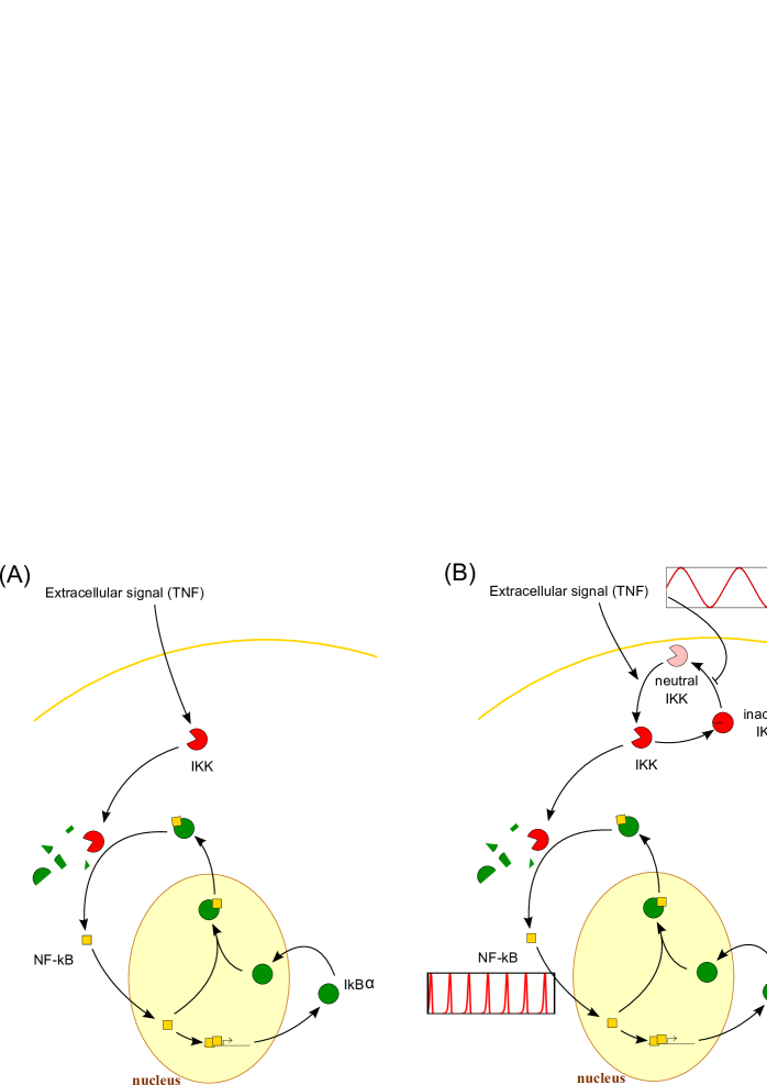
Figure 1: (A) Schematic diagram of processes that form the core feedback loop controlling NF-kB oscillations in the model of [21]. Nuclear NF-kB activates transcription of IkB which sequesters NF-kB in the cytoplasm. IkB kinase (IKK), when activated by external signals like the tumor necrosis factor alpha (TNF), causes eventual targeted degradation of IkB when it is bound to NFkB. The released NF-kB is then transported into the nucleus, closing the feedback loop. By assuming that all complexes are in equilibrium, these processes can be represented by three differential equations governing the dynamics of nuclear NFkB, IkB mRNA and cytoplasmic IkB (see text). The external TNF signal’s effect is simply modelled by appropriate choice of the degradation rate of IkB. This is sufficient when examining only steady levels of TNF, as is the case in [21]. (B) However, when examining the effect of temporally varying TNF signals, this model has to be extended as shown to include the interaction between TNF and various forms of IKK. We follow the model of [23] which consists of three forms of IKK which inter-convert cyclically. TNF enhances the conversion of neutral to active IKK, while also inhibiting the conversion of inactive to neutral IKK. Only active IKK is able to cause degradation of IkB. These processes can be represented by two additional differential equations (see text).

Here, we investigate the possibility of controlling the frequency of ultradian cellular oscillators by synchronizing them to external oscillations. Two important ultradian oscillators in mammalian cells are triggered by external stresses. After DNA-damage, the tumor suppressor protein p53 has been observed to oscillate with a period of 4–5 hours [17, 18]. Secondly, inflammatory stresses have been found to lead to oscillatory behavior in the transcription factor NF-kB [15]. Bulk and single cell measurements after treatment with tumor necrosis factor (TNF) show distinct and sharp oscillations with a time period of 2–3 hours [14, 15].

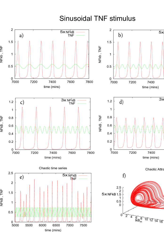
Figure 2: (A) Simulation with applied TNF amplitude $A=0.09$ and frequency $\nu=1/2.08~{}hr^{-1}$ (which is close to the reference frequency, $\nu_{0}=1/1.8~{}hr^{-1}$). Resultant NF-kB oscillations have the same frequency as the applied TNF signal, giving the 1/1 “tongue” in Fig. 3. (B) Simulation with $A=0.09$, $\nu=1/1.0~{}hr^{-1}$ (which is close to twice the reference frequency). Resultant NF-kB oscillations have twice the frequency of the applied TNF signal, giving the 1/2 “tongue” in Fig. 3. (C) Simulation with $A=0.09$, $\nu=1/0.83~{}hr^{-1}$ with initial conditions $N_{n}=1~{}\mu M,~{}I_{m}=0.5\mu M$ and all others zero $\mu M$. The NF-kB frequency synchronizes to be 1/3 of the applied frequency. (D) Simulation with $A=0.09$, $\nu=1/0.83~{}hr^{-1}$ identical to (C) except with different initial conditions where $N_{n}=0.1~{}\mu M,~{}I_{m}=0.5\mu M$ and all others zero $\mu M$. With these initial conditions, the NF-kB frequency synchronizes to 1/2 of the applied frequency. Thus, for this value of $A$ and $\nu$, we observe multiple stable synchronized states. (E) Simulation with $A=0.24$, $\nu=1/1.0~{}hr^{-1}$. At such large amplitudes chaotic oscillations are observed. (F) A plot of the trajectory of oscillations in the configuration space. The shape of the trajectory is quite typical of such chaotic oscillations and is known as a “strange attractor” [28].

In these two cases, oscillations are caused by a feedback loop which incorporates the formation of a complex between the transcription factor and an inhibitor (Mdm2 in the case of p53, and IkB$\alpha$ in the case of NF-kB). The complex formation induces an effective time delay through non-linear degradation which suffices to generate oscillations in the transcription factor and its inhibitor, out of phase with each other [19]. Those two feedback loops have been modeled both by applying explicit time delays [20] and by modelling the complex formation [19]. An elaborate model with 26 variables (mRNAs, proteins, complexes, etc.) for the NF-kB system was first formulated in Ref. [14]. Krishna et al. reduced this model to the core feedback loop by assuming that complexes were in equilibrium [21]. Fig. 1A shows a schematic representation of the resulting model that consists of three coupled non-linear differential equations:

$$\frac{dN_{n}}{dt}=k_{Nin}(N_{tot}-N_{n})\frac{K_{I}}{K_{I}+I}-k_{Iin}I\frac{N_{n}}{K_{N}+N_{n}}$$ (1)

$$\frac{dI_{m}}{dt}=k_{t}N_{n}^{2}-\gamma_{m}I_{m}$$ (2)

$$\frac{dI}{dt}=k_{tl}I_{m}-\alpha[IKK]_{a}(N_{tot}-N_{n})\frac{I}{K_{I}+I}$$ (3)

The triggering stimulus, e.g. TNF, acts by changing the level of active IkB kinase, $[IKK]_{a}$, which phosphorylates IkB, resulting eventually in its degradation. This degradation rate is one of the parameters of the model and Ref. [21] used different constant values of this parameter to represent different steady levels of the TNF stimulus. Default parameter values are given in Table 1. With these values and choosing $[IKK]_{a}=0.5~{}\mu M$ as in [21], one obtains sustained oscillations with a frequency $\nu=1/0.9~{}hr^{-1}$.

Here we wish to examine the effect of an oscillatory TNF stimulus on the system. The simplest possibility is to assume the degradation rate of IkB would oscillate identically to the TNF stimulus, and Ref. [22] showed that this could result in chaotic NF-kB oscillations. However, unlike steady levels of TNF, representing an oscillatory TNF signal by a similarly shaped oscillatory behavior of the IkB degradation rate is unjustifiable – non-linear interaction between TNF and IKK could well cause complex changes in the shape of the external signal as it is transduced. Therefore, we extended the model of Krishna et al [21] to include the circuit that transduces the TNF signal to the IKK concentration, as shown schematically in Fig. 1B. Ashall et al [23] have modelled this circuit in detail, and we add the two relevant differential equations from their model to the Krishna et al model:

$$\frac{d[IKK]_{a}}{dt}=k_{a}[TNF]([IKK]_{tot}-[IKK]_{a}-[IKK]_{i})-k_{i}[IKK]_{a}$$ (4)

$$\frac{d[IKK]_{i}}{dt}=k_{i}[IKK]_{a}-k_{p}[IKK]_{i}\frac{k_{A20}}{k_{A20}+[A20][TNF]}$$ (5)

This model assumes that there is a constant pool of IKK which is interconverted between different states – active, inactive and neutral. TNF increases the rate at which inactive IKK is made active, and it is only the active IKK which phosphorylates IkB and thereby affects the degradation rate of IkB$\alpha$. Ref. [23] constructed these equations so that the TNF signal can be represented by a dimensionless number between 0 (off) and 1 (on). We have used the parameters values from [23] (see Table 1) except for $N_{tot}$ and $[IKK]_{tot}$. Ref. [23] takes both $\sim 0.1\mu M$, whereas [21] uses $N_{tot}=1\mu M$. Here, we chose to keep $N_{tot}=1\mu M$ and varied $[IKK]_{tot}$ around 1$\mu M$, with $[TNF]$ fixed at 0.5, to find a value that gave sustained spiky oscillations with a frequency in the range 0.3–1 $hr^{-1}$. The model in [23] also includes another slow feedback via the molecule A20 as seen in the equations. For simplicity we ignore this feedback by keeping its concentration, $[A20]$, constant as this feedback loop mainly fine-tunes the shape of NF-kB response and “there is a range of constitutive A20 expression values that can functionally replace A20 negative feedback” [24]. As default values, we finally chose the combination of $[IKK]_{tot}=2~{}\mu M$ and $[A20]=0.0026~{}\mu M$. This results in sustained spiky oscillations of frequency $\nu_{0}\approx 1/1.8~{}hr^{-1}$ when $[TNF]$ is fixed at 0.5. Below, we show that with these parameter values oscillatory TNF stimuli in the model defined by equations (1)–(5) can produce both very organized responses – a multitude of synchronized states – as well as chaotic behavior. We have checked that our results are not qualitatively changed by perturbation of parameters around these default values, as long as the parameters result in sustained spiky oscillations when TNF is kept fixed at 0.5 (data not shown).

We examine both sinusoidal as well as square wave oscillation of TNF, and in each case vary the amplitude and frequency of the applied stimulus, while keeping the rest of the parameters of the model fixed. When TNF is sinusoidally varied with different frequencies around the average value 0.5, we observe that the NF-kB oscillation synchronizes in interesting ways to the applied TNF frequency. For example, when the applied frequency is close to the $\nu_{0}$, then the NF-kB oscillation synchronizes to have the same frequency as the external stimulus, as well as a constant phase difference between the maxima of TNF and NF-kB (see Fig 2a). Similarly, when the applied frequency is in a band close to $2\nu_{0}$, the NF-kB oscillation synchronizes to a period exactly twice the applied frequency (see Fig. 2b). A fundamental result of our investigation is that the NF-kB oscillations will stay completely synchronized even if the frequency of TNF oscillations is slightly diminished or slightly increased!. That is, the external TNF signal is able to ‘pull’ the frequency of the NF-kB oscillation towards a rational ratio with respect to the applied frequency. This is known as phase (or mode) locking [3]. As the amplitude of the applied oscillation increases, these bands of synchronization expand and the resulting shapes are called Arnold tongues [3]. Fig. 3a shows the Arnold tongues for the case where the TNF signal is sinusoidal, $[TNF](t)=0.5+Asin(2\pi\nu t)$, with varying frequency, $\nu$, and amplitude, $A$. Fig. 3b shows a similar diagram for the case when TNF is a square wave: $[TNF](t)=0.5+A[sign(sin(2\pi\nu t)+1]/2$. This protocol may be easier to realize experimentally than a sinusoidal one, and in fact shows broader Arnold tongues.

In principle, there is an Arnold tongue wherein NF-kB shows $p$ peaks for every $q$ peaks of TNF, for every rational number $p/q$ (where $p$ and $q$ are natural numbers). The width of each tongue starts off infinitely small when $A=0$, and expands smoothly as $A$ increases. Evidently, this cannot happen without tongues overlapping, and indeed such overlaps occur as soon as $A>0$. In general, in overlapping regions one expects to observe multistability, i.e. multiple synchronized states with different $p/q$ values will coexist, with different states being realized when different initial conditions are used. However, for small $A$, the states corresponding to small $p$ and $q$ numbers generally dominate the observed behavior. As $A$ is increased, these dominant states, such as 1/1 and 2/1, also start overlapping and then one can actually observe multistability (see Figs. 2c,d). As $A$ is increased further, and there are more and more overlaps, one can also encounter chaotic behavior as shown in Figs. 2e,f. The same behavior occurs for square wave oscillations of TNF (data not shown).

This complex behavior of the existence, growth and overlapping of Arnold tongues is observed in several very simple sets of nonlinear differential equations, such as circle maps and other return maps (we refer the reader to [3, 1, 8] for details). It has also been observed in a number of physical systems ranging from turbulent fluids, where synchronized states with rational numbers up to 83/79 haven been measured [4], quantum mechanical devices like Josephson junctions and semi-conductors [26, 8, 6, 25], crystals [7], and sliding charge-density waves [5]. Synchronization is known to occur in living systems, such as fireflies, and circadian clocks entrain to the day-night cycle [27]. However, to our knowledge such Arnold tongues have not been observed in vivo at a subcellular level.

Our work suggests that this kind of intricate synchronization could be observed in the NF-kB system, and also the p53-Mdm2 system as it has a very similar core feedback loop. More specifically, we predict that: (a) oscillations in NF-kB can be synchronized to TNF oscillations, (b) the bigger the amplitude, the stronger the synchronization (when amplitudes are relatively small), (c) the oscillations can in principle be synchronized to all rational ratios with respect to the applied frequency, but states with smaller $p$ and $q$ values will dominate, (d) if oscillations can be sustained for around a day, the states 1/2, 1/1 and 2/1 should be observable in practice, (e) when the amplitude of TNF oscillations is increased further, chaotic behavior will appear. Similar predictions could be made for the p53-Mdm2 system, controlled by external stimuli such as irradiation or exposure to DNA-damaging chemicals. If this basic synchronization technique works, we hope it could be developed into a tool to control inflammatory and apoptotic pathways and ultimately to regulate DNA repair, immune response and eventually cell fate.

(A,B)

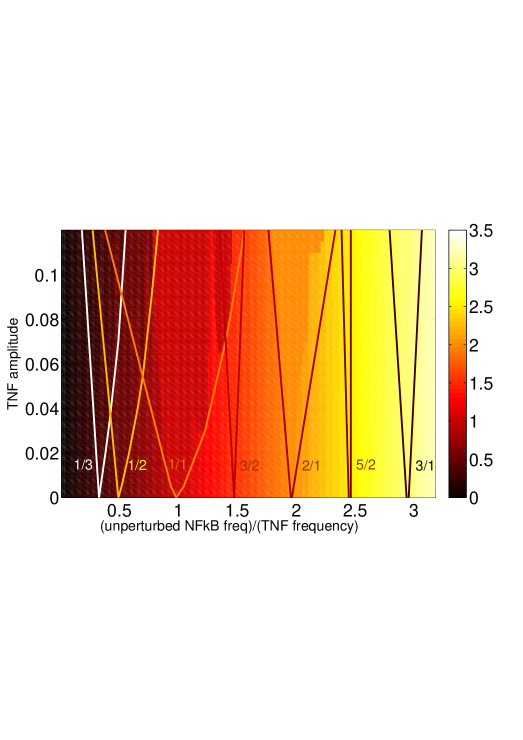
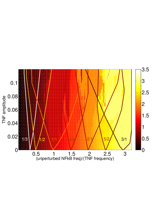
Figure 3: (A) Colors show the ratio of observed NF-kB frequency to the applied TNF frequency, as a function of TNF frequency and amplitude. The applied TNF signal is sinusoidal: $[TNF]=0.5+Asin(2\pi\nu t)$. The Arnold tongues corresponding to the states 1/3,1/2,1/1,3/2,2/1,5/2,3/1 are shown from left to right. For a tongue $p/q$, the boundary shown is the convex hull of points in the parameter space where the ratio of applied to observed frequency was within 0.5% of $p/q$. (B) Similar Arnold tongue diagram for the case where a square wave TNF signal is applied: $[TNF]=0.5+A[sign(sin(2\pi\nu t))+1]/2$.

Acknowledgement. This work was supported by the Danish National Science Foundation through the “Center for Models of Life”. We are grateful to Markus Covert for discussions on NF-kB oscillations and possible mode-locking in cells.

Parameter	Default value
$k_{Nin}$	5.4 min-1
$k_{Iin}$	0.018 min-1
$k_{t}$	1.03 ($\mu$M)-1.min-1
$k_{tl}$	0.24 min-1
$K_{I}$	0.035 $\mu$M
$K_{N}$	0.029 $\mu$M
$\gamma_{m}$	0.017 min-1
$\alpha$	1.05 ($\mu$M)-1.min-1
$N_{tot}$	1. $\mu$M
$k_{a}$	0.24 min-1
$k_{i}$	0.18 min-1
$k_{p}$	0.036 min-1
$k_{A20}$	0.0018 $\mu$M
$[IKK]_{tot}$	2.0 $\mu$M
$[A20]$	0.0026 $\mu$M

Table 1: Default values of parameters in the model. The first 9 are from Ref. [21] and the next 4 from Ref. [23]. $[IKK]_{tot}$ and $[A20]$ were chosen in order to obtain sustained spiky oscillations with frequency in the range 0.3–1 $hr^{-1}$ when $[TNF]$ is kept fixed at 0.5 (the actual frequency obtained with these values is $\nu_{0}=1/1.8~{}hr^{-1}$.)

References and Notes

- [1] A. Pikovsky, M. Rosenblum and J. Kurths, Synchronization: a universal concept in nonlinear sciences Cambridge University Press, Cambridge (2003).
- [2] A copy of the letter on this topic to the Royal Society of London appears in C. Huygens, in Ouevres Completes de Christian Huygens, edited by M. Nijhoff, Societe Hollandaise des Sciences, The Hague, The Netherlands (1893), Vol. 5, p. 246.
- [3] M.H. Jensen, P. Bak, and T. Bohr, Phys. Rev. Lett. 50, 1637 (1983); Phys. Rev. A 30, 1960 (1984).
- [4] J. Stavans, F. Heslot and A. Libchaber, Phys. Rev. Lett. 55, 596-599 (1985).
- [5] S. E. Brown, G. Mozurkewich and G. Gruner Phys. Rev. Lett. 52, 2277-2380 (1984).
- [6] E. G. Gwinn and R. M. Westervelt, Phys. Rev. Lett. 57 1060-1063 (1986).
- [7] S. Martin and W. Martienssen Phys. Rev. Lett. 56, 1522-1525 (1986).
- [8] W. J. Yeh, Da-Ren He, and Y. H. Kao Phys. Rev. Lett. 52, 480-480 (1984); Da-Ren He, W. J. Yeh, and Y. H. Kao Phys. Rev. B 31 1359-1373 (1985).
- [9] T. Y. Tsai et al Science 321 126 (2008).
- [10] Q. Thommen et al, PLoS Comput Biol 6(11) e1000990 (2010); B. Pfeuty, Q. Thommen, and M. Lefranc, Biophysical Journal 100, 2557 (2011).
- [11] L. Pedersen, S. Krishna and M.H. Jensen, PLoS ONE 6 e25550 (2011).
- [12] A. Goldbeter, Nature 420, 238-245 (2002)
- [13] B. O’Rourke, B.M. Ramza and E. Marban Science 265 962 (1994).
- [14] A. Hoffmann, A. Levchenko, M.L. Scott and D. Baltimore, Science 298, 1241 (2002).
- [15] D.E. Nelson et. al, Science 306, 704 (2004).
- [16] E.J. Waite, Y.M. Kershaw, F. Spiga and S.L. Lightman, Journal of Neuroendocrinology 21, 737 (2009).
- [17] N. Geva-Zatorsky, et al. Mol Sys Biol 2 2006.0033 (2006).
- [18] G. Lahav. Adv Exp Med Biol. 2008; 641 28 (2008).
- [19] B. Mengel, A. Hunziker, L. Pedersen, A. Trusina, M.H. Jensen and S. Krishna, Current Opinion in Genetics and Development 20, 656-664 (2010).
- [20] G. Tiana, K. Sneppen and M.H. Jensen, Europhys J B 29135 (2002).
- [21] S. Krishna, M.H. Jensen and K. Sneppen, Proc.Nat.Acad.Sci. 103, 10840 (2006).
- [22] J. Fonslet, K. Rud-Petersen, S. Krishna and M.H. Jensen, Int. Journ. Mod. Phys. B 21, 4083 (2007).
- [23] L. Ashall, et al Science 324, 242 (2009).
- [24] S. L. Werner, J. D. Kearns, V. Zadorozhnaya, et al. Genes Dev. 22, 2093 (2008).
- [25] A. Cumming and P. S. Linsay, Phys. Rev. Lett. 59, 1633 (1987).
- [26] P. Alstrom, M.H. Jensen and M.T. Levinsen, Physics Letters 103A 171-174 (1984).
- [27] G. Asher et al Cell 134, 317 (2008); G. Asher et al, Cell 142, 1–11 (2010).
- [28] S. Strogatz, ”Nonlinear Dynamics and Chaos”, Addison-Wesley, Reading (1994).