The role of damping for the driven anharmonic quantum oscillator

Abstract

For the model of a linearly driven quantum anharmonic oscillator, the role of damping is investigated. We compare the position of the stable points in phase space obtained from a classical analysis to the result of a quantum mechanical analysis. The solution of the full master equation shows that the stable points behave qualitatively similar to the classical solution but with small modifications. Both the quantum effects and additional effects of temperature can be described by renormalizing the damping.

In recent years, driven anharmonic oscillators have generated a large amount of interest because of their use as qubit readout devices (i.e., the Josephson bifurcation amplifier) [1, 2]. All these devices operate close to or in the quantum regime. There are two possible stable states in phase space, which can be distinguished by their respective amplitude and phase. Many studies have been performed on the transition between the stable states [3, 4, 5, 6, 7] and further effects like multiphoton resonances [8, 9] and dynamical tunneling [10, 11] make driven anharmonic oscillators an ideal model to study thermo-dynamics and quantum effects in a non-equilibrium system. Most bifurcation amplifiers are operated in the limit of strong damping to speed up the classical read-out process of the amplifier. In this paper, we define an equivalent to the classical stable state derived from a quantum master equation and discuss its position in phase space as a function of damping.

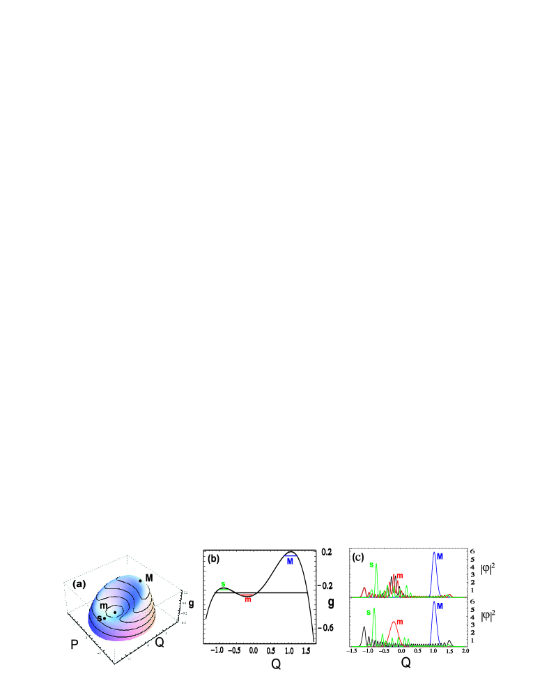
Figure 1: (a) A plot of the quasienergy $g$ in phase space. The extrema correspond to the two stable states, i.e., the high amplitude state (M) and the low amplitude state (m). The saddle point corresponds to an unstable state (s). The three kinds of classical orbits are also depicted by black closed curves. (b) A cut through the quasienergy potential $g$ for $P=0$. The quantum levels nearest to maximum (M), minimum (m) and saddle point (s) are shown in blue, red and green short lines respectively. Shown in long black line is the quantum level on the outer torus, which is close to and can be generate with level m. (c) Squared amplitude of the wave functions corresponding to quantum levels shown in Fig.1(b). We use the same colors and labels to distinguish them. The two subfigures correspond to different parameters, i.e., wave function on the outer torus is degenerate with the low amplitude state (top subfigure) and non-degenerate (bottom subfigure). We used $\lambda=0.027$ and $\beta=0.0341$ for this plot (degeneracy can be created by only minor changes of $\beta$).

The driven anharmonic oscillator is described by

$$H_{S}(t)=\frac{p^{2}}{2m}+\frac{m\Omega^{2}x^{2}}{2}-\gamma x^{4}+F(t)x,$$ (1)

where $F(t)=2F_{0}\cos(\nu t)$ stands for the external driving force. In the rotating frame and after a rotating wave approximation (RWA) the Hamiltonian reads

$$H=\Delta a^{\dagger}a+\chi{a^{\dagger}}a({a^{\dagger}}a+1)+f(a^{\dagger}+a).$$ (2)

Here, we have introduced the detuning between the oscillator’s natural frequency and the driving frequency $\Delta=\Omega-\nu$ , $\ \chi=-3\gamma\hbar/(2m^{2}\Omega^{3}),\ f=F_{0}/(\hbar\Omega)\sqrt{\hbar/(2m\Omega)}$. We then introduce the position operator $Q$ and momentum operator $P$ in the rotating frame $Q=\sqrt{{\lambda}/{2}}(a^{\dagger}+a),\ \ \ P=i\sqrt{{\lambda}/{2}}(a^{\dagger}-a),$ where $\lambda=-\chi/\Delta$ is the effective Planck constant. Finally, the scaled quasienergy Hamiltonian is defined as $H={\Delta^{2}}g/\chi,$ where

$$g=(Q^{2}+P^{2}-1)^{2}/4+\sqrt{\beta}Q.$$ (3)

Here, we have neglected some constant terms. Now all the properties of this system are dependent on one single quantity $\beta=-2f^{2}\chi/\Delta^{3}$. The quantum properties are contained in the commutation relation $[Q,P]=i\lambda$. The transition to the classical regime is equivalent to the limit $\lambda\rightarrow 0$. The dissipative environment is taken into account using the Lindblad master equation

$$\dot{{\rho}}(\tau)=-\frac{i}{\lambda}[H,{\rho}]+\eta\{(1+\bar{n}){\cal D}[a]{\rho}+\bar{n}{\cal D}[a^{\dagger}]{\rho}\},$$ (4)

where the Lindblad operator is defined through ${\cal D}[A]{\rho}\equiv A{\rho}A^{\dagger}-\frac{1}{2}\{A^{\dagger}A,{\rho}\}$, $\bar{n}$ is the Bose-Einstein distribution, and $\eta$ is the dimensionless damping strength [6, 12].

Let’s first discuss the classical dynamics of the driven Duffing oscillator in the weak-damping limit. For $0<\beta<4/27$, the Hamilton function exhibits three extrema in phase space, as indicated in Fig.1(a), i.e., a maximum M, a minimum m and a saddle point s. Without friction, there are three kinds of possible periodic orbits. They correspond to different isoenergetic sections of the Hamilton function. The orbits with an ear-shape around the maximum M form one group. Those circling the minimum m form another group. The third group consists of the orbits on the outer torus. One can calculate the explicit expressions of these orbits based on the classical equation of motion: $\partial_{t}Q=\partial_{P}g,\partial_{t}{P}=-\partial_{Q}g.$ In the vicinities of the extrema M and m the system is equivalent to an underdamped harmonic oscillator. Therefore, if damping is included the orbits nearby will shrink towards the extrema. As a result, they are stable points, corresponding to the oscillations with high and low amplitudes respectively. They are separated by a phase space barrier associated with the unstable saddle point s.

In the quantum limit, the classical orbits will be quantized into a series of discrete energy levels. They can be calculated by diagonalizing the scaled Hamiltonian (3), which results in a set of eigenvalues and eigenstates, i.e., $g|n\rangle=g_{n}|n\rangle$. In Fig.1(b) we show a cut through the quasienergy potential $g$ for $P=0$. The classically stable states are the extrema of the potential. The quantum levels corresponding to the three extrema are shown by colored short lines and labelled by M,m and s respectively. The black long line indicates one quantum level on the outer torus, which is close to and can be resonant with the level m. Fig.1(c) shows the quantum analogues (i.e., squared amplitude of the wave functions, $|\varphi|^{2}$) of the classical orbits corresponding to the quantum levels shown in Fig.1(b). We use the same colors and labels in each figures. In principle, the small amplitude state is coupled via tunnelling to states on the outer torus. If a state on the outer and inner torus are degenerate, the eigenstates are mixed states and this results in a large change of the degenerate wave functions (see the red and black curves in Fig.1(c)). However, one should note that in most of the relevant parameter regime the dynamics of the system is dominated by intra-well transitions [3, 5].

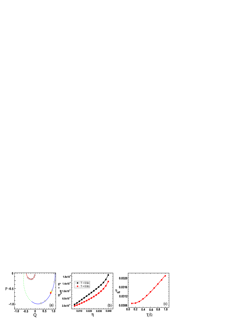
Figure 2: (a) Positions of the low amplitude state (red solid line), high amplitude state (blue solid line) and the unstable saddle point (green dashed line) from the solution of the classical equation of motion for finite damping and from the solution of the master equation (circles) respectively. The black empty circles represent zero temperature, while the yellow and red solid circles correspond to temperatures $T=2.0\Omega$ and $T=3.0\Omega$ respectively. (b) The difference between the effective damping $\eta_{\rm eff}$ and real quantum simulation damping $\eta$ at zero temperature (red solid circles) and $T=0.5\Omega$ (black solid squares) respectively. (c) The relationship between effective damping and temperature at fixed damping $\eta=0.03$. Other parameters are $\lambda=0.027$ and $\beta=0.12$.

As damping increases, the positions of the stable points in phase space will shift. We can find the classical solution for the stable points from the classical equation of motion including damping:$\ \dot{Q}=\partial g/\partial P-\eta Q,\ \dot{P}=-\partial g/\partial Q-\eta P$. For finite damping the system is classically bistable for $\beta^{(1)}<\beta<\beta^{(2)}$, with $\beta^{(1,2)}=2(1+9\eta^{2}\mp(1-3\eta^{2})^{3/2})/27$ [6]. In Fig.2(a), we plot the possible positions of the low amplitude state (red solid line), high amplitude state (blue solid line) and the unstable state (green dashed line) in phase space.

In order to describe the damping effects in the quantum regime, we turn to the master equation (4). We can also define a stable state using our master equation. At exactly zero temperature, it is possible to get an analytical expression for the stationary distribution in the so called P-representation [13, 14], which is one of several quasi-probability distributions [15, 16]. With the help of the P-representation, the exact analytical solution for the stationary density matrix for $\bar{n}=0$ can be obtained in the photon number representation (see Eq.(15) in Ref.[14]). We can diagonalize it and use its eigenstates as our basis. A diagonal representation will not only give us a clear physical picture of the dynamics of the system but also simplifies any numerical simulation.

To understand how our solution compares to the solution of the classical equation, we use the following procedure: (1) diagonalize the exact solution; (2) identify the eigenstates which correspond to the two stable states and calculate the expectation value of position and momentum (or amplitude and phase). An example for the results of such a calculation are the black empty circles in Fig.2(a); (3) compare the expectation values of the wave function with those expected from the classical equation of motion. Since the states are located on the same curve as the classical state we can assign each state a value $\eta_{\rm eff}$ that corresponds to the damping of the equivalent classical stable point.

Due to the finite effective Planck constant $\lambda$ used in this work, our results display some quantum effects. One is the disappearance of the small-amplitude state already for weaker damping than classically predicted. The reason is that near the bifurcation point, the low amplitude well is so shallow that the zero point energy exceeds the potential barrier. As a result, there is no quantum level in the vicinity of the minimum m. The situation is similar for the large-amplitude state if $\beta$ is small. Another quantum signature is the renormalization of damping, $\eta_{\rm eff}\neq\eta$. We show a comparison of $\eta$, as chosen for the master equation and the effective damping $\eta_{\rm eff}$ of the equivalent classical stable point in Fig.2(b). As $\lambda$ becomes smaller we find $\eta_{\rm eff}\approx\eta$ [6, 12].

The effect of temperature can be included in an exact numerical solution of the master equation. Then we again follow the steps outlined above and find that the eigenstates that diagonalize the matrix have average momenta and coordinates that fall on the curve of the classically stable states (see yellow and red solid circles in Fig.2(a)). We find that the temperature also introduces a weak renormalization of the damping $\eta$. We plot the difference, $\eta_{\rm eff}-\eta$, as function of $\eta$ in Fig.2(b) at a finite temperature (black solid squares in Fig.2(b)). We also show the renormalized damping as a function of $T$ for fixed $\eta$ in Fig.2(c). As one can see, there is a small quantum correction for $T=0$, and temperature has, as expected, no effect as long as $T\ll\Omega$. As temperature increases we get an additional small shift along the curve of the classically stable state. Generally we find that the states that diagonalize the density matrix at $T=0$ still remain an efficient diagonal basis up to $T\approx\Omega$.

References

References

- [1] Siddiqi I et al. 2004 Phys. Rev. Lett. 84 207002
- [2] Mallet F et al. 2009 Nature Physics 5 791
- [3] Dykman M I and Smelyansky V N 1988 Zh. Eksp. Teor. Fiz. 94 61
- [4] Vogel K and Risken H 1990 Phys. Rev. A 42 627
- [5] Marthaler M and Dykman M I 2006 Phys. Rev. A 73 042108
- [6] Dykman M I 2007 Phys. Rev. E 75 011101
- [7] Verso A and Ankerhold J 2010 Phys. Rev. E 82 05116
- [8] Dykman M I and Fistul M V 2005 Phys. Rev. B 71 140508(R)
- [9] Peano V and Thorwart M 2006 Chem. Phys. 322 135
- [10] Serban I and Wilhelm F K 2007 Phys. Rev. Lett. 99 137001
- [11] Marthaler M and Dykman M 2007 Phys. Rev. A 76 010102
- [12] Serban I, Dykman M I and Wilhelm F K 2010 Phys. Rev. A 81 022305
- [13] Drummond P D and Gardiner C W 1980 J. Phys. A: Math. Gen. 13 2353
- [14] Kheruntsyan K V 1999 J. Opt. B: Quantum Semiclass. Opt. 1 225
- [15] Carmichael H J 2001 Statistical Methods in Quantum Optics (Springer)
- [16] Vogel K and Risken H 1989 Phys. Rev. A 39 4675