All Two-Loop MHV Amplitudes in Multi-Regge Kinematics From Applied Symbology

Abstract

Recent progress on scattering amplitudes has benefited from the mathematical technology of symbols for efficiently handling the types of polylogarithm functions which frequently appear in multi-loop computations. The symbol for all two-loop MHV amplitudes in planar SYM theory is known, but explicit analytic formulas for the amplitudes are hard to come by except in special limits where things simplify, such as multi-Regge kinematics. By applying symbology we obtain a formula for the leading behavior of the imaginary part (the Mandelstam cut contribution) of this amplitude in multi-Regge kinematics for any number of gluons. Our result predicts a simple recursive structure which agrees with a direct BFKL computation carried out in a parallel publication.

I Introduction

Scattering amplitudes in gauge theories are complicated quantities even in relatively simple cases such as planar ${\cal N}=4$ supersymmetric Yang-Mills (SYM) theory and despite the dramatic recent improvements in our understanding of the mathematical structure of this theory. Some of this complication is unavoidable, since they depend non-trivially on many independent variables, and necessarily do so in terms of complicated functions: at weak coupling they can be expressed in terms of certain transcendental functions, and at strong coupling they compute minimal areas in anti-de Sitter space with prescribed boundary conditions (see Ref. Alday:2007hr ). Moreover at any coupling they apparently compute the expectation value of polygonal Wilson loops with lightlike edges, when suitably defined (see Refs. Alday:2007hr ; Drummond:2007aua ; Brandhuber:2007yx ; Mason:2010yk ; CaronHuot:2010ek ; Belitsky:2011zm ).

Pioneering progress towards taming at least some of this complexity has been made in Ref. Goncharov:2010jf by the introduction to the physics literature of the notion of the symbol of a generalized polylogarithm function (see Ref. Goncharov:2009 ). The symbol encapsulates much of the physically relevant information about an amplitude while simultaneously trivializing all of the functional identities which render it nearly impossible to work with polylogarithm functions directly. In particular the application of symbol technology (or “symbology”) enabled the determination of a relatively simple “one-line” analytic formula for the two-loop 6-particle MHV amplitude in Ref. Goncharov:2010jf (which had been evaluated numerically in Refs. Drummond:2007bm ; Bern:2008ap ; Drummond:2008aq and analytically in terms of several pages of polylogarithm functions thanks to the heroic effort of Refs. DelDuca:2009au ; DelDuca:2010zg ). Let us emphasize that symbology is a mathematical tool not restricted to SYM theory; see for example Ref. Manteuffel for a successful application to top quark pair production in QCD.

In recent work explicit results for the symbols of further amplitudes in SYM theory have started to accumulate in the literature, including the two-loop MHV amplitudes for all $n$ in Ref. CaronHuot:2011ky , the three-loop 6-particle MHV amplitude in Refs. Dixon:2011pw ; CaronHuot:2011kk , and the two-loop NMHV amplitudes for 6 and 7 particles respectively in Refs. Dixon:2011nj and CaronHuot:2011kk . Before proceeding let us note that that new techniques such as those developed in Refs. CaronHuot:2011kk ; Bullimore:2011kg seem to hold promise for generating much more data.

Unlike the case studied in Ref. Goncharov:2010jf , none of these amplitudes can be expressed in terms of the classical polylogarithm functions only. Despite this additional complexity it remains a very interesting open problem to find fully analytic formulas for these amplitudes in terms of generalized polylogarithms (see Ref. Duhr:2011zq for a possible algorithm towards this end).

Given this complexity we are led to study various limits in which the answers simplify and then to hope that more general lessons can be extracted from them. One way to simplify the problem is to consider the special case when the 4-momentum of each particle (or equivalently, all edges of the corresponding Wilson loop) lies in a common two-dimensional space. This has enabled some very simple results both at weak (see Refs. DelDuca:2010zp ; Heslop:2010kq ; Heslop:2011hv ; Gaiotto:2010fk ) and strong coupling (Ref. Alday:2009ga ).

Another limit in which scattering amplitudes simplify is in multi-Regge kinematics, a type of high-energy limit in which some kinematic invariants become much larger than others in a particular way described below. In the multi-Regge regime scattering amplitudes are expressed as an expansion both in powers of the coupling constant $g^{2}N_{c}$ and in powers of $\log(s/s_{0})$ where $s$ is some large kinematic invariant. The coefficients of this double series expansion are functions of the remaining finite kinematic invariants. The interested reader may consult Ref. Forshaw:1997dc for a pedagogical introduction. We will be working in the leading logarithm approximation, in which the effective summation parameter $g^{2}N_{c}\log(s/s_{0})$ is of order of unity. The choice of $s_{0}$ is then immaterial, and since all of the quantities we discuss will be dual conformally invariant and so depend only on cross-ratios (see Refs. Drummond:2007cf ; Drummond:2007au ) we will always be able to choose to express the expansion parameter as $\log(1-u)$ for some cross-ratio $u$ which is approaching unity.

In the Euclidean region where all energy invariants $s_{ij}$ are negative the multi-Regge behavior of MHV amplitudes is consistent with the BDS ansatz of Ref. Bern:2005iz to all orders (see Refs. Brower:2008nm ; Brower:2008ia ; DelDuca:2008jg ). However it was pointed out in Ref. Bartels:2008ce that in other regions the BDS ansatz is violated due to the presence of Mandelstam cuts. The difference between the actual MHV amplitude and the BDS ansatz is called the remainder function. In those other regions some energy invariants $s_{ij}$ become positive. This requires an analytic continuation whose effect at the level of cross-ratios is to multiply each one by some phase. This analytic continuation reveals the contribution from the Mandelstam cuts, which dominate over Regge poles in the remainder function, and behave at $L$-loop order like $\log^{L-1}(s_{ij}/s_{0})$, or $\log^{L-1}(1-u)$ when properly assembled into cross-ratios.

Let us note that the expansion of amplitudes in $\log(1-u)$ bears some superficial resemblance to the Wilson loop OPE expansion which has been studied quite fruitfully in a number of recent papers (see Refs. Alday:2010ku ; Gaiotto:2010fk ; Gaiotto:2011dt ; Sever:2011pc ; Sever:2011da ). In that case the expansion is taken in a variable $\tau$ which parameterizes the approach to a collinear limit. Despite the similarities, we emphasize that the two expansions are different in that they apply to different kinematic regions.

The discontinuities of MHV amplitudes in multi-Regge kinematics have been further studied in several recent papers (see for example Refs. Bartels:2008sc ; Schabinger:2009bb ; Lipatov:2010qf ; Lipatov:2010qg ; Lipatov:2010ad ; Bartels:2011xy ; Fadin:2011we ), and for example an all-loop prediction for the real part of the discontinuity in the case of 6 particles appeared in Ref. Bartels:2010tx . The multi-Regge behavior of amplitudes is of particular interest since it is expected (see for example Refs. Bartels:2008ce ; Bartels:2008sc ) to be universal for all gauge theories, thereby providing an interesting opportunity for applying results from SYM theory directly to QCD.

The main result of this paper is an analytic formula for the leading-log approximation to the Mandelstam cut contribution for all MHV amplitudes at two loops in a particular Mandelstam region (one corresponding to physical $2\to 2+(n-4)$ scattering). We obtain this result by extracting it from the symbols of the corresponding SYM theory super-Wilson loops constructed by Caron-Huot in Ref. CaronHuot:2011ky using an extended superspace. We find a very simple answer which is valid for an arbitrary number of particles and which is in perfect agreement with the result due to Bartels, Kormilitzin, Lipatov and Prygarin in the parallel publication Bartels:2011ge based on a direct BFKL computation (see Refs Lipatov:1976zz ; Kuraev:1976ge ; Kuraev:1977fs ; Balitsky:1978ic ). Since our SYM theory result implies a definite prediction for the corresponding quantity in QCD, this work provides a second application of symbology to LHC physics following the pioneering work of Robert Langdon.

In Sec. II we review a few important features of the well-studied $n=6$ particle amplitude before outlining the steps of our computation for general $n$ in Sec. III. The final symbological prediction for the amplitude is presented and discussed in Sec. IV.

II Invitation: The Six-Particle Amplitude

In order to set the stage for what follows let us briefly recall the story for the two-loop $n=6$-particle MHV remainder function in the multi-Regge kinematics, which has been studied in several recent papers. This function depends on three independent cross-ratios

$$u_{14}=\frac{(-s_{61})(-s_{34})}{(-s_{234})(-s_{345})},\qquad u_{25}=\frac{(-s_{12})(-s_{45})}{(-s_{123})(-s_{345})},\qquad u_{36}=\frac{(-s_{23})(-s_{56})}{(-s_{123})(-s_{234})}$$ (1)

where $s_{i\cdots}=(p_{i}+\cdots)^{2}$. Let $p_{1},p_{2}$ denote the incoming particles and $p_{3},p_{4},p_{5},p_{6}$ the outgoing particles. In the multi-Regge kinematics we have

$$|s_{12}|\gg|s_{345}|,|s_{123}|\gg|s_{34}|,|s_{45}|,|s_{56}|\gg|s_{234}|,|s_{23}|,|s_{61}|$$ (2)

and the cross-ratios approach

$$u_{25}\to 1^{-},\qquad u_{14},u_{36}\to 0^{+}$$ (3)

with $u_{14}/(1-u_{25})$ and $u_{36}/(1-u_{25})$ finite. It is conventional to parameterize the kinematics in terms of $u_{25}$ and two finite parameters $w,\bar{w}$ according to

$$u_{14}=(1-u_{25})\frac{w\bar{w}}{(1+w)(1+\bar{w})},\qquad u_{36}=(1-u_{25})\frac{1}{(1+w)(1+\bar{w})}.$$ (4)

Note that $w$ and $\bar{w}$ are not independent as they satisfy a quadratic equation with real coefficients, but they need not necessarily be complex conjugates.

To reach the Mandelstam region of interest for $2\to 2+2$ scattering we begin in the Euclidean region where all of the $s_{\cdots}$ invariants appearing above are negative and then ‘flip’ (that is, reverse the sign of the momentum of) particles 4 and 5. This leaves $u_{14}$ and $u_{36}$ unchanged while $u_{25}$ develops a phase

$$u_{25}\to e^{-2\pi i}u_{25}.$$ (5)

The analytically continued remainder function picks up an imaginary part from the Mandelstam cut contribution, whose behavior at two loops in multi-Regge kinematics with $u_{25}=1-\mathcal{O}(\epsilon)$ was shown in Ref. Lipatov:2010qg to be

$$R^{(2)}_{6}=\frac{i\pi\log\epsilon}{2}f_{6}(w,\bar{w})+\mathcal{O}(\epsilon^{0}),\qquad f_{6}(w,\bar{w})=\log|1+w|^{2}\log|1+1/w|^{2}$$ (6)

where $|1+w|^{2}$ is shorthand for $(1+w)(1+\bar{w})$, etc.

III Outline of the Calculation

Our goal is to generalize Eq. (6) by obtaining an explicit formula for the leading logarithmic behavior of the Mandelstam cut contribution to the two-loop $n$-particle MHV remainder function $R_{n}^{(2)}$ in a region corresponding to physical $2\to 2+(n-4)$ scattering; that is, the one in which all $n-4$ produced particles have their momenta flipped.

For $n>6$ we do not yet have at our disposal an explicit formula for the amplitude like the one in Ref. Goncharov:2010jf from which Eq. (6) was extracted. Instead we begin with the symbol $\mathcal{S}[R_{n}^{(2)}]$ of the two-loop MHV remainder functions in SYM theory derived in Ref. CaronHuot:2011ky for all $n$. Our calculation proceeds in two steps.

(1) The results of Ref. CaronHuot:2011ky are expressed in terms of momentum twistor variables (see Ref. Hodges:2010kq ). Although it in principle possible to reexpress everything in terms of cross-ratios (see appendix A) it seems much more natural and efficient for us to simply work out a parameterization of momentum twistors in multi-Regge kinematics, which we present in Section III.1. (A spinor helicity parameterization of the multi-Regge kinematics was used in Ref. DelDuca:1995zy .)

(2) Then we must isolate the appropriate imaginary part of the amplitude at the level of the symbol. As reviewed above, the imaginary terms in the physical region are generated by transformations of the form $u\to e^{i\phi}u$ acting on cross-ratios. In Section III.2 we show that for any $n$ only a single cross-ratio develops a non-zero phase in the physical region where particles $p_{4},\ldots,p_{n-1}$ have their momenta flipped. Furthermore we show that the (symbol of the) imaginary part of the amplitude in this region may be computed by simply isolating all terms in Ref. CaronHuot:2011ky which contain the momentum twistor invariant $\langle 123n\rangle$ in their first entry.

III.1 A Momentum Twistor Parameterization of Multi-Regge Kinematics

We consider $2\to n-2$ scattering, or the corresponding Wilson loop. It is convenient to use light-cone coordinates

$$p^{\pm}=p_{0}\pm p_{3},$$ (7)

and transverse coordinates $\vec{p}=(p_{1},p_{2})$ which we occasionally combine into the complex combination $\mathbf{p}=p^{1}+ip^{2}$. Then the norm and the scalar product are defined by

$$p^{2}=p^{+}p^{-}-\vec{p}^{2},\qquad p\cdot q=\frac{1}{2}p^{+}q^{-}+\frac{1}{2}p^{-}q^{+}-\vec{p}\cdot\vec{q}.$$ (8)

Without loss of generality we choose the incoming particles $p_{1}$ and $p_{2}$ to define the light-cone directions. In components this reads

$$p_{1}=(0,p_{1}^{-},\vec{0}),\qquad p_{2}=(p_{2}^{+},0,\vec{0}),\qquad p_{j}=(p_{j}^{+},p_{j}^{-},\vec{p}_{j}),$$ (9)

for $j=3,\dotsc,n$.

To parameterize the multi-Regge kinematics we begin with a generic configuration which we then deform by a parameter $\epsilon$ such that the multi-Regge region is approached in the limit $\epsilon\to 0$. The appropriate scaling of the momenta for $j=3,\dotsc,n$ is given by

$$p_{j}^{+}=\mathcal{O}(\epsilon^{-\frac{n+3}{2}+j}),\qquad p_{j}^{-}=\mathcal{O}(\epsilon^{\frac{n+3}{2}-j}),\qquad\mathbf{p}_{j}=\mathcal{O}(\epsilon^{0}),$$ (10)

which means that the produced particles are strongly ordered in rapidity ($\lvert p_{3}^{+}\rvert\gg\dotso\lvert p_{n-1}^{+}\rvert\gg\lvert p_{n}^{+}\rvert$ and $\lvert p_{3}^{-}\rvert\ll\dotso\ll\lvert p_{n-1}^{-}\rvert\ll\lvert p_{n}^{-}\rvert$).

We insert the explicit powers of $\epsilon$ necessary to implement Eq. (10) to parameterize the momenta for $j=3,\dotsc,n$ in spinor notation $p_{\alpha\dot{\alpha}}=p_{\mu}\sigma^{\mu}_{\alpha\dot{\alpha}}$ as

$$p_{j}=\begin{pmatrix}\epsilon^{j-\frac{n+3}{2}}p_{j}^{+}&{\bf p}_{j}\\ {\bf p}_{j}^{*}&\epsilon^{\frac{n+3}{2}-j}p_{j}^{-}\end{pmatrix},\qquad j=3,\ldots,n$$ (11)

in terms of the quantities $(p_{j}^{+},p_{j}^{-},\mathbf{p}_{j})$ which are held fixed, subject to the on-shell constraint $p_{j}^{+}p_{j}^{-}=|\mathbf{p}|^{2}$. Momentum conservation then determines

$$p_{1}=-\sum_{j=3}^{n}\begin{pmatrix}0&0\\ 0&\epsilon^{\frac{n+3}{2}-j}p_{j}^{-}\end{pmatrix},\qquad p_{2}=-\sum_{j=3}^{n}\begin{pmatrix}\epsilon^{j-\frac{n+3}{2}}p_{j}^{+}&0\\ 0&0\end{pmatrix}$$ (12)

and of course requires

$$\sum_{j=3}^{n}{\bf p}_{j}=0.$$ (13)

Now we choose spinors $\lambda_{\alpha}$, $\bar{\lambda}_{\dot{\alpha}}$ such that $p_{\alpha\dot{\alpha}}=\lambda_{\alpha}\bar{\lambda}_{\dot{\alpha}}$,

$$\lambda_{1}=\bar{\lambda}_{1}\simeq\begin{pmatrix}0\\ \sqrt{p_{1}^{-}}\epsilon^{-\frac{n-3}{4}}\end{pmatrix},\quad\lambda_{2}=\bar{\lambda}_{2}\simeq\begin{pmatrix}\sqrt{p_{2}^{+}}\epsilon^{-\frac{n-3}{4}}\\ 0\end{pmatrix},$$ (14)

$$\lambda_{j}=\begin{pmatrix}\sqrt{p_{j}^{+}}\epsilon^{-\frac{n}{4}+\frac{j}{2}-\frac{3}{4}}\\ \sqrt{p_{j}^{-}}\epsilon^{\frac{n}{4}-\frac{j}{2}+\frac{3}{4}}e^{i\phi_{j}}\end{pmatrix},\quad\bar{\lambda}_{j}=\begin{pmatrix}\sqrt{p_{j}^{+}}\epsilon^{-\frac{n}{4}+\frac{j}{2}-\frac{3}{4}}\\ \sqrt{p_{j}^{-}}\epsilon^{\frac{n}{4}-\frac{j}{2}+\frac{3}{4}}e^{-i\phi_{j}}\end{pmatrix},$$ (15)

where we have used the notation $\phi_{j}=\arg\mathbf{p}_{j}$. Note that for particles 1 and 2 it is sufficient to keep in Eq. (11) (and hence in Eq. (14)) the leading term as $\epsilon\to 0$.

Next we compute the dual variables $x_{i}$ defined by $p_{i}=x_{i}-x_{i-1}$ with the overall translation invariance fixed by choice $x_{n}=0$. These dual variables can be written in terms of momenta as $x_{j}=\sum_{k=1}^{j}p_{k}$. Using the expressions from Eq. (11) we have

$$x_{n}=\begin{pmatrix}0&0\\ 0&0\end{pmatrix},\quad x_{1}=\begin{pmatrix}0&0\\ 0&-\epsilon^{-\frac{n-3}{2}}\sum_{j=3}^{n}p_{j}^{-}\epsilon^{n-j}\end{pmatrix},$$ (16)

$$x_{j}=\begin{pmatrix}-\epsilon^{-\frac{n-3}{2}}\sum_{k=j+1}^{n}p_{k}^{+}\epsilon^{k-3}&\sum_{k=3}^{j}\mathbf{p}_{k}\\ \sum_{k=3}^{j}\mathbf{p}_{k}^{*}&-\epsilon^{-\frac{n-3}{2}}\sum_{k=j+1}^{n}p_{k}^{-}\epsilon^{n-k}\end{pmatrix}.$$ (17)

It may be tempting at this point to again keep in each individual entry only the leading term in the limit $\epsilon\to 0$. This however would make certain momentum-twistor invariants vanish identically. Since we need to keep track of the leading behavior of every independent invariant it is essential not to truncate the expansion of Eq. (16) prematurely, but rather to keep all orders of $\epsilon$ in the computation of the $x$’s.

With these ingredients we can compute the $\mu$ components of the twistors, which are defined by $\mu_{i\dot{\alpha}}=-\lambda_{i}^{\alpha}x_{i\alpha\dot{\alpha}}=\lambda_{i\alpha}\varepsilon^{\alpha\beta}x_{i\beta\dot{\alpha}}=\left(\lambda_{i}^{T}\cdot\varepsilon\cdot x_{i}\right)_{\dot{\alpha}}$. Again when computing $\mu_{i}$ it is imperative to avoid the temptation to keep only the leading term in $\epsilon$.

Finally once we have both $\lambda_{i}$ and $\mu_{i}$ we can assemble them into the momentum twistor $Z_{i}=(\lambda_{i\alpha},\mu_{i\dot{\alpha}})$. Note that the $Z$’s are projectively invariant, that is, for every non-vanishing $t$, $tZ$ is equivalent to $Z$. We use this projective invariance to set the first non-vanishing component of each $Z_{i}$ momentum to one.

In this manner we finally obtain the following momentum twistor parameterization of the multi-Regge kinematics:

$$Z_{n}=\begin{pmatrix}1\\ \epsilon^{-\frac{n-3}{2}}\alpha_{n}\\ 0\\ 0\end{pmatrix},\qquad Z_{1}=\begin{pmatrix}0\\ 1\\ 0\\ 0\end{pmatrix},\qquad Z_{2}=\begin{pmatrix}1\\ 0\\ 0\\ -\sum_{k=3}^{n}\alpha_{k}{\bf p}_{k}^{*}\epsilon^{\frac{n+3}{2}-k}\end{pmatrix},$$ (18)

$$Z_{j}=\begin{pmatrix}1\\ \epsilon^{\frac{n+3}{2}-j}\alpha_{j}\\ \sum_{k=3}^{j}{\bf p}_{k}+\alpha_{j}\sum_{k=j+1}^{n}\epsilon^{k-2}\mathbf{p}_{k}/\alpha_{k}\\ -\epsilon^{\frac{n+3}{2}-j}\alpha_{j}\sum_{k=3}^{j}{\bf p}_{k}^{*}-\sum_{k=j+1}^{n}\epsilon^{\frac{n+3}{2}-k}\alpha_{k}{\bf p}_{k}^{*}\end{pmatrix},\qquad j=3,\ldots,n-1$$ (19)

in terms of

$$\alpha_{j}=\sqrt{\frac{p_{j}^{-}{\bf p}_{j}}{p_{j}^{+}{\bf p}_{j}^{*}}}\,.$$ (20)

Armed with the $Z_{i}$ we are able to compute, in terms of the $\alpha$’s and $\mathbf{p}$’s, the leading $\epsilon\to 0$ behavior of all quantities appearing in the symbols derived in Ref. CaronHuot:2011ky . These include the elementary four-brackets

$$\langle ijkl\rangle=\det(Z_{i}\,Z_{j}\,Z_{k}\,Z_{l})$$ (21)

as well as the more complicated intersection forms

$$\langle ab(ijk)\cap(lmn)\rangle=\langle aijk\rangle\langle blmn\rangle-\langle bijk\rangle\langle almn\rangle,$$ (22)

$$\langle a(ij)(kl)(mn)\rangle=\langle iakl\rangle\langle jamn\rangle-\langle jakl\rangle\langle iamn\rangle.$$ (23)

III.2 Mandelstam Regions

As discussed in Ref. Bartels:2008ce for planar amplitudes in direct channels (when all energy invariants are positive) the Mandelstam cut contributions cancel in the multi-Regge kinematics. However, in other regions (Mandelstam regions) this does not happen, leading to the violation of a simple one-loop exponentiation ansatz suggested by the BDS ansatz. The Mandelstam regions are obtained by making some of the energy variables change their sign. For example for the $n=7$ particle amplitude one can consider the $2\to 5$ amplitude in a kinematic region analogous to the one shown in Fig. 1 with the three produced particles $4$, $5$ and $6$ being flipped as depicted in Fig. 2. The components of the flipped momenta change sign and the amplitude becomes kinematically non-planar (its projection onto the $(+-)$-plane cannot be drawn as a non-intersecting curve) while still being planar in color.

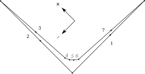
Figure 1: A heptagonal light-like Wilson loop projected onto the $(+,-)$-plane. The $j$-th edge vector is the momentum $p_{j}$ of particle $j$ in the corresponding scattering amplitude. In this region the remainder function vanishes in multi-Regge kinematics.

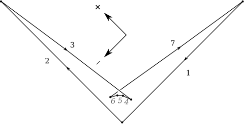
Figure 2: The Wilson loop of Fig. 1 with the edges corresponding to particles $4$, $5$ and $6$ being flipped to a positive energy region. In this region the Mandelstam cut gives a logarithmically divergent contribution to the remainder function in multi-Regge kinematics.

Our goal in this section is to understand how to isolate the imaginary part (the Mandelstam cut contribution) given only the symbol $\mathcal{S}[R^{(2)}_{n}]$ of the remainder function we are interested in. The analysis of this section therefore generalizes the discussion of Dixon:2011pw , in which the case $n=6$ was considered. For general $n$ there are $\frac{1}{2}n(n-5)$ multiplicatively independent cross-ratios of the type

$$u_{ij}=\frac{x_{i,j+1}^{2}x_{i+1,j}^{2}}{x_{ij}^{2}x_{i+1,j+1}^{2}},\qquad 2<|i-j|<n-2$$ (24)

where $x_{ij}=(x_{i}-x_{j})^{2}$ in terms of the dual variables $x_{i}$ reviewed above (only $3n-15$ of the $u_{ij}$ are algebraically independent in four dimensions due to Gram determinant constraints).

The symbol $\mathcal{S}[R_{n}^{(2)}]$ constructed in CaronHuot:2011ky contains, in its first entry, a larger population of objects called $u_{ijkl}$, but each of these can be uniquely expressed as a monomial in the $u_{ij}$. The multiplicative independence of the latter implies that there is a unique decomposition of the symbol as

$$\mathcal{S}[R_{n}^{(2)}]=\sum_{ij}u_{ij}\otimes U_{ij}$$ (25)

where each of the $U_{ij}$’s is a symbol of degree 3. Next we recall that the symbol of the discontinuity $\Delta_{u}f$ of a function $f$ in a given channel $u$ can be found by isolating the terms in its symbol $\mathcal{S}[f]$ with $u$ in the first entry and stripping off that entry. Multiplying the result of this procedure by $-2\pi i$ then yields the symbol $\mathcal{S}[\Delta_{u}f]$.

Hence all we need to do is determine which of the $u_{ij}$ develop a phase as particles 4 through $n-1$ are flipped. When we flip all $n-4$ produced particles in the $2\to n-2$ amplitude we find a discontinuity in $s_{4,\cdots,n-1}=x_{3,n-1}^{2}$. The invariant $x_{3,n-1}^{2}$ enters several different $u_{ij}$, each with various other $x$’s. However it is clear that only those invariants which span the $n-4$ produced particles (or a subset of them) change sign to positive, since the invariants which include the colliding particles $n,1,2,3$ do not change their energy components. Therefore amongst all of the $u_{ij}$ containing the invariant $x_{3,n-1}^{2}$, only

$$u_{2,n-1}=\frac{x_{2n}^{2}x_{3,n-1}^{2}}{x_{2,n-1}^{2}x_{3n}^{2}}=\frac{s_{3\cdots n}s_{4\cdots n-1}}{s_{3\cdots n-1}s_{4\cdots n}}$$ (26)

changes phase. Interestingly, this is also the single $u_{ij}$ which approaches $1$ most quickly in the multi-Regge kinematics: from the results obtained in the previous section it can be shown that

$$1-u_{2,n-1}=\mathcal{O}(\epsilon^{n-5}),$$ (27)

while all other cross-ratios that tend to unity do so no more quickly than $\mathcal{O}(\epsilon^{n-6})$.

Having concluded that only $u_{2,n-1}$ develops a phase in the Mandelstam region of interest, the symbol of the imaginary part of the remainder function in this region is given simply by

$$\mathcal{S}[R_{n}^{(2)}]=-2\pi i\,U_{2\,n{-}1}$$ (28)

in terms of the decomposition in Eq. (25). As a practical matter we note that it is trivial to read off $U_{2\,n{-}1}$ from the Mathematica file accompanying Ref. CaronHuot:2011ky because the four-bracket $\langle 123n\rangle$ serves as a unique signature for $u_{2,n{-}1}$. By this we mean that $\langle 123n\rangle$ appears only in the cross-ratio

$$u_{2,n{-}1}=\frac{\langle 123n\rangle\langle 34\,n{-}1\,n\rangle}{\langle 134n\rangle\langle 23\,n{-}1\,n\rangle}$$ (29)

and not in any other $u_{ij}$. Therefore in order to compute the coefficient $U_{2\,n{-}1}$ in the symbol it is sufficient to discard all terms in the symbol which do not have $\langle 123n\rangle$ in the first entry and simply strip off the leading $\langle 123n\rangle$ from those that do.

IV Results

At this stage all that remains is to take the $\epsilon\to 0$ limit of Eq. (28) evaluated on the momentum twistor parameterization constructed in Sec III.1. Such a limit may be safely taken at the level of the symbol by simply replacing each entry in the symbol by its leading order contribution at $\epsilon\to 0$.

IV.1 Consistency Checks

At $L$ loops we can only have a divergence like $\log^{L-1}(1-u)$, so it is expected that the two-loop amplitude $R_{n}^{(2)}$ should diverge only logarithmically

$$R_{n}^{(2)}\to-2\pi i\log\epsilon\ G^{(2)}_{n}+{\cal O}(\epsilon^{0})$$ (30)

where $G^{(2)}_{n}$ is a finite transcendentality two function. This expectation already demands two very non-trivial properties of $U_{2\,n{-}1}$ in multi-Regge kinematics. First of all it forbids from the symbol $\mathcal{S}[U_{2\,n{-}1}]$ any terms of the form

$$\epsilon\otimes\epsilon\otimes\epsilon,\qquad\epsilon\otimes\epsilon\otimes a,\qquad\epsilon\otimes a\otimes\epsilon,\qquad a\otimes\epsilon\otimes\epsilon$$ (31)

for any $a$, as these would correspond to $\log^{k}\epsilon$ divergences for $k>1$. Secondly, the factorization of Eq. (30) as a product of $\log\epsilon$ times a finite function requires that all terms in the symbol $U_{2\,n{-}1}$ with only a single $\epsilon$ must appear in the special form

$$\epsilon\otimes a\otimes b+a\otimes\epsilon\otimes b+a\otimes b\otimes\epsilon=\epsilon\operatorname{\sqcup\!\sqcup}a\otimes b$$ (32)

of a shuffle product of $\epsilon$ times some degree two symbol $a\otimes b$. After verifying the properties shown in Eqs. (31) and (32) this remaining degree two symbol is that of the function $G_{n}^{(2)}$ appearing in Eq. (30).

IV.2 The Main Formula

Our final result for the Mandelstam cut contribution to the two-loop $2\to 2+(n-4)$ MHV remainder function in the leading logarithm approximation is

$$R_{n}^{(2)}=\frac{i\pi\log\epsilon}{2}\sum_{i=4}^{n-2}\log\left\lvert\frac{\mathbf{x}_{23}\,\mathbf{x}_{i,n-1}}{\mathbf{x}_{2i}\,\mathbf{x}_{3,n-1}}\right\rvert^{2}\log\left\lvert\frac{\mathbf{x}_{2,n-1}\,\mathbf{x}_{3i}}{\mathbf{x}_{2i}\,\mathbf{x}_{3,n-1}}\right\rvert^{2}+\mathcal{O}(\epsilon^{0})$$ (33)

or equivalently

$$\frac{i\pi\log\epsilon}{2}\sum_{i=4}^{n-2}\log\left[\frac{|{\bf p}_{3}|^{2}|{\bf p}_{i+1}+\cdots+{\bf p}_{n-1}|^{2}}{|{\bf p}_{3}+\cdots+{\bf p}_{i}|^{2}|{\bf p}_{4}+\cdots+{\bf p}_{n-1}|^{2}}\right]\times\\ \log\left[\frac{|{\bf p}_{3}+\cdots+{\bf p}_{n-1}|^{2}|{\bf p}_{4}+\cdots+{\bf p}_{i}|^{2}}{|{\bf p}_{3}+\cdots+{\bf p}_{i}|^{2}|{\bf p}_{4}+\cdots+{\bf p}_{n-1}|^{2}}\right]+\mathcal{O}(\epsilon^{0}).$$ (34)

Strictly speaking this is a conjectured result based on explicit calculations we carried out for all values of $6\leq n\leq 17$. However, it is known that two-loop results for MHV scattering amplitudes and Wilson loops, when expressed in terms of a basis of integrals, have a form which stabilizes at a low number of points. This fact makes it clear that the form of the remainder function, and any of its limits, should have a similar property. Also, as discussed below, from knowledge of the symbol alone we cannot exclude the possibility of an additive term proportional to $\pi^{2}$ in these formulas; we omit such a term above because the direct BFKL calculation shows it to be absent Bartels:2011ge .

In order to facilitate comparison with a traditional BFKL calculation let us note that the large logarithm $-\log\epsilon$ may be traded for Mandelstam invariants via the relation

$$\frac{1}{2}\log(s_{12}/s_{n123})\simeq-\log\epsilon$$ (35)

which can be derived from the kinematics described in Sec. III.1.

Notice that the two cross-ratios inside the logarithms in Eq. (33) are related since they are obtained from the same four points: $2$, $3$, $i$ and $n-1$. This makes it is possible to rewrite the answer in the extremely simple recursive form

$$R_{n}^{(2)}=\frac{i\pi\log\epsilon}{2}\sum_{i=4}^{n-2}f_{6}(w_{i},\bar{w}_{i})+\mathcal{O}(\epsilon^{0}),$$ (36)

with

$$w_{i}=\frac{\mathbf{x}_{2,n-1}\,\mathbf{x}_{3i}}{\mathbf{x}_{23}\,\mathbf{x}_{i,n-1}}$$ (37)

and $f_{6}$ defined in Eq. (6). Note that for $n=6$, $w_{4}$ here is the same as the $w$ used in Eqs. (4) and (6).

As will be explained in the parallel publication Bartels:2011ge , the reason for this recursion is the fact that all produced particles are of the same helicity and the effective emission (Lipatov) vertices are built in such a way that adding the emission of one additional particle cancels the adjacent (purely transverse) propagator. Therefore at one and two loops the result can be easily obtained merely by redefining the transverse momenta of a bunch of the emitted particles that shrinks to a single emission point in the transverse space.

Let us now comment briefly on the symmetries of the answer. The remainder function has a dihedral symmetry acting on the particle labels. However, the multi-Regge limit treats some particles specially so the whole dihedral group is broken to a single non-trivial generator which fixes the vertex $x_{1}$. Under the action of this generator the vertices are permuted as $x_{2}\leftrightarrow x_{n}$, $x_{3}\leftrightarrow x_{n-1}$, etc. This action can also be written more concisely as $x_{i}\leftrightarrow x_{2-i\pmod{n}}$.

Under the action of this symmetry generator the vertex $x_{2}$ gets mapped to $x_{n}$ so it would seem that the cross-ratios $w_{i}$ get transformed into something entirely different. However, we should remember that for our multi-Regge kinematics $\mathbf{x}_{1}=\mathbf{x}_{2}=\mathbf{x}_{n}=0$. Keeping this in mind we have that the remaining symmetry generator acts as $w_{i}\to(w_{2-i\pmod{n}})^{-1}$. Since $f_{6}(w,\bar{w})=f_{6}(w^{-1},\bar{w}^{-1})$, we obtain that the result in Eq. (36) is invariant.

The Lorentz group is also broken by the choice of kinematics. The Lorentz transformations which preserve the multi-Regge kinematics act in the transverse space as $\mathbf{x}_{j}\to e^{i\psi}\mathbf{x}_{j}$. We also have translation symmetry $\mathbf{x}_{j}\to\mathbf{x}_{j}+\mathbf{a}$ and dilatations $\mathbf{x}_{j}\to\rho\mathbf{x}_{j}$. Finally, there is a parity transformation $\mathbf{x}_{j}\to\mathbf{x}_{j}^{*}$. The inversion transformation acts on the transversal coordinates as $\mathbf{x}_{j}\to\tfrac{\mathbf{x}_{j}}{x_{j}^{2}}$, but it does not act in a simple way on the cross-ratios in transverse coordinates.

When $\mathbf{x}_{j}\to\mathbf{x}_{3}$ or $\mathbf{x}_{j}\to\mathbf{x}_{n-1}$, the cross-ratios $w_{j}$ become infinite or vanish. However, we don’t expect any singularities to appear in these limits and, indeed, the answer we obtain has a smooth limit when $\mathbf{x}_{j}\to\mathbf{x}_{3}$ or $\mathbf{x}_{j}\to\mathbf{x}_{n-1}$.

IV.3 Beyond-the-Symbol Terms

The symbol only captures the leading functional transcendentality part of the answer, so it is important to ask if our result might be missing any “beyond-the-symbol” terms. Since we have a function of transcendentality degree two, any missing additive contributions ought to be of the form $\pi\times\log$ or $\pi^{2}$, multiplied by rational coefficients.

Under the assumption that only the transverse cross-ratios can appear as arguments of the logarithms, it is easy to see that we will always get unwanted singularities when $\mathbf{x}_{j}\to\mathbf{x}_{k}$ for some $j$ and $k$. So we we can exclude terms of the form $\pi\times\log$ where the arguments of the logarithms are transverse space cross-ratios. However, this argument cannot exclude the possibility of an additive constant proportional to $\pi^{2}$.

Appendix A Expressing Composite Four-Brackets in Terms of $u_{ij}$ Cross-Ratios

The two-loop $n$-point remainder function is parity even so it should be possible to express it in terms of familiar cross-ratios like $u_{ij}$ which are parity even. However, the form obtained by Caron-Huot in Ref. CaronHuot:2011ky is written in terms of momentum twistors and it is not immediately clear how to convert it to a form containing only $u_{ij}$-type cross-ratios. In this paper we have computed the multi-Regge kinematics directly from the momentum twistors, without converting to Mandelstam invariants $x_{ij}^{2}$ first.

We comment here on cross-ratios containing the most complicated type of composite four-brackets, $\langle ii+1(j-1jj+1)\cap(k-1kk+1)\rangle$. Consider in particular the quantities

$$x=\frac{\langle ii+1(j-1jj+1)\cap(k-1kk+1)\rangle}{\langle ij-1jj+1\rangle\langle i+1k-1kk+1\rangle},\quad\bar{x}=\frac{\langle i-1ii+1i+2\rangle\langle ii+1jk\rangle}{\langle i-1ii+1j\rangle\langle ii+1i+2k\rangle},$$ (38)

$$1-x=\frac{\langle ik-1kk+1\rangle\langle i+1j-1jj+1\rangle}{\langle ij-1jj+1\rangle\langle i+1k-1kk+1\rangle},\quad 1-\bar{x}=-\frac{\langle ii+1i+2j\rangle\langle ki-1ii+1\rangle}{\langle i-1ii+1j\rangle\langle ii+1i+2k\rangle},$$ (39)

where the bar means parity conjugate. Recall that parity conjugation in momentum twistor space is defined by

$$Z_{i}\to\frac{Z_{i-1}\wedge Z_{i}\wedge Z_{i+1}}{\langle i-1i\rangle\langle ii+1\rangle}$$ (40)

where the denominator involves the spinor helicity product $\langle i,j\rangle=\varepsilon_{\alpha\beta}\lambda_{i}^{\alpha}\lambda_{j}^{\beta}$. Note that in our conventions we have

$$x_{ij}^{2}=\frac{\langle ii+1jj+1\rangle}{\langle ii+1\rangle\langle jj+1\rangle}.$$ (41)

Then using

$$\langle ii+1i+2j\rangle\langle i+1j-1jj+1\rangle=\\ \langle ii+1\rangle\langle i+1i+2\rangle\langle j-1j\rangle\langle jj+1\rangle(x_{i,j-1}^{2}x_{i+1,j}^{2}-x_{j-1,i+1}^{2}x_{ij}^{2})$$ (42)

and

$$\langle ii+1jk\rangle\langle ii+1(j-1jj+1)\cap(k-1kk+1)\rangle=\\ \langle ii+1\rangle^{2}\langle j-1j\rangle\langle jj+1\rangle\langle k-1k\rangle\langle kk+1\rangle(-x_{ij}^{2}x_{ik}^{2}x_{j-1,k-1}^{2}+x_{ij}^{2}x_{i,k-1}^{2}x_{j-1,k}^{2}+\\ x_{i,j-1}^{2}x_{ik}^{2}x_{j,k-1}^{2}-x_{i,j-1}^{2}x_{i,k-1}^{2}x_{jk}^{2})$$ (43)

we get the following system of equations

$$(1-x)(1-\bar{x}) =\frac{(x_{i,j-1}^{2}x_{i+1,j}^{2}-x_{i+1,j-1}^{2}x_{ij}^{2})(x_{i-1,k-1}^{2}x_{ik}^{2}-x_{i,k-1}^{2}x_{i-1,k}^{2})}{(x_{i-1,j-1}^{2}x_{ij}^{2}-x_{i-1,j}^{2}x_{i,j-1}^{2})(x_{i,k-1}^{2}x_{i+1,k}^{2}-x_{ik}^{2}x_{i+1,k-1}^{2})},$$ (44)

$$x\bar{x} =\frac{x_{i-1,i+1}^{2}(x_{ij}^{2}x_{i,k-1}^{2}x_{j-1,k}^{2}-x_{ij}^{2}x_{ik}^{2}x_{j-1,k-1}^{2}+x_{i,j-1}^{2}x_{ik}^{2}x_{j,k-1}^{2}-x_{i,j-1}^{2}x_{i,k-1}^{2}x_{jk}^{2})}{(x_{i-1,j-1}^{2}x_{ij}^{2}-x_{i-1,j}^{2}x_{i,j-1}^{2})(x_{i,k-1}^{2}x_{i+1,k}^{2}-x_{ik}^{2}x_{i+1,k-1}^{2})}.$$ (45)

which determine the cross-ratios $x$ and $\bar{x}$ explicitly in terms of the Mandelstam invariants $x_{ij}^{2}$. Of course, there is an ambiguity in solving this system of quadratic equations, but the remainder function should be independent on the choice of solution. It is easy to rewrite the above system in terms cross-ratios of type $u_{ij}$. Needless to say, however, the resulting expressions for $x,\bar{x}$ become very complicated.

References

- (1) L. F. Alday and J. M. Maldacena, “Gluon scattering amplitudes at strong coupling,” JHEP 0706, 064 (2007) [arXiv:0705.0303 [hep-th]].
- (2) G. P. Korchemsky, J. M. Drummond and E. Sokatchev, “Conformal properties of four-gluon planar amplitudes and Wilson loops,” Nucl. Phys. B 795, 385 (2008) [arXiv:0707.0243 [hep-th]].
- (3) A. Brandhuber, P. Heslop and G. Travaglini, “MHV Amplitudes in Super Yang-Mills and Wilson Loops,” Nucl. Phys. B 794, 231 (2008) [arXiv:0707.1153 [hep-th]].
- (4) L. J. Mason and D. Skinner, “The Complete Planar S-matrix of SYM as a Wilson Loop in Twistor Space,” JHEP 1012, 018 (2010) [arXiv:1009.2225 [hep-th]].
- (5) S. Caron-Huot, “Notes on the scattering amplitude/Wilson loop duality,” JHEP 1107, 058 (2011) [arXiv:1010.1167 [hep-th]].
- (6) A. V. Belitsky, G. P. Korchemsky and E. Sokatchev, “Are scattering amplitudes dual to super Wilson loops?,” Nucl. Phys. B 855, 333 (2012) [arXiv:1103.3008 [hep-th]].
- (7) A. B. Goncharov, M. Spradlin, C. Vergu and A. Volovich, “Classical Polylogarithms for Amplitudes and Wilson Loops,” Phys. Rev. Lett. 105, 151605 (2010) [arXiv:1006.5703 [hep-th]].
- (8) A. B. Goncharov, “A simple construction of Grassmannian polylogarithms,” arXiv:0908.2238 [math.AG]
- (9) J. M. Drummond, J. Henn, G. P. Korchemsky and E. Sokatchev, “The hexagon Wilson loop and the BDS ansatz for the six-gluon amplitude,” Phys. Lett. B 662, 456 (2008) [arXiv:0712.4138 [hep-th]].
- (10) Z. Bern, L. J. Dixon, D. A. Kosower, R. Roiban, M. Spradlin, C. Vergu and A. Volovich, “The Two-Loop Six-Gluon MHV Amplitude in Maximally Supersymmetric Yang-Mills Theory,” Phys. Rev. D 78, 045007 (2008) [arXiv:0803.1465 [hep-th]].
- (11) J. M. Drummond, J. Henn, G. P. Korchemsky and E. Sokatchev, “Hexagon Wilson loop = six-gluon MHV amplitude,” Nucl. Phys. B 815, 142 (2009) [arXiv:0803.1466 [hep-th]].
- (12) V. Del Duca, C. Duhr and V. A. Smirnov, “An Analytic Result for the Two-Loop Hexagon Wilson Loop in SYM,” JHEP 1003, 099 (2010) [arXiv:0911.5332 [hep-ph]].
- (13) V. Del Duca, C. Duhr and V. A. Smirnov, “The Two-Loop Hexagon Wilson Loop in SYM,” JHEP 1005, 084 (2010) [arXiv:1003.1702 [hep-th]].
- (14) Talk by A. Manteuffel at ACAT 2011, http://goo.gl/K1Kvl.
- (15) S. Caron-Huot, “Superconformal symmetry and two-loop amplitudes in planar super Yang-Mills,” JHEP 1112, 066 (2011) [arXiv:1105.5606 [hep-th]].
- (16) L. J. Dixon, J. M. Drummond and J. M. Henn, “Bootstrapping the three-loop hexagon,” JHEP 1111, 023 (2011) [arXiv:1108.4461 [hep-th]].
- (17) S. Caron-Huot and S. He, “Jumpstarting the all-loop S-matrix of planar super Yang-Mills,” arXiv:1112.1060 [hep-th].
- (18) L. J. Dixon, J. M. Drummond and J. M. Henn, “Analytic result for the two-loop six-point NMHV amplitude in super Yang-Mills theory,” JHEP 1201, 024 (2012) [arXiv:1111.1704 [hep-th]].
- (19) M. Bullimore and D. Skinner, “Descent equations for superamplitudes,” arXiv:1112.1056 [hep-th].
- (20) C. Duhr, H. Gangl and J. R. Rhodes, “From polygons and symbols to polylogarithmic functions,” arXiv:1110.0458 [math-ph].
- (21) V. Del Duca, C. Duhr and V. A. Smirnov, “A Two-Loop Octagon Wilson Loop in SYM,” JHEP 1009, 015 (2010) [arXiv:1006.4127 [hep-th]].
- (22) P. Heslop and V. V. Khoze, “Analytic Results for MHV Wilson Loops,” JHEP 1011, 035 (2010) [arXiv:1007.1805 [hep-th]].
- (23) P. Heslop and V. V. Khoze, “Wilson Loops @ 3-Loops in Special Kinematics,” JHEP 1111, 152 (2011) [arXiv:1109.0058 [hep-th]].
- (24) D. Gaiotto, J. Maldacena, A. Sever and P. Vieira, “Bootstrapping Null Polygon Wilson Loops,” JHEP 1103, 092 (2011) [arXiv:1010.5009 [hep-th]].
- (25) L. F. Alday and J. Maldacena, “Minimal surfaces in AdS and the eight-gluon scattering amplitude at strong coupling,” arXiv:0903.4707 [hep-th].
- (26) J. R. Forshaw and D. A. Ross, Cambridge Lect. Notes Phys. 9, 1 (1997).
- (27) J. M. Drummond, J. Henn, G. P. Korchemsky and E. Sokatchev, “On planar gluon amplitudes/Wilson loops duality,” Nucl. Phys. B 795, 52 (2008) [arXiv:0709.2368 [hep-th]].
- (28) J. M. Drummond, J. Henn, G. P. Korchemsky and E. Sokatchev, “Conformal Ward identities for Wilson loops and a test of the duality with gluon amplitudes,” Nucl. Phys. B 826, 337 (2010) [arXiv:0712.1223 [hep-th]].
- (29) Z. Bern, L. J. Dixon and V. A. Smirnov, “Iteration of planar amplitudes in maximally supersymmetric Yang-Mills theory at three loops and beyond,” Phys. Rev. D 72, 085001 (2005) [hep-th/0505205].
- (30) R. C. Brower, H. Nastase, H. J. Schnitzer and C. I. Tan, “Implications of multi-Regge limits for the Bern-Dixon-Smirnov conjecture,” Nucl. Phys. B 814, 293 (2009) [arXiv:0801.3891 [hep-th]].
- (31) R. C. Brower, H. Nastase, H. J. Schnitzer and C. I. Tan, “Analyticity for Multi-Regge Limits of the Bern-Dixon-Smirnov Amplitudes,” Nucl. Phys. B 822, 301 (2009) [arXiv:0809.1632 [hep-th]].
- (32) V. Del Duca, C. Duhr and E. W. N. Glover, “Iterated amplitudes in the high-energy limit,” JHEP 0812, 097 (2008) [arXiv:0809.1822 [hep-th]].
- (33) J. Bartels, L. N. Lipatov and A. Sabio Vera, “BFKL Pomeron, Reggeized gluons and Bern-Dixon-Smirnov amplitudes,” Phys. Rev. D 80, 045002 (2009) [arXiv:0802.2065 [hep-th]].
- (34) L. F. Alday, D. Gaiotto, J. Maldacena, A. Sever and P. Vieira, “An Operator Product Expansion for Polygonal null Wilson Loops,” JHEP 1104, 088 (2011) [arXiv:1006.2788 [hep-th]].
- (35) D. Gaiotto, J. Maldacena, A. Sever and P. Vieira, “Pulling the straps of polygons,” JHEP 1112, 011 (2011) [arXiv:1102.0062 [hep-th]].
- (36) A. Sever and P. Vieira, “Multichannel Conformal Blocks for Polygon Wilson Loops,” JHEP 1201, 070 (2012) [arXiv:1105.5748 [hep-th]].
- (37) A. Sever, P. Vieira and T. Wang, “OPE for Super Loops,” JHEP 1111, 051 (2011) [arXiv:1108.1575 [hep-th]].
- (38) J. Bartels, L. N. Lipatov and A. Sabio Vera, “ supersymmetric Yang Mills scattering amplitudes at high energies: the Regge cut contribution,” Eur. Phys. J. C 65, 587 (2010) [arXiv:0807.0894 [hep-th]].
- (39) R. M. Schabinger, “The Imaginary Part of the Super-Yang-Mills Two-Loop Six-Point MHV Amplitude in Multi-Regge Kinematics,” JHEP 0911, 108 (2009) [arXiv:0910.3933 [hep-th]].
- (40) L. N. Lipatov, “Analytic properties of high energy production amplitudes in SUSY,” arXiv:1008.1015 [hep-th].
- (41) L. N. Lipatov and A. Prygarin, “Mandelstam cuts and light-like Wilson loops in SUSY,” Phys. Rev. D 83, 045020 (2011) [arXiv:1008.1016 [hep-th]].
- (42) L. N. Lipatov and A. Prygarin, “BFKL approach and six-particle MHV amplitude in super Yang-Mills,” Phys. Rev. D 83, 125001 (2011) [arXiv:1011.2673 [hep-th]].
- (43) J. Bartels, L. N. Lipatov and A. Prygarin, “Collinear and Regge behavior of MHV amplitude in super Yang-Mills theory,” arXiv:1104.4709 [hep-th].
- (44) V. S. Fadin and L. N. Lipatov, “BFKL equation for the adjoint representation of the gauge group in the next-to-leading approximation at SUSY,” Phys. Lett. B 706, 470 (2012) [arXiv:1111.0782 [hep-th]].
- (45) J. Bartels, L. N. Lipatov and A. Prygarin, “MHV amplitude for gluon scattering in Regge limit,” Phys. Lett. B 705, 507 (2011) [arXiv:1012.3178 [hep-th]].
- (46) J. Bartels, A. Kormilitzin, L. N. Lipatov and A. Prygarin, “BFKL approach and MHV amplitude,” arXiv:1112.6366 [hep-th].
- (47) L. N. Lipatov, “Reggeization Of The Vector Meson And The Vacuum Singularity In Nonabelian Gauge Theories,” Sov. J. Nucl. Phys. 23, 338 (1976) [Yad. Fiz. 23, 642 (1976)].
- (48) E. A. Kuraev, L. N. Lipatov and V. S. Fadin, “Multi-Reggeon Processes In The Yang-Mills Theory,” Sov. Phys. JETP 44, 443 (1976) [Zh. Eksp. Teor. Fiz. 71, 840 (1976)].
- (49) E. A. Kuraev, L. N. Lipatov and V. S. Fadin, “The Pomeranchuk Singularity In Nonabelian Gauge Theories,” Sov. Phys. JETP 45, 199 (1977) [Zh. Eksp. Teor. Fiz. 72, 377 (1977)].
- (50) I. I. Balitsky and L. N. Lipatov, “The Pomeranchuk Singularity In Quantum Chromodynamics,” Sov. J. Nucl. Phys. 28, 822 (1978) [Yad. Fiz. 28, 1597 (1978)].
- (51) A. Hodges, “The box integrals in momentum-twistor geometry,” arXiv:1004.3323 [hep-th].
- (52) V. Del Duca, “Equivalence of the Parke-Taylor and the Fadin-Kuraev-Lipatov amplitudes in the high-energy limit,” Phys. Rev. D 52, 1527 (1995) [arXiv:hep-ph/9503340].