Constellations and multicontinued fractions: application to Eulerian triangulations

Abstract.

We consider the problem of enumerating planar constellations with two points at a prescribed distance. Our approach relies on a combinatorial correspondence between this family of constellations and the simpler family of rooted constellations, which we may formulate algebraically in terms of multicontinued fractions and generalized Hankel determinants. As an application, we provide a combinatorial derivation of the generating function of Eulerian triangulations with two points at a prescribed distance.

1. Introduction

From the initial work of Hurwitz (1891) about transitive ordered factorizations of the identity in the symmetric group, to the bijective approach of Bousquet-Mélou and Schaeffer (2000) and Bouttier et al. (2004), including the more algebraic approach of Goulden and Jackson (1997), constellations appear in many forms in different areas of combinatorics. We refer the reader to the book of Lando and Zvonkin (2004) for an extensive review of the variety of contexts in which constellations appear.

In this paper, we focus on the map point of view, and consider the problem of enumerating planar constellations with two points at a prescribed distance. In Bouttier et al. (2004), this problem has already been tackled by giving a bijection between this family of constellations and a family of decorated trees called mobiles, which results in recurrence equations that characterize the associate generating functions. Remarkably, these recurrence equations admit explicit solutions (Di Francesco, 2005, Section 6.7), reminiscent of integrable systems (see also Bouttier et al. (2003a) for the solutions of the equations corresponding to $2$-constellations). The motivation of our work is to explain combinatorially the form of these solutions. Following the approach of Bouttier and Guitter (2011), we exhibit a connection between our enumeration problem and the a priori simpler problem of counting rooted constellations. This connection relies on a decomposition involving some lattice paths, which we may rephrase in terms of “multicontinued fractions”, in the spirit of Flajolet (1980). Solving our enumeration problem amounts to finding unknown coefficients in such a multicontinued fraction, which can be done via a generalization of Hankel determinants. We illustrate this approach in the case of Eulerian triangulations, where we provide a combinatorial derivation of a formula found in Bouttier et al. (2003b) for the generating function of Eulerian triangulations with two points at prescribed distance. These objects are in bijection with “very-well-labeled trees with small labels”, see also (Bousquet-Mélou, 2006, Section 2.1). The next section presents in more detail our main results and the organization of the paper.

2. Definitions and main results

A planar map is a proper embedding of a connected graph into the sphere, where proper means that edges are smooth simple arcs which meet only at their endpoints. Two planar maps are identical if one of them can be mapped onto the other by a homeomorphism of the sphere preserving the orientation. A planar map is made of vertices, edges and faces. The degree of a vertex or face is the number of edges incident to it (counted with multiplicity). Following Bousquet-Mélou and Schaeffer (2000), we consider a particular class of planar maps called constellations, see Fig.1.

Definition 1.

For $p\in\ldbrack 2,\infty\ldbrack$, a ($p$-)constellation is a planar map whose faces are colored black or white in such a way that :

• adjacent faces have opposite colors,

• the degree of any black face is $p$,

• the degree of any white face is a multiple of $p$.

Each edge of a constellation receives a canonical orientation by requiring that the white face is on its right. It is easily seen that the length of each oriented cycle is a multiple of $p$, and that any two vertices are accessible from one another. A constellation is rooted if one of its edges is distinguished. The white root face and black root face are respectively the white and black faces incident to the root edge. The root degree is the degree of the white root face. A constellation is said to be pointed if it has a distinguished vertex. Note that, in a pointed rooted constellation, the pointed vertex is not necessarily incident to the root edge.

In this paper, we consider $p$-constellations subject to a control on white face degrees, i.e. for each positive integer $k$ we fix the number of white faces of degree $kp$. This amounts to considering multivariate generating functions of constellations depending on an infinite sequence of variables $(x_{k})_{k\geq 1}$, where $x_{k}$ is the weight per white face of degree $kp$ and the global weight of a constellation is the product of the weights of its white faces. Two families of constellation generating functions will be of interest here.

The first family is that of rooted constellations with a prescribed root degree. More precisely, for $n\geq 1$, let $F_{n}\equiv F_{n}(x_{1},x_{2},\ldots)$ denote the generating function of rooted $p$-constellations with root degree $np$. By convention, we do not attach a weight $x_{n}$ to the white foot face and we set $F_{0}=1$.

The second family is that of pointed rooted constellations with a bounded “distance” between the root edge and the pointed vertex. More precisely, in a pointed constellation, we say that a vertex $v$ is of type $j\in\mathbb{N}$ if $j$ is the minimal length of an oriented path from $v$ to the pointed vertex (due to the orientation, it is slightly inappropriate to think of $j$ as distance) and we say that an edge is of type $j\to j^{\prime}$ if its origin and endpoint are respectively of type $j$ and $j^{\prime}$. Then, for $i\geq 1$, let $V_{i}\equiv V_{i}(x_{1},x_{2},\ldots)$ denote the generating function of pointed rooted $p$-constellations where the root edge is of type $j\to j-1$ with $j\leq i$. Note that $V_{1}$ is the generating function for rooted constellations (since for $i=1$, the pointed vertex must be the endpoint of the root edge). Furthermore, we add a conventional term $1$ to $V_{i}$, for all $i\geq 1$.

The fundamental observation of this paper may be stated as:

Theorem 1.

The sequences $(F_{n})_{n\geq 0}$ and $(V_{i})_{i\geq 1}$ are related via the multicontinued fraction expansion

(1) $$\sum_{n\geq 0}F_{n}t^{n}=\cfrac{1}{1-t\displaystyle\prod_{i_{1}=1}^{p-1}\cfrac{V_{i_{1}}}{1-t\displaystyle\prod_{i_{2}=1}^{p-1}\cfrac{V_{i_{1}+i_{2}}}{1-t\displaystyle\prod_{i_{3}=1}^{p-1}\cfrac{V_{i_{1}+i_{2}+i_{3}}}{\ddots}}}}$$

In the case $p=2$, the r.h.s. of (1) reduces to an ordinary continued fraction (of Stieljes-type). This corresponds to the bipartite case discussed in (Bouttier and Guitter, 2011, Eq. (1.13)): indeed, $2$-constellations may be identified with bipartite planar maps upon “collapsing” the bivalent black faces into non-oriented edges.

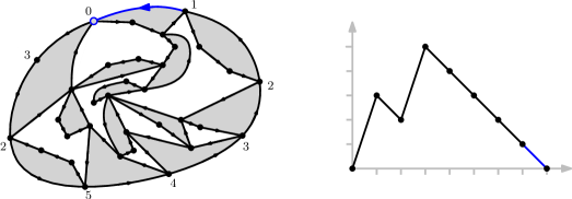
Figure 1. A rooted 4-constellation of $F_{2}$, with weight $x_{1}^{3}x_{2}^{4}$ and the 4-excursion associated to it.

In the spirit of the combinatorial theory of continued fractions initiated by Flajolet (1980), an alternate formulation of Theorem 1 may be given in terms of some lattice paths. We call $p$-path a lattice path on $\mathbb{Z}\times\mathbb{N}$ made of two types of steps: rises $(1,p-1)$ and falls $(1,-1)$. Note that a $p$-path starting from $(i_{0},j_{0})$ only visits vertices $(i,j)$ with $i+j\equiv i_{0}+j_{0}\mod p$. A $p$-excursion of length $np$ is a $p$-path that starts at $(0,0)$ and ends at $(np,0)$. It is well-known that such $p$-excursions are in one-to-one correspondence with $p$-ary rooted plane trees with $n$ nodes, in number $\frac{1}{np+1}\binom{np+1}{n}$. To each fall in a $p$-path, we attach a weight $V_{i}$ where $i$ is the starting height of the fall (i.e. the fall starts from $(j,i)$ for some $j$, and thus ends at $(j+1,i-1)$). We define the weight of a $p$-path as the product of the weights of its falls. As discussed in Section 3, the alternate formulation of Theorem 1 is then:

Theorem 2.

For all $n\geq 0$, $F_{n}$ is equal to the sum of weights of all $p$-excursions of length $np$.

We prove this theorem in Section 4. As an illustration, for $p=3$ and $n=1,2,3$, the equality reads

(2) $$\begin{split}F_{1}=V_{1}V_{2}&\\ F_{2}=V_{1}V_{2}&(V_{1}V_{2}+V_{2}V_{3}+V_{3}V_{4})\\ F_{3}=V_{1}V_{2}&(V_{1}^{2}V_{2}^{2}+2V_{1}V_{2}^{2}V_{3}+V_{2}^{2}V_{3}^{2}+2V_{1}V_{2}V_{3}V_{4}+2V_{2}V_{3}^{2}V_{4}+\\ &\phantom{(}V_{3}^{2}V_{4}^{2}+V_{2}V_{3}V_{4}V_{5}+V_{3}V_{4}^{2}V_{5}+V_{3}V_{4}V_{5}V_{6})\end{split}$$

We are now interested in inverting the relation (1), i.e. expressing $V_{i}$ in terms of the $F_{n}$’s. For $p=2$, this may be done using Hankel determinants (see below). However, as soon as $p\geq 3$, it is not difficult to see that knowing the sequence $(F_{n})_{n\geq 0}$ alone is not sufficient (for instance in (2) it appears that we have “twice as many unknowns as equations”).

We thus need some extra knowledge. A possible way is to consider, for all $n\geq 0$ and $r\geq 0$, the sum of weights of all $p$-paths that start at $(-r,r)$ and end at $(np,0)$, which we denote by $F_{n}^{(r)}$. Note that $F_{n}^{(0)}=F_{n}$ and, since a $p$-excursion necessarily starts with a rise, $F_{n}^{(p-1)}=F_{n+1}$. From now on, we restrict the values of $r$ to the interval $\ldbrack 0,p-2\rdbrack$. As will be discussed in Section 4, those $F_{n}^{(r)}$ have a natural interpretation in terms of constellations. Let us write down the first few $F_{n}^{(1)}$ for $p=3$:

(3) $$\begin{split}F_{0}^{(1)}&=V_{1}\\ F_{1}^{(1)}&=V_{1}V_{2}(V_{1}+V_{3})\\ F_{2}^{(1)}&=V_{1}V_{2}(V_{1}^{2}V_{2}+2V_{1}V_{2}V_{3}+V_{2}V_{3}^{2}+V_{1}V_{3}V_{4}+V_{3}^{2}V_{4}+V_{3}V_{4}V_{5})\\ \end{split}$$

It appears that, interlacing the equations in (3) and (2), we obtain a triangular system of equations for $V_{1},..,V_{6}$. This fact turns out to be general and, furthermore, the solution to our inverse problem is provided by the following formula, which we derive combinatorially in Section 3.

Theorem 3.

For $m\in\ldbrack 0,p-1\rdbrack$ and $n\in\mathbb{N}$, we have the determinantal identity

(4) $$H_{m;n}:=\det_{0\leq i,j\leq n}F_{q_{i+m}+j}^{(r_{i+m})}=\prod_{i=0}^{n}\prod_{j=1}^{ip+m}V_{j}$$

where, for $k\in\mathbb{N}$, $q_{k}$ and $r_{k}$ denote respectively the quotient and the remainder in the Euclidean division of $k$ by $p-1$, namely $q_{k}=\lfloor\frac{k}{p-1}\rfloor$ and $r_{k}=k-(p-1)q_{k}$.

Corollary 4.

For $m\in\ldbrack 0,p-1\rdbrack$ and $n\in\mathbb{N}$, we have

(5) $$V_{pn+m}=\begin{cases}\dfrac{H_{m;n}H_{m-1;n-1}}{H_{m;n-1}H_{m-1;n}}&\text{if }m\geq 1\\ \dfrac{H_{0;n}H_{p-1;n-2}}{H_{0;n-1}H_{p-1;n-1}}&\text{if }m=0\text{ and }n\geq 1.\end{cases}$$

with the convention $H_{m;-1}=1$.

Note that, for $p=2$, we recover the Hankel determinants: $H_{m;n}=\det_{0\leq i,j\leq n}F_{i+j+m}$ with $m=0$ or $1$. For $p=3$, the first few determinants read

(6) $$H_{0;0} =F_{0}^{(0)}=1 H_{1;0} =F_{0}^{(1)} H_{2;0} =F_{2}^{(0)}$$

$$H_{0;1} =\begin{array}[]{|cc|}F^{(0)}_{0}&F^{(0)}_{1}\\ F^{(1)}_{0}&F^{(1)}_{1}\end{array} H_{1;1} =\begin{array}[]{|cc|}F^{(1)}_{0}&F^{(1)}_{1}\\ F^{(0)}_{1}&F^{(0)}_{2}\end{array} H_{2;1} =\begin{array}[]{|cc|}F^{(0)}_{1}&F^{(0)}_{2}\\ F^{(1)}_{1}&F^{(1)}_{2}\end{array}$$

$$H_{0;2} =\begin{array}[]{|ccc|}F^{(0)}_{0}&F^{(0)}_{1}&F^{(0)}_{2}\\ F^{(1)}_{0}&F^{(1)}_{1}&F^{(1)}_{2}\\ F^{(0)}_{1}&F^{(0)}_{2}&F^{(0)}_{3}\\ \end{array}$$

and the reader may check, using (2) and (3), that those determinants are indeed monomials in the $V_{i}$’s, in agreement with (4). We conjecture that there is a simple relation between $H_{m;n}$ and $u_{(n+1)p+m}^{(p-2)}$ as defined at Equation (6.31) in Di Francesco (2005), so that Equation (6.30) ibid. amounts to Corollary 4.

In this paper, we present a simple application of Theorem 3 to the case of Eulerian triangulations, namely 3-constellations where all the white faces are also triangular. This corresponds to specializing the generating functions defined above at the values $p=3$, $x_{1}=x$, $x_{k}=0$ for $k\geq 2$, where $x$ is a variable controlling the number of triangles. In this case, the sequence $(V_{i})_{i\geq 1}$ is known to satisfy the simple recurrence

(7) $$V_{i}=1+xV_{i}\left(V_{i-1}+V_{i+1}\right),\qquad i\geq 1,\ V_{0}=0,$$

see Bouttier et al. (2003b). Clearly, this equation fully determines $V_{i}$ as a power series in $x$. In the same reference, it was observed that the solution of this equation has a remarkably simple form

(8) $$V_{i}=V\frac{(1-y^{i})(1-y^{i+4})}{(1-y^{i+1})(1-y^{i+3})}.$$

where $V$ and $y$ are power series determined by the equations $V=1+2xV^{2}$, $y+y^{-1}=(xV)^{-1}-2$. So far, there was no combinatorial explanation for the form of Equation 8. Theorem 3 provides such an explanation. Let us introduce the Fibonacci polynomials defined as follows (Flajolet and Sedgewick, 2009, eq. (62), p.327)

(9) $$\varphi_{n+2}(z)=\varphi_{n+1}(z)-z\varphi_{n}(z),\qquad\varphi_{0}(z)=0,\qquad\varphi_{1}(z)=1,$$

which are reciprocals of Chebyshev polynomials of the second kind, i.e. they satisfy the relation

(10) $$\varphi_{n}\left(\frac{1}{y+y^{-1}+2}\right)=\frac{1-y^{n}}{(1-y)(1+y)^{n-1}}.$$

Then, Equation 8 results from the following proposition, which we prove in Section 5.

Proposition 5.

Let $p=3$, $x_{k}=x\delta_{k,1}$ for $k\geq 1$ and $V=\sum_{n=0}^{\infty}\frac{(2n)!}{n!(n+1)!}(2x)^{n}$. For all $n\geq 0$, we have

(11) $$\begin{split}H_{0;n-1}&=V^{n(3n-1)/2}\varphi_{3n+1}(xV)\\ H_{1;n-1}&=V^{n(3n+1)/2}\varphi_{3n+2}(xV)\\ (1-xV)H_{2;n-1}&=V^{n(3n+3)/2}\varphi_{3n+3}(xV).\end{split}$$

3. $p$-paths and multicontinued fractions

We consider multivariate generating functions for $p$-paths with, for all $i\geq 1$, a weight $V_{i}$ per fall starting from a height $i$. All results stated in this section will hold with $(V_{i})_{i\geq 1}$ a sequence of formal variables (i.e. its definition of Section 2 in terms of constellations is not needed). Recall that, for $n,r\geq 0$, $F_{n}^{(r)}$ is defined as the generating function of $p$-paths starting from $(-r,r)$ and ending at $(np,0)$. Let us add an extra weight $t$ per rise and sum over all lengths, to obtain the generating functions

(12) $$F^{(r)}(t;V_{1},V_{2},\ldots):=\sum_{n\geq 0}F_{n}^{(r)}t^{n}.$$

By elementary recursive decompositions of $p$-paths, we obtain the recursive equations

(13) $$F^{(r)}(t;V_{1},V_{2},\ldots)=\begin{cases}1+t\,F^{(p-1)}(t;V_{1},V_{2},\ldots)&\text{if $r=0$}\\ V_{r}\,F^{(0)}(t;V_{r+1},V_{r+2},\ldots)\,F^{(r-1)}(t;V_{1},V_{2},\ldots)&\text{if $r\geq 1$}.\end{cases}$$

(For $r=0$ we remove the first rise. For $r\geq 1$ we perform first-passage decomposition at height $r-1$.) We easily deduce that

(14) $$F^{(0)}(t;V_{1},V_{2},\ldots)=\frac{1}{1-t\prod_{i=1}^{p-1}V_{i}F_{n}^{(0)}(t;V_{i+1},V_{i+2},\ldots)}$$

By iterating this relation, we find that $F^{(0)}(t;V_{1},V_{2},\ldots)$ is equal to the multicontinued fraction on the r.h.s. of (1). This shows that Theorem 2 (established in Section 4) implies Theorem 1.

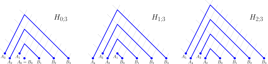
Figure 2. The unique configurations of non-intersecting lattice paths contributing respectively to $H_{0;3}$, $H_{1;3}$ and $H_{2;3}$ for $p=3$.

We now turn to the proof of Theorem 3, which is an application of the celebrated LGV lemma Lindström (1969); Gessel and Viennot (1989). We consider the weighted acyclic directed planar graph whose vertices are the $(k,l)\in\mathbb{Z}\times\mathbb{N}$ such that $k+l\equiv 0\mod p$, and whose edges are the rises $(k,l)\to(k+1,l+p-1)$, weighted $1$, and the falls $(k,l)\to(k+1,l-1)$, weighted $V_{l}$. For $n\in\mathbb{N}$, let $q_{n}$ and $r_{n}$ be respectively the quotient and the remainder in the Euclidean division of $k$ by $p-1$, and let

(15) $$A_{n}:=(-n-q_{n},r_{n})=(-pq_{n}-r_{n},r_{n}),\qquad B_{n}:=(np,0).$$

The generating function for paths from $A_{i}$ to $B_{j}$ ($i,j\geq 0$) is nothing but $F_{q_{i}+j}^{(r_{i})}$.

Theorem 3 then results from the LGV lemma and the following proposition, illustrated on Fig.2.

Proposition 6.

For $m\in\ldbrack 0,p-1\rdbrack$, there is a unique configuration of non-intersecting lattice paths connecting the sources $A_{m},A_{m+1},\ldots,A_{m+n}$ to the sinks $B_{0},B_{1},\ldots,B_{n}$: for $i\in\ldbrack 0,n\rdbrack$, the source $A_{m+i}$ is connected to the source $B_{i}$ via the highest possible path, passing through $(-m,m+ip)$. The weight of this configuration is $\prod_{i=0}^{n}\prod_{j=1}^{ip+m}V_{j}$.

The proof is left to the reader. For $p=2$ we recover the known combinatorial interpretation of Hankel determinants, see e.g. Viennot (1998).

4. Constellations, $p$-paths, and the slice decomposition

In this section, we establish Theorem 2 and related results.

Let us start with some definitions and notations. For $n\geq 1$, let $\mathcal{F}_{n}$ (resp. $\mathcal{F}^{\bullet}_{n}$) be the set of rooted (resp. pointed rooted) $p$-constellations with root degree $np$. The generating function of $\mathcal{F}_{n}$ is $F_{n}$ as defined in Section 2. Similarly, let $\mathcal{V}_{i}$ ($i\geq 1$) be the set of pointed rooted $p$-constellations whose root edge is of type $j\to j-1$ with $j\leq i$, to which we add a conventional “empty map” with weight $1$. The generating function of $\mathcal{V}_{i}$ is $V_{i}$.

A constellated path is a $p$-path such that, for all $i\geq 1$, an element of $\mathcal{V}_{i}$ is associated with each fall from height $i$. The weight of a constellated path is the product of the weights of its associated constellations. We shall consider constellated excursions and bridges, where a $p$-bridge of length $np$ is a $p$-path starting from $(0,j)$ and ending at $(np,j)$ from some $j\in\mathbb{N}$. Theorem 2 then follows from:

Proposition 7.

There is a weight-preserving bijection between $\mathcal{F}_{n}$ and the set of constellated excursions of length $np$. More generally, there is a weight-preserving bijection between $\mathcal{F}^{\bullet}_{n}\times\mathbb{N}$ and the set of constellated bridges of length $np$.

This bijection is a byproduct of the correspondence between constellations and mobiles introduced in Bouttier et al. (2004). Here we provide a direct construction, the so-called slice decomposition, extending the one given for $p=2$ by Bouttier and Guitter (2011).

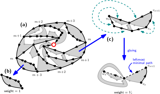
Figure 3. The decomposition of a rooted pointed $4$-constellation along leftmost minimal path into slices (a). Slice corresponding to edge $(m,m+3)$ are reduced to a black edge (b). Identifying the two sides of the boundary of a slice of an edge $(m,m-1)$ yields to a pointed-rooted constellation (c)

We start from a constellation $C\in\mathcal{F}^{\bullet}_{n}$, and a $\ell\in\mathbb{N}$ (whose role will be discussed at the very end). The white root face of $C$ forms a directed cycle which we denote by $(v_{0},v_{1},\ldots,v_{np-1},v_{np}=v_{0})$ where, say, $v_{0}$ is the endpoint of the root edge (hence $v_{np-1}$ is its origin).

Let $j_{s}$ be the type of $v_{s}$ (recall that the type of a vertex $v$ is the minimal length of an oriented path from $v$ to the pointed vertex), and let

(16) $$P:=((0,j_{0}+\ell),(1,j_{1}+\ell),\ldots,(np,j_{np}+\ell)).$$

We claim that $P$ is a $p$-bridge i.e. for all $s\in\ldbrack 0,np-1\rdbrack$,

(17) $$j_{s+1}-j_{s}\in\{-1,p-1\}.$$

Indeed, since $(v_{s},v_{s+1})$ is an oriented edge, we have $j_{s}\leq j_{s+1}+1$ by the definition of type. Furthermore, the black face incident to $(v_{s},v_{s+1})$ forms an oriented path of length $p-1$ from $v_{s+1}$ to $v_{s}$, hence $j_{s+1}\leq j_{s}+p-1$. Finally, since $p$ divides the length of any oriented cycle on $f$, we have $j_{s}\equiv j_{s+1}+1\mod p$, which concludes the proof of our claim. In particular, when $C$ is a rooted constellation that we point at the endpoint of the root edge, and $\ell=0$, then $P$ is a $p$-excursion.

Let us now explain how $P$ is constellated. Assume that the constellation $C$ is embedded in the plane with the white root face as outer face, and consider, for each $s$, the leftmost minimal (oriented) path from $v_{s}$ to the pointed vertex, where minimal refers to the length of the path. This family of paths leads to a decomposition of $C$ into connected components that we call slices, see Fig.3(a). A slice is associated with each edge $(v_{s},v_{s+1})$ incident to the white root face (thus with each step of $P$). More precisely, it is delimited by $(v_{s},v_{s+1})$ and the two paths starting from $v_{s}$ and $v_{s+1}$ (in general, those two paths merge before reaching the pointed vertex, and we remove their common part).

Observe that when $j_{s+1}=j_{s}+p-1$, the slice is reduced to a single black face (as the path starting from $v_{s+1}$ passes through $v_{s}$ after circumventing this face) with weight $1$, see Fig. 3 (b).

Let us now assume that $j_{s+1}=j_{s}-1$: we claim that the slice corresponds to an element of $\mathcal{V}_{j_{s}+\ell}$. Two cases may occur. If the path starting from $v_{s}$ passes through $v_{s+1}$, then the slice is empty, and corresponds to the empty map in $\mathcal{V}_{j_{s}+\ell}$. Otherwise, let $w_{s}$ be the vertex where the two paths starting from $v_{s}$ and $v_{s+1}$ merge. The boundary of the slice is therefore made of two (non-empty) oriented paths from $v_{s}$ to $w_{s}$ that do not meet except at their extremities. By construction those two paths have the same length: we may identify pairwise their edges, see Fig.3(c). This identification preserve the degrees of the white faces, hence the weights, and the orientations guarantee that the resulting map is a constellation $C_{s}$, which we root at $(v_{s},v_{s+1})$ and point at $w_{s}$. By construction, the identified paths form in $C_{s}$ the leftmost minimal path starting with the root edge and ending at the pointed vertex. Thus, in $C_{s}$ the root edge is of type $j^{\prime}_{s}\to j^{\prime}_{s}-1$, with $j^{\prime}_{s}\leq j_{s}\leq j_{s}+\ell$, so that $C_{s}\in\mathcal{V}_{j_{s}+\ell}$ as claimed. Note that since the pointed vertex of $C$ is incident to at least one white face, there is at least one $s$ such that $j^{\prime}_{s}=j_{s}$ i.e. $C_{s}\in\mathcal{V}_{j_{s}}\setminus\mathcal{V}_{j_{s}-1}$. This remark allows to characterize $\ell$ as the largest integer such that $P-(0,\ell)$ is still a constellated bridge.

In conclusion, the slice decomposition yields a constellated bridge. By following the steps in reverse order, it is clear how to reconstruct a pointed rooted constellation from a constellated bridge. By the above remark we also recover the integer $\ell$ and we may check that the correspondence is one-to-one (note that constellated bridges differing by a height shift yield the same constellation, but different values of $\ell$). Thereby we prove Proposition 7 and Theorem 2.

Let us now mention other byproducts of our construction.

Proposition 8.

For all $n\geq 0$ and $r\in\ldbrack 0,p-1\rdbrack$, $F_{n}^{(r)}$ is the generating function of rooted $p$-constellations with root degree $(n+1)p$ such that, if we denote by $(v_{0},v_{1},\ldots,v_{(n+1)p}=v_{0})$ the directed cycle corresponding to the white root face ($v_{0}$ being the endpoint of the root edge), then all the vertices $v_{1},v_{2},\ldots,v_{p-1-r}$ are bivalent.

Proof.

Apply the slice decomposition with $v_{0}$ as pointed vertex and $\ell=0$. The leftmost minimal path from $v_{1}$ to $v_{0}$ visits successively $v_{2},\ldots,v_{p-r}$, so that the constellated bridge starts with one rise followed by $p-1-r$ falls corresponding to empty slices. Removing those $p-r$ trivial steps, we obtain a constellated path with $np+r$ steps going from height $r$ to height $0$. ∎

Proposition 9 (Bouttier et al. (2004); Di Francesco (2005)).

Let $F_{n}^{(i-1;i)}$ be the generating function for constellated paths from $(0,i-1)$ to $(np-1,i)$. We have:

(18) $$V_{i}=1+V_{i}\sum_{n=1}^{\infty}x_{n}F_{n}^{(i-1;i)}$$

Proof.

Apply the slice decomposition to a (non-empty) map in $\mathcal{V}_{i}$. Taking $\ell=i-j$, where $j\to j-1$ is the type of the root edge, we obtain a constellated bridge of arbitrary length, starting at height $i-1$ and ending with a fall from height $i$, thus the factor $V_{i}$. The weight $x_{n}$ accounts for the white root face. ∎

Note the recursive nature of (18): $F_{n}^{(i-1;i)}$ is a polynomial in the $V_{j}$’s such that $|j-i|<(p-1)n$. In particular, for $i\to\infty$, $V_{i}$ converges (in a suitable topology) to $V$ the generating function of $\mathcal{V}=\bigcup_{i\geq 1}\mathcal{V}_{i}$, and $F_{n}^{(i-1;i)}\to\binom{np-1}{n}V^{n(p-1)-1}$. Hence $V$ satisfies the recursive equation

(19) $$V=1+\sum_{k=1}^{\infty}\binom{np-1}{n}x_{n}V^{n(p-1)}.$$

By the Lagrange inversion formula, we may obtain an explicit expression for the coefficients of $V$ (Bouttier, 2005, p.131), and recover the number of rooted constellations with a prescribed degree distribution (Bousquet-Mélou and Schaeffer, 2000, Theorem 2.3).

By extending the construction in (Bouttier and Guitter, 2011, Section 3.3), we may express the generating function $F_{n}$ in terms of $V$ as follows.

Proposition 10.

For $n\geq 0$, and $V$ the solution of (19), we have

(20) $$F_{n}=\frac{1}{np+1}\binom{np+1}{n}V^{n(p-1)+1}-\sum_{k\geq 1}\left(\sum_{j=0}\frac{jp+1}{np+1}\binom{np+1}{n-j}\binom{kp-1}{k+j}\right)x_{k}V^{(k+n)(p-1)}.$$

It would be interesting to have a similar formula for all $F_{n}^{(r)}$. We could then apply Theorem 3 and Corollary 4 and deduce a general expression for $V_{i}$. We may express $F_{n}^{(r)}$ in terms of $F_{n}$ using a Tutte-like decomposition (Bousquet-Mélou and Jehanne, 2006, Section 5.3), for instance for $p=3$ and $r=1$ we have

(21) $$F^{(1)}_{n}=\sum_{l\geq 1}x_{l}F_{n+l}+\sum_{i=0}^{n}F_{i}F_{n-i}.$$

Applying Proposition 10 yields in principle to an expression of $F_{n}^{(r)}$ in terms of $V$. In practice it seems to quickly become intractable, except in the case of Eulerian triangulations on which we focus next.

5. Application to Eulerian triangulations

We now specialize our formulas to the case of Eulerian triangulations, i.e. $p=3$ and $x_{k}=x\delta_{k,1}$. Note first that (18) reduces to (7), while (19) yields the simple equation $V=1+2xV^{2}$, hence $V$ is as in Proposition 5. Furthermore, (20) and (21) become respectively:

(22) $$F_{n}=\left(p^{(0)}_{n}\cdot(1-2xV)-p^{(3)}_{n-1}\cdot(xV)\right)V^{2n+1},\qquad F_{n}^{(1)}=xF_{n+1}+\sum_{i=0}^{n}F_{i}F_{n-i},$$

where we introduce the shorthand notation $p_{n}^{(r)}:=\frac{r+1}{3n+r+1}\binom{3n+r+1}{n}$, the number of $3$-paths from $(-r,r)$ to $(0,3n)$. By the relation $p_{n}^{(1)}=p_{n}^{(0)}+p_{n-1}^{(3)}$ (whose path interpretation is obvious), we may rewrite

(23) $$F_{n}=\left(p^{(0)}_{n}\cdot(1-xV)-p^{(1)}_{n}\cdot(xV)\right)V^{2n+1}.$$

Using this relation in the expression (22) for $F_{n}^{(1)}$, and using some summation formulas for the $p_{n}^{(r)}$’s (following from several classical path decompositions), we arrive at

(24) $$F_{n}^{(1)}=\left(p^{(1)}_{n}\cdot(1-xV)^{2}-p^{(0)}_{n+1}\cdot(xV)\right)V^{2n+2}.$$

We are now ready to substitute these formulas into the determinants $H_{n;m}$ ($m=0,1,2$) so as to prove Proposition 5. We will once again use the LGV lemma, to give another non-intersecting lattice path interpretation (NILP) of the $H_{n;m}$’s. Let us consider the same acyclic directed planar graph introduced in Section 3 for $p=3$ (i.e. the graph on which the $3$-paths live), but now with a uniform weight $1$ on every edge (rise or fall). Let $A_{n}$ and $B_{n}$ be as in (15) (for $p=3$), namely $A_{n}=(-\lfloor 3n/2\rfloor,r_{n})$ and $B_{n}=(3n,0)$, and let us extend the graph by adding the vertices

(25) $$A^{\prime}_{n}:=(-(3n+1)/2,-1),\qquad n\geq 0$$

and the special weighted edges

(26) $$\begin{cases}e_{2n}:=A^{\prime}_{2n}\to A_{2n}&\text{weighted }1\!-\!xV\\ \bar{e}_{2n}:=A^{\prime}_{2n}\to A_{2n+1}&\text{weighted }-\!xV\end{cases}\quad\begin{cases}e_{2n+1}:=A^{\prime}_{2n+1}\to A_{2n+1}&\text{weighted }(1\!-\!xV)^{2}\\ \bar{e}_{2n+1}:=A^{\prime}_{2n+1}\to A_{2n+2}&\text{weighted }-\!xV\end{cases}.$$

We readily see that the resulting graph is planar and, up to a factor $V^{2(i+j)+1}$ (resp. $V^{2(i+j+1)}$), that the generating function for paths from $A^{\prime}_{2i}$ (resp. $A^{\prime}_{2i+1}$) to $B_{j}$ ($i,j\geq 0$) is nothing but $F_{i+j}$ (resp. $F_{i+j}^{(1)}$). We may get rid of those extra factors by defining

(27) $$T_{3k+1}:=\frac{H_{0;k-1}}{V^{k(3k-1)/2}},\qquad T_{3k+2}:=\frac{H_{1;k-1}}{V^{k(3k+1)/2}},\qquad T_{3k+3}:=\frac{H_{2;k-1}(1-xV)}{V^{k(3k+3)/2}}.$$

and it follows from the LGV lemma that $T_{3k+1}$ (resp. $T_{3k+2}$ and $T_{3k+3}/(1-xV)$) is the generating function of NILP configurations from the sources $A^{\prime}_{0},\dots,A^{\prime}_{k-1}$ (resp. $A^{\prime}_{1},\dots,A^{\prime}_{k}$ and $A^{\prime}_{2},\dots,A^{\prime}_{k+1}$) to the sinks $B_{0},\ldots,B_{k-1}$. By convention, empty configurations (for $n=0$) receive the weight $1$ so that $T_{1}=T_{2}=1$ and $T_{3}=1-xV$. We claim that the $T_{n}$’s satisfy the recurrence relation

(28) $$T_{n+3}=(1-xV)T_{n+1}-xVT_{n}$$

and this is sufficient to prove that $T_{n}=\varphi_{n}(xV)$, since the Fibonacci polynomials with $z=xV$ satisfy the same recurrence and initial conditions, by (9). We prove (28) via a case-by-case analysis, depending on the residue of $n$ modulo 3. Here we only check the case $n=3k+1$, and leave the others cases to the reader (beware the extra $1-xV$ factor in $T_{3k+3}$). Consider a NILP configuration from $A^{\prime}_{0},\dots,A^{\prime}_{k}$ to $B_{0},\ldots,B_{k}$, as counted by $T_{3k+4}$. We first easily see that, for all $i$, the path $i$ (from $A^{\prime}_{i}$ to $B_{i}$) visits $(0,3i)$, and all the steps afterward are falls. We now distinguish whether the step before $(0,3k)$ on the uppermost path is a rise or a fall.

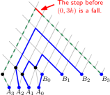
(a) If the last step before $(0,3k)$ is a rise, the upper-most path is deleted.

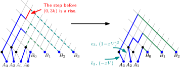
(b) If the last step before $(0,3k)$ is a fall, for each path, we replace the steps after the vertex $(-1,3i-1)$ by $3i-1$ falls

Figure 4. The decomposition of a configuration of $H_{0;4}$ into a configuration of $H_{0;3}$ (see 4(a)) or of $H_{1;3}$ (see 4(b)).

• If it is a fall, then all the preceding steps are rises, so that the path visits $A_{k+1}$ and passes through the special edge $\bar{e}_{k}$, thus has weight $-xV$. All the remaining paths form an unconstrained NILP configuration from the sources $A^{\prime}_{0},\ldots,A^{\prime}_{k-1}$ to the sinks $B_{0},\ldots,B_{k-1}$, with generating function $T_{3k+1}$. The global contribution of this case is $-xVT_{3k+1}$ (see Fig.4(a)).

• If it is a rise, i.e. the uppermost path visits $(-1,3k-1)$, then, by non-intersection, the path $i$ must visit $(-1,3i-1)$ for all $i\geq 1$, and the path $0$ is reduced to the special edge $e_{0}$, thus has weight $1-xV$. Remove the path $0$, and for each path $i\geq 1$, replace its steps after the vertex $(-1,3i-1)$ by $3i-1$ falls (see Fig.4): the resulting configuration is a NILP configuration from the sources $A^{\prime}_{1},\ldots,A^{\prime}_{k}$ to the sinks $B_{0},\ldots,B_{k-1}$, with generating function $T_{3k+2}$. Since the correspondence is one-to-one, the global contribution of this case is $-xVT_{3k+2}$ (see Fig.4(b)).

This shows that (28) holds with $n=3k+1$. Together with the cases $n=3k+2$ and $n=3k+3$, this concludes the proof of Proposition 5.

References

- Bousquet-Mélou (2006) M. Bousquet-Mélou. Limit laws for embedded trees: applications to the integrated superBrownian excursion. Random Structures and Algorithms, 29(4):475–523, 2006. arXiv:math/0501266 [math.CO].
- Bousquet-Mélou and Jehanne (2006) M. Bousquet-Mélou and A. Jehanne. Polynomial equations with one catalytic variable, algebraic series and map enumeration. Journal of Combinatorial Theory, Series B, 96(5):623–672, 2006. arXiv:math/0504018 [math.CO].
- Bousquet-Mélou and Schaeffer (2000) M. Bousquet-Mélou and G. Schaeffer. Enumeration of planar constellations. Advances in Applied Mathematics, 24(4):337–368, 2000.
- Bouttier (2005) J. Bouttier. Physique statistique des surfaces aléatoires et combinatoire bijective des cartes planaires. These, Université Pierre et Marie Curie - Paris VI, June 2005. URL http://tel.archives-ouvertes.fr/tel-00010651/en/.
- Bouttier and Guitter (2011) J. Bouttier and E. Guitter. Planar maps and continued fractions. Comm. Math. Phys., to appear, 2011. doi: 10.1007/s00220-011-1401-z. arXiv:1007.0419 [math.CO].
- Bouttier et al. (2003a) J. Bouttier, P. Di Francesco, and E. Guitter. Geodesic distance in planar graphs. Nuclear Physics B, 663(3):535 – 567, 2003a. arXiv:cond-mat/0303272 [cond-mat.stat-mech].
- Bouttier et al. (2003b) J. Bouttier, P. Di Francesco, and E. Guitter. Statistics of planar graphs viewed from a vertex: a study via labeled trees. Nuclear Physics B, 675(3):631–660, 2003b. arXiv:cond-mat/0307606 [cond-mat.stat-mech].
- Bouttier et al. (2004) J. Bouttier, P. Di Francesco, and E. Guitter. Planar maps as labeled mobiles. Electron. J. Combin, 11(1):R69, 2004. arXiv:math/0405099 [math.CO].
- Di Francesco (2005) P. Di Francesco. Geodesic distance in planar graphs: An integrable approach. The Ramanujan Journal, 10(2):153–186, 2005. arXiv:math/0506543 [math.CO].
- Flajolet (1980) P. Flajolet. Combinatorial aspects of continued fractions. Discrete Mathematics, 32(2):125–161, 1980.
- Flajolet and Sedgewick (2009) P. Flajolet and R. Sedgewick. Analytic combinatorics. Cambridge University Press, 2009.
- Gessel and Viennot (1989) I. Gessel and X. Viennot. Determinants, paths, and plane partitions. preprint, 132(197.15), 1989.
- Goulden and Jackson (1997) I. Goulden and D. Jackson. Transitive factorisations into transpositions and holomorphic mappings on the sphere. Proceedings of the American Mathematical Society, 125(1):51–60, 1997.
- Hurwitz (1891) A. Hurwitz. Über Riemann’sche Flächen mit gegebenen Verzweigungspunkten. Mathematische Annalen, 39(1):1–60, 1891.
- Lando and Zvonkin (2004) S. Lando and A. Zvonkin. Graphs on surfaces and their applications, volume 141. Springer Verlag, 2004.
- Lindström (1969) B. Lindström. Determinants on semilattices. Proc. Amer. Math. Soc., 20:207–208, 1969.
- Viennot (1998) X. G. Viennot. Une théorie combinatoire des polynômes orthogonaux. Notes de Cours, UQAM, Montréal, 1998. URL http://web.mac.com/xgviennot/Xavier_Viennot/polyn%C3%B4mes_orthogonaux.%html.