Neutrinos with Lorentz-violating operators of arbitrary dimension

Abstract

The behavior of fermions in the presence of Lorentz and CPT violation is studied. Allowing for operators of any mass dimension, we classify all Lorentz-violating terms in the quadratic Lagrange density for free fermions. The result is adapted to obtain the effective hamiltonian describing the propagation and mixing of three flavors of left-handed neutrinos in the presence of Lorentz violation involving operators of arbitrary mass dimension. A characterization of the neutrino coefficients for Lorentz violation is provided via a decomposition using spin-weighted spherical harmonics. The restriction of the general theory to various special cases is discussed, including among others the renormalizable limit, the massless scenario, flavor-blind and oscillation-free models, the diagonalizable case, and several isotropic limits. The formalism is combined with existing data on neutrino oscillations and kinematics to extract a variety of measures of coefficients for Lorentz and CPT violation. For oscillations, we use results from the short-baseline experiments LSND and MiniBooNE to obtain explicit sensitivities to effects from flavor-mixing Lorentz-violating operators up to mass dimension 10, and we present methods to analyze data from long-baseline experiments. For propagation, we use time-of-flight measurements from the supernova SN1987A and from a variety of experiments including MINOS and OPERA to constrain oscillation-free Lorentz-violating operators up to mass dimension 10, and we discuss constraints from threshold effects in meson decays and Čerenkov emission.

I Introduction

Nongravitational phenomena are well described by the minimal Standard Model (SM) of particle physics pdg . However, the existence of physics beyond the SM is established by the confirmed observation of neutrino oscillations, while the SM itself is believed to be a low-energy effective theory emerging from an underlying unified description of gravity and quantum physics at the Planck scale. Potential experimental signals exposing foundational Planck-scale physics are therefore of great interest but are challenging to identify. One proposed class of signals involves the breaking of Lorentz symmetry associated with tiny deviations from relativity ksp . In recent years, searches for Lorentz violation and related CPT violation have been performed with a wide range of systems and at impressive sensitivities tables .

Effective field theory can be used to describe Lorentz violation in realistic models at attainable energies kp . In this approach, CPT violation is associated with Lorentz violation owg . The comprehensive effective field theory incorporating the SM and General Relativity and characterizing general Lorentz violation is the Standard-Model Extension (SME) ck ; akgrav . Its Lagrange density behaves as a scalar density under observer transformations, so the SME action is coordinate independent. Each Lorentz-violating term is formed by contracting a Lorentz-violating operator of a given mass dimension $d$ with a controlling coefficient. The mass dimension $d$ provides a partial classification of the operators, and it offers a rough sense of the size of associated experimental effects.

In this work, we focus on Lorentz violation in neutrinos. The interferometric nature of neutrinos and their tiny apparent mass scale makes them natural probes for Planck-scale effects such as Lorentz and CPT violation. Various searches for Lorentz violation with neutrinos have achieved sensitivities to SME coefficients at levels comparable to Planck-suppressed effects, including ones by the LSND lsndlv , Super-Kamiokande (SK) sklv , MINOS minoslv1 ; minoslv2 , IceCube IceCube , and MiniBooNE MiniBooNElv collaborations, while evidence for superluminal neutrinos has recently been presented by the OPERA collaboration opera .

The introduction of neutrino coefficients for Lorentz and CPT violation ck has led to numerous efforts to understand their implications for neutrino behavior. The general effective hamiltonian describing neutrino propagation and mixing in the presence of Lorentz-violating operators of renormalizable dimension contains four types of coefficients km , leading to many novel effects that can be revealed in suitable experiments km-sb ; dkm . One interesting theoretical challenge is the construction of a global Lorentz-violating model describing all established neutrino behavior and perhaps also one or more of the known anomalies, without the two usual neutrino masses bicycle ; tandem ; bmw ; puma ; blmw . Many of the SME-based phenomenological studies of neutrino behavior focus on the special case of isotropic Lorentz violation in a preferred frame cg99 ; bpww ; bbm ; dg ; gl ; dgms ; dgpg ; gghm ; fk ; gktw ; dges ; jk ; rnknkm ; xm ; bgpg ; ba ; ym ; ag ; as ; bcgw ; ltz ; cmh , sometimes in the two-flavor limit. Several works treat anisotropic effects without lepton-number violation mp ; bef ; gl2 ; hmw ; bb ; akm ; bapion ; qm . Models also exist that incorporate nonconservation of lepton number, which leads to neutrino-antineutrino mixing scsk ; hmp ; hmp2 . The propagation of free neutrinos in the SME follows geodesics in a pseudo-Riemann-Finsler geometry finsler .

The primary goal of this paper is to extend available techniques for handling Lorentz violation in the neutrino sector to include operators of arbitrary mass dimension $d$. We are motivated partly by the notion that the usual SM represents the dominant component of a low-energy effective theory, with subdominant terms involving Lorentz violation given by the minimal SME with $d=3$ or $d=4$. In this picture, higher-order corrections involve Lorentz-violating operators of larger $d$, which are expected to grow in significance as energies increase and may thereby provide a link to the underlying theory kle . In some cases, such as supersymmetric Lorentz-violating theories susy , operators with $d>4$ can represent the dominant corrections to the SM. Similarly, in noncommutative quantum electrodynamics hayakawa , the action written in terms of the conventional fermion and photon fields contains only SME operators of dimension $d\geq 6$ chklo .

The analysis performed in this work has many parallels to the treatment for Lorentz-violating operators at arbitrary $d$ performed for the photon sector kmnonmin , and much of the methodology established for that work is applicable here. The formalism contains as a limiting case the earlier systematic investigation of neutrino operators of renormalizable dimension km and the corresponding SME-based studies of neutrino Lorentz violation mentioned above. However, the present work generalizes the existing treatment to include effects at leading order in both mass and Lorentz violation, uncovering novel Lorentz-violating effects involving neutrino helicity flip. It also incorporates as limiting cases studies of nonrenormalizable neutrino operators km ; amu ; jlm ; jc ; jp ; pbmp ; sehmr ; mmgls , including discussions of modified dispersion relations in the context of superluminal neutrinos ftlnu1 ; ftlnu2 ; ftlnu3 ; ftlnu4 ; jr ; re ; mrad ; dmpt ; jw ; kz ; gss ; aem ; cg ; lgm ; byyy ; cns ; ndhd ; jcjc ; afks ; mlm ; ssx ; frk ; aabp ; mr1 ; llmwz ; histy ; msch ; mmvv ; hllnq ; fbhl ; mr2 .

To achieve a reasonable scope while covering neutrino propagation and mixing in the presence of general Lorentz and CPT violation, we take the Lagrange density of interest to be quadratic in free fermion fields. Our methods and results are applicable to any type of fermion and hence are also relevant for other sectors of the SME. Implications of this and of possible interaction terms are considered elsewhere akmmnrint . In this work, our primary focus is the application to multiple generations of left-handed neutrinos. We obtain the effective hamiltonian describing neutrino propagation and mixing in the presence of Lorentz- and CPT-violating operators of arbitrary mass dimension. Since rotations form a subgroup of the Lorentz group, careful use of rotational properties often benefits experimental analyses, and so we develop a decomposition in spherical harmonics to characterize effects. We find that all Lorentz-violating features of neutrino propagation and mixing are determined by four sets of effective spherical coefficients for Lorentz violation, which can physically be distinguished by their Dirac or Majorana nature and by their CPT properties. Using this classification scheme, various limiting models can readily be identified and studied, and explicit measurements of coefficients for Lorentz violation can be extracted from observational and experimental data. Here, we use existing results from experiments on oscillations, times of flight, thresholds, and Čerenkov emission to tabulate measurements and maximal attained sensitivities for Lorentz-violating operators of mass dimensions $d\leq 10$. Many of our results represent the first available constraints on the corresponding Lorentz-violating effects.

The structure of this paper is as follows. The general quadratic action for a set of fermion fields in the presence of arbitrary Lorentz and CPT violation is presented in Sec. II. The specialization of this analysis to the neutrino sector, which allows for multiple flavors of left-handed neutrinos, is derived in Sec. III. The spherical decomposition of the effective hamiltonian for neutrino propagation is considered in Sec. IV. We discuss a variety of special cases in Sec. V, including the renormalizable limit, the massless scenario, flavor-blind and single-flavor models, the diagonalizable case, and isotropic models. The results are applied in Secs. VI and VII to extract numerous limits on coefficients for Lorentz violation from existing data on neutrino oscillations and propagation.

II Fermions

The construction of a realistic low-energy effective theory for fermions that is coordinate independent and describes general Lorentz violation can be achieved by adding appropriate terms to the conventional fermion Lagrange density. Each additional term is formed by contracting a coefficient for Lorentz violation with a tensor operator, and all possible terms are included kp ; ck ; akgrav . In this work we focus on noninteracting fermions, which corresponds to restricting Lorentz-violating terms in the action to fermion bilinears. The formalism presented in this section holds for arbitrary fermions, but our primary interest in subsequent sections lies in applications to neutrino physics for which chiral components are physically relevant.

Consider the case of $N$ spinor fields $\psi_{a}$, where $a$ ranges over $n$ spinor flavors $a=1,2,\ldots,N$. To allow for Majorana couplings in the construction, it is convenient to combine the $N$ spinors $\psi_{a}$ together with their charge conjugates $\psi^{C}_{a}=C\overline{\psi}{}^{T}_{a}$ into a $2N$-dimensional multiplet of spinors,

$$\Psi_{A}=\begin{pmatrix}\psi_{a}\\ \psi^{C}_{a}\end{pmatrix},$$ (1)

where $A$ ranges over $2N$ values. The redundancy in $\Psi$ implies that it obeys the relationship

$$\Psi^{C}=\mathcal{C}\Psi,\quad\mathcal{C}=\begin{pmatrix}0&1\\ 1&0\end{pmatrix},$$ (2)

where the $2N\times 2N$ matrix $\mathcal{C}$ is defined in terms of $N\times N$ blocks in flavor space.

In terms of the spinor $\Psi_{A}$, we can write the general Lagrange density incorporating Lorentz and CPT violation in the form

$$S = \int{\cal L}d^{4}x,$$

$${\cal L} = {\textstyle{1\over 2}}\overline{\Psi}{}_{A}(\gamma^{\mu}i\partial_{\mu}\delta_{AB}-M_{AB}+\widehat{\mathcal{Q}}_{AB})\Psi_{B}+{\rm h.c.}\quad$$ (3)

The first part of this expression generates the usual kinetic term, while the second part involves an arbitrary mass matrix $M_{AB}$. The third part contains the Lorentz-violating operator $\widehat{\mathcal{Q}}_{AB}$, which is a general $4\times 4$ matrix in spinor space and a $2N\times 2N$ matrix in flavor space that involves derivatives $i\partial_{\mu}$.

Since the effects from Lorentz violation are generically expected to be small, possibly arising as Planck-suppressed effects, it is reasonable to treat $\widehat{\mathcal{Q}}_{AB}$ as a perturbative contribution when necessary. This approach is adopted in the present work. In principle, the unperturbed theory could be taken as unconventional if desired. For example, some models of superluminal neutrinos adopt a kinetic term involving the replacement $i\gamma^{\mu}\partial_{\mu}\to i\gamma_{5}\gamma^{\mu}\partial_{\mu}$ ftlnu1 ; ftlnu2 ; ftlnu3 ; ftlnu4 ; jr ; re ; mrad ; dmpt ; jw ; kz . Models of this kind can be incorporated in the present formalism with a nonperturbative choice of $\widehat{\mathcal{Q}}_{AB}$.

The hermiticity of ${\cal L}$ implies that the general form of $M_{AB}$ can be written

$$M_{AB} = m_{AB}+im_{5AB}\gamma_{5},$$ (4)

where $m$ and $m_{5}$ are hermitian $2N\times 2N$ matrices. The relationship (2) implies the conditions

$$m=\mathcal{C}m^{T}\mathcal{C},\quad m_{5}=\mathcal{C}m_{5}^{T}\mathcal{C},$$ (5)

where the transpose acts in flavor space.

The operator $\widehat{\mathcal{Q}}_{AB}$ can in general depend on spacetime position, either in a prescribed way or through dynamical fields. For instance, explicit Lorentz violation occurs when $\widehat{\mathcal{Q}}_{AB}$ contains a fixed background with nontrival Lorentz properties, while spontaneous Lorentz violation can arise if $\widehat{\mathcal{Q}}_{AB}$ involves field variables with dynamics generating tensor vacuum values. An analysis incorporating spacetime dependence would be of interest but would be burdened by theoretical and experimental complexities beyond Lorentz violation, so it is advantageous to focus on operators that conserve energy and momentum. This can be assured by requiring the invariance of the action $S$ under spacetime translations, which is achieved when $\widehat{\mathcal{Q}}_{AB}$ is spacetime independent. For spontaneous Lorentz breaking, requiring invariance under spacetime translations implies neglecting soliton solutions, along with any massive or Nambu-Goldstone (NG) modes ng . The latter can be interpreted as the photon in Einstein-Maxwell theory akgrav ; bumblebee , as the graviton cardinal , or as a variety of other forces newforces .

We remark in passing that spacetime independence may be a natural feature of a model, or it may be a useful approximation describing dominant contributions or averaged effects from known or hypothesized forces in the vicinity of the Earth. Even Lorentz-invariant interactions typically generate effective Lorentz violation in this way. For example, couplings to a tiny and previously unknown Lorentz-invariant inverse-square force in the vicinity of the Earth would generate effective Lorentz-violating behavior described by the SME. This idea is the basis for some of the sharpest sensitivities obtained on torsion to date torsion and on some Lorentz-invariant effects from quantum gravity bs . Models for new Lorentz-invariant gravitational interactions are viable only if they are compatible with the numerous existing constraints for Lorentz violation tables . Experimental bounds on spacetime-independent $\widehat{\mathcal{Q}}_{AB}$ obtained in this work therefore also constrain Lorentz-invariant models involving neutrinos.

A decomposition of $\widehat{\mathcal{Q}}_{AB}$ permits the Lorentz-violating operators in ${\cal L}$ to be classified and enumerated. The spin part of $\widehat{\mathcal{Q}}_{AB}$ can be characterized by expanding in the basis of 16 Dirac matrices $\gamma_{I}$,

$$\widehat{\mathcal{Q}}_{AB} = \sum_{I}\widehat{\mathcal{Q}}_{AB}^{I}\gamma_{I}$$

$$\hskip-25.0pt=\widehat{\mathcal{S}}_{AB}+i\widehat{\mathcal{P}}_{AB}\gamma_{5}+\widehat{\mathcal{V}}_{AB}^{\mu}\gamma_{\mu}+\widehat{\mathcal{A}}_{AB}^{\mu}\gamma_{5}\gamma_{\mu}+{\textstyle{1\over 2}}\widehat{\mathcal{T}}_{AB}^{\mu\nu}\sigma_{\mu\nu},$$

where the $2N\times 2N$ derivative-dependent matrix operators $\widehat{\mathcal{Q}}_{AB}^{I}$ are hermitian in flavor space. The derivative dependence can be revealed by expressing each $\widehat{\mathcal{Q}}_{AB}^{I}$ as a sum of operators of definite mass dimension $d$,

$$\widehat{\mathcal{Q}}_{AB}^{I}=\sum_{d=3}^{\infty}\mathcal{Q}_{AB}^{(d)I\alpha_{1}\alpha_{2}\ldots\alpha_{d-3}}p_{\alpha_{1}}p_{\alpha_{2}}\ldots p_{\alpha_{d-3}},$$ (7)

where $p_{\mu}=i\partial_{\mu}$. Since each $\widehat{\mathcal{Q}}_{AB}^{I}$ has mass dimension one, the coefficients $\mathcal{Q}_{AB}^{(d)I\alpha_{1}\alpha_{2}\ldots\alpha_{d-3}}$ have mass dimension $4-d$. Following the discussion above, these coefficients can be taken as spacetime constants.

A useful refinement of the above decomposition involves first splitting $\widehat{\mathcal{Q}}_{AB}$ as

$$\gamma^{\nu}p_{\nu}\delta_{AB}-M_{AB}+\widehat{\mathcal{Q}}_{AB}=\widehat{\Gamma}^{\nu}_{AB}p_{\nu}-\widehat{M}_{AB},$$ (8)

in analogy to the usual split in the single-fermion limit of the minimal SME ck . The combination $\widehat{\Gamma}^{\nu}_{AB}p_{\nu}$ contains all operators of even mass dimension, while $\widehat{M}_{AB}$ contains all those of odd mass dimension. Expanding these combinations using Dirac matrices gives

$$\widehat{\Gamma}^{\nu}_{AB} = \gamma^{\nu}\delta_{AB}+\widehat{c}^{{\mu\nu}}_{AB}\gamma_{\mu}+\widehat{d}^{{\mu\nu}}_{AB}\gamma_{5}\gamma_{\mu}$$

$$+\widehat{e}^{\nu}_{AB}+i\widehat{f}^{\nu}_{AB}\gamma_{5}+{\textstyle{1\over 2}}\widehat{g}^{\kappa\lambda\nu}_{AB}\sigma_{\kappa\lambda},$$

$$\widehat{M}_{AB} = m_{AB}+im_{5AB}\gamma_{5}+\widehat{m}_{AB}+i\widehat{m}_{5}{}_{AB}\gamma_{5}$$ (9)

$$+\widehat{a}^{\mu}_{AB}\gamma_{\mu}+\widehat{b}^{\mu}_{AB}\gamma_{5}\gamma_{\mu}+{\textstyle{1\over 2}}\widehat{H}^{\mu\nu}_{AB}\sigma_{\mu\nu}.$$

The dimensionless operators $\widehat{c}^{{\mu\nu}}_{AB}$, $\widehat{d}^{{\mu\nu}}_{AB}$ are CPT even, while the dimensionless operators $\widehat{e}^{\mu}_{AB}$, $\widehat{f}^{\mu}_{AB}$, $\widehat{g}^{\mu\rho\nu}_{AB}$ are CPT odd. The remaining operators have mass dimension one, with $\widehat{m}_{AB}$, $\widehat{m}_{5}{}_{AB}$, $\widehat{H}^{\mu\nu}_{AB}$ being CPT even and $\widehat{a}^{\mu}_{AB}$, $\widehat{b}^{\mu}_{AB}$ being CPT odd. Note that all the operators in Eq. (9) have counterparts in the minimal SME except for $\widehat{m}_{AB}$ and $\widehat{m}_{5}{}_{AB}$, which contain only terms of nonrenormalizable dimension.

Since $\widehat{\Gamma}^{\nu}_{AB}$ appears contracted with $p_{\nu}$ in Eq. (8), the operators $\widehat{c}^{{\mu\nu}}_{AB}$, $\widehat{d}^{{\mu\nu}}_{AB}$, $\widehat{e}^{\mu}_{AB}$, $\widehat{f}^{\mu}_{AB}$, $\widehat{g}^{\mu\rho\nu}_{AB}$ are also automatically contracted with $p_{\nu}$. It is therefore natural and convenient to define the contracted operators

$$\widehat{c}^{\mu}_{AB} = \widehat{c}^{{\mu\nu}}_{AB}p_{\nu},\quad\widehat{d}^{\mu}_{AB}=\widehat{d}^{{\mu\nu}}_{AB}p_{\nu},$$

$$\widehat{e}_{AB} = \widehat{e}^{\nu}_{AB}p_{\nu},\quad\widehat{f}_{AB}=\widehat{f}^{\nu}_{AB}p_{\nu},\quad\widehat{g}^{\kappa\lambda}_{AB}=\widehat{g}^{\kappa\lambda\nu}_{AB}p_{\nu}.\qquad$$ (10)

The CPT properties of these contracted operators matches those of their counterparts in the minimal SME. Using this definition reveals the relationships

$$\widehat{\mathcal{S}}_{AB} = \widehat{e}_{AB}-\widehat{m}_{AB},\quad\widehat{\mathcal{P}}_{AB}=\widehat{f}_{AB}-\widehat{m}_{5}{}_{AB},$$

$$\widehat{\mathcal{V}}^{\mu}_{AB} = \widehat{c}^{\mu}_{AB}-\widehat{a}^{\mu}_{AB},\quad\widehat{\mathcal{A}}^{\mu}_{AB}=\widehat{d}^{\mu}_{AB}-\widehat{b}^{\mu}_{AB},$$

$$\widehat{\mathcal{T}}^{\mu\nu}_{AB} = \widehat{g}^{\mu\nu}_{AB}-\widehat{H}^{\mu\nu}_{AB}$$ (11)

between the expansions (LABEL:multiqhatsplit) and (8).

We can also take advantage of the property (2) to separate operators into Dirac and Majorana pieces. For each operator of mass dimension $d$ in $\widehat{\mathcal{Q}}_{AB}$, the property (2) yields the constraint

$$\widehat{\mathcal{Q}}=(-1)^{d-3}\mathcal{C}C\widehat{\mathcal{Q}}^{T}C^{-1}\mathcal{C},$$ (12)

where the transpose acts in both spinor and flavor spaces. This implies the conditions

$$\widehat{\mathcal{S}} = (-1)^{d+1}\mathcal{C}\widehat{\mathcal{S}}^{T}\mathcal{C},\quad\widehat{\mathcal{P}}=(-1)^{d+1}\mathcal{C}\widehat{\mathcal{P}}^{T}\mathcal{C},$$

$$\widehat{\mathcal{V}}^{\mu} = (-1)^{d}\mathcal{C}(\widehat{\mathcal{V}}^{\mu})^{T}\mathcal{C},\quad\widehat{\mathcal{A}}^{\mu}=(-1)^{d+1}\mathcal{C}(\widehat{\mathcal{A}}^{\mu})^{T}\mathcal{C},$$

$$\widehat{\mathcal{T}}^{\mu\nu} = (-1)^{d}\mathcal{C}(\widehat{\mathcal{T}}^{\mu\nu})^{T}\mathcal{C},$$ (13)

where now the transpose acts only in flavor space. Using these results, we can write the component operators $\widehat{\mathcal{Q}}^{I}_{AB}$ in terms of four $N\times N$ block matrices that can be designated as being of Dirac or Majorana type,

$$\widehat{\mathcal{S}} = \begin{pmatrix}\widehat{\mathcal{S}}_{D}&\widehat{\mathcal{S}}_{M}\\ \widehat{\mathcal{S}}_{M}^{\dagger}&(-1)^{d+1}\widehat{\mathcal{S}}_{D}^{T}\end{pmatrix},$$

$$\widehat{\mathcal{P}} = \begin{pmatrix}\widehat{\mathcal{P}}_{D}&\widehat{\mathcal{P}}_{M}\\ \widehat{\mathcal{P}}_{M}^{\dagger}&(-1)^{d+1}\widehat{\mathcal{P}}_{D}^{T}\end{pmatrix},$$

$$\widehat{\mathcal{V}}^{\mu} = \begin{pmatrix}\widehat{\mathcal{V}}^{\mu}_{D}&\widehat{\mathcal{V}}^{\mu}_{M}\\ (\widehat{\mathcal{V}}^{\mu}_{M})^{\dagger}&(-1)^{d}(\widehat{\mathcal{V}}^{\mu}_{D})^{T}\end{pmatrix},$$

$$\widehat{\mathcal{A}}^{\mu} = \begin{pmatrix}\widehat{\mathcal{A}}^{\mu}_{D}&\widehat{\mathcal{A}}^{\mu}_{M}\\ (\widehat{\mathcal{A}}^{\mu}_{M})^{\dagger}&(-1)^{d+1}(\widehat{\mathcal{A}}^{\mu}_{D})^{T}\end{pmatrix},$$

$$\widehat{\mathcal{T}}^{\mu\nu} = \begin{pmatrix}\widehat{\mathcal{T}}^{\mu\nu}_{D}&\widehat{\mathcal{T}}^{\mu\nu}_{M}\\ (\widehat{\mathcal{T}}^{\mu\nu}_{M})^{\dagger}&(-1)^{d}(\widehat{\mathcal{T}}^{\mu\nu}_{D})^{T}\end{pmatrix}.$$ (14)

In these expressions, all the Dirac-like matrices are hermitian in flavor space. Depending on the mass dimension, each Majorana matrix operator is either symmetric or antisymmetric in flavor space,

$$\widehat{\mathcal{S}}_{M} = (-1)^{d+1}\widehat{\mathcal{S}}_{M}^{T},\quad\widehat{\mathcal{P}}_{M}=(-1)^{d+1}\widehat{\mathcal{P}}_{M}^{T},$$

$$\widehat{\mathcal{V}}_{M}^{\mu} = (-1)^{d}(\widehat{\mathcal{V}}_{M}^{\mu})^{T},\quad\widehat{\mathcal{A}}_{M}^{\mu}=(-1)^{d+1}(\widehat{\mathcal{A}}_{M}^{\mu})^{T},$$

$$\widehat{\mathcal{T}}_{M}^{\mu\nu} = (-1)^{d}(\widehat{\mathcal{T}}_{M}^{\mu\nu})^{T}.$$ (15)

Using the designations (14), each component operator in the expansions (9) can also be split into four $N\times N$ block matrices of Dirac or Majorana type obeying the conditions (15).

Many physical features of fermions are most conveniently understood in terms of a hamiltonian formulation rather than an approach based on the Lagrange density (3). The presence of arbitrary Lorentz violation and the concomitant higher-order time derivatives complicates the construction of the hamiltonian. However, we can find an effective $2N\times 2N$ hamiltonian $H_{AB}$ that correctly describes the physics at leading order in Lorentz violation. Starting with the modified Dirac equation

$$(p\cdot\gamma\delta_{AB}-M_{AB}+\widehat{\mathcal{Q}}_{AB})\Psi_{B}=0,$$ (16)

we can multiply on the left by $\gamma_{0}$ and then define $H_{AB}$ by the condition

$$(E\delta_{AB}-H_{AB})\Psi_{B}=\gamma_{0}(p\cdot\gamma\delta_{AB}-M_{AB}+\widehat{\mathcal{Q}}_{AB})\Psi_{B}=0,$$ (17)

where $E=p_{0}$. We can thereby identify

$$H_{AB} = \gamma_{0}(\boldsymbol{p}\cdot\boldsymbol{\gamma}\delta_{AB}+M_{AB}-\widehat{\mathcal{Q}}_{AB})$$ (18)

$$= (H_{0})_{AB}+\delta H_{AB},$$

where $(H_{0})_{AB}=\gamma_{0}(\boldsymbol{p}\cdot\boldsymbol{\gamma}\delta_{AB}+M_{AB})$ is the usual hamiltonian with conventional energy $E_{0}$ and $\delta H_{AB}=-\gamma_{0}\widehat{\mathcal{Q}}_{AB}$ is the Lorentz-violating perturbation. Note that the latter term typically depends on $E$. However, the changes to the energy $E_{0}$ induced by $\delta H_{AB}$ are perturbative by construction, so at leading order $\delta H_{AB}$ can be evaluated at the conventional energy $E_{0}$. The leading-order effective hamiltonian can therefore be written as

$$H_{AB} = (H_{0})_{AB}$$ (19)

$$\hskip-25.0pt-\gamma_{0}\big{(}\widehat{\mathcal{S}}_{AB}+i\widehat{\mathcal{P}}_{AB}\gamma_{5}$$

$$+\widehat{\mathcal{V}}_{AB}^{\mu}\gamma_{\mu}+\widehat{\mathcal{A}}_{AB}^{\mu}\gamma_{5}\gamma_{\mu}+{\textstyle{1\over 2}}\widehat{\mathcal{T}}_{AB}^{\mu\nu}\sigma_{\mu\nu}\big{)}\big{|}_{E\to E_{0}}.\qquad$$

III Neutrinos

Our primary interest in this work lies in the neutrino sector of the SME. Since the observed neutrinos are chiral fermions, describing their properties in the presence of Lorentz and CPT violation requires projecting the general formalism presented above onto left-handed fields. In what follows, we retain all leading-order terms from Lorentz violation arising from operators of arbitrary mass dimension, including terms linear in neutrino mass. This incorporates and extends our earlier analysis for operators of renormalizable dimension km , which treated as negligible all terms involving the product of a coefficient for Lorentz violation with a neutrino mass.

To proceed with the analysis, it is convenient to introduce left- and right-handed mass matrices $m_{L}$ and $m_{R}$ satisfying $m_{R}=(m_{L})^{\dagger}=m+im_{5}$, which combine to form $M$ according to

$$M = m_{L}P_{L}+m_{R}P_{R},$$ (20)

where $P_{L}=(1-\gamma_{5})/2$ and $P_{R}=(1+\gamma_{5})/2$ are the usual chiral projection operators. The components of the matrix $m_{R}=m_{L}^{\dagger}$ can be identified with Dirac- or Majorana-type masses by separating $m_{R}$ into four $N\times N$ submatrices according to

$$m_{R}\mathcal{C}=\left(\begin{array}[]{cc}L&D\\ D^{T}&R\end{array}\right).$$ (21)

Here, $R$ and $L$ are the right- and left-handed Majorana-mass matrices, while $D$ is the Dirac-mass matrix. The complex matrices $R$, $L$, $D$ are restricted only by the requirement that $R$ and $L$ are symmetric.

In the absence of Lorentz violation, the general equation describing massive left-handed fermions is

$$p\cdot\gamma\psi_{L}-L\psi_{L}^{C}-D\psi_{R}=0,$$ (22)

and mixing between left- and right-handed neutrinos vanishes if $D=0$. For nonzero $D$, a seesaw mechanism is usually invoked to suppress left-right mixing seesaw , based on the assumption that $R$ is large. Since the right-handed neutrinos obey

$$p\cdot\gamma\psi_{R}^{C}-R\psi_{R}-D^{T}\psi_{L}^{C}=0,$$ (23)

a large $R$ implies $\psi_{R}\approx-R^{-1}D^{T}\psi_{L}^{C}$. The behavior of left-handed neutrinos is therefore well approximated by the equation

$$p\cdot\gamma\psi_{L}-m_{l}\psi_{L}^{C}=0,$$ (24)

where the effective left-handed mass matrix $m_{l}$ is given by

$$m_{l}=L-DR^{-1}D^{T}.$$ (25)

Note that $m_{l}$ is symmetric, $m_{l}=m_{l}^{T}$.

Since experiment shows that propagating neutrinos are left-handed and that any right-handed components play a negligible role, applying a left-handed projection produces an excellent approximation to the physical neutrino behavior. In $N\times N$ block form, the relevant projection of the hamiltonian $H$ is

$$H_{L} = \begin{pmatrix}P_{L}&0\\ 0&P_{R}\end{pmatrix}H\begin{pmatrix}P_{L}&0\\ 0&P_{R}\end{pmatrix}.$$ (26)

As usual, the projectors imply that this expression can be reduced to an operator acting on two-dimensional Weyl spinors. We introduce $\sigma^{\mu}=(\sigma^{0},\sigma^{j})$, where $\sigma^{0}$ is the $2\times 2$ identity matrix and $\sigma^{j}$ are the usual three Pauli matrices with adjoint matrices $\overline{\sigma}^{\mu}=(\sigma^{0},-\sigma^{j})$. Denoting by $\phi$ the two-component Weyl spinor associated with a four-component Dirac spinor $P_{L}\psi$, the $2N$-dimensional multiplet $\Psi$ in Eq. (1) can be replaced with a $2N$-dimensional multiplet $\Phi_{\rm W}$ of the form

$$\Phi_{\rm W}=\begin{pmatrix}\phi\\ \phi^{C}\end{pmatrix},$$ (27)

where $\phi^{C}=i\sigma^{2}\phi^{*}$. Flavor indices are suppressed in these expressions. Similarly, the hamiltonian $H_{L}$ can be replaced with its Weyl counterpart $H_{\rm W}$.

In the absence of Lorentz violation, Eq. (24) becomes

$$p\cdot\overline{\sigma}\phi-m_{l}\phi^{C}=0,$$ (28)

and the hamiltonian takes the form

$$(H_{\rm W})_{0}=\begin{pmatrix}-\boldsymbol{p}\cdot\boldsymbol{\sigma}&m_{l}\\ m_{l}^{\dagger}&\boldsymbol{p}\cdot\boldsymbol{\sigma}\end{pmatrix}.$$ (29)

The Lorentz-violating piece $\delta H$ in Eq. (18) becomes

$$\delta H_{\rm W} = \begin{pmatrix}-\widehat{\mathcal{V}}^{\mu}_{L}\overline{\sigma}_{\mu}&-\widehat{\mathcal{S}}_{L}-\tfrac{i}{2}\widehat{\mathcal{T}}^{\mu\nu}_{M}\overline{\sigma}_{\mu}\sigma_{\nu}\\ \vskip 6.0pt plus 2.0pt minus 2.0pt\cr-\widehat{\mathcal{S}}_{L}^{\dagger}-\tfrac{i}{2}(\widehat{\mathcal{T}}^{\mu\nu}_{M})^{\dagger}\sigma_{\mu}\overline{\sigma}_{\nu}&(-1)^{(d+1)}\widehat{\mathcal{V}}^{\mu}_{L}{}^{T}\sigma_{\mu}\end{pmatrix},$$

where

$$\widehat{\mathcal{S}}_{L} = \widehat{\mathcal{S}}_{M}+i\widehat{\mathcal{P}}_{M},\quad\widehat{\mathcal{V}}^{\mu}_{L}=\widehat{\mathcal{V}}^{\mu}_{D}+\widehat{\mathcal{A}}^{\mu}_{D}.$$ (31)

Note that the preservation of chirality ensures that the orthogonal combinations $\widehat{\mathcal{V}}^{\mu}_{R}$ and $\widehat{\mathcal{S}}_{R}$ are absent from $H_{\rm W}$.

The full hamiltonian

$$H_{\rm W}=(H_{\rm W})_{0}+\delta H_{\rm W}$$ (32)

can be block diagonalized within a suitable approximation. We proceed here treating neutrinos as relativistic particles, but performing a nonrelativistic diagonalization of $H_{\rm W}$ could also be of interest in certain contexts beyond our present scope. These could include, for example, experiments with neutrinos of ultra-low energy such as measurements of the beta-decay endpoint, or studies of the cosmic neutrino background.

For the relativistic case, we can block diagonalize $H_{\rm W}$ to order $m_{l}^{2}$ using the transformation

$$U=\begin{pmatrix}1-{{m_{l}m_{l}^{\dagger}}\over{8\boldsymbol{p}^{2}}}&-{{m_{l}\boldsymbol{p}\cdot\boldsymbol{\sigma}}\over{2\boldsymbol{p}^{2}}}\\ {{m_{l}^{\dagger}\boldsymbol{p}\cdot\boldsymbol{\sigma}}\over{2\boldsymbol{p}^{2}}}&1-{{m_{l}^{\dagger}m_{l}}\over{8\boldsymbol{p}^{2}}}\end{pmatrix}.$$ (33)

Consider first the Lorentz-invariant piece $(H_{\rm W})_{0}$. This becomes

$$(H^{\prime}_{\rm W})_{0} = U(H_{\rm W})_{0}U^{\dagger}$$ (34)

$$= \begin{pmatrix}-\boldsymbol{p}\cdot\boldsymbol{\sigma}\big{(}1+{{m_{l}m_{l}^{\dagger}}\over{2\boldsymbol{p}^{2}}}\big{)}&0\\ 0&\boldsymbol{p}\cdot\boldsymbol{\sigma}\big{(}1+{{m_{l}^{\dagger}m_{l}}\over{2\boldsymbol{p}^{2}}}\big{)}\end{pmatrix},\qquad$$

which acts on the transformed Weyl doublet

$$\Phi^{\prime}_{\rm W}=U\Phi_{\rm W}=\begin{pmatrix}\phi^{\prime}\\ (\phi^{\prime})^{C}\end{pmatrix}.$$ (35)

To find the effective hamiltonian governing the propagation of neutrinos, we expand $\Phi^{\prime}_{W}$ in helicity components as

$$\phi^{\prime} = [A(t,\boldsymbol{p})e^{i\boldsymbol{x}\cdot\boldsymbol{p}}+B^{*}(t,\boldsymbol{p})e^{-i\boldsymbol{x}\cdot\boldsymbol{p}}]\xi_{\boldsymbol{p}},$$

$$(\phi^{\prime})^{C} = [A^{*}(t,\boldsymbol{p})e^{-i\boldsymbol{x}\cdot\boldsymbol{p}}+B(t,\boldsymbol{p})e^{i\boldsymbol{x}\cdot\boldsymbol{p}}]\xi_{\boldsymbol{p}}^{C},$$ (36)

where $\xi_{\boldsymbol{p}}$ is a normalized negative-helicity spinor satisfying $\boldsymbol{p}\cdot\boldsymbol{\sigma}\xi_{\boldsymbol{p}}=-|\boldsymbol{p}|\xi_{\boldsymbol{p}}$. The amplitude $A(t,\boldsymbol{p})$ is associated with negative-helicity neutrinos, while $B(t,\boldsymbol{p})$ is associated with positive-helicity antineutrinos. In the Lorentz-invariant limit, restricting to the positive-energy part of the Schrödinger equation gives

$$i{{\partial}\over{\partial t}}\begin{pmatrix}A\\ B\end{pmatrix}=(h_{\rm eff})_{0}\begin{pmatrix}A\\ B\end{pmatrix},$$ (37)

where

$$(h_{\rm eff})_{0}=|\boldsymbol{p}|\begin{pmatrix}1&0\\ 0&1\end{pmatrix}+{{1}\over{2|\boldsymbol{p}|}}\begin{pmatrix}m_{l}m_{l}^{\dagger}&0\\ 0&m_{l}^{\dagger}m_{l}\end{pmatrix}$$ (38)

is the usual effective hamiltonian for neutrino and antineutrino amplitudes in the Lorentz-invariant limit.

To obtain the Lorentz-violating contribution $\delta h$ to the effective hamiltonian, we first diagonalize $\delta H_{\rm W}$ as

$$\delta H^{\prime}_{\rm W} = U~{}\delta H_{\rm W}~{}U^{\dagger}$$ (39)

$$= \delta H_{\rm W}+[\delta U,\delta H_{\rm W}]+O(m_{l}^{2}),$$

where

$$\delta U={{\boldsymbol{p}\cdot\boldsymbol{\sigma}}\over{2\boldsymbol{p}^{2}}}\begin{pmatrix}0&-m_{l}\\ m_{l}^{\dagger}&0\end{pmatrix}.$$ (40)

We then obtain $\delta h$ by projecting onto the positive-energy piece,

$$\delta h = \begin{pmatrix}\xi_{\boldsymbol{p}}^{\dagger}&0\\ 0&\xi_{\boldsymbol{p}}^{C{\dagger}}\end{pmatrix}\delta H^{\prime}_{\rm W}\begin{pmatrix}\xi_{\boldsymbol{p}}&0\\ 0&\xi_{\boldsymbol{p}}^{C}\end{pmatrix}.$$ (41)

An explicit result can be obtained using the identities

$$\xi_{\boldsymbol{p}}^{\dagger}\overline{\sigma}_{\mu}\xi_{\boldsymbol{p}} = \xi_{\boldsymbol{p}}^{C{\dagger}}\sigma_{\mu}\xi^{C}_{\boldsymbol{p}}\approx{{p_{\mu}}\over{|\boldsymbol{p}|}},$$

$$\xi_{\boldsymbol{p}}^{\dagger}\sigma_{\mu}\xi_{\boldsymbol{p}}^{C} = -\xi_{\boldsymbol{p}}^{\dagger}\overline{\sigma}_{\mu}\xi_{\boldsymbol{p}}^{C}=\sqrt{2}\epsilon_{\mu},$$

$$\xi_{\boldsymbol{p}}^{C{\dagger}}\sigma_{\mu}\xi_{\boldsymbol{p}} = -\xi_{\boldsymbol{p}}^{C{\dagger}}\overline{\sigma}_{\mu}\xi_{\boldsymbol{p}}=\sqrt{2}\epsilon^{*}_{\mu},$$ (42)

where the polarization vector $\epsilon^{\mu}$ can be taken as

$$\epsilon^{\mu}={\textstyle{{1}\over{\sqrt{2}}}}(0;\hat{\boldsymbol{e}}_{1}+i\hat{\boldsymbol{e}}_{2}),\quad\epsilon_{\mu}(-\boldsymbol{p})=\epsilon_{\mu}^{*}(\boldsymbol{p}).$$ (43)

Here, $\hat{\boldsymbol{e}}_{1}$ and $\hat{\boldsymbol{e}}_{2}$ are arbitrary unit vectors chosen so that $\{\hat{\boldsymbol{p}},\hat{\boldsymbol{e}}_{1},\hat{\boldsymbol{e}}_{2}\}$ form a right-handed orthonormal triad. Adopting the correspondence $\hat{\boldsymbol{p}}=\hat{\boldsymbol{r}}$, $\hat{\boldsymbol{e}}_{1}=\hat{\boldsymbol{\theta}}$, $\hat{\boldsymbol{e}}_{2}=\hat{\boldsymbol{\phi}}$ to the usual spherical-coordinate unit vectors implies the spatial part of $\epsilon^{\mu}$ is the helicity unit vector $\hat{\boldsymbol{\epsilon}}_{+}$ introduced in Appendix A 2 of Ref. kmnonmin .

Some calculation along the above lines reveals that to order $O(m_{l})$ the Lorentz-violating piece $\delta h$ of the effective hamiltonian takes the form

$$\delta h={{1}\over{|\boldsymbol{p}|}}\begin{pmatrix}\widehat{a}_{\rm eff}-\widehat{c}_{\rm eff}&-\widehat{g}_{\rm eff}+\widehat{H}_{\rm eff}\\ -\widehat{g}_{\rm eff}^{\dagger}+\widehat{H}_{\rm eff}^{\dagger}&-\widehat{a}_{\rm eff}^{T}-\widehat{c}_{\rm eff}^{T}\end{pmatrix},$$ (44)

where conjugation and transposition are flavor-space operations. For convenience and clarity, this expression splits each $N\times N$ hamiltonian block into CPT-odd and CPT-even parts, where the notation reflects the CPT properties of the corresponding operators in the minimal SME. The CPT-odd parts take the form

$$\widehat{a}_{\rm eff} = p_{\mu}\widehat{a}^{\mu}_{L}-\widehat{e}_{l}+2i\epsilon_{\mu}\epsilon_{\nu}^{*}\widehat{g}_{l}^{\mu\nu},$$

$$\widehat{g}_{\rm eff} = i\sqrt{2}\,p_{\mu}\epsilon_{\nu}\widehat{g}^{\mu\nu}_{M+}+\sqrt{2}\,\epsilon_{\mu}\widehat{a}_{l}^{\mu},$$ (45)

while the CPT-even terms are

$$\widehat{c}_{\rm eff} = p_{\mu}\widehat{c}^{\mu}_{L}-\widehat{m}_{l}+2i\epsilon_{\mu}\epsilon_{\nu}^{*}\widehat{H}_{l}^{\mu\nu},$$

$$\widehat{H}_{\rm eff} = i\sqrt{2}\,p_{\mu}\epsilon_{\nu}\widehat{H}^{\mu\nu}_{M+}+\sqrt{2}\,\epsilon_{\mu}\widehat{c}_{l}^{\mu}.$$ (46)

In these expressions, each quantity $\widehat{\mathcal{T}}_{M+}^{\mu\nu}$ is defined as the combination $\widehat{\mathcal{T}}_{M+}^{\mu\nu}={\textstyle{1\over 2}}(\widehat{\mathcal{T}}^{\mu\nu}+i\widetilde{\widehat{\mathcal{T}}}\phantom{}^{\mu\nu})$, and it obeys the identity $\epsilon_{\mu}\epsilon_{\nu}^{*}\widehat{\mathcal{T}}_{M+}^{\mu\nu}\approx-p^{j}\widehat{\mathcal{T}}_{M+}^{0j}/|\boldsymbol{p}|$. Here and below, a tilde denotes the usual dual with $\epsilon^{\mu\nu\alpha\beta}/2$. The operators independent of the mass matrix $m_{l}$ are defined as

$$\widehat{a}_{L}^{\mu} = \widehat{a}_{D}^{\mu}+\widehat{b}_{D}^{\mu},\quad\widehat{g}^{\mu\nu}_{M+}={\textstyle{1\over 2}}\big{(}\widehat{g}^{\mu\nu}_{M}+i\widetilde{\widehat{g}}\phantom{}^{\mu\nu}_{M}\big{)},$$

$$\widehat{c}_{L}^{\mu} = \widehat{c}_{D}^{\mu}+\widehat{d}_{D}^{\mu},\quad\widehat{H}^{\mu\nu}_{M+}={\textstyle{1\over 2}}\big{(}\widehat{H}^{\mu\nu}_{M}+i\widetilde{\widehat{H}}\phantom{}^{\mu\nu}_{M}\big{)},$$ (47)

and they obey the hermiticity and symmetry conditions

$$\widehat{a}_{L}^{\mu} = (\widehat{a}_{L}^{\mu})^{\dagger},\quad\widehat{g}^{\mu\nu}_{M+}=i\widetilde{\widehat{g}}\phantom{}^{\mu\nu}_{M+}=\big{(}\widehat{g}^{\mu\nu}_{M+}\big{)}^{T},$$

$$\widehat{c}_{L}^{\mu} = \big{(}\widehat{c}_{L}^{\mu}\big{)}^{\dagger},\quad\widehat{H}^{\mu\nu}_{M+}=i\widetilde{\widehat{H}}\phantom{}^{\mu\nu}_{M+}=-\big{(}\widehat{H}^{\mu\nu}_{M+}\big{)}^{T}.$$ (48)

The operators linear in $m_{l}$ are given by

$$\widehat{m}_{l} = {\textstyle{1\over 2}}\big{(}\widehat{m}_{M}+i\widehat{m}_{5M}\big{)}m_{l}^{\dagger}+{\textstyle{1\over 2}}m_{l}\big{(}\widehat{m}_{M}+i\widehat{m}_{5M}\big{)}^{\dagger},$$

$$\widehat{a}_{l}^{\mu} = {\textstyle{1\over 2}}\widehat{a}_{L}^{\mu}m_{l}+{\textstyle{1\over 2}}m_{l}\big{(}\widehat{a}_{L}^{\mu}\big{)}^{T},$$

$$\widehat{c}_{l}^{\mu} = {\textstyle{1\over 2}}\widehat{c}_{L}^{\mu}m_{l}-{\textstyle{1\over 2}}m_{l}\big{(}\widehat{c}_{L}^{\mu}\big{)}^{T},$$

$$\widehat{e}_{l} = {\textstyle{1\over 2}}\big{(}\widehat{e}_{M}+i\widehat{f}_{M}\big{)}m_{l}^{\dagger}+{\textstyle{1\over 2}}m_{l}\big{(}\widehat{e}_{M}+i\widehat{f}_{M}\big{)}^{\dagger},$$

$$\widehat{g}_{l}^{\mu\nu} = {\textstyle{1\over 2}}\widehat{g}_{M+}^{\mu\nu}m_{l}^{\dagger}+{\textstyle{1\over 2}}m_{l}\big{(}\widehat{g}_{M+}^{\mu\nu}\big{)}^{\dagger},$$

$$\widehat{H}_{l}^{\mu\nu} = {\textstyle{1\over 2}}\widehat{H}_{M+}^{\mu\nu}m_{l}^{\dagger}+{\textstyle{1\over 2}}m_{l}\big{(}\widehat{H}_{M+}^{\mu\nu}\big{)}^{\dagger},$$ (49)

and they satisfy

$$\widehat{m}_{l} = \widehat{m}_{l}^{\dagger},\quad\widehat{a}_{l}^{\mu}=\big{(}\widehat{a}_{l}^{\mu}\big{)}^{T},\quad\widehat{c}_{l}^{\mu}=-\big{(}\widehat{c}_{l}^{\mu}\big{)}^{T},$$

$$\widehat{e}_{l} = \widehat{e}_{l}^{\dagger},\quad\widehat{g}_{l}^{\mu\nu}=\big{(}\widehat{g}_{l}^{\mu\nu}\big{)}^{\dagger},\quad\widehat{H}_{l}^{\mu\nu}=\big{(}\widehat{H}_{l}^{\mu\nu}\big{)}^{\dagger}.$$ (50)

Generically, all the above operators depend on the 4-momentum.

The net effective hamiltonian $h_{\rm eff}$ is the $2N\times 2N$ matrix given as the sum of Eqs. (38) and (44),

$$h_{\rm eff}=(h_{\rm eff})_{0}+\delta h.$$ (51)

Note that neutrinos and antineutrinos have identical mass spectra despite the presence of CPT violation owg . Note also that the mass-induced operators (49) are in principle all determined by the mass-independent operators (47) once the mass matrix $m_{l}$ is known. However, inspection of Eqs. (45) and (46) reveals that the two kinds of operators enter $h_{\rm eff}$ through different projections with $p_{\mu}$ and $\epsilon_{\mu}$, and they therefore represent independent observable effects.

The terms in $\delta h$ can be classified according to their operator dimension $d$ and their properties under discrete transformations. Neutrinos maximally break C and P symmetry because these transformations reverse chirality, so we consider here only the chirality-preserving operators CP, T, and CPT. They transform a Weyl spinor $\phi$ according to

$${\rm CP}: \phi\to\phi^{CP}(t,\boldsymbol{x})=\eta_{CP}\sigma^{2}\phi^{*}(t,-\boldsymbol{x}),$$

$${\rm T}: \phi\to\phi^{T}(t,\boldsymbol{x})=\eta_{T}\sigma^{2}\phi^{*}(-t,\boldsymbol{x}),$$

$${\rm CPT}: \phi\to\phi^{CPT}(t,\boldsymbol{x})=\eta_{CPT}\phi(-t,-\boldsymbol{x}),$$ (52)

where the phases $\eta_{CP}$, $\eta_{T}$ are arbitrary but combine to give $\eta_{CPT}=-\eta_{CP}\eta_{T}^{*}$. For definiteness, we choose $\eta_{CP}=1,\eta_{T}=\eta_{CPT}=i$. Table 1 summarizes the behavior of the coefficients for Lorentz violation under CP, T, and CPT. Both CP and T act to complex-conjugate each coefficient and multiply it by a factor of $(-1)^{n}$, where $n$ is the number of spatial indices on the coefficient. The first six coefficients listed in the table enter $\delta h$ in the on-diagonal blocks, which control $\nu\leftrightarrow\nu$ and $\overline{\nu}\leftrightarrow\overline{\nu}$ mixing. The remaining four appear in the off-diagonal blocks, which are associated with $\nu\leftrightarrow\overline{\nu}$ mixing. Notice that each class of coefficients has a unique set of properties.

coefficient	$d$	CP	T	CPT
$a_{L}^{\mu\alpha_{1}\ldots\alpha_{d-3}}$	odd	$-$	$+$	$-$
$c_{L}^{\mu\alpha_{1}\ldots\alpha_{d-3}}$	even	$+$	$+$	$+$
$m_{l}^{\alpha_{1}\ldots\alpha_{d-3}}$	odd	$+$	$+$	$+$
$e_{l}^{\alpha_{1}\ldots\alpha_{d-3}}$	even	$-$	$+$	$-$
$g_{l}^{{\mu\nu}\alpha_{1}\ldots\alpha_{d-3}}$	even	$+$	$-$	$-$
$H_{l}^{{\mu\nu}\alpha_{1}\ldots\alpha_{d-3}}$	odd	$-$	$-$	$+$
$g_{M+}^{{\mu\nu}\alpha_{1}\ldots\alpha_{d-3}}$	even	$+$	$-$	$-$
$H_{M+}^{{\mu\nu}\alpha_{1}\ldots\alpha_{d-3}}$	odd	$-$	$-$	$+$
$a_{l}^{\mu\alpha_{1}\ldots\alpha_{d-3}}$	odd	$-$	$+$	$-$
$c_{l}^{\mu\alpha_{1}\ldots\alpha_{d-3}}$	even	$+$	$+$	$+$

Table 1: Properties of neutrino coefficients under discrete transformations. For CP and T, each coefficient must also be complex conjugated and multiplied by an additional factor of $(-1)^{n}$, where $n$ is the number of spatial indices.

IV Spherical decomposition

coefficient	$d$	$j$	number	CP	T	CPT
$\big{(}a_{L}^{(d)}\big{)}_{jm}^{ab}$	odd, $\geq 3$	$d-2\geq j\geq 0$	$9(d-1)^{2}$	$(-1)^{j+1}\big{(}a_{L}^{(d)}\big{)}_{jm}^{ba}$	$(-1)^{j}\big{(}a_{L}^{(d)}\big{)}_{jm}^{ba}$	$-\big{(}a_{L}^{(d)}\big{)}_{jm}^{ab}$
$\big{(}c_{L}^{(d)}\big{)}_{jm}^{ab}$	even, $\geq 4$	$d-2\geq j\geq 0$	$9(d-1)^{2}$	$(-1)^{j}\big{(}c_{L}^{(d)}\big{)}_{jm}^{ba}$	$(-1)^{j}\big{(}c_{L}^{(d)}\big{)}_{jm}^{ba}$	$\big{(}c_{L}^{(d)}\big{)}_{jm}^{ab}$
$\big{(}m_{l}^{(d)}\big{)}_{jm}^{ab}$	odd, $\geq 5$	$d-3\geq j\geq 0$	$9(d-2)^{2}$	$(-1)^{j}\big{(}m_{l}^{(d)}\big{)}_{jm}^{ba}$	$(-1)^{j}\big{(}m_{l}^{(d)}\big{)}_{jm}^{ba}$	$\big{(}m_{l}^{(d)}\big{)}_{jm}^{ab}$
$\big{(}e_{l}^{(d)}\big{)}_{jm}^{ab}$	even, $\geq 4$	$d-3\geq j\geq 0$	$9(d-2)^{2}$	$(-1)^{j+1}\big{(}e_{l}^{(d)}\big{)}_{jm}^{ba}$	$(-1)^{j}\big{(}e_{l}^{(d)}\big{)}_{jm}^{ba}$	$-\big{(}e_{l}^{(d)}\big{)}_{jm}^{ab}$
$\big{(}g_{l}^{(d)}\big{)}_{jm}^{ab}$	even, $\geq 4$	$d-2\geq j\geq 0$	$9(d-1)^{2}$	$(-1)^{j+1}\big{(}g_{l}^{(d)}\big{)}_{jm}^{ba}$	$(-1)^{j}\big{(}g_{l}^{(d)}\big{)}_{jm}^{ba}$	$-\big{(}g_{l}^{(d)}\big{)}_{jm}^{ab}$
$\big{(}H_{l}^{(d)}\big{)}_{jm}^{ab}$	$\begin{cases}d=3&\\ \mbox{odd, }\geq 5\end{cases}$	$\begin{array}[]{c}j=1\\[-2.0pt] d-2\geq j\geq 0\end{array}$	$\begin{array}[]{c}27\\[-2.0pt] 9(d-1)^{2}\end{array}$	$(-1)^{j}\big{(}H_{l}^{(d)}\big{)}_{jm}^{ba}$	$(-1)^{j}\big{(}H_{l}^{(d)}\big{)}_{jm}^{ba}$	$\big{(}H_{l}^{(d)}\big{)}_{jm}^{ab}$
$\big{(}g_{M+}^{(d)}\big{)}_{jm}^{ab}$	even, $\geq 4$	$d-2\geq j\geq 1$	$12d(d-2)$	$(-1)^{j+m+1}\Big{(}\big{(}g_{M+}^{(d)}\big{)}_{j(-m)}^{ab}\Big{)}^{*}$	$(-1)^{j+m}\Big{(}\big{(}g_{M+}^{(d)}\big{)}_{j(-m)}^{ab}\Big{)}^{*}$	$-\big{(}g_{M+}^{(d)}\big{)}_{jm}^{ab}$
$\big{(}H_{M+}^{(d)}\big{)}_{jm}^{ab}$	odd, $\geq 3$	$d-2\geq j\geq 1$	$6d(d-2)$	$(-1)^{j+m}\Big{(}\big{(}H_{M+}^{(d)}\big{)}_{j(-m)}^{ab}\Big{)}^{*}$	$(-1)^{j+m}\Big{(}\big{(}H_{M+}^{(d)}\big{)}_{j(-m)}^{ab}\Big{)}^{*}$	$\big{(}H_{M+}^{(d)}\big{)}_{jm}^{ab}$
$\big{(}a_{l}^{(d)}\big{)}_{jm}^{ab}$	odd, $\geq 3$	$d-2\geq j\geq 1$	$12d(d-2)$	$(-1)^{j+m+1}\Big{(}\big{(}a_{l}^{(d)}\big{)}_{j(-m)}^{ab}\Big{)}^{*}$	$(-1)^{j+m}\Big{(}\big{(}a_{l}^{(d)}\big{)}_{j(-m)}^{ab}\Big{)}^{*}$	$-\big{(}a_{l}^{(d)}\big{)}_{jm}^{ab}$
$\big{(}c_{l}^{(d)}\big{)}_{jm}^{ab}$	even, $\geq 4$	$d-2\geq j\geq 1$	$6d(d-2)$	$(-1)^{j+m}\Big{(}\big{(}c_{l}^{(d)}\big{)}_{j(-m)}^{ab}\Big{)}^{*}$	$(-1)^{j+m}\Big{(}\big{(}c_{l}^{(d)}\big{)}_{j(-m)}^{ab}\Big{)}^{*}$	$\big{(}c_{l}^{(d)}\big{)}_{jm}^{ab}$
$\big{(}a_{\text{eff}}^{(d)}\big{)}_{jm}^{ab}$	odd, $\geq 3$	$d-1\geq j\geq 0$	$9d^{2}$	$(-1)^{j+1}\big{(}a_{\text{eff}}^{(d)}\big{)}_{jm}^{ba}$	$(-1)^{j}\big{(}a_{\text{eff}}^{(d)}\big{)}_{jm}^{ba}$	$-\big{(}a_{\text{eff}}^{(d)}\big{)}_{jm}^{ab}$
$\big{(}c_{\text{eff}}^{(d)}\big{)}_{jm}^{ab}$	$\begin{cases}d=2&\\ \mbox{even, }\geq 4&\end{cases}$	$\begin{array}[]{c}j=1\\[-2.0pt] d-1\geq j\geq 0\end{array}$	$\begin{array}[]{c}27\\[-2.0pt] 9d^{2}\end{array}$	$(-1)^{j}\big{(}c_{\text{eff}}^{(d)}\big{)}_{jm}^{ba}$	$(-1)^{j}\big{(}c_{\text{eff}}^{(d)}\big{)}_{jm}^{ba}$	$\big{(}c_{\text{eff}}^{(d)}\big{)}_{jm}^{ab}$
$\big{(}g_{\text{eff}}^{(d)}\big{)}_{jm}^{ab}$	even, $\geq 2$	$d-1\geq j\geq 1$	$12(d^{2}-1)$	$(-1)^{j+m+1}\Big{(}\big{(}g_{\text{eff}}^{(d)}\big{)}_{j(-m)}^{ab}\Big{)}^{*}$	$(-1)^{j+m}\Big{(}\big{(}g_{\text{eff}}^{(d)}\big{)}_{j(-m)}^{ab}\Big{)}^{*}$	$-\big{(}g_{\text{eff}}^{(d)}\big{)}_{jm}^{ab}$
$\big{(}H_{\text{eff}}^{(d)}\big{)}_{jm}^{ab}$	odd, $\geq 3$	$d-1\geq j\geq 1$	$6(d^{2}-1)$	$(-1)^{j+m}\Big{(}\big{(}H_{\text{eff}}^{(d)}\big{)}_{j(-m)}^{ab}\Big{)}^{*}$	$(-1)^{j+m}\Big{(}\big{(}H_{\text{eff}}^{(d)}\big{)}_{j(-m)}^{ab}\Big{)}^{*}$	$\big{(}H_{\text{eff}}^{(d)}\big{)}_{jm}^{ab}$

Table 2: Spherical coefficients and their properties under discrete transformations.

Many experimental tests of Lorentz invariance rely on searching for anisotropies associated with violations of rotation symmetry. Searches of this type require knowledge of the transformation properties of the coefficients for Lorentz violation under rotations. In principle, any given rotation can be performed on the cartesian coefficients for Lorentz violation discussed in the previous subsection. However, in practice this may require significant calculation, while the results can be cumbersome and can disguise basic aspects of rotation symmetry.

An alternative approach involves decomposing the coefficients for Lorentz violation in spherical harmonics. This emphasizes the importance of rotations, and it ensures comparatively simple properties under rotation transformations. It is useful both in searches for violations of isotropy and in theoretical treatments of certain models, such as those exhibiting isotropy in a preferred frame. A decomposition of this type has already been used to classify and enumerate photon-sector operators of arbitrary mass dimension kmnonmin .

To perform this decomposition for neutrinos, we expand in spherical harmonics the $p_{\mu}$-dependent combinations appearing in the Lorentz-violating piece (44) of the hamiltonian $\delta h$. The terms appearing in the diagonal blocks of $\delta h$ are rotational scalars, so they can be expanded using the standard spherical harmonics $Y_{jm}\equiv{}_{0}Y_{jm}$. For example, the contribution involving the coefficients $\widehat{c}_{L}^{\mu}$ can be written as

$$p_{\mu}(\widehat{c}_{L}^{\mu})_{ab}=\sum_{djmn}E^{d-2-n}|\boldsymbol{p}|^{n}\,Y_{jm}(\hat{\boldsymbol{p}})\,\big{(}c_{L}^{(d)}\big{)}_{njm}^{ab},$$ (53)

where the indices $a,b$ range over neutrino flavors as before. Note that $E$ can be approximated as $E\approx|\boldsymbol{p}|$ to second order in the small mass $m_{l}$. Since we are interested in Lorentz-violating effects to first order in $m_{l}$, the second-order terms can be discarded and $E\approx|\boldsymbol{p}|$ can be assumed for the expansion of the Lorentz-violating operators. This approximation is analogous to that used to obtain the vacuum coefficients in the photon sector kmnonmin .

Using this approximation, the relevant spherical decompositions for the six types of coefficients appearing in the diagonal blocks of $\delta h$ can be written as

$$p_{\mu}(\widehat{a}_{L}^{\mu})_{ab} = \sum_{djm}|\boldsymbol{p}|^{d-2}\,Y_{jm}(\hat{\boldsymbol{p}})\,\big{(}a_{L}^{(d)}\big{)}_{jm}^{ab},$$

$$p_{\mu}(\widehat{c}_{L}^{\mu})_{ab} = \sum_{djm}|\boldsymbol{p}|^{d-2}\,Y_{jm}(\hat{\boldsymbol{p}})\,\big{(}c_{L}^{(d)}\big{)}_{jm}^{ab},$$

$$(\widehat{m}_{l})_{ab} = \sum_{djm}|\boldsymbol{p}|^{d-3}\,Y_{jm}(\hat{\boldsymbol{p}})\,\big{(}m_{l}^{(d)}\big{)}_{jm}^{ab},$$

$$(\widehat{e}_{l})_{ab} = \sum_{djm}|\boldsymbol{p}|^{d-3}\,Y_{jm}(\hat{\boldsymbol{p}})\,\big{(}e_{l}^{(d)}\big{)}_{jm}^{ab},$$

$$2i\epsilon_{\mu}\epsilon_{\nu}^{*}(\widehat{g}_{l}^{\mu\nu})_{ab} = \sum_{djm}|\boldsymbol{p}|^{d-3}\,Y_{jm}(\hat{\boldsymbol{p}})\,\big{(}g_{l}^{(d)}\big{)}_{jm}^{ab},$$

$$2i\epsilon_{\mu}\epsilon_{\nu}^{*}(\widehat{H}_{l}^{\mu\nu})_{ab} = \sum_{djm}|\boldsymbol{p}|^{d-3}\,Y_{jm}(\hat{\boldsymbol{p}})\,\big{(}H_{l}^{(d)}\big{)}_{jm}^{ab}.$$ (54)

The coefficients $\big{(}a_{L}^{(d)}\big{)}_{jm}^{ab}$ and $\big{(}c_{L}^{(d)}\big{)}_{jm}^{ab}$ have mass dimension $4-d$, while the derived coefficients $\big{(}m_{l}^{(d)}\big{)}_{jm}^{ab}$, $\big{(}e_{l}^{(d)}\big{)}_{jm}^{ab}$, $\big{(}g_{l}^{(d)}\big{)}_{jm}^{ab}$, and $\big{(}H_{l}^{(d)}\big{)}_{jm}^{ab}$ have mass dimension $5-d$. All these coefficients are hermitian in flavor space, which implies they obey a relation of the form

$$\big{(}{\mathcal{K}}_{jm}^{ab}\big{)}^{*}=(-1)^{m}{\mathcal{K}}_{j(-m)}^{ba}.$$ (55)

The off-diagonal blocks of $\delta h$ induce mixing between neutrino and antineutrino states with opposite helicities, with the operators in the upper right block having helicity $-1$. Functions with integral helicity can be expanded in spin-weighted spherical harmonics ${}_{s}Y_{jm}$, where the spin weight $s$ is the negative of the helicity. The definitions and properties of the spin-weighted functions used here can be found in Appendix A of Ref. kmnonmin , and the expansion procedure parallels that adopted for the photon sector. The result of the decomposition can be written as

$$i\sqrt{2}p_{\mu}\epsilon_{\nu}(\widehat{g}_{M+}^{\mu\nu})_{ab} = \sum_{djm}|\boldsymbol{p}|^{d-2}\,{}_{+1}Y_{jm}(\hat{\boldsymbol{p}})\,\big{(}g_{M+}^{(d)}\big{)}_{jm}^{ab},$$

$$i\sqrt{2}p_{\mu}\epsilon_{\nu}(\widehat{H}_{M+}^{\mu\nu})_{ab} = \sum_{djm}|\boldsymbol{p}|^{d-2}\,{}_{+1}Y_{jm}(\hat{\boldsymbol{p}})\,\big{(}H_{M+}^{(d)}\big{)}_{jm}^{ab},$$

$$\sqrt{2}\epsilon_{\mu}(\widehat{a}_{l}^{\mu})_{ab} = \sum_{djm}|\boldsymbol{p}|^{d-3}\,{}_{+1}Y_{jm}(\hat{\boldsymbol{p}})\,\big{(}a_{l}^{(d)}\big{)}_{jm}^{ab},$$

$$\sqrt{2}\epsilon_{\mu}(\widehat{c}_{l}^{\mu})_{ab} = \sum_{djm}|\boldsymbol{p}|^{d-3}\,{}_{+1}Y_{jm}(\hat{\boldsymbol{p}})\,\big{(}c_{l}^{(d)}\big{)}_{jm}^{ab}.\qquad$$ (56)

The CPT-even coefficients $\big{(}H_{M+}^{(d)}\big{)}_{jm}^{ab}$ and $\big{(}c_{l}^{(d)}\big{)}_{jm}^{ab}$ are antisymmetric in flavor space, while the CPT-odd coefficients $\big{(}g_{M+}^{(d)}\big{)}_{jm}^{ab}$ and $\big{(}a_{l}^{(d)}\big{)}_{jm}^{ab}$ are symmetric. The coefficients $\big{(}g_{M+}^{(d)}\big{)}_{jm}^{ab}$ and $\big{(}H_{M+}^{(d)}\big{)}_{jm}^{ab}$ have mass dimension $4-d$, while the mass-induced coefficients $\big{(}a_{l}^{(d)}\big{)}_{jm}^{ab}$ and $\big{(}c_{l}^{(d)}\big{)}_{jm}^{ab}$ have dimension $5-d$.

Since the coefficients (54) and (56) contribute to $\delta h$ only through the combinations $\widehat{a}_{\rm eff}$, $\widehat{c}_{\rm eff}$, $\widehat{g}_{\rm eff}$, and $\widehat{H}_{\rm eff}$, experiments are sensitive only to the latter. This suggests that for practical applications it is useful to consider instead the expansions

$$\widehat{a}_{\rm eff}^{ab} = \sum_{djm}|\boldsymbol{p}|^{d-2}\,Y_{jm}(\hat{\boldsymbol{p}})\big{(}a_{\text{eff}}^{(d)}\big{)}_{jm}^{ab},$$

$$\widehat{c}_{\rm eff}^{ab} = \sum_{djm}|\boldsymbol{p}|^{d-2}\,Y_{jm}(\hat{\boldsymbol{p}})\big{(}c_{\text{eff}}^{(d)}\big{)}_{jm}^{ab},$$

$$\widehat{g}_{\rm eff}^{ab} = \sum_{djm}|\boldsymbol{p}|^{d-2}\,{}_{+1}Y_{jm}(\hat{\boldsymbol{p}})\big{(}g_{\text{eff}}^{(d)}\big{)}_{jm}^{ab},$$

$$\widehat{H}_{\rm eff}^{ab} = \sum_{djm}|\boldsymbol{p}|^{d-2}\,{}_{+1}Y_{jm}(\hat{\boldsymbol{p}})\big{(}H_{\text{eff}}^{(d)}\big{)}_{jm}^{ab}.$$ (57)

The four sets of effective spherical coefficients appearing in these expansions are related to the ten sets of fundamental ones (54) and (56) by

$$\big{(}a_{\text{eff}}^{(d)}\big{)}_{jm}^{ab} = \big{(}a_{L}^{(d)}\big{)}_{jm}^{ab}-\big{(}e_{l}^{(d+1)}\big{)}_{jm}^{ab}+\big{(}g_{l}^{(d+1)}\big{)}_{jm}^{ab},$$

$$\big{(}c_{\text{eff}}^{(d)}\big{)}_{jm}^{ab} = \big{(}c_{L}^{(d)}\big{)}_{jm}^{ab}-\big{(}m_{l}^{(d+1)}\big{)}_{jm}^{ab}+\big{(}H_{l}^{(d+1)}\big{)}_{jm}^{ab},$$

$$\big{(}g_{\text{eff}}^{(d)}\big{)}_{jm}^{ab} = \big{(}g_{M+}^{(d)}\big{)}_{jm}^{ab}+\big{(}a_{l}^{(d+1)}\big{)}_{jm}^{ab},$$

$$\big{(}H_{\text{eff}}^{(d)}\big{)}_{jm}^{ab} = \big{(}H_{M+}^{(d)}\big{)}_{jm}^{ab}+\big{(}c_{l}^{(d+1)}\big{)}_{jm}^{ab}.$$ (58)

The reader is cautioned that the $d$ superscript on the effective coefficients for Lorentz violation may differ from the dimension of the underlying operator. Indeed, the effective coefficients are typically the sum of a fundamental coefficient labeled by $d$ and a mass-induced coefficient labeled by $d+1$. Since the latter set is null in the case of massless neutrinos, most of the mass effects at first order can be absorbed into the zeroth-order terms. The exceptions are the coefficients having the maximal $j$ value of $j=d-1$, for which the effects arise purely from the mass interactions. For example, the coefficients $\big{(}c_{\text{eff}}^{(2)}\big{)}_{1m}^{ab}$ and $\big{(}g_{\text{eff}}^{(2)}\big{)}_{1m}^{ab}$ with superscripts $d=2$ arise entirely as mass-induced violations from operators of mass dimension 3.

Table 2 compiles some properties of the fundamental and effective spherical coefficients for Lorentz violation. The first six rows concern the operators (54) on the diagonal blocks of $\delta h$, while the next four concern the operators (56) on the off-diagonal blocks. The final four rows present information about the effective spherical coefficients (57). For each coefficient, the table provides the ranges of $d$ and $j$, the number of independent real components for the case of $N=3$ neutrino flavors, and the CP, T, and CPT transformation properties.

V Special models

Specific searches may have enhanced ability to detect certain types of spherical coefficients. Moreover, the general analysis involves many independent components, which may make some studies challenging to perform. Special models representing limiting cases may therefore be useful for certain experiments and for theoretical purposes such as modeling signals potentially associated with Lorentz and CPT violation.

This subsection considers some special limiting cases of the general treatment above. Five classes of limiting models are discussed. We begin with renormalizable models, in which all operators have mass dimension four or less. The second category is massless models, in which all deviations of neutrino oscillation and propagation from the usual lightlike behavior can be attributed solely to Lorentz violation. Another class is the flavor-blind and oscillation-free models, in which either mixing is absent or only single-flavor neutrino-antineutrino mixing occurs. The fourth is diagonalizable models, where a constant mixing matrix can simultaneously diagonalize the mass matrix and all Lorentz- and CPT-violation contributions to the effective hamiltonian. Finally, we consider several kinds of isotropic models, for which a preferred frame preserving rotation invariance exists. For definiteness, we take $N=3$ neutrino flavors throughout.

V.1 Renormalizable models

spherical	cartesian	$j$	number
$\big{(}a_{\text{eff}}^{(3)}\big{)}_{jm}$	$a_{L}^{(3)\mu}$, $e_{l}^{(4)\mu}$, $g_{l}^{(4)\mu\nu\rho}$	$0,1,2$	$81$
$\big{(}c_{\text{eff}}^{(2)}\big{)}_{jm}$	$H_{l}^{(3)\mu\nu}$	$1$	$27$
$\big{(}c_{\text{eff}}^{(4)}\big{)}_{jm}$	$c_{L}^{(4)\mu\nu}$	$0,1,2$	$81$
$\big{(}g_{\text{eff}}^{(2)}\big{)}_{jm}$	$a_{l}^{(3)\mu}$	$1$	$36$
$\big{(}g_{\text{eff}}^{(4)}\big{)}_{jm}$	$g_{M+}^{(4)\mu\nu\rho}$	$1,2$	$96$
$\big{(}H_{\text{eff}}^{(3)}\big{)}_{jm}$	$H_{M+}^{(3)\mu\nu}$, $c_{l}^{(4)\mu\nu}$	$1,2$	$48$

Table 3: Spherical coefficients for renormalizable models.

The limit of the SME in which the only nonzero Lorentz-violating operators are of mass dimension $d\leq 4$ is renormalizable to at least one loop renorm . Theoretical aspects of renormalizable SME-based models for neutrinos have been extensively studied ck ; akgrav ; km ; km-sb ; dkm ; bicycle ; bmw ; blmw ; cg99 ; bpww ; bbm ; dg ; gl ; dgms ; dgpg ; gghm ; fk ; gktw ; dges ; jk ; rnknkm ; xm ; bgpg ; ba ; ym ; ag ; as ; bcgw ; ltz ; cmh ; mp ; bef ; gl2 ; hmw ; bb ; akm ; bapion ; qm ; scsk ; hmp and several experimental collaborations have measured numerous renormalizable coefficients for Lorentz violation lsndlv ; sklv ; minoslv1 ; minoslv2 ; IceCube ; MiniBooNElv ; tables . Here, adopting a fixed inertial frame with cartesian coordinates $(t,x,y,z)$, we establish the linear combination of cartesian coefficients that corresponds to the spherical ones. Throughout this subsection, flavor indices are suppressed for simplicity.

To date, discussions in the literature have been restricted to mass-independent operators of renormalizable dimension. Inspection of Eqs. (54) and (56) reveals that the cartesian coefficients controlling these operators are $a_{L}^{(3)\mu}$, $c_{L}^{(4){\mu\nu}}$, $g_{M+}^{(4)\mu\nu\rho}$, and $H_{M+}^{(3)\mu\nu}$. They enter the Lorentz-violating piece $\delta h$ of the effective hamiltonian in the combinations (45) and (46). This structure permits a match to the established notation introduced in Eq. (14) of Ref. km , for which the coefficients are conventionally denoted as $(a_{L})^{\mu}$, $(c_{L})^{\mu\nu}$, $g^{\mu\nu\rho}$, and $H^{{\mu\nu}}$. The correspondence is immediate, with $a_{L}^{(3)\mu}\equiv(a_{L})^{\mu}$, $c_{L}^{(4){\mu\nu}}\equiv(c_{L})^{\mu\nu}$, $g_{M+}^{(4)\mu\nu\rho}\equiv g^{\mu\nu\rho}$, and $H_{M+}^{(3)\mu\nu}\equiv H^{{\mu\nu}}$.

The inclusion of mass-induced effects introduces novel types of neutrino helicity flip and thereby leads to additional cartesian coefficients for operators of renormalizable dimension. Using Eqs. (54) and (56), these are found to be $a_{l}^{(3)\mu}$, $c_{l}^{(4)\mu\nu}$, $e_{l}^{(4)\mu}$, $g_{l}^{(4)\mu\nu\rho}$, and $H_{l}^{(3)\mu\nu}$. As can be seen from Eqs. (45) and (46), they contribute to the Lorentz-violating piece $\delta h$ of the effective hamiltonian through momentum and polarization projections that differ from those for the mass-independent coefficients. This implies the mass-induced coefficients generate observationally distinct effects, so they offer additional possibilities for model building along with new arenas for experimental searches.

The cartesian coefficients for operators of renormalizable dimension are related to spherical ones through the expansions (54), (56), and (58). Table 3 lists the correspondence between these two sets of coefficients, along with the allowed $j$ values and the number of independent real components for the spherical coefficients.

To express these relationships explicitly, it is convenient to introduce the combinations of cartesian unit vectors

$$\hat{\boldsymbol{x}}_{\pm}=\hat{\boldsymbol{x}}\mp i\hat{\boldsymbol{y}}.$$ (59)

With this notation, the connections between the spherical coefficients $\big{(}a_{\text{eff}}^{(3)}\big{)}_{jm}$ and the cartesian ones is

$$\big{(}a_{\text{eff}}^{(3)}\big{)}_{00} = \sqrt{4\pi}\big{(}a_{L}^{(3)t}-e_{l}^{(4)t}-2\tilde{g}_{l}^{(4)ttt}\big{)}-\tfrac{4\sqrt{\pi}}{3}\tilde{g}_{l}^{(4)tjj},$$

$$\big{(}a_{\text{eff}}^{(3)}\big{)}_{1-1} = -\sqrt{\tfrac{2\pi}{3}}\,\hat{x}_{-}^{j}\,\big{(}a_{L}^{(3)j}-e_{l}^{(4)j}-2\tilde{g}_{l}^{(4)tjt}\big{)},$$

$$\big{(}a_{\text{eff}}^{(3)}\big{)}_{10} = -\sqrt{\tfrac{4\pi}{3}}\big{(}a_{L}^{(3)z}-e_{l}^{(4)z}-2\tilde{g}_{l}^{(4)tzt}\big{)},$$

$$\big{(}a_{\text{eff}}^{(3)}\big{)}_{11} = \sqrt{\tfrac{2\pi}{3}}\,\hat{x}_{+}^{j}\,\big{(}a_{L}^{(3)j}-e_{l}^{(4)j}-2\tilde{g}_{l}^{(4)tjt}\big{)},$$

$$\big{(}a_{\text{eff}}^{(3)}\big{)}_{2-2} = -\sqrt{\tfrac{8\pi}{15}}\,\hat{x}_{-}^{j}\hat{x}_{-}^{k}\,\tilde{g}_{l}^{(4)tjk},$$

$$\big{(}a_{\text{eff}}^{(3)}\big{)}_{2-1} = -\sqrt{\tfrac{8\pi}{15}}\,\hat{x}_{-}^{j}\,\big{(}\tilde{g}_{l}^{(4)tzj}+\tilde{g}_{l}^{(4)tjz}\big{)},$$

$$\big{(}a_{\text{eff}}^{(3)}\big{)}_{20} = -\sqrt{\tfrac{16\pi}{5}}\big{(}\tilde{g}_{l}^{(4)tzz}-\tfrac{1}{3}\tilde{g}_{l}^{(4)tjj}\big{)},$$

$$\big{(}a_{\text{eff}}^{(3)}\big{)}_{21} = \sqrt{\tfrac{8\pi}{15}}\,\hat{x}_{+}^{j}\,\big{(}\tilde{g}_{l}^{(4)tzj}+\tilde{g}_{l}^{(4)tjz}\big{)},$$

$$\big{(}a_{\text{eff}}^{(3)}\big{)}_{22} = -\sqrt{\tfrac{8\pi}{15}}\,\hat{x}_{+}^{j}\hat{x}_{+}^{k}\,\tilde{g}_{l}^{(4)tjk}.$$ (60)

The purely mass-induced coefficients $\big{(}c_{\text{eff}}^{(2)}\big{)}_{jm}$ are given by

$$\big{(}c_{\text{eff}}^{(2)}\big{)}_{1-1} = \sqrt{\tfrac{8\pi}{3}}\hat{x}_{-}^{j}\tilde{H}_{l}^{(3)tj},$$

$$\big{(}c_{\text{eff}}^{(2)}\big{)}_{10} = \sqrt{\tfrac{16\pi}{3}}\tilde{H}_{l}^{(3)tz},$$

$$\big{(}c_{\text{eff}}^{(2)}\big{)}_{11} = -\sqrt{\tfrac{8\pi}{3}}\hat{x}_{+}^{j}\tilde{H}_{l}^{(3)tj},$$ (61)

while the coefficients $\big{(}c_{\text{eff}}^{(4)}\big{)}_{jm}$ are

$$\big{(}c_{\text{eff}}^{(4)}\big{)}_{00} = \sqrt{4\pi}\big{(}c_{L}^{(4)tt}+\tfrac{1}{3}c_{L}^{(4)jj}\big{)},$$

$$\big{(}c_{\text{eff}}^{(4)}\big{)}_{1-1} = -\sqrt{\tfrac{4\pi}{6}}\,\hat{x}_{-}^{j}\,\big{(}c_{L}^{(4)tj}+c_{L}^{(4)jt}\big{)},$$

$$\big{(}c_{\text{eff}}^{(4)}\big{)}_{10} = -\sqrt{\tfrac{4\pi}{3}}\big{(}c_{L}^{(4)tz}+c_{L}^{(4)zt}\big{)},$$

$$\big{(}c_{\text{eff}}^{(4)}\big{)}_{11} = \sqrt{\tfrac{4\pi}{6}}\,\hat{x}_{+}^{j}\,\big{(}c_{L}^{(4)tj}+c_{L}^{(4)jt}\big{)},$$

$$\big{(}c_{\text{eff}}^{(4)}\big{)}_{2-2} = \sqrt{\tfrac{2\pi}{15}}\,\hat{x}_{-}^{j}\hat{x}_{-}^{k}\,c_{L}^{(4)jk},$$

$$\big{(}c_{\text{eff}}^{(4)}\big{)}_{2-1} = \sqrt{\tfrac{2\pi}{15}}\,\hat{x}_{-}^{j}\,\big{(}c_{L}^{(4)zj}+c_{L}^{(4)jz}\big{)},$$

$$\big{(}c_{\text{eff}}^{(4)}\big{)}_{20} = \sqrt{\tfrac{4\pi}{5}}\big{(}c_{L}^{(4)zz}-\tfrac{1}{3}c_{L}^{(4)jj}\big{)},$$

$$\big{(}c_{\text{eff}}^{(4)}\big{)}_{21} = -\sqrt{\tfrac{2\pi}{15}}\,\hat{x}_{+}^{j}\,\big{(}c_{L}^{(4)zj}+c_{L}^{(4)jz}\big{)},$$

$$\big{(}c_{\text{eff}}^{(4)}\big{)}_{22} = \sqrt{\tfrac{2\pi}{15}}\,\hat{x}_{+}^{j}\hat{x}_{+}^{k}\,c_{L}^{(4)jk}.$$ (62)

The off-diagonal spherical coefficients $\big{(}g_{\text{eff}}^{(2)}\big{)}_{jm}$, $\big{(}g_{\text{eff}}^{(4)}\big{)}_{jm}$, and $\big{(}H_{\text{eff}}^{(3)}\big{)}_{jm}$ control neutrino-antineutrino mixing. The purely mass-induced coefficients $\big{(}g_{\text{eff}}^{(2)}\big{)}_{jm}$ are given by

$$\big{(}g_{\text{eff}}^{(2)}\big{)}_{1-1} = \sqrt{\tfrac{4\pi}{3}}\,\hat{x}_{-}^{j}\,a_{l}^{(3)j},$$

$$\big{(}g_{\text{eff}}^{(2)}\big{)}_{10} = \sqrt{\tfrac{8\pi}{3}}\,a_{l}^{(3)z},$$

$$\big{(}g_{\text{eff}}^{(2)}\big{)}_{11} = -\sqrt{\tfrac{4\pi}{3}}\,\hat{x}_{+}^{j}\,a_{l}^{(3)j},$$ (63)

and the coefficients $\big{(}g_{\text{eff}}^{(4)}\big{)}_{jm}$ are

$$\big{(}g_{\text{eff}}^{(4)}\big{)}_{1-1} = i\sqrt{\tfrac{16\pi}{3}}\,\hat{x}_{-}^{j}\,\big{(}g_{M+}^{(4)tjt}+\tfrac{1}{2}g_{M+}^{(4)tzj}-\tfrac{1}{2}g_{M+}^{(4)tjz}\big{)},$$

$$\big{(}g_{\text{eff}}^{(4)}\big{)}_{10} = i\sqrt{\tfrac{32\pi}{3}}\big{(}g_{M+}^{(4)tzt}-\tfrac{i}{2}g_{M+}^{(4)txy}+\tfrac{i}{2}g_{M+}^{(4)tyx}\big{)},$$

$$\big{(}g_{\text{eff}}^{(4)}\big{)}_{11} = -i\sqrt{\tfrac{16\pi}{3}}\,\hat{x}_{+}^{j}\,\big{(}g_{M+}^{(4)tjt}-\tfrac{1}{2}g_{M+}^{(4)tzj}+\tfrac{1}{2}g_{M+}^{(4)tjz}\big{)},$$

$$\big{(}g_{\text{eff}}^{(4)}\big{)}_{2-2} = -i\sqrt{\tfrac{4\pi}{5}}\,\hat{x}_{-}^{j}\hat{x}_{-}^{k}\,g_{M+}^{(4)tjk},$$

$$\big{(}g_{\text{eff}}^{(4)}\big{)}_{2-1} = -i\sqrt{\tfrac{4\pi}{5}}\,\hat{x}_{-}^{j}\,\big{(}g_{M+}^{(4)tzj}+g_{M+}^{(4)tzj}\big{)},$$

$$\big{(}g_{\text{eff}}^{(4)}\big{)}_{20} = -i\sqrt{\tfrac{24\pi}{5}}\big{(}g_{M+}^{(4)tzz}-\tfrac{1}{3}g_{M+}^{(4)tjj}\big{)},$$

$$\big{(}g_{\text{eff}}^{(4)}\big{)}_{21} = i\sqrt{\tfrac{4\pi}{5}}\,\hat{x}_{+}^{j}\,\big{(}g_{M+}^{(4)tzj}+g_{M+}^{(4)tzj}\big{)},$$

$$\big{(}g_{\text{eff}}^{(4)}\big{)}_{22} = -i\sqrt{\tfrac{4\pi}{5}}\,\hat{x}_{+}^{j}\hat{x}_{+}^{k}\,g_{M+}^{(4)tjk}.$$ (64)

Lastly, the coefficients $\big{(}H_{\text{eff}}^{(3)}\big{)}_{jm}$ are given by

$$\big{(}H_{\text{eff}}^{(3)}\big{)}_{1-1} = \sqrt{\tfrac{4\pi}{3}}\,\hat{x}_{-}^{j}\,\big{(}2iH_{M+}^{(3)tj}$$

$$\hskip 40.0pt+c_{l}^{(4)jt}+\tfrac{1}{2}c_{l}^{(4)zj}-\tfrac{1}{2}c_{l}^{(4)jz}\big{)},$$

$$\big{(}H_{\text{eff}}^{(3)}\big{)}_{10} = \sqrt{\tfrac{8\pi}{3}}\big{(}2iH_{M+}^{(3)tz}$$

$$\hskip 40.0pt+c_{l}^{(4)zt}-\tfrac{i}{2}c_{l}^{(4)xy}+\tfrac{i}{2}c_{l}^{(4)yx}\big{)},$$

$$\big{(}H_{\text{eff}}^{(3)}\big{)}_{11} = -\sqrt{\tfrac{4\pi}{3}}\,\hat{x}_{+}^{j}\,\big{(}2iH_{M+}^{(3)tj}$$

$$\hskip 40.0pt+c_{l}^{(4)jt}-\tfrac{1}{2}c_{l}^{(4)zj}+\tfrac{1}{2}c_{l}^{(4)jz}\big{)},$$

$$\big{(}H_{\text{eff}}^{(3)}\big{)}_{2-2} = -\sqrt{\tfrac{\pi}{5}}\,\hat{x}_{-}^{j}\hat{x}_{-}^{k}\,c_{l}^{(4)jk},$$

$$\big{(}H_{\text{eff}}^{(3)}\big{)}_{2-1} = -\sqrt{\tfrac{\pi}{5}}\,\hat{x}_{-}^{j}\,\big{(}c_{l}^{(4)zj}+c_{l}^{(4)jz}\big{)},$$

$$\big{(}H_{\text{eff}}^{(3)}\big{)}_{20} = -\sqrt{\tfrac{6\pi}{5}}\big{(}c_{l}^{(4)zz}-\tfrac{1}{3}c_{l}^{(4)jj}\big{)},$$

$$\big{(}H_{\text{eff}}^{(3)}\big{)}_{21} = \sqrt{\tfrac{\pi}{5}}\,\hat{x}_{+}^{j}\,\big{(}c_{l}^{(4)zj}+c_{l}^{(4)jz}\big{)},$$

$$\big{(}H_{\text{eff}}^{(3)}\big{)}_{22} = -\sqrt{\tfrac{\pi}{5}}\,\hat{x}_{+}^{j}\hat{x}_{+}^{k}\,c_{l}^{(4)jk}.$$ (65)

V.2 Massless models

An interesting case of the general formalism is the massless limit, $m_{l}\to 0$. Given the compelling experimental evidence that neutrinos oscillate amassed in recent years, it is reasonable and conservative to adopt the perspective that these oscillations arise from a small nonzero neutrino mass matrix. However, the frequently encountered claim that oscillations prove neutrinos have mass is false, as oscillations can arise from Lorentz and CPT violation even when all masses vanish. Massless models may therefore be of interest for model building. They are also relevant in the ultrarelativistic limit, where masses can be neglected but Lorentz-violation operators of dimension four or greater remain important.

When $m_{l}\to 0$, the mass-induced operators $m_{l}$, $\widehat{e}_{l}$, $\widehat{a}_{l}^{\mu}$, $\widehat{c}_{l}^{\mu}$, $\widehat{g}_{l}^{\mu\nu}$, $\widehat{H}_{l}^{\mu\nu}$ and the associated coefficients in Eqs. (54) and (56) all vanish. The effective spherical coefficients appearing in Eq. (58) therefore reduce in massless models to $\big{(}a_{\text{eff}}^{(d)}\big{)}_{jm}^{ab}=\big{(}a_{L}^{(d)}\big{)}_{jm}^{ab}$, $\big{(}c_{\text{eff}}^{(d)}\big{)}_{jm}^{ab}=\big{(}c_{L}^{(d)}\big{)}_{jm}^{ab}$, $\big{(}g_{\text{eff}}^{(d)}\big{)}_{jm}^{ab}=\big{(}g_{M+}^{(d)}\big{)}_{jm}^{ab}$, and $\big{(}H_{\text{eff}}^{(d)}\big{)}_{jm}^{ab}=\big{(}H_{M+}^{(d)}\big{)}_{jm}^{ab}$. This implies the angular-momentum index labeling the effective coefficients is limited to $j\leq d-2$ rather than to $j\leq d-1$. Table 4 lists the coefficients for massless models, together with the allowed range of $d$ and $j$ and the number of independent real components.

coefficient	$d$	$j$	number
$\big{(}a_{L}^{(d)}\big{)}_{jm}^{ab}$	odd, $\geq 3$	$d-2\geq j\geq 0$	$9(d-1)^{2}$
$\big{(}c_{L}^{(d)}\big{)}_{jm}^{ab}$	even, $\geq 4$	$d-2\geq j\geq 0$	$9(d-1)^{2}$
$\big{(}g_{M+}^{(d)}\big{)}_{jm}^{ab}$	even, $\geq 4$	$d-2\geq j\geq 1$	$12d(d-2)$
$\big{(}H_{M+}^{(d)}\big{)}_{jm}^{ab}$	odd, $\geq 3$	$d-2\geq j\geq 1$	$6d(d-2)$

Table 4: Spherical coefficients for massless models.

Lorentz-violating massless models studied in the literature include the bicycle model bicycle ; km , its generalization by Barger, Marfatia, and Whisnant bmw , and the isotropic subset of the minimal SME blmw . All these massless models involve operators of renormalizable dimension, and they can reproduce many observed features of neutrino oscillations. However, to date no fully satisfactory massless model has been presented. The primary issue faced by model builders is simultaneously reproducing both the KamLAND data KamLAND(L/E) and the observed shape of the solar neutrino spectrum Borexino in the energy range 1-20 MeV. The KamLAND results can be reproduced using the massless Lorentz-violating seesaw mechanism km , but the $\simeq$1 MeV scale at which this must be triggered is challenging to reconcile with the $\simeq$10 MeV scale at which the solar-neutrino survival probability passes from higher to lower values. The isotropic minimal SME cannot accommodate both these features blmw , whereas even a single mass parameter suffices puma .

Given the above issues, it is worth emphasizing that the existing literature concerns only a tiny portion of the available coefficient space for massless models. The potential role of direction-dependent coefficients, including the coefficients $\big{(}g_{M+}^{(4)}\big{)}_{jm}^{ab}$ and $\big{(}H_{M+}^{(3)}\big{)}_{jm}^{ab}$ for operators of renormalizable dimension, remains largely unexplored. Also, many new options exist for realistic model building using the nonminimal mass-independent operators classified in the present work. Constructing a phenomenologically viable massless model for neutrino oscillations remains an interesting and worthwhile open challenge.

V.3 Flavor-blind and oscillation-free models

A particularly simple limit of the general formalism is the flavor-blind limit, obtained by assuming that the mass-squared matrix and the Lorentz violation affect all flavors in the same way. This limit is unrealistic as a global description of neutrinos because no neutrino-neutrino oscillations appear. However, under suitable circumstances it may represent a useful approximation to the physics of neutrino propagation. For example, it can be physically relevant when the dominant effects of Lorentz violation are flavor blind, with oscillations being comparatively small. This can arise via numerical values of coefficients or under suitable physical circumstances such as ultra-high neutrino energies. A flavor-blind treatment may therefore be appropriate for time-of-flight studies, for instance. The flavor-blind cases are also useful as toy models of Lorentz-violating effects and as a stepping stone to the more general models considered below. Note that experimental sensitivity to oscillation-free effects is generically reduced because no interferometry is involved. In this subsection, we consider two classes of flavor-blind models distinguished according to whether they allow single-flavor neutrino-antineutrino oscillations or are oscillation free.

V.3.1 Flavor-blind and single-flavor models

The effective hamiltonian $h^{\rm fb}_{\rm eff}$ for the flavor-blind limit is the restriction of Eq. (51) to three copies of a single flavor. Since $h^{\rm fb}_{\rm eff}$ splits into three identical pieces, we can suppress the labeling of the three flavors or consider only a single flavor. The effective hamiltonian then takes the form

$$h^{\rm fb}_{\rm eff}=|\boldsymbol{p}|+{{|m_{l}|^{2}}\over{2|\boldsymbol{p}|}}-{{\widehat{c}_{\rm eff}}\over{|\boldsymbol{p}|}}+{{1}\over{|\boldsymbol{p}|}}\begin{pmatrix}\widehat{a}_{\rm eff}&-\widehat{g}_{\rm eff}\\ -\widehat{g}_{\rm eff}^{*}&-\widehat{a}_{\rm eff}\end{pmatrix}.$$ (66)

The coefficients $H_{M+}$, $e_{l}$, $H_{l}$ are absent in this limit because $e_{M}$, $f_{M}$, $H_{M+}$ are antisymmetric in flavor space. The effective components $\widehat{a}_{\rm eff}$ and $\widehat{c}_{\rm eff}$ are real, while $\widehat{g}_{\rm eff}$ is complex.

Although neutrino-neutrino oscillations are absent in flavor-blind models, the coefficient $\widehat{g}_{\rm eff}$ generates neutrino-antineutrino mixing for each flavor. This is a CPT-odd effect. Even if the coefficient $\widehat{g}_{M+}^{\mu\nu}$ vanishes, the mass-induced coefficient $\widehat{a}_{l}^{\mu}$ can contribute to $\widehat{g}_{\rm eff}$ and induce oscillations between neutrinos and antineutrinos. Mixing is absent only in the CPT-even limit and in the special CPT-violating case with both $\widehat{g}_{M+}^{\mu\nu}$ and $m_{l}$ vanishing. Examples of single-flavor models with only renormalizable coefficients are presented in Secs. IV B 1 and IV B 2 of Ref. km .

The flavor-blind hamiltonian (66) can be diagonalized in the form

$$h^{\rm fb}_{\rm eff}=\begin{pmatrix}C&S\\ -S^{*}&C\end{pmatrix}\begin{pmatrix}E^{\rm fb}_{+}&0\\ 0&E^{\rm fb}_{-}\end{pmatrix}\begin{pmatrix}C&-S\\ S^{*}&C\end{pmatrix}.$$ (67)

The eigenvalues are

$$E^{\rm fb}_{\pm}=|\boldsymbol{p}|+{{|m_{l}|^{2}}\over{2|\boldsymbol{p}|}}-{{\widehat{c}_{\rm eff}}\over{|\boldsymbol{p}|}}\pm{{\lambda}\over{|\boldsymbol{p}|}}$$ (68)

with

$$\lambda=\sqrt{\widehat{a}_{\rm eff}^{2}+|\widehat{g}_{\rm eff}|^{2}},$$ (69)

and the components of the mixing matrix are

$$C = \sqrt{{{\lambda+\widehat{a}_{\rm eff}}\over{2\lambda}}},\quad S={{\widehat{g}_{\rm eff}}\over{\sqrt{2\lambda(\lambda+\widehat{a}_{\rm eff})}}}.$$ (70)

For experimental investigations, it is useful to have a description of flavor-blind models accounting for properties under rotation transformations. As before, this can be achieved by decomposition into spherical harmonics. The effective components $\widehat{a}_{\rm eff}$, $\widehat{c}_{\rm eff}$, $\widehat{g}_{\rm eff}$ can be expanded in flavor-blind coefficients as

$$\widehat{a}_{\rm eff} = \sum_{djm}|\boldsymbol{p}|^{d-2}\,Y_{jm}(\hat{\boldsymbol{p}})\big{(}a_{\text{fb}}^{(d)}\big{)}_{jm},$$

$$\widehat{c}_{\rm eff} = \sum_{djm}|\boldsymbol{p}|^{d-2}\,Y_{jm}(\hat{\boldsymbol{p}})\big{(}c_{\text{fb}}^{(d)}\big{)}_{jm},$$

$$\widehat{g}_{\rm eff} = \sum_{djm}|\boldsymbol{p}|^{d-2}\,{}_{+1}Y_{jm}(\hat{\boldsymbol{p}})\big{(}g_{\text{fb}}^{(d)}\big{)}_{jm},$$ (71)

where

$$\big{(}a_{\text{fb}}^{(d)}\big{)}_{jm}\hskip-10.0pt{}^{*} = (-1)^{m}\big{(}a_{\text{fb}}^{(d)}\big{)}_{j(-m)},$$

$$\big{(}c_{\text{fb}}^{(d)}\big{)}_{jm}\hskip-10.0pt{}^{*} = (-1)^{m}\big{(}c_{\text{fb}}^{(d)}\big{)}_{j(-m)}.$$ (72)

Table 5 lists the allowed ranges of $d$ and $j$ for these coefficients, along with the number of independent real components they contain.

coefficient	$d$	$j$	number
$\big{(}a_{\text{fb}}^{(d)}\big{)}_{jm}$	odd, $\geq 3$	$d-1\geq j\geq 0$	$d^{2}$
$\big{(}c_{\text{fb}}^{(d)}\big{)}_{jm}$	even, $\geq 4$	$d-2\geq j\geq 0$	$(d-1)^{2}$
$\big{(}g_{\text{fb}}^{(d)}\big{)}_{jm}$	even, $\geq 2$	$d-1\geq j\geq 1$	$2(d^{2}-1)$
$\big{(}a_{\text{of}}^{(d)}\big{)}_{jm}$	odd, $\geq 3$	$d-2\geq j\geq 0$	$(d-1)^{2}$
$\big{(}c_{\text{of}}^{(d)}\big{)}_{jm}$	even, $\geq 4$	$d-2\geq j\geq 0$	$(d-1)^{2}$

Table 5: Spherical coefficients for flavor-blind models.

V.3.2 Oscillation-free models

For certain physical applications and to gain intuition within a simple theoretical framework, it can be useful to restrict attention to coefficients that cause no mixing at all. These oscillation-free models are achieved starting from the above flavor-blind models and imposing vanishing neutrino-antineutrino mixing. The form of the dispersion relation (68) then implies that the general oscillation-free model can be obtained by setting to zero the coefficients $\big{(}g_{\text{eff}}^{(d)}\big{)}_{jm}$. Oscillation-free models therefore amount to flavor-blind models that conserve lepton number. The oscillation-free spherical coefficients $\big{(}a_{\text{of}}^{(d)}\big{)}_{jm}$ and $\big{(}c_{\text{of}}^{(d)}\big{)}_{jm}$ appear in expansions of the form (71) but have index ranges limited to $d\geq 3$ and $4$ with $d-2\geq j\geq 0$, as shown in Table 5. Note that most of these coefficients describe anisotropic effects, so a generic oscillation-free model predicts direction dependence and sidereal variations in neutrino and antineutrino properties.

Denoting the neutrino energy in oscillation-free models by $E^{\rm of}_{\nu}$, we can expand in spherical coefficients to obtain

$$E^{\rm of}_{\nu} = |\boldsymbol{p}|+{{|m_{l}|^{2}}\over{2|\boldsymbol{p}|}}$$ (73)

$$+\sum_{djm}|\boldsymbol{p}|^{d-3}Y_{jm}(\hat{\boldsymbol{p}})\Big{[}\big{(}a_{\text{of}}^{(d)}\big{)}_{jm}-\big{(}c_{\text{of}}^{(d)}\big{)}_{jm}\Big{]}.\qquad$$

The antineutrino energy $E^{\rm of}_{\overline{\nu}}$ is obtained by changing the sign of the coefficients $\big{(}a_{\text{of}}^{(d)}\big{)}_{jm}$.

One application of oscillation-free models is the study of neutrino propagation. A useful concept in this context is the group velocity $v^{\rm of}=\partial{E^{\rm of}_{\nu}}/{\partial|\boldsymbol{p}|}$, which for a neutrino becomes

$$v^{\rm of} = 1-{{|m_{l}|^{2}}\over{2\boldsymbol{p}^{2}}}+\sum_{djm}(d-3)|\boldsymbol{p}|^{d-4}\,Y_{jm}(\hat{\boldsymbol{p}})\,$$ (74)

$$\hskip 70.0pt\times\Big{[}\big{(}a_{\text{of}}^{(d)}\big{)}_{jm}-\big{(}c_{\text{of}}^{(d)}\big{)}_{jm}\Big{]},\quad$$

The antineutrino group velocity $\overline{v}^{\rm of}=\partial{E^{\rm of}_{\overline{\nu}}}/{\partial|\boldsymbol{p}|}$ takes the same form but with a sign change for the coefficient $\big{(}a_{\text{of}}^{(d)}\big{)}_{jm}$.

V.4 Diagonalizable models

Another useful simple limit is the class of diagonalizable models, for which the effective hamiltonian $h^{\rm d}_{\rm eff}$ is obtained from the general expression (51) by requiring all terms to be simultaneously diagonalizable. The mass-squared matrix is diagonalized using a momentum-independent mixing matrix $U$, so in the diagonalizable limit each Lorentz-violating term must take a special form that is also diagonalizable with the constant matrix $U$. In the flavor basis, this implies every Lorentz-violating operator commutes with all others and with the mass-squared matrix.

The definition of the diagonalizable limit implies that in the mass basis the neutrino behavior is governed by three copies of the single-flavor limit discussed in the previous subsection. The copies are distinct in that they can involve different masses and coefficients for Lorentz violation. For the effective hamiltonian $h^{\rm d}_{\rm eff}$ in the flavor basis, we can therefore write

$$\hskip-150.0pth^{\rm d}_{\rm eff} = \begin{pmatrix}U^{\dagger}&0\\ 0&U^{T}\end{pmatrix}\begin{pmatrix}C^{\rm d}&S^{\rm d}\\ -S^{{\rm d}*}&C^{\rm d}\end{pmatrix}\begin{pmatrix}E^{\rm d}_{+}&0\\ 0&E^{\rm d}_{-}\end{pmatrix}$$ (75)

$$\hskip 60.0pt\times\begin{pmatrix}C^{\rm d}&-S^{\rm d}\\ S^{{\rm d}*}&C^{\rm d}\end{pmatrix}\begin{pmatrix}U&0\\ 0&U^{*}\end{pmatrix},$$

where $E^{\rm d}_{\pm}$, $C^{\rm d}$, $S^{\rm d}$ are all $3\times 3$ diagonal matrices obtained by combining the three distinct copies of the single-flavor results (68) and (70).

Diagonalizable models offer potentially interesting opportunities to construct realistic models for neutrino oscillations and propagation involving perturbative Lorentz-violating effects because the conventional mass matrix in the three-neutrino massive model (3$\nu$SM) can be adopted together with small Lorentz-violating terms. It may also be possible to construct more ambitious diagonalizable models in which Lorentz violation plays a key role, perhaps completely replacing one or more neutrino mass terms in a vein similar to the puma model puma . Certain diagonalizable models may be useful as toy models or as approximations suitable for describing a more complete theory in specific physical regimes. For example, one simple variation arises if $U$ is taken to be the identity. Each neutrino in the resulting diagonalizable model is then controlled by a different set of single-flavor coefficients and there are no neutrino-neutrino oscillations, although CPT-odd neutrino-antineutrino mixing can still arise.

Diagonalizable models with spatial isotropy represent a special restriction considered in Sec. V.5.2 below. The more general class of diagonalizable models having nontrivial rotation behavior are conspicuously absent from the literature. Many interesting signals are predicted by these models, such as direction dependence of time-of-flight measurements and of oscillations.

To study the rotation properties of diagonalizable models, it is again useful to perform a decomposition in spherical harmonics. The treatment proceeds most easily by working in the diagonal basis. Denoting indices in this basis with primes, the expansion in spherical harmonics becomes

$$\widehat{a}_{\rm eff}^{a^{\prime}b^{\prime}} = \delta^{a^{\prime}b^{\prime}}\sum_{djm}|\boldsymbol{p}|^{d-2}\,Y_{jm}(\hat{\boldsymbol{p}})\big{(}a_{\text{d}}^{(d)}\big{)}_{jm}^{a^{\prime}},$$

$$\widehat{c}_{\rm eff}^{a^{\prime}b^{\prime}} = \delta^{a^{\prime}b^{\prime}}\sum_{djm}|\boldsymbol{p}|^{d-2}\,Y_{jm}(\hat{\boldsymbol{p}})\big{(}c_{\text{d}}^{(d)}\big{)}_{jm}^{a^{\prime}},$$

$$\widehat{g}_{\rm eff}^{a^{\prime}b^{\prime}} = \delta^{a^{\prime}b^{\prime}}\sum_{djm}|\boldsymbol{p}|^{d-2}\,{}_{+1}Y_{jm}(\hat{\boldsymbol{p}})\big{(}g_{\text{d}}^{(d)}\big{)}_{jm}^{a^{\prime}}.$$ (76)

Table 6 lists the spherical coefficients for diagonalizable models in the diagonal basis. It also provides the range of $d$ and $j$ and shows the number of independent real components for each coefficient.

coefficient	$d$	$j$	number
$\big{(}a_{\text{d}}^{(d)}\big{)}_{jm}^{a^{\prime}}$	odd, $\geq 3$	$d-1\geq j\geq 0$	$3d^{2}$
$\big{(}c_{\text{d}}^{(d)}\big{)}_{jm}^{a^{\prime}}$	even, $\geq 4$	$d-2\geq j\geq 0$	$3(d-1)^{2}$
$\big{(}g_{\text{d}}^{(d)}\big{)}_{jm}^{a^{\prime}}$	even, $\geq 2$	$d-1\geq j\geq 1$	$6(d^{2}-1)$

Table 6: Spherical coefficients for diagonalizable models.

V.5 Isotropic models

The class of isotropic models, sometimes called ‘fried-chicken’ models due to their popularity and simplicity, is generated by restricting attention to the comparatively few Lorentz-violating operators that maintain rotation symmetry. Since observer boosts mix with rotations, any isotropic model is well defined only if its preferred observer inertial frame is specified. All observers boosted with respect to this frame see anisotropic effects. A popular choice for the preferred frame is the frame of the cosmic microwave background (CMB), but other choices are possible. Note that choosing the CMB frame for any isotropic model implies anisotropies in the canonical Sun-centered inertial frame sunframe ; labframe and in Earth-based experiments.

V.5.1 Generic isotropic models

The expansion (57) of $\delta h$ in spherical harmonics is ideally suited for investigations of generic isotropic models. Only coefficients with $j=0$ can contribute in the preferred frame. Inspection of Table 2 and Eq. (58) reveals that $\widehat{g}_{\rm eff}$ and $\widehat{H}_{\rm eff}$ must vanish, so isotropic models contain no operators mixing neutrinos with antineutrinos. The effective hamiltonian therefore breaks into two $3\times 3$ blocks, one for neutrinos and one for antineutrinos.

For neutrinos, we can write

$${{\mathaccent 23{h}}}_{\nu}=|\boldsymbol{p}|+{{m_{l}m_{l}^{\dagger}}\over{2|\boldsymbol{p}|}}+{{\widehat{a}_{\rm eff}}\over{|\boldsymbol{p}|}}-{{\widehat{c}_{\rm eff}}\over{|\boldsymbol{p}|}},$$ (77)

where the ring diacritic is used here and below to denote isotropic quantities in the preferred frame km . The effective hamiltonian for antineutrinos is obtained by transposing in flavor space and changing the sign of the CPT-odd terms,

$${{\mathaccent 23{h}}}_{\bar{\nu}}=|\boldsymbol{p}|+{{m_{l}^{\dagger}m_{l}}\over{2|\boldsymbol{p}|}}-{{\widehat{a}_{\rm eff}^{T}}\over{|\boldsymbol{p}|}}-{{\widehat{c}_{\rm eff}^{T}}\over{|\boldsymbol{p}|}}.$$ (78)

The expansion of the Lorentz-violating terms in spherical harmonics takes the simple form

$$\widehat{a}_{\rm eff}^{ab} = \sum_{d}|\boldsymbol{p}|^{d-2}\,{{\mathaccent 23{a}}}^{(d)}_{ab},$$

$$\widehat{c}_{\rm eff}^{ab} = \sum_{d}|\boldsymbol{p}|^{d-2}\,{{\mathaccent 23{c}}}^{(d)}_{ab}.$$ (79)

The match to the spherical coefficients appearing in the expansion (57) is

$${{\mathaccent 23{a}}}^{(d)}_{ab} = {{1}\over{\sqrt{4\pi}}}\big{(}a_{\text{eff}}^{(d)}\big{)}_{00}^{ab},$$

$${{\mathaccent 23{c}}}^{(d)}_{ab} = {{1}\over{\sqrt{4\pi}}}\big{(}c_{\text{eff}}^{(d)}\big{)}_{00}^{ab}.$$ (80)

Both sets of coefficients are hermitian in flavor space, giving 9 real degrees of freedom for each value of $d$. Since the CPT-even effects occur only for even $d$ while CPT-odd ones occur only for odd $d$, only one of the coefficients ${{\mathaccent 23{a}}}^{(d)}_{ab}$ and ${{\mathaccent 23{c}}}^{(d)}_{ab}$ is present at any fixed $d$. Table 7 summarizes these basic features.

isotropic type	coefficient	$d$	number per $d$
generic	${{\mathaccent 23{a}}}^{(d)}_{ab}$	odd, $\geq 3$	9
	${{\mathaccent 23{c}}}^{(d)}_{ab}$	even, $\geq 4$	9
diagonalizable	${{\mathaccent 23{a}}}^{(d)}_{a^{\prime}}$	odd, $\geq 3$	3
	${{\mathaccent 23{c}}}^{(d)}_{a^{\prime}}$	even, $\geq 4$	3
oscillation-free	${{\mathaccent 23{a}}}^{(d)}$	odd, $\geq 3$	1
	${{\mathaccent 23{c}}}^{(d)}$	even, $\geq 4$	1

Table 7: Spherical coefficients for isotropic models.

Despite their simplicity, isotropic models retain sufficient complexity to offer interesting prospects as global models for neutrino behavior. An interesting example is the class of puma models puma , which provide viable alternatives to the 3$\nu$SM as a global description of existing neutrino-oscillation data. For instance, the $c_{8}a_{5}m$ puma model is isotropic in the Sun-centered frame and is specified by three parameters, consisting of one mass and two coefficients for Lorentz violation. The ratio of the two coefficients acts like an effective mass at high energies via the Lorentz-violating seesaw mechanism km . This ratio and the mass parameter can be chosen to reproduce all accepted neutrino oscillation results, while the third degree of freedom naturally generates the MiniBooNE anomalies MiniBooNE1 ; MiniBooNE2 that cannot be accommodated in the 3$\nu$SM. The effective hamiltonian in the $c_{8}a_{5}m$ puma model takes the form of Eqs. (77) and (79) with the explicit choices

$$(m_{l}m_{l}^{\dagger})_{ab} = m^{2}\begin{pmatrix}1&1&1\\ 1&1&1\\ 1&1&1\end{pmatrix},$$

$${{\mathaccent 23{a}}}^{(5)}_{ab} = {{\mathaccent 23{a}}}^{(5)}\begin{pmatrix}1&1&1\\ 1&0&0\\ 1&0&0\end{pmatrix},$$

$${{\mathaccent 23{c}}}^{(8)}_{ab} = -{{\mathaccent 23{c}}}^{(8)}\begin{pmatrix}1&0&0\\ 0&0&0\\ 0&0&0\end{pmatrix},$$ (81)

and all other coefficients zero. The numerical values giving excellent agreement with experimental data are

$$m^{2} = 2.6\times 10^{-23}{\rm~{}GeV}^{2},$$

$${{\mathaccent 23{a}}}^{(5)} = -2.5\times 10^{-19}{\rm~{}GeV}^{-1},$$

$${{\mathaccent 23{c}}}^{(8)} = 1.0\times 10^{-16}{\rm~{}GeV}^{-4},$$ (82)

Extensions of this model can also accommodate the LSND anomaly LSND and CPT asymmetries of the MINOS type MINOSanomaly . Note that the puma models lie outside the class of diagonalizable models described in the previous subsection because the nontrivial texture (81) in flavor space implies the different terms fail to commute.

V.5.2 Isotropic diagonalizable models

Combining the diagonalizable and isotropic restrictions described in Secs. V.4 and V.5 yields a very simple class of models. These models must both have simultaneously diagonalizable Lorentz-violating operators and also exhibit rotational invariance in a preferred frame.

For these models, it is convenient to work in the diagonal basis and in the preferred frame, although care is required in applications to Earth-based experiments or observations because these are boosted relative to any preferred inertial frame and therefore necessarily exhibit anisotropic effects. In the diagonal basis and preferred frame, the energy of a neutrino of species $a^{\prime}$ can be written in the form

$${{\mathaccent 23{E}}}_{\nu,a^{\prime}}=|\boldsymbol{p}|+{{|m_{l}|_{a^{\prime}}^{2}}\over{2|\boldsymbol{p}|}}+\sum_{d}|\boldsymbol{p}|^{d-3}\,({{\mathaccent 23{a}}}^{(d)}_{a^{\prime}}-{{\mathaccent 23{c}}}^{(d)}_{a^{\prime}}).$$ (83)

Three coefficients for Lorentz violation appear for each $d$, one for each neutrino species.

In isotropic diagonalizable models, the same three coefficients control the behavior of antineutrinos at each $d$, but the antineutrino dispersion relation is CPT conjugated. This changes the sign of the ${{\mathaccent 23{a}}}^{(d)}_{a^{\prime}}$ coefficients, so that the antineutrino energy is

$${{\mathaccent 23{E}}}_{\overline{\nu},a^{\prime}}=|\boldsymbol{p}|+{{|m_{l}|_{a^{\prime}}^{2}}\over{2|\boldsymbol{p}|}}-\sum_{d}|\boldsymbol{p}|^{d-3}\,({{\mathaccent 23{a}}}^{(d)}_{a^{\prime}}+{{\mathaccent 23{c}}}^{(d)}_{a^{\prime}}).$$ (84)

Since the Lorentz violation in these simple models leads to a power series in positive powers of momentum $|\boldsymbol{p}|$ with a single coefficient at each $d$ for each species, the group velocity ${\mathaccent 23{v}}{}_{a^{\prime}}=\partial{{{\mathaccent 23{E}}}_{\nu,a^{\prime}}}/{\partial|\boldsymbol{p}|}$ for each species $a^{\prime}$ can be obtained immediately. For neutrinos, we find

$${\mathaccent 23{v}}{}_{a^{\prime}} = 1-{{|m_{l}|_{a^{\prime}}^{2}}\over{2|\boldsymbol{p}|^{2}}}+\sum_{d}(d-3)|\boldsymbol{p}|^{d-4}\,({{\mathaccent 23{a}}}^{(d)}_{a^{\prime}}-{{\mathaccent 23{c}}}^{(d)}_{a^{\prime}}).\qquad$$ (85)

For antineutrinos, the group velocity $\overline{\mathaccent 23{v}}{}_{a^{\prime}}=\partial{{{\mathaccent 23{E}}}_{\overline{\nu},a^{\prime}}}/{\partial|\boldsymbol{p}|}$ takes the CPT-conjugate form with an opposite sign for the coefficient ${{\mathaccent 23{a}}}^{(d)}_{a^{\prime}}$. We remark that provided the coefficients ${{\mathaccent 23{a}}}^{(d)}_{a^{\prime}}$ dominate the deviations from lightspeed, this CPT-conjugation property implies that neutrinos can be superluminal while antineutrinos are subluminal or vice versa. This may be useful in attempts to model time-of-flight measurements from laboratory neutrinos and supernova antineutrinos. Notice also that although isotropic violations with operators of mass dimension $d=3$ alter the phase velocity, these have no effect on the group velocity because they generate only a constant shift in the neutrino energy.

V.5.3 Isotropic oscillation-free models

The above construction for isotropic diagonalizable models also incorporates another special class of simple models, consisting of the isotropic limit of the oscillation-free models described in Sec. V.3.2. In this case, all neutrino species are assumed to have the same isotropic properties in the preferred frame.

For this heavily restricted limit, the $a^{\prime}$ index appearing in isotropic diagonalizable models can be disregarded, and only one coefficient for Lorentz violation appears for each value of $d$. For example, the neutrino energy in these isotropic oscillation-free models becomes

$${{\mathaccent 23{E}}}_{\nu}=|\boldsymbol{p}|+{{|m_{l}|^{2}}\over{2|\boldsymbol{p}|}}+\sum_{d}|\boldsymbol{p}|^{d-3}\,({{\mathaccent 23{a}}}^{(d)}-{{\mathaccent 23{c}}}^{(d)}),$$ (86)

and the corresponding group velocity is

$${\mathaccent 23{v}}{}=1-{{|m_{l}|^{2}}\over{2|\boldsymbol{p}|^{2}}}+\sum_{d}(d-3)|\boldsymbol{p}|^{d-4}\,({{\mathaccent 23{a}}}^{(d)}-{{\mathaccent 23{c}}}^{(d)}).$$ (87)

Note that these isotropic oscillation-free models coincide with the isotropic flavor-blind models and with isotropic single-flavor models because the isotropic requirement forces all Lorentz-violating Majorana couplings to vanish.

Despite the simultaneous conditions of isotropy, diagonalizability, flavor independence, and no oscillations, these models can still exhibit CPT violation because all their odd-$d$ Lorentz-violating operators are CPT odd. Indeed, the even powers of the momentum appearing in the dispersion relation for any isotropic flavor-blind model are associated with CPT violation and so the corresponding terms for antineutrinos must change sign, a potentially important feature for phenomenology that is often overlooked in the literature.

We remark in passing that any of the above simple isotropic deformations of the usual dispersion relations for neutrinos can lead to physical and observable effects only if some other sector is conventional or exhibits different Lorentz violation. Attempts to invoke a common deformation of Lorentz symmetry across all species merely generate conventional physics in an unconventional guise ck ; akgrav ; kmnonmin ; lnjvjs . Deformed Lorentz transformations that depend on different species are discussed in Ref. kmnonmin and are naturally described within the SME framework.

VI Applications to oscillations

Neutrino oscillations offer a powerful tool for investigations of physics beyond the SM because their interferometric nature makes them highly sensitive to unconventional couplings. Next, we apply the formalism developed in the previous sections to explore oscillation effects due to Lorentz-violating operators of arbitrary dimension, and we obtain explicit constraints on a variety of coefficients for Lorentz violation for $d\leq 10$.

Any diagonal terms in the effective hamiltonian (51) have no effect on oscillations. We can therefore drop the diagonal momentum term in $(h_{\rm eff})_{0}$. Inspecting Eqs. (38) and (44) shows that the effective hamiltonian $h_{\rm osc}$ controlling oscillations is given by

$$h_{\rm osc}={{1}\over{|\boldsymbol{p}|}}\begin{pmatrix}{\textstyle{1\over 2}}m_{l}^{\dagger}m_{l}+\widehat{a}_{\rm eff}-\widehat{c}_{\rm eff}&\widehat{H}_{\rm eff}-\widehat{g}_{\rm eff}\\ \widehat{H}_{\rm eff}^{\dagger}-\widehat{g}_{\rm eff}^{\dagger}&{\textstyle{1\over 2}}m_{l}^{\dagger}m_{l}-\widehat{a}_{\rm eff}^{T}-\widehat{c}_{\rm eff}^{T}\end{pmatrix}.$$ (88)

The oscillation amplitudes can be found from the time-evolution operator $S(t)\equiv\exp(-ih_{\rm osc}t)$. For practical applications, the time $t$ can be identified with the experimental baseline $L$, so we can write $S(L)=\exp(-ih_{\rm osc}L)$.

An exact treatment of oscillations is typically infeasible. One potential issue is that possible decay processes including neutrino splitting can introduce nonlinear effects in certain regimes. However, no nonlinear effects from neutrino decay or other processes have been detected in experiments to date. A linear treatment using $h_{\rm osc}$ is therefore a realistic and feasible approach for obtaining robust and conservative constraints. In what follows, two regimes of practical interest are considered. The first is the short-baseline approximation, which applies when the baseline $L$ is short compared to the effective hamiltonian $h_{\rm osc}$ and so the transition amplitudes are small. This approximation is discussed in Sec. VI.1. For short baselines, $S(L)$ can be expanded in powers of $h_{\rm osc}$. The second regime, considered in Sec. VI.2, is the limit of perturbative Lorentz violation. It applies when oscillations are primarily due to the mass matrix $m_{l}^{\dagger}m_{l}$. In this case, Lorentz and CPT violation can be treated as a perturbation on mass-induced oscillations. The illustrative example of two-flavor maximal mixing with Lorentz violation, which also offers intuition about CPT breaking, is presented in Sec. VI.3.

VI.1 Short-baseline approximation

Expanding $S(L)$ in powers of $h_{\rm osc}L$ yields simple leading-order approximations for the transition probabilities from flavor $a$ to flavor $b\neq a$,

$$P_{\nu_{b}\to\nu_{a}} = \Big{|}\big{(}{\textstyle{1\over 2}}m_{l}^{\dagger}m_{l}+\widehat{a}_{\rm eff}-\widehat{c}_{\rm eff}\big{)}_{ab}\Big{|}^{2}{{L^{2}}\over{\boldsymbol{p}^{2}}},$$

$$P_{\overline{\nu}_{b}\to\overline{\nu}_{a}} = \Big{|}\big{(}{\textstyle{1\over 2}}m_{l}^{\dagger}m_{l}-\widehat{a}_{\rm eff}-\widehat{c}_{\rm eff}\big{)}_{ab}\Big{|}^{2}{{L^{2}}\over{\boldsymbol{p}^{2}}},$$

$$P_{\overline{\nu}_{b}\to\nu_{a}} = \Big{|}\big{(}\widehat{H}_{\rm eff}-\widehat{g}_{\rm eff}\big{)}_{ab}\Big{|}^{2}{{L^{2}}\over{\boldsymbol{p}^{2}}},$$

$$P_{\nu_{b}\to\overline{\nu}_{a}} = \Big{|}\big{(}\widehat{H}_{\rm eff}+\widehat{g}_{\rm eff}\big{)}_{ab}\Big{|}^{2}{{L^{2}}\over{\boldsymbol{p}^{2}}}.$$ (89)

The survival probabilities can be found by summing over possible transitions. These equations generalize Eq. (2) of Ref. km-sb , where attention was restricted to operators of renormalizable dimension and to situations where mass-induced oscillations are negligible.

The above expressions can be used to search for the unconventional energy and direction dependences associated with Lorentz and CPT violation. By convention, the standard inertial frame used to express and compare results for the coefficients for Lorentz violation is a Sun-centered frame in which the $Z$ axis is aligned with the Earth’s rotation axis and the $X$ axis points towards the vernal equinox tables ; sunframe ; labframe . A beam of neutrinos generated on the Earth rotates about the $Z$ axis of the Sun-centered frame once each sidereal day, so direct analysis of neutrino oscillations in this frame requires an expression for the beam direction $\hat{\boldsymbol{p}}$ as a function of time.

A more convenient approach adopts instead a standard laboratory frame in which the $x$ axis points south, $y$ points east, and $z$ points vertically upwards labframe . Typically, the source or the detector is chosen as the frame origin. In this laboratory frame, the beam direction $\hat{\boldsymbol{p}}\equiv\hat{\boldsymbol{p}}_{\rm lab}$ is a constant vector, while the coefficients for Lorentz violation vary in time instead.

The spherical-harmonic decomposition developed in the previous sections is well suited to analyze this situation. Taking $\widehat{a}_{\rm eff}$ as an example and momentarily suppressing the flavor indices, we can write

$$\widehat{a}_{\rm eff}=\sum_{djm}|\boldsymbol{p}|^{d-2}\,Y_{jm}(\hat{\boldsymbol{p}}_{\rm lab})\big{(}a_{\text{eff}}^{(d)}\big{)}_{jm}^{{\rm lab}}.$$ (90)

Neglecting effects from the Earth’s boost, the coefficients $\big{(}a_{\text{eff}}^{(d)}\big{)}_{jm}^{{\rm lab}}$ in the laboratory frame are related by a time-dependent rotation to the constant coefficients $\big{(}a_{\text{eff}}^{(d)}\big{)}_{jm}$ in the Sun-centered frame. This rotation can be expressed in terms of Wigner matrices $D^{(j)}_{mm^{\prime}}(\alpha,\beta,\gamma)$, where $\alpha$, $\beta$, and $\gamma$ are Euler angles relating the two frames. Denoting the sidereal rotation frequency as $\omega_{\oplus}$ and the local sidereal time as $T_{\oplus}$, we obtain

$$\big{(}a_{\text{eff}}^{(d)}\big{)}_{jm}^{{\rm lab}} = \sum_{m^{\prime}}D^{(j)}_{mm^{\prime}}(0,-\chi,-\omega_{\oplus}T_{\oplus})\big{(}a_{\text{eff}}^{(d)}\big{)}_{jm^{\prime}}$$ (91)

$$= \sum_{m^{\prime}}e^{im^{\prime}\omega_{\oplus}T_{\oplus}}d^{(j)}_{mm^{\prime}}(-\chi)\big{(}a_{\text{eff}}^{(d)}\big{)}_{jm^{\prime}},$$

where $\chi$ is the angle between the Sun-frame $Z$ axis and the laboratory-frame $z$ axis, corresponding in the northern hemisphere to the colatitude of the laboratory. The quantities $d^{(j)}_{mm^{\prime}}$ are the ‘little’ Wigner matrices. Explicit expressions for the Wigner matrices in the conventions used here are given in Eqs. (134)-(136) of Ref. kmnonmin .

Restoring the flavor indices, we obtain the time-dependent expression

$$\widehat{a}_{\rm eff}^{ab} = \hskip-6.0pt\sum_{djmm^{\prime}}|\boldsymbol{p}|^{d-2}e^{im\omega_{\oplus}T_{\oplus}}Y_{jm^{\prime}}(\hat{\boldsymbol{p}}_{\rm lab})d^{(j)}_{m^{\prime}m}(-\chi)\big{(}a_{\text{eff}}^{(d)}\big{)}_{jm}^{ab}.$$

Each term in this equation depends on the dimension of the Lorentz-violating operator through the power of $|\boldsymbol{p}|$, on the local sidereal time through a harmonic of the sidereal frequency, on the direction $\hat{\boldsymbol{p}}_{\rm lab}$ through the spherical harmonics and the Wigner matrices, and on the coefficients for Lorentz violation in the Sun-centered frame. The equation thereby determines the linear combinations of coefficients of Lorentz violation that can be accessed by a given experiment for each flavor transition.

The dependence on the direction $\hat{\boldsymbol{p}}_{\rm lab}$ of the beam with respect to the Earth can be compactly encoded by defining the quantities

$${}_{s}{\mathcal{N}}_{jm}\equiv\sum_{m^{\prime}}{}_{s}Y_{jm^{\prime}}(\hat{\boldsymbol{p}}_{\rm lab})\,d^{(j)}_{m^{\prime}m}(-\chi),$$ (93)

which obey the reality conditions

$${}_{s}{\mathcal{N}}_{jm}^{*}=(-1)^{m+s}{}_{-s}{\mathcal{N}}_{j(-m)}.$$ (94)

The factors ${}_{s}{\mathcal{N}}_{jm}={}_{s}{\mathcal{N}}_{jm}(\hat{\boldsymbol{p}}_{\rm lab},\chi)={}_{s}{\mathcal{N}}_{jm}(\theta,\phi,\chi)$ vary with the laboratory polar angles $(\theta,\phi)$ and the colatitude angle $\chi$. Applying the above line of reasoning also to the other effective coefficients appearing in $h_{\rm osc}$ then yields

$$\widehat{a}_{\rm eff}^{ab} = \sum_{dm}|\boldsymbol{p}|^{d-2}\,e^{im\omega_{\oplus}T_{\oplus}}\,\big{(}{\mathcal{A}}_{a_{\text{eff}}}^{(d)}\big{)}_{m},$$

$$\widehat{c}_{\rm eff}^{ab} = \sum_{dm}|\boldsymbol{p}|^{d-2}\,e^{im\omega_{\oplus}T_{\oplus}}\,\big{(}{\mathcal{A}}_{c_{\text{eff}}}^{(d)}\big{)}_{m},$$

$$\widehat{g}_{\rm eff}^{ab} = \sum_{dm}|\boldsymbol{p}|^{d-2}\,e^{im\omega_{\oplus}T_{\oplus}}\,\big{(}{\mathcal{A}}_{g_{\text{eff}}}^{(d)}\big{)}_{m},$$

$$\widehat{H}_{\rm eff}^{ab} = \sum_{dm}|\boldsymbol{p}|^{d-2}\,e^{im\omega_{\oplus}T_{\oplus}}\,\big{(}{\mathcal{A}}_{H_{\text{eff}}}^{(d)}\big{)}_{m},$$ (95)

where

$$\big{(}{\mathcal{A}}_{a_{\text{eff}}}^{(d)}\big{)}_{m} = \sum_{j}{}_{0}{\mathcal{N}}_{jm}\,\big{(}a_{\text{eff}}^{(d)}\big{)}_{jm}^{ab},$$

$$\big{(}{\mathcal{A}}_{c_{\text{eff}}}^{(d)}\big{)}_{m} = \sum_{j}{}_{0}{\mathcal{N}}_{jm}\,\big{(}c_{\text{eff}}^{(d)}\big{)}_{jm}^{ab},$$

$$\big{(}{\mathcal{A}}_{g_{\text{eff}}}^{(d)}\big{)}_{m} = \sum_{j}{}_{+1}{\mathcal{N}}_{jm}\,\big{(}g_{\text{eff}}^{(d)}\big{)}_{jm}^{ab},$$

$$\big{(}{\mathcal{A}}_{H_{\text{eff}}}^{(d)}\big{)}_{m} = \sum_{j}{}_{+1}{\mathcal{N}}_{jm}\,\big{(}H_{\text{eff}}^{(d)}\big{)}_{jm}^{ab}.$$ (96)

For completeness, we also define an amplitude for mass

$$\big{(}{\mathcal{A}}_{m_{l}}^{(2)}\big{)}_{0}={\textstyle{1\over 2}}(m_{l}^{\dagger}m_{l})^{ab}.$$ (97)

The transition probabilities can then be written compactly as

$$P_{\nu_{b}\to\nu_{a}} = \bigg{|}\sum_{dm}L\,|\boldsymbol{p}|^{d-3}e^{im\omega_{\oplus}T_{\oplus}}\big{(}{\mathcal{A}}_{\nu\nu}^{(d)}\big{)}_{m}\bigg{|}^{2},$$

$$P_{\overline{\nu}_{b}\to\overline{\nu}_{a}} = \bigg{|}\sum_{dm}L\,|\boldsymbol{p}|^{d-3}e^{im\omega_{\oplus}T_{\oplus}}\big{(}{\mathcal{A}}_{\overline{\nu}\overline{\nu}}^{(d)}\big{)}_{m}\bigg{|}^{2},$$

$$P_{\overline{\nu}_{b}\to\nu_{a}} = \bigg{|}\sum_{dm}L\,|\boldsymbol{p}|^{d-3}e^{im\omega_{\oplus}T_{\oplus}}\big{(}{\mathcal{A}}_{\overline{\nu}\nu}^{(d)}\big{)}_{m}\bigg{|}^{2},$$

$$P_{\nu_{b}\to\overline{\nu}_{a}} = \bigg{|}\sum_{dm}L\,|\boldsymbol{p}|^{d-3}e^{im\omega_{\oplus}T_{\oplus}}\big{(}{\mathcal{A}}_{\nu\overline{\nu}}^{(d)}\big{)}_{m}\bigg{|}^{2},$$ (98)

where

$$\big{(}{\mathcal{A}}_{\nu\nu}^{(d)}\big{)}_{m} = \big{(}{\mathcal{A}}_{m_{l}}^{(d)}\big{)}_{m}+\big{(}{\mathcal{A}}_{a_{\rm eff}}^{(d)}\big{)}_{m}-\big{(}{\mathcal{A}}_{c_{\rm eff}}^{(d)}\big{)}_{m},$$

$$\big{(}{\mathcal{A}}_{\overline{\nu}\overline{\nu}}^{(d)}\big{)}_{m} = \big{(}{\mathcal{A}}_{m_{l}}^{(d)}\big{)}_{m}-\big{(}{\mathcal{A}}_{a_{\rm eff}}^{(d)}\big{)}_{m}-\big{(}{\mathcal{A}}_{c_{\rm eff}}^{(d)}\big{)}_{m},$$

$$\big{(}{\mathcal{A}}_{\overline{\nu}\nu}^{(d)}\big{)}_{m} = \big{(}{\mathcal{A}}_{H_{\rm eff}}^{(d)}\big{)}_{m}-\big{(}{\mathcal{A}}_{g_{\rm eff}}^{(d)}\big{)}_{m},$$

$$\big{(}{\mathcal{A}}_{\nu\overline{\nu}}^{(d)}\big{)}_{m} = \big{(}{\mathcal{A}}_{H_{\rm eff}}^{(d)}\big{)}_{m}+\big{(}{\mathcal{A}}_{g_{\rm eff}}^{(d)}\big{)}_{m}.$$ (99)

coefficient	LSND	MB	$\overline{\rm MB}$	coefficient	LSND	MB	$\overline{\rm MB}$	coefficient	LSND	MB	$\overline{\rm MB}$
$(m_{l}^{\dagger}m_{l})^{e\mu}$	$2.9$	$3.0$	$3.1$	${\rm Re}\big{(}a_{\text{eff}}^{(5)}\big{)}_{00}^{e\mu}$	$8.1\times 10^{4}$	$110$	$26$	${\rm Re}\big{(}c_{\text{eff}}^{(6)}\big{)}_{00}^{e\mu}$	$2.0\times 10^{6}$	$320$	$43$
${\rm Re}\big{(}c_{\text{eff}}^{(2)}\big{)}_{10}^{e\mu}$	$15$	$4.1$	$4.3$	${\rm Re}\big{(}a_{\text{eff}}^{(5)}\big{)}_{10}^{e\mu}$	$2.4\times 10^{5}$	$89$	$20$	${\rm Re}\big{(}c_{\text{eff}}^{(6)}\big{)}_{10}^{e\mu}$	$6.0\times 10^{6}$	$250$	$33$
${\rm Re}\big{(}c_{\text{eff}}^{(2)}\big{)}_{11}^{e\mu}$	$3.0$	$3.1$	$4.8$	${\rm Re}\big{(}a_{\text{eff}}^{(5)}\big{)}_{11}^{e\mu}$	$4.8\times 10^{4}$	$67$	$22$	${\rm Re}\big{(}c_{\text{eff}}^{(6)}\big{)}_{11}^{e\mu}$	$1.2\times 10^{6}$	$190$	$37$
${\rm Im}\big{(}c_{\text{eff}}^{(2)}\big{)}_{11}^{e\mu}$	$3.0$	$2.6$	$5.1$	${\rm Im}\big{(}a_{\text{eff}}^{(5)}\big{)}_{11}^{e\mu}$	$4.8\times 10^{4}$	$56$	$24$	${\rm Im}\big{(}c_{\text{eff}}^{(6)}\big{)}_{11}^{e\mu}$	$1.2\times 10^{6}$	$150$	$39$
				${\rm Re}\big{(}a_{\text{eff}}^{(5)}\big{)}_{20}^{e\mu}$	$8.1\times 10^{4}$	$150$	$34$	${\rm Re}\big{(}c_{\text{eff}}^{(6)}\big{)}_{20}^{e\mu}$	$2.0\times 10^{6}$	$420$	$56$
${\rm Re}\big{(}a_{\text{eff}}^{(3)}\big{)}_{00}^{e\mu}$	$130$	$15$	$9.2$	${\rm Re}\big{(}a_{\text{eff}}^{(5)}\big{)}_{21}^{e\mu}$	$1.1\times 10^{5}$	$40$	$13$	${\rm Re}\big{(}c_{\text{eff}}^{(6)}\big{)}_{21}^{e\mu}$	$2.7\times 10^{6}$	$110$	$22$
${\rm Re}\big{(}a_{\text{eff}}^{(3)}\big{)}_{10}^{e\mu}$	$380$	$11$	$7.1$	${\rm Im}\big{(}a_{\text{eff}}^{(5)}\big{)}_{21}^{e\mu}$	$1.1\times 10^{5}$	$33$	$14$	${\rm Im}\big{(}c_{\text{eff}}^{(6)}\big{)}_{21}^{e\mu}$	$2.7\times 10^{6}$	$92$	$24$
${\rm Re}\big{(}a_{\text{eff}}^{(3)}\big{)}_{11}^{e\mu}$	$76$	$8.7$	$8.1$	${\rm Re}\big{(}a_{\text{eff}}^{(5)}\big{)}_{22}^{e\mu}$	$4.3\times 10^{4}$	$-$	$-$	${\rm Re}\big{(}c_{\text{eff}}^{(6)}\big{)}_{22}^{e\mu}$	$1.1\times 10^{6}$	$-$	$-$
${\rm Im}\big{(}a_{\text{eff}}^{(3)}\big{)}_{11}^{e\mu}$	$76$	$7.2$	$8.5$	${\rm Im}\big{(}a_{\text{eff}}^{(5)}\big{)}_{22}^{e\mu}$	$4.3\times 10^{4}$	$-$	$-$	${\rm Im}\big{(}c_{\text{eff}}^{(6)}\big{)}_{22}^{e\mu}$	$1.1\times 10^{6}$	$-$	$-$
${\rm Re}\big{(}a_{\text{eff}}^{(3)}\big{)}_{20}^{e\mu}$	$130$	$20$	$12$	${\rm Re}\big{(}a_{\text{eff}}^{(5)}\big{)}_{30}^{e\mu}$	$1.1\times 10^{5}$	$570$	$130$	${\rm Re}\big{(}c_{\text{eff}}^{(6)}\big{)}_{30}^{e\mu}$	$2.8\times 10^{6}$	$1600$	$210$
${\rm Re}\big{(}a_{\text{eff}}^{(3)}\big{)}_{21}^{e\mu}$	$170$	$5.2$	$4.8$	${\rm Re}\big{(}a_{\text{eff}}^{(5)}\big{)}_{31}^{e\mu}$	$6.3\times 10^{4}$	$40$	$13$	${\rm Re}\big{(}c_{\text{eff}}^{(6)}\big{)}_{31}^{e\mu}$	$1.6\times 10^{6}$	$110$	$22$
${\rm Im}\big{(}a_{\text{eff}}^{(3)}\big{)}_{21}^{e\mu}$	$170$	$4.3$	$5.1$	${\rm Im}\big{(}a_{\text{eff}}^{(5)}\big{)}_{31}^{e\mu}$	$6.3\times 10^{4}$	$33$	$14$	${\rm Im}\big{(}c_{\text{eff}}^{(6)}\big{)}_{31}^{e\mu}$	$1.6\times 10^{6}$	$92$	$23$
${\rm Re}\big{(}a_{\text{eff}}^{(3)}\big{)}_{22}^{e\mu}$	$69$	$-$	$-$	${\rm Re}\big{(}a_{\text{eff}}^{(5)}\big{)}_{32}^{e\mu}$	$8.4\times 10^{4}$	$-$	$-$	${\rm Re}\big{(}c_{\text{eff}}^{(6)}\big{)}_{32}^{e\mu}$	$2.1\times 10^{6}$	$-$	$-$
${\rm Im}\big{(}a_{\text{eff}}^{(3)}\big{)}_{22}^{e\mu}$	$69$	$-$	$-$	${\rm Im}\big{(}a_{\text{eff}}^{(5)}\big{)}_{32}^{e\mu}$	$8.4\times 10^{4}$	$-$	$-$	${\rm Im}\big{(}c_{\text{eff}}^{(6)}\big{)}_{32}^{e\mu}$	$2.1\times 10^{6}$	$-$	$-$
				${\rm Re}\big{(}a_{\text{eff}}^{(5)}\big{)}_{40}^{e\mu}$	$1.1\times 10^{5}$	$110$	$24$	${\rm Re}\big{(}c_{\text{eff}}^{(6)}\big{)}_{40}^{e\mu}$	$2.8\times 10^{6}$	$300$	$40$
${\rm Re}\big{(}c_{\text{eff}}^{(4)}\big{)}_{00}^{e\mu}$	$3200$	$41$	$15$	${\rm Re}\big{(}a_{\text{eff}}^{(5)}\big{)}_{41}^{e\mu}$	$6.5\times 10^{4}$	$72$	$24$	${\rm Re}\big{(}c_{\text{eff}}^{(6)}\big{)}_{41}^{e\mu}$	$1.6\times 10^{6}$	$200$	$40$
${\rm Re}\big{(}c_{\text{eff}}^{(4)}\big{)}_{10}^{e\mu}$	$9600$	$32$	$12$	${\rm Im}\big{(}a_{\text{eff}}^{(5)}\big{)}_{41}^{e\mu}$	$6.5\times 10^{4}$	$59$	$25$	${\rm Im}\big{(}c_{\text{eff}}^{(6)}\big{)}_{41}^{e\mu}$	$1.6\times 10^{6}$	$1600$	$42$
${\rm Re}\big{(}c_{\text{eff}}^{(4)}\big{)}_{11}^{e\mu}$	$1900$	$24$	$13$	${\rm Re}\big{(}a_{\text{eff}}^{(5)}\big{)}_{42}^{e\mu}$	$6.8\times 10^{4}$	$-$	$-$	${\rm Re}\big{(}c_{\text{eff}}^{(6)}\big{)}_{42}^{e\mu}$	$1.7\times 10^{6}$	$-$	$-$
${\rm Im}\big{(}c_{\text{eff}}^{(4)}\big{)}_{11}^{e\mu}$	$1900$	$20$	$14$	${\rm Im}\big{(}a_{\text{eff}}^{(5)}\big{)}_{42}^{e\mu}$	$6.8\times 10^{4}$	$-$	$-$	${\rm Im}\big{(}c_{\text{eff}}^{(6)}\big{)}_{42}^{e\mu}$	$1.7\times 10^{6}$	$-$	$-$
${\rm Re}\big{(}c_{\text{eff}}^{(4)}\big{)}_{20}^{e\mu}$	$3300$	$55$	$20$					${\rm Re}\big{(}c_{\text{eff}}^{(6)}\big{)}_{50}^{e\mu}$	$2.0\times 10^{6}$	$230$	$31$
${\rm Re}\big{(}c_{\text{eff}}^{(4)}\big{)}_{21}^{e\mu}$	$4400$	$14$	$8.0$					${\rm Re}\big{(}c_{\text{eff}}^{(6)}\big{)}_{51}^{e\mu}$	$2.6\times 10^{6}$	$770$	$150$
${\rm Im}\big{(}c_{\text{eff}}^{(4)}\big{)}_{21}^{e\mu}$	$4400$	$12$	$8.5$					${\rm Im}\big{(}c_{\text{eff}}^{(6)}\big{)}_{51}^{e\mu}$	$2.6\times 10^{6}$	$630$	$160$
${\rm Re}\big{(}c_{\text{eff}}^{(4)}\big{)}_{22}^{e\mu}$	$1700$	$-$	$-$					${\rm Re}\big{(}c_{\text{eff}}^{(6)}\big{)}_{52}^{e\mu}$	$1.4\times 10^{6}$	$-$	$-$
${\rm Im}\big{(}c_{\text{eff}}^{(4)}\big{)}_{22}^{e\mu}$	$1700$	$-$	$-$					${\rm Im}\big{(}c_{\text{eff}}^{(6)}\big{)}_{52}^{e\mu}$	$1.4\times 10^{6}$	$-$	$-$
${\rm Re}\big{(}c_{\text{eff}}^{(4)}\big{)}_{30}^{e\mu}$	$4500$	$200$	$76$
${\rm Re}\big{(}c_{\text{eff}}^{(4)}\big{)}_{31}^{e\mu}$	$2500$	$14$	$8.0$
${\rm Im}\big{(}c_{\text{eff}}^{(4)}\big{)}_{31}^{e\mu}$	$2500$	$12$	$8.4$
${\rm Re}\big{(}c_{\text{eff}}^{(4)}\big{)}_{32}^{e\mu}$	$3400$	$-$	$-$
${\rm Im}\big{(}c_{\text{eff}}^{(4)}\big{)}_{32}^{e\mu}$	$3400$	$-$	$-$

Table 8: Maximal attained sensitivities on the modulus of coefficients with $d\leq 6$ from LSND antineutrinos at $1\sigma$ lsndlv and from MiniBooNE neutrinos (MB) and antineutrinos ($\overline{\rm MB}$) at $2\sigma$ MiniBooNElv . The units are $10^{-20}$ GeV^4-d.

coefficient	LSND	MB	$\overline{\rm MB}$
$(m_{l}^{\dagger}m_{l})^{e\mu}$	$2.9$	$3$	$3.1$
${{\mathaccent 23{a}}}^{(3)}_{e\mu}$	$36$	$4.2$	$2.6$
${{\mathaccent 23{c}}}^{(4)}_{e\mu}$	$910$	$12$	$4.3$
${{\mathaccent 23{a}}}^{(5)}_{e\mu}$	$2.3\times 10^{4}$	$32$	$7.2$
${{\mathaccent 23{c}}}^{(6)}_{e\mu}$	$5.7\times 10^{5}$	$90$	$12$
${{\mathaccent 23{a}}}^{(7)}_{e\mu}$	$1.4\times 10^{7}$	$250$	$20$
${{\mathaccent 23{c}}}^{(8)}_{e\mu}$	$3.6\times 10^{8}$	$690$	$33$
${{\mathaccent 23{a}}}^{(9)}_{e\mu}$	$8.9\times 10^{9}$	$1900$	$56$
${{\mathaccent 23{c}}}^{(10)}_{e\mu}$	$2.2\times 10^{11}$	$5400$	$93$

Table 9: Maximal attained sensitivities on the modulus of isotropic coefficients with $d\leq 10$ from LSND antineutrinos at $1\sigma$ lsndlv and from MiniBooNE neutrinos (MB) and antineutrinos ($\overline{\rm MB}$) at $2\sigma$ MiniBooNElv . The units are $10^{-20}$ GeV^4-d.

As an explicit example, consider the study of Lorentz violation by the LSND collaboration lsndlv . This yielded constraints on amplitudes for $\overline{\nu}_{\mu}\to\overline{\nu}_{e}$ oscillations with sidereal harmonics $m\leq 2$. We discuss here the reported quadratic bound on the squares of the amplitudes, which in current terminology and for fixed dimension $d$ can be written as

$$\hskip-20.0pt|\boldsymbol{p}|^{2(d-3)}\bigg{(}\Big{[}\big{(}{\mathcal{A}}_{\overline{\nu}\overline{\nu}}^{(d)}\big{)}_{0}^{\rm LSND}\Big{]}^{2}+2\big{(}{\mathcal{A}}_{\overline{\nu}\overline{\nu}}^{(d)}\big{)}_{1}^{\rm LSND}\big{(}{\mathcal{A}}_{\overline{\nu}\overline{\nu}}^{(d)}\big{)}_{-1}^{\rm LSND}$$

$$\hskip 30.0pt+2\big{(}{\mathcal{A}}_{\overline{\nu}\overline{\nu}}^{(d)}\big{)}_{2}^{\rm LSND}\big{(}{\mathcal{A}}_{\overline{\nu}\overline{\nu}}^{(d)}\big{)}_{-2}^{\rm LSND}\bigg{)}$$

$$\hskip 50.0pt=10.5\pm 2.4\pm 1.4\times 10^{-19}\ {\rm GeV}.$$ (100)

The LSND analysis assumed that the relevant terms in the effective hamiltonian are real, so we must impose the conditions $\big{(}a_{\text{eff}}^{(d)}\big{)}_{j(-m)}^{e\mu}=(-1)^{m}{\big{(}a_{\text{eff}}^{(d)}\big{)}_{jm}^{e\mu}}^{*}$ and $\big{(}c_{\text{eff}}^{(d)}\big{)}_{j(-m)}^{e\mu}=(-1)^{m}{\big{(}c_{\text{eff}}^{(d)}\big{)}_{jm}^{e\mu}}^{*}$. Combining the $1\sigma$ errors in quadrature gives a $1\sigma$ absolute bound of $13.3\times 10^{-19}$ GeV. The relevant polar angles are $\theta\simeq 99.0^{\circ}$, $\phi\simeq 82.6^{\circ}$, and the colatitude is $\chi\simeq 54.1^{\circ}$, while the neutrino energy is in the neighborhood of 20-60 MeV. Taking $|\boldsymbol{p}|=40$ MeV as the representative energy, we estimate the maximal sensitivity achieved to individual coefficients for Lorentz violation by setting all but one to zero and considering separately any real and imaginary parts. The results of this calculation are displayed in Tables 8 and 9.

Additional limits can be obtained from the recent study of Lorentz violation by the MiniBooNE collaboration MiniBooNElv . This analysis placed bounds on amplitudes for both $\nu_{\mu}\to\nu_{e}$ and $\overline{\nu}_{\mu}\to\overline{\nu}_{e}$ transitions with sidereal harmonics $m=0$ and $m=1$. For fixed dimension $d$, the experiment gives $2\sigma$ limits for $\nu\to\nu$ oscillations of

$$|\boldsymbol{p}|^{d-3}\Big{|}\big{(}{\mathcal{A}}_{\nu\nu}^{(d)}\big{)}_{0}^{\rm MB}\Big{|} < 4.2\times 10^{-20}\ {\rm GeV},$$

$$|\boldsymbol{p}|^{d-3}\Big{|}\big{(}{\mathcal{A}}_{\nu\nu}^{(d)}\big{)}_{1}^{\rm MB}+\big{(}{\mathcal{A}}_{\nu\nu}^{(d)}\big{)}_{-1}^{\rm MB}\Big{|} < 4.0\times 10^{-20}\ {\rm GeV},$$

$$|\boldsymbol{p}|^{d-3}\Big{|}i\big{(}{\mathcal{A}}_{\nu\nu}^{(d)}\big{)}_{1}^{\rm MB}-i\big{(}{\mathcal{A}}_{\nu\nu}^{(d)}\big{)}_{-1}^{\rm MB}\Big{|} < 3.3\times 10^{-20}\ {\rm GeV}.$$

For antineutrinos, the $2\sigma$ limits are

$$|\boldsymbol{p}|^{d-3}\Big{|}\big{(}{\mathcal{A}}_{\overline{\nu}\overline{\nu}}^{(d)}\big{)}_{0}^{\rm MB}\Big{|} < 2.6\times 10^{-20}\ {\rm GeV},$$

$$|\boldsymbol{p}|^{d-3}\Big{|}\big{(}{\mathcal{A}}_{\overline{\nu}\overline{\nu}}^{(d)}\big{)}_{1}^{\rm MB}+\big{(}{\mathcal{A}}_{\overline{\nu}\overline{\nu}}^{(d)}\big{)}_{-1}^{\rm MB}\Big{|} < 3.7\times 10^{-20}\ {\rm GeV},$$

$$|\boldsymbol{p}|^{d-3}\Big{|}i\big{(}{\mathcal{A}}_{\overline{\nu}\overline{\nu}}^{(d)}\big{)}_{1}^{\rm MB}-i\big{(}{\mathcal{A}}_{\overline{\nu}\overline{\nu}}^{(d)}\big{)}_{-1}^{\rm MB}\Big{|} < 3.9\times 10^{-20}\ {\rm GeV}.$$

The MiniBooNE analysis also assumes real Lorentz-violating terms in $h_{\rm osc}$, which implies we must impose conditions on the coefficients as before. The polar angles for the beam direction are $\theta\simeq 89.8^{\circ},\phi\simeq 180^{\circ}$, and the colatitude is $\chi\simeq 48.2^{\circ}$. The average neutrino energy is $0.36$ GeV, while the average antineutrino energy is $0.60$ GeV. Proceeding as above, we extract estimated maximal sensitivities to individual coefficients for Lorentz violation. The neutrino and antineutrino results obtained in this way are also compiled in Tables 8 and 9.

The two tables contain many first limits on neutrino coefficients for Lorentz violation with $d=2$ and with $5\leq d\leq 10$. Several options exist for achieving improvements and extensions of these results. One possibility would be to reanalyze the LSND and MiniBooNE data for higher harmonics according to Eq. (98). This would generate first constraints on many additional coefficients. Another possibility is to use existing data from other short-baseline experiments. For example, data from the MINOS near detector have already been used to constrain Lorentz violation within the short-baseline approximation minoslv1 , with sensitivities at the level of $10^{-20}$ GeV to two coefficients $a_{L}^{(3)\mu}$ for CPT-odd violation and at $10^{-21}$ to seven coefficients $c_{L}^{(4){\mu\nu}}$ for CPT-even violation. The same data could be analyzed for harmonics to yield measurements of coefficients with other values of $d$. Future short-baseline experiments such as the recent DAE$\delta$ALUS proposal DAEdALUS would also offer interesting possibilities for searching for Lorentz violation along these lines, as would analyses of data from reactor experiments such as Double Chooz doublechooz , Daya Bay dayabay , and RENO reno .

VI.2 Perturbative Lorentz violation

The short-baseline approximation is appropriate for null experiments when little or no neutrino oscillation is detected. However, many experiments observe significant oscillations. In this case, a general theoretical analysis is challenging. One approach is via model building, which in the context of Lorentz violation involves designing special Lorentz-violating models that can qualitatively reproduce the observed global features of oscillations, perhaps including also one or more of the neutrino anomalies, using only a few parameters bicycle ; tandem ; bmw ; puma ; blmw . Another strategy assumes oscillations are primarily due to the mass matrix and treats Lorentz violation as a small perturbation, seeking to identify or constrain small deviations from the conventional picture that may indicate Lorentz and CPT violation. For the renormalizable limit of the SME, this approach is presented in Ref. dkm .

In the present subsection, we generalize the perturbative treatment to include Lorentz-violating operators of arbitrary dimension. Our primary focus is on beam experiments, in which the signal dependence on propagation direction typically manifests as sidereal time dependence, but the basic analysis is applicable to other situations such as the azimuthal signal dependence used in the recent search for Lorentz violation by the IceCube collaboration IceCube . For example, future searches with IceCube and Super-Kamiokande superk could adopt the methods presented here to extract competitive limits on a variety of SME coefficients for Lorentz and CPT violation. Other possible applications include searches for anomalous annual variations in solar-neutrino oscillations beyond those due to the Earth’s orbital eccentricity.

The perturbative approach is based on time-dependent perturbation theory, which expands the time-evolution operator $S(t)$ in powers of the Lorentz-violating part $\delta h$ of the effective hamiltonian (51). This requires first specifying the unperturbed system, which implies adopting values for the conventional mass-squared differences and mixing angles. To enable a straightforward match to previous results, we adopt here the notation of Ref. dkm with upper-case indices $AB$ indicating components of the full $6\times 6$ effective hamiltonian, and lower-case unbarred and barred indices $ab$, $a\bar{b}$, $\bar{a}b$, $\bar{a}\bar{b}$ indicating components of the $3\times 3$ blocks. As before, unprimed indices refer to the flavor basis while primed indices indicate the diagonal energy basis. In this notation, we write the conventional energy eigenvalues as $E_{A^{\prime}}$, with CPT invariance guaranteeing the condition $E_{a^{\prime}}=E_{\bar{a}^{\prime}}$. The $6\times 6$ Lorentz-invariant effective hamiltonian $(h_{\rm eff})_{0}{}_{AB}$ of Eq. (38) is diagonalized by the $6\times 6$ mixing matrix

$$U_{A^{\prime}B}=\begin{pmatrix}U_{a^{\prime}b}&0\\ 0&U_{\bar{a}^{\prime}\bar{b}}\end{pmatrix},$$ (103)

where $U_{a^{\prime}b}=U_{\bar{a}^{\prime}\bar{b}}^{*}$ is the familiar $3\times 3$ neutrino mixing matrix. Note that the unperturbed system could be defined to include, for example, the effects of matter for neutrinos propagating through the Earth. These would alter the energies $E_{A^{\prime}}$ and the mixing matrix $U_{A^{\prime}B}$. Since the interactions of neutrinos with matter are described by coefficients $(a_{L}^{(3)t})_{ab}$ for CPT-odd Lorentz violation km , the oscillations of neutrinos and antineutrinos in matter involve different energy spectra and mixing matrices.

The perturbation calculation generates an expansion of the oscillation probabilities in powers of the Lorentz-violating perturbation (44) with components $\delta h_{AB}$. The expansion is dkm

$$P_{\nu_{B}\to\nu_{A}}=P^{(0)}_{\nu_{B}\to\nu_{A}}+P^{(1)}_{\nu_{B}\to\nu_{A}}+P^{(2)}_{\nu_{B}\to\nu_{A}}+\ldots,$$ (104)

where

$$P^{(0)}_{\nu_{B}\to\nu_{A}}=\big{|}S^{(0)}_{AB}\big{|}^{2},\quad S^{(0)}_{AB}=\sum_{A^{\prime}}U_{A^{\prime}A}^{*}U_{A^{\prime}B}e^{-iE_{A^{\prime}}t}$$ (105)

are the unperturbed oscillation probability and time-evolution operator. The first- and second-order perturbations take the form

$$P^{(1)}_{\nu_{B}\to\nu_{A}} = 2t\,{\rm Im}\Big{(}{S^{(0)}_{AB}}^{*}{\mathcal{H}}^{(1)}_{AB}\Big{)},$$

$$P^{(2)}_{\nu_{B}\to\nu_{A}} = -t^{2}\,{\rm Re}\Big{(}{S^{(0)}_{AB}}^{*}{\mathcal{H}}^{(2)}_{AB}\Big{)}+t^{2}\,\big{|}{\mathcal{H}}^{(1)}_{AB}\big{|}^{2}\qquad$$ (106)

with

$${\mathcal{H}}^{(1)}_{AB} = \sum_{CD}({\mathcal{M}}^{(1)}_{AB})_{CD}\delta h_{CD},$$

$${\mathcal{H}}^{(2)}_{AB} = \sum_{CDEF}({\mathcal{M}}^{(2)}_{AB})_{CDEF}\delta h_{CD}\delta h_{EF},$$ (107)

where $({\mathcal{M}}^{(1)}_{AB})_{CD}$ and $({\mathcal{M}}^{(2)}_{AB})_{CDEF}$ are factors depending only on unperturbed quantities and the experimental setup. They are given explicitly by Eqs. (32) and (34) of Ref. dkm . Note that the first-order probability $P^{(1)}_{\nu_{B}\to\nu_{A}}$ vanishes when the conventional transition is zero, $S^{(0)}_{AB}=0$. Under these conditions, the second-order probability $P^{(2)}_{\nu_{B}\to\nu_{A}}$ governs the dominant Lorentz-violating effects. Examples of this arise when the only nonzero coefficients are of Majorana type and hence lie in the off-diagonal blocks of $\delta h$, causing mixing between neutrinos and antineutrinos.

VI.2.1 First-order perturbation

The first-order perturbations are governed by ${\mathcal{H}}^{(1)}_{AB}$. Since the unperturbed system contains no neutrino-antineutrino mixing, only ${\mathcal{H}}^{(1)}_{ab}$ and its CPT conjugate ${\mathcal{H}}^{(1)}_{\bar{a}\bar{b}}$ contribute to the first-order probabilities. Moreover, only $\delta h_{ab}$ enters the expression for ${\mathcal{H}}^{(1)}_{ab}$ because $U_{A^{\prime}A}$ is block diagonal. Analogous results hold for the other blocks of ${\mathcal{H}}^{(1)}_{AB}$. Note that all four blocks appear in the second-order probabilities.

We can construct explicit expressions for the four blocks of ${\mathcal{H}}^{(1)}_{AB}$ in terms of spherical coefficients. For example, for the neutrino-neutrino block we obtain

$${\mathcal{H}}^{(1)}_{ab} = \sum_{ce}({\mathcal{M}}^{(1)}_{ab})_{ce}\delta h_{ce}$$

$$\hskip-30.0pt=\sum_{\scriptstyle{ce}\atop\scriptstyle{djm}}({\mathcal{M}}^{(1)}_{ab})_{ce}|\boldsymbol{p}|^{d-3}Y_{jm}(\hat{\boldsymbol{p}})\big{[}\big{(}a_{\text{eff}}^{(d)}\big{)}_{jm}^{ce}-\big{(}c_{\text{eff}}^{(d)}\big{)}_{jm}^{ce}\big{]}.$$

To analyze a given beam experiment, it is convenient to adopt as before the standard laboratory frame with the $x$ axis pointing south, $y$ pointing east, and $z$ pointing vertically upwards labframe . In this frame, the beam direction is constant and the coefficients for Lorentz violation acquire time dependence due to the rotation of the Earth. To express the result in terms of coefficients in the canonical Sun-centered frame, we adopt the strategy employed in the short-baseline case in the previous subsection. The factors $({\mathcal{M}}^{(1)}_{ab})_{ce}$ and the beam direction $\hat{\boldsymbol{p}}_{\rm lab}$ are determined in the laboratory frame. The time dependence is revealed by using the Wigner matrices to rotate the coefficients for Lorentz violation to the Sun-centered frame.

Implementing this procedure for all four blocks of ${\mathcal{H}}^{(1)}_{AB}$ gives

$${\mathcal{H}}^{(1)}_{ab} = \sum_{dm}|\boldsymbol{p}|^{d-3}e^{im\omega_{\oplus}T_{\oplus}}\Big{(}\big{(}{\mathcal{A}}_{a}^{(d)}\big{)}_{m}^{ab}-\big{(}{\mathcal{A}}_{c}^{(d)}\big{)}_{m}^{ab}\Big{)},$$

$${\mathcal{H}}^{(1)}_{\bar{a}\bar{b}} = \sum_{dm}|\boldsymbol{p}|^{d-3}e^{im\omega_{\oplus}T_{\oplus}}\Big{(}-\big{(}{\mathcal{A}}_{a}^{(d)}\big{)}_{m}^{\bar{a}\bar{b}}-\big{(}{\mathcal{A}}_{c}^{(d)}\big{)}_{m}^{\bar{a}\bar{b}}\Big{)},$$

$${\mathcal{H}}^{(1)}_{a\bar{b}} = \sum_{dm}|\boldsymbol{p}|^{d-3}e^{im\omega_{\oplus}T_{\oplus}}\Big{(}\big{(}{\mathcal{A}}_{H}^{(d)}\big{)}_{m}^{a\bar{b}}-\big{(}{\mathcal{A}}_{g}^{(d)}\big{)}_{m}^{a\bar{b}}\Big{)},$$

$${\mathcal{H}}^{(1)}_{\bar{a}b} = \sum_{dm}|\boldsymbol{p}|^{d-3}e^{im\omega_{\oplus}T_{\oplus}}\Big{(}\big{(}{\mathcal{A}}_{H}^{(d)}\big{)}_{m}^{\bar{a}b}+\big{(}{\mathcal{A}}_{g}^{(d)}\big{)}_{m}^{\bar{a}b}\Big{)}.\qquad$$ (109)

The various amplitudes appearing in these equations take the compact forms

$$\big{(}{\mathcal{A}}_{a}^{(d)}\big{)}_{m}^{ab} = \sum_{cej}{}_{0}{\mathcal{N}}_{jm}\,({\mathcal{M}}^{(1)}_{ab})_{ce}\,\big{(}a_{\text{eff}}^{(d)}\big{)}_{jm}^{ce},$$

$$\big{(}{\mathcal{A}}_{c}^{(d)}\big{)}_{m}^{ab} = \sum_{cej}{}_{0}{\mathcal{N}}_{jm}\,({\mathcal{M}}^{(1)}_{ab})_{ce}\,\big{(}c_{\text{eff}}^{(d)}\big{)}_{jm}^{ce},$$

$$\big{(}{\mathcal{A}}_{a}^{(d)}\big{)}_{m}^{\bar{a}\bar{b}} = \sum_{cej}{}_{0}{\mathcal{N}}_{jm}\,({\mathcal{M}}^{(1)}_{\bar{a}\bar{b}})_{\bar{c}\bar{e}}\,\big{(}a_{\text{eff}}^{(d)}\big{)}_{jm}^{ec},$$

$$\big{(}{\mathcal{A}}_{c}^{(d)}\big{)}_{m}^{\bar{a}\bar{b}} = \sum_{cej}{}_{0}{\mathcal{N}}_{jm}\,({\mathcal{M}}^{(1)}_{\bar{a}\bar{b}})_{\bar{c}\bar{e}}\,\big{(}c_{\text{eff}}^{(d)}\big{)}_{jm}^{ec},$$

$$\big{(}{\mathcal{A}}_{g}^{(d)}\big{)}_{m}^{a\bar{b}} = \sum_{cej}{}_{+1}{\mathcal{N}}_{jm}\,({\mathcal{M}}^{(1)}_{a\bar{b}})_{c\bar{e}}\,\big{(}g_{\text{eff}}^{(d)}\big{)}_{jm}^{ce},$$

$$\big{(}{\mathcal{A}}_{H}^{(d)}\big{)}_{m}^{a\bar{b}} = \sum_{cej}{}_{+1}{\mathcal{N}}_{jm}\,({\mathcal{M}}^{(1)}_{a\bar{b}})_{c\bar{e}}\,\big{(}H_{\text{eff}}^{(d)}\big{)}_{jm}^{ce},$$

$$\big{(}{\mathcal{A}}_{g}^{(d)}\big{)}_{m}^{\bar{a}b} = \sum_{cej}{}_{-1}{\mathcal{N}}_{jm}\,({\mathcal{M}}^{(1)}_{\bar{a}b})_{\bar{c}e}\,(-1)^{m}\big{[}\big{(}g_{\text{eff}}^{(d)}\big{)}_{j(-m)}^{ce}\big{]}^{*},$$

$$\big{(}{\mathcal{A}}_{H}^{(d)}\big{)}_{m}^{\bar{a}b} = \sum_{cej}{}_{-1}{\mathcal{N}}_{jm}\,({\mathcal{M}}^{(1)}_{\bar{a}b})_{\bar{c}e}\,(-1)^{m}\big{[}\big{(}H_{\text{eff}}^{(d)}\big{)}_{j(-m)}^{ce}\big{]}^{*}.$$

In these expressions, the factors ${}_{s}{\mathcal{N}}_{jm}$ are defined by Eq. (93), as before.

The above results can be directly applied to searches for Lorentz violation with beam experiments. For example, consider a study of Lorentz violation with $\nu_{\mu}\to\nu_{e}$ or $\overline{\nu}_{\mu}\to\overline{\nu}_{e}$ oscillations in a long-baseline experiment. The explicit numerical values of the relevant factors $({\mathcal{M}}^{(1)}_{e\mu})_{ab}$ and $({\mathcal{M}}^{(1)}_{\bar{e}\bar{\mu}})_{\bar{a}\bar{b}}$ for a variety of long baseline experiments are given in Table I of Ref. dkm . For any given experiment, the beam polar angles and the colatitude can be used to determine the direction factors ${}_{s}{\mathcal{N}}_{jm}$ via Eq. (93). Substituting the results into Eq. (LABEL:foamps) gives the amplitudes $\big{(}{\mathcal{A}}_{a}^{(d)}\big{)}_{m}^{e\mu}$, $\big{(}{\mathcal{A}}_{c}^{(d)}\big{)}_{m}^{e\mu}$, $\big{(}{\mathcal{A}}_{a}^{(d)}\big{)}_{m}^{\bar{e}\bar{\mu}}$, and $\big{(}{\mathcal{A}}_{c}^{(d)}\big{)}_{m}^{\bar{e}\bar{\mu}}$ relevant for the first order probabilities in terms of the effective spherical coefficients $\big{(}a_{\text{eff}}^{(d)}\big{)}_{jm}^{ab}$ and $\big{(}c_{\text{eff}}^{(d)}\big{)}_{jm}^{ab}$. For a chosen mass dimension $d$ and a specific sidereal harmonic $m$, the contribution to the first-order probability for $\nu_{\mu}\to\nu_{e}$ mixing is then given by

$$P^{(1)}_{\nu_{\mu}\to\nu_{e}} = 2L\,|\boldsymbol{p}|^{d-3}$$

$$\hskip-40.0pt\times\Big{(}{\rm Re}\big{[}{S^{(0)}_{e\mu}}^{*}\big{(}{\mathcal{A}}_{a}^{(d)}\big{)}_{m}^{e\mu}-{S^{(0)}_{e\mu}}^{*}\big{(}{\mathcal{A}}_{c}^{(d)}\big{)}_{m}^{e\mu}\big{]}\sin m\omega_{\oplus}T_{\oplus}$$

$$\hskip-30.0pt+{\rm Im}\Big{[}{S^{(0)}_{e\mu}}^{*}\big{(}{\mathcal{A}}_{a}^{(d)}\big{)}_{m}^{e\mu}-{S^{(0)}_{e\mu}}^{*}\big{(}{\mathcal{A}}_{c}^{(d)}\big{)}_{m}^{e\mu}\Big{]}\cos m\omega_{\oplus}T_{\oplus}\Big{)}.$$

The corresponding result for $\overline{\nu}_{\mu}\to\overline{\nu}_{e}$ mixing is immediately obtained by changing the sign of the CPT-odd amplitude $\big{(}{\mathcal{A}}_{a}^{(d)}\big{)}_{m}^{e\mu}$ and replacing $e\mu$ with $\bar{e}\bar{\mu}$ in the above expression.

The result (LABEL:egprob) shows that the given long-baseline experiment can use measurements of sidereal variations at various harmonics $m$ to place constraints on linear combinations of the real and imaginary parts of the coefficients $\big{(}a_{\text{eff}}^{(d)}\big{)}_{jm}^{ab}$ and $\big{(}c_{\text{eff}}^{(d)}\big{)}_{jm}^{ab}$ for Lorentz violation. If a definite signal is found, a variety of independent experimental configurations may be required to identify which individual coefficients are nonzero. In the absence of a signal, a useful approach is to take one coefficient nonzero at a time. The experimental bound can then be interpreted as a maximal attained sensitivity to each coefficient in turn, yielding tables analogous to Tables 8 and 9 obtained above for the short-baseline approximation. Reporting the results in this way facilitates the direct comparison of different experiments and provides an effective guide to constraints on theoretical model building tables .

VI.2.2 Second-order perturbation

The second-order probability becomes important when conventional oscillations are negligible. One example is mixing between neutrinos and antineutrinos. Also, for certain energy and baseline combinations, $\nu\to\nu$ and $\overline{\nu}\to\overline{\nu}$ transitions may involve suppressed first-order effects.

For neutrino-antineutrino mixing, the first-order probabilities vanish. The second-order probabilities take the simple form

$$P^{(2)}_{\nu_{b}\to\overline{\nu}_{a}} = t^{2}\,\big{|}{\mathcal{H}}^{(1)}_{\bar{a}b}\big{|}^{2},\quad P^{(2)}_{\overline{\nu}_{b}\to\nu_{a}}=t^{2}\,\big{|}{\mathcal{H}}^{(1)}_{a\bar{b}}\big{|}^{2}.$$ (112)

Expressions for ${\mathcal{H}}^{(1)}_{\bar{a}b}$ and ${\mathcal{H}}^{(1)}_{a\bar{b}}$ are given in Eq. (109), with the corresponding amplitudes expanded in terms of the effective spherical coefficients $\big{(}g_{\text{eff}}^{(d)}\big{)}_{jm}^{ab}$ and $\big{(}H_{\text{eff}}^{(d)}\big{)}_{jm}^{ab}$ in Eq. (LABEL:foamps). These results can be applied to searches for Lorentz violation in neutrino-antineutrino mixing, using a procedure similar to that outlined in the previous subsection for long-baseline experiments on neutrino-neutrino and antineutrino-antineutrino mixings. Since neutrino-antineutrino oscillations cannot arise from the coefficients $\big{(}a_{\text{eff}}^{(d)}\big{)}_{jm}^{ab}$ and $\big{(}c_{\text{eff}}^{(d)}\big{)}_{jm}^{ab}$, direct studies of this mixing channel can be expected to yield clean constraints on the coefficients $\big{(}g_{\text{eff}}^{(d)}\big{)}_{jm}^{ab}$ and $\big{(}H_{\text{eff}}^{(d)}\big{)}_{jm}^{ab}$.

In principle, another possibility for achieving sensitivity to the coefficients $\big{(}g_{\text{eff}}^{(d)}\big{)}_{jm}^{ab}$ and $\big{(}H_{\text{eff}}^{(d)}\big{)}_{jm}^{ab}$ is to consider instead second-order effects in neutrino-neutrino and antineutrino-antineutrino oscillations. The corresponding probabilities

$$P^{(2)}_{\nu_{b}\to\nu_{a}} = -t^{2}\,{\rm Re}\Big{(}{S^{(0)}_{ab}}^{*}{\mathcal{H}}^{(2)}_{ab}\Big{)}+t^{2}\,\big{|}{\mathcal{H}}^{(1)}_{ab}\big{|}^{2},$$

$$P^{(2)}_{\overline{\nu}_{b}\to\overline{\nu}_{a}} = -t^{2}\,{\rm Re}\Big{(}{S^{(0)}_{\bar{a}\bar{b}}}^{*}{\mathcal{H}}^{(2)}_{\bar{a}\bar{b}}\Big{)}+t^{2}\,\big{|}{\mathcal{H}}^{(1)}_{\bar{a}\bar{b}}\big{|}^{2}$$ (113)

depend on the second-order combinations

$${\mathcal{H}}^{(2)}_{ab}\hskip-5.0pt = \hskip-5.0pt\sum_{cefg}\Big{[}({\mathcal{M}}^{(2)}_{ab})_{cefg}\delta h_{ce}\delta h_{fg}+({\mathcal{M}}^{(2)}_{ab})_{c\bar{e}\bar{f}g}\delta h_{c\bar{e}}\delta h_{\bar{f}g}\Big{]},$$

$${\mathcal{H}}^{(2)}_{\bar{a}\bar{b}}\hskip-5.0pt = \hskip-5.0pt\sum_{cefg}\Big{[}({\mathcal{M}}^{(2)}_{\bar{a}\bar{b}})_{\bar{c}\bar{e}\bar{f}\bar{g}}\delta h_{\bar{c}\bar{e}}\delta h_{\bar{f}\bar{g}}+({\mathcal{M}}^{(2)}_{\bar{a}\bar{b}})_{\bar{c}ef\bar{g}}\delta h_{\bar{c}e}\delta h_{f\bar{g}}\Big{]}.$$

This line of attack is more complicated because the combinations (LABEL:qcomb) are quadratic in coefficients for Lorentz violation and because they contain all four $3\times 3$ blocks of $\delta h$. Although the diagonal blocks $\delta h_{ab}$ and $\delta h_{\bar{a}\bar{b}}$ also contribute to the first-order probabilities, which implies their appearance in Eq. (LABEL:qcomb) represents an effect only at subleading order, the combinations of coefficients appearing in the probabilities may be distinct. As a consequence, the contributions of the diagonal blocks cannot be omitted in an exact treatment.

Nonetheless, to gain intuition about the leading-order contributions to Eq. (LABEL:qcomb) arising from $\big{(}g_{\text{eff}}^{(d)}\big{)}_{jm}$ and $\big{(}H_{\text{eff}}^{(d)}\big{)}_{jm}$, we can choose to focus on the off-diagonal blocks $\delta h_{a\bar{b}}$, $\delta h_{\bar{a}b}$ while disregarding the contributions from $\delta h_{ab}$, $\delta h_{\bar{a}\bar{b}}$. For ${\mathcal{H}}^{(2)}_{ab}$, we thereby obtain

$${\mathcal{H}}^{(2)}_{ab} = \sum_{dd^{\prime}mm^{\prime}}|\boldsymbol{p}|^{d+d^{\prime}-6}e^{i(m+m^{\prime})\omega_{\oplus}T_{\oplus}}\Big{[}\big{(}{\mathcal{B}}_{HH}^{(dd^{\prime})}\big{)}_{mm^{\prime}}^{ab}-\big{(}{\mathcal{B}}_{gg}^{(dd^{\prime})}\big{)}_{mm^{\prime}}^{ab}+\big{(}{\mathcal{B}}_{Hg}^{(dd^{\prime})}\big{)}_{mm^{\prime}}^{ab}-\big{(}{\mathcal{B}}_{gH}^{(dd^{\prime})}\big{)}_{mm^{\prime}}^{ab}\Big{]},$$

$$\big{(}{\mathcal{B}}_{HH}^{(dd^{\prime})}\big{)}_{mm^{\prime}}^{ab} = \sum_{cefg}\sum_{jj^{\prime}}({\mathcal{M}}^{(2)}_{ab})_{c\bar{e}\bar{f}g}\,{}_{+1}{\mathcal{N}}_{jm}\,{}_{-1}{\mathcal{N}}_{j^{\prime}m^{\prime}}(-1)^{m^{\prime}}\,\big{(}H_{\text{eff}}^{(d)}\big{)}_{jm}^{ce}\big{[}\big{(}H_{\text{eff}}^{(d^{\prime})}\big{)}_{j^{\prime}(-m^{\prime})}^{fg}\big{]}^{*},$$

$$\big{(}{\mathcal{B}}_{gg}^{(dd^{\prime})}\big{)}_{mm^{\prime}}^{ab} = \sum_{cefg}\sum_{jj^{\prime}}({\mathcal{M}}^{(2)}_{ab})_{c\bar{e}\bar{f}g}\,{}_{+1}{\mathcal{N}}_{jm}\,{}_{-1}{\mathcal{N}}_{j^{\prime}m^{\prime}}(-1)^{m^{\prime}}\,\big{(}g_{\text{eff}}^{(d)}\big{)}_{jm}^{ce}\big{[}\big{(}g_{\text{eff}}^{(d^{\prime})}\big{)}_{j^{\prime}(-m^{\prime})}^{fg}\big{]}^{*},$$

$$\big{(}{\mathcal{B}}_{Hg}^{(dd^{\prime})}\big{)}_{mm^{\prime}}^{ab} = \sum_{cefg}\sum_{jj^{\prime}}({\mathcal{M}}^{(2)}_{ab})_{c\bar{e}\bar{f}g}\,{}_{+1}{\mathcal{N}}_{jm}\,{}_{-1}{\mathcal{N}}_{j^{\prime}m^{\prime}}(-1)^{m^{\prime}}\,\big{(}H_{\text{eff}}^{(d)}\big{)}_{jm}^{ce}\big{[}\big{(}g_{\text{eff}}^{(d^{\prime})}\big{)}_{j^{\prime}(-m^{\prime})}^{fg}\big{]}^{*},$$

$$\big{(}{\mathcal{B}}_{gH}^{(dd^{\prime})}\big{)}_{mm^{\prime}}^{ab} = \sum_{cefg}\sum_{jj^{\prime}}({\mathcal{M}}^{(2)}_{ab})_{c\bar{e}\bar{f}g}\,{}_{+1}{\mathcal{N}}_{jm}\,{}_{-1}{\mathcal{N}}_{j^{\prime}m^{\prime}}(-1)^{m^{\prime}}\,\big{(}g_{\text{eff}}^{(d)}\big{)}_{jm}^{ce}\big{[}\big{(}H_{\text{eff}}^{(d^{\prime})}\big{)}_{j^{\prime}(-m^{\prime})}^{fg}\big{]}^{*}.$$ (115)

These equations explicitly confirm that data from neutrino-neutrino mixing also contain information about the coefficients $\big{(}g_{\text{eff}}^{(d)}\big{)}_{jm}^{ab}$ and $\big{(}H_{\text{eff}}^{(d)}\big{)}_{jm}^{ab}$. An exact treatment would generate constraints on complicated quadratic combinations of all four sets of coefficients $\big{(}a_{\text{eff}}^{(d)}\big{)}_{jm}^{ab}$, $\big{(}c_{\text{eff}}^{(d)}\big{)}_{jm}^{ab}$, $\big{(}g_{\text{eff}}^{(d)}\big{)}_{jm}^{ab}$, and $\big{(}H_{\text{eff}}^{(d)}\big{)}_{jm}^{ab}$.

In the absence of a definitive signal in the data, an interesting approach is to take only one coefficient for Lorentz violation to be nonzero at a time. Sidereal variations can be used to determine maximal sensitivities to individual cartesian coefficients for Lorentz violation dkm . In the present context, considering a single effective spherical coefficient implies working with fixed values of $d$, $j$, $m$. The only terms that survive in the above expressions then have a unique value of $m=-m^{\prime}$, and so no sidereal variations appear. Moreover, the cross terms between $\big{(}g_{\text{eff}}^{(d)}\big{)}_{jm}^{ab}$ and $\big{(}H_{\text{eff}}^{(d)}\big{)}_{jm}^{ab}$ vanish. The exact form of ${\mathcal{H}}^{(2)}_{ab}$ therefore takes the simple form

$${\mathcal{H}}^{(2)}_{ab}=\begin{cases}|\boldsymbol{p}|^{2(d-3)}\big{(}{\mathcal{B}}_{HH}^{(dd)}\big{)}_{m(-m)}^{ab},&d{\rm~{}odd},\\ -|\boldsymbol{p}|^{2(d-3)}\big{(}{\mathcal{B}}_{gg}^{(dd)}\big{)}_{m(-m)}^{ab},&d{\rm~{}even}.\end{cases}$$ (116)

Note that the contributions involving odd $d$ come from operators that are CPT even, while those involving even $d$ come from operators that are CPT odd. Also, only even powers of the energy appear. The unconventional energy dependence offers a potential experimental handle for studies of $\big{(}g_{\text{eff}}^{(d)}\big{)}_{jm}^{ab}$ and $\big{(}H_{\text{eff}}^{(d)}\big{)}_{jm}^{ab}$. Another option arises for null experiments producing an absolute bound on the total oscillation, which can use the above simple expression to extract maximal attained sensitivities to individual components $\big{(}g_{\text{eff}}^{(d)}\big{)}_{jm}^{ab}$ and $\big{(}H_{\text{eff}}^{(d)}\big{)}_{jm}^{ab}$.

We remark in passing that other types of experiments may also yield direct sensitivity to $\big{(}g_{\text{eff}}^{(d)}\big{)}_{jm}^{ab}$ and $\big{(}H_{\text{eff}}^{(d)}\big{)}_{jm}^{ab}$. For example, neutrinoless double-beta decay can arise in the presence of Majorana-like couplings that mix neutrinos and antineutrinos, and so studies of this process could provide competitive measurements for Lorentz violation mediated by Majorana operators. A treatment of these and related possibilities would be of definite interest but lies outside our present scope.

VI.3 Two-flavor maximal mixing

The special case of two-flavor mixing with the maximal mixing angle of $45^{\circ}$ offers a simple example with phenomenological relevance. In the 3$\nu$SM, the smaller of the two mass-squared differences becomes less important at higher energies, so oscillations become dominated by the larger mass-squared difference. This situation applies to the energy regime relevant for most experiments with atmospheric and accelerator neutrinos. Observations indicate the 3$\nu$SM angle $\theta_{13}$ is small and $\theta_{23}\simeq 45^{\circ}$, which implies oscillations between $\nu_{\mu}$ and $\nu_{\tau}$ can be well approximated by the two-flavor maximal-mixing scenario.

In this limit, the only nonzero first-order transition probabilities are $P^{(1)}_{\nu_{\mu}\to\nu_{\tau}}=P^{(1)}_{\nu_{\tau}\to\nu_{\mu}}$, given by

$$\hskip-10.0ptP^{(1)}_{\nu_{\mu}\to\nu_{\tau}} = L\,\sin(\Delta m^{2}L/2E)\,{\rm Re}(\delta h_{\mu\tau})$$ (117)

$$\hskip-40.0pt={\textstyle{1\over 2}}L\,\sin(\Delta m^{2}L/2E)$$

$$\hskip-30.0pt\times\sum_{djm}|\boldsymbol{p}|^{d-3}\,Y_{jm}(\hat{\boldsymbol{p}})\,\Big{[}\big{(}a_{\text{eff}}^{(d)}\big{)}_{jm}^{(\mu\tau)}-\big{(}c_{\text{eff}}^{(d)}\big{)}_{jm}^{(\mu\tau)}\Big{]},\quad$$

where the symmetrized combinations are defined by

$$\big{(}a_{\text{eff}}^{(d)}\big{)}_{jm}^{(\mu\tau)} = \big{(}a_{\text{eff}}^{(d)}\big{)}_{jm}^{\mu\tau}+\big{(}a_{\text{eff}}^{(d)}\big{)}_{jm}^{\tau\mu},$$

$$\big{(}c_{\text{eff}}^{(d)}\big{)}_{jm}^{(\mu\tau)} = \big{(}c_{\text{eff}}^{(d)}\big{)}_{jm}^{\mu\tau}+\big{(}c_{\text{eff}}^{(d)}\big{)}_{jm}^{\tau\mu}$$ (118)

and obey the conjugation relations

$$\big{[}\big{(}a_{\text{eff}}^{(d)}\big{)}_{jm}^{(\mu\tau)}\big{]}^{*} = (-1)^{m}\big{(}a_{\text{eff}}^{(d)}\big{)}_{j(-m)}^{(\mu\tau)},$$

$$\big{[}\big{(}c_{\text{eff}}^{(d)}\big{)}_{jm}^{(\mu\tau)}\big{]}^{*} = (-1)^{m}\big{(}c_{\text{eff}}^{(d)}\big{)}_{j(-m)}^{(\mu\tau)}.$$ (119)

The survival probabilities are given by $P^{(1)}_{\nu_{\mu}\to\nu_{\mu}}=P^{(1)}_{\nu_{\tau}\to\nu_{\tau}}=1-P^{(1)}_{\nu_{\mu}\to\nu_{\tau}}$. For antineutrinos, the transition probability $P^{(1)}_{\overline{\nu}_{\mu}\to\overline{\nu}_{\tau}}$ and the survival probabilities $P^{(1)}_{\overline{\nu}_{\mu}\to\overline{\nu}_{\mu}}=P^{(1)}_{\overline{\nu}_{\tau}\to\overline{\nu}_{\tau}}$ are obtained by changing the sign of the coefficient $\big{(}a_{\text{eff}}^{(d)}\big{)}_{jm}^{(\mu\tau)}$.

In terms of coefficients in the Sun-centered frame, the transition probability acquires a sidereal time dependence, taking the form

$$P^{(1)}_{\nu_{\mu}\to\nu_{\tau}} = {\textstyle{1\over 2}}L\,\sin(\Delta m^{2}L/2E)\,\sum_{dj}|\boldsymbol{p}|^{d-3}\,\Big{[}{}_{0}{\mathcal{N}}_{j0}\big{(}a_{\text{eff}}^{(d)}\big{)}_{j0}^{(\mu\tau)}-{}_{0}{\mathcal{N}}_{j0}\big{(}c_{\text{eff}}^{(d)}\big{)}_{j0}^{(\mu\tau)}\Big{]}$$ (120)

$$+L\,\sin(\Delta m^{2}L/2E)\,\sum_{dj}\sum_{m>0}|\boldsymbol{p}|^{d-3}\,\cos(m\omega_{\oplus}T_{\oplus}){\rm Re}\Big{[}{}_{0}{\mathcal{N}}_{jm}\big{(}a_{\text{eff}}^{(d)}\big{)}_{jm}^{(\mu\tau)}-{}_{0}{\mathcal{N}}_{jm}\big{(}c_{\text{eff}}^{(d)}\big{)}_{jm}^{(\mu\tau)}\Big{]}$$

$$-L\,\sin(\Delta m^{2}L/2E)\,\sum_{dj}\sum_{m>0}|\boldsymbol{p}|^{d-3}\,\sin(m\omega_{\oplus}T_{\oplus}){\rm Im}\Big{[}{}_{0}{\mathcal{N}}_{jm}\big{(}a_{\text{eff}}^{(d)}\big{)}_{jm}^{(\mu\tau)}-{}_{0}{\mathcal{N}}_{jm}\big{(}c_{\text{eff}}^{(d)}\big{)}_{jm}^{(\mu\tau)}\Big{]},$$

where the factors ${}_{0}{\mathcal{N}}_{jm}$ are given by Eq. (93), as before. The combinations of coefficients for Lorentz violation that can be measured in this scenario are therefore the real and imaginary parts of $\sum_{j}{}_{0}{\mathcal{N}}_{jm}\big{(}a_{\text{eff}}^{(d)}\big{)}_{jm}^{(\mu\tau)}$ and $\sum_{j}{}_{0}{\mathcal{N}}_{jm}\big{(}c_{\text{eff}}^{(d)}\big{)}_{jm}^{(\mu\tau)}$.

This scenario also provides a simple framework for studying the effects of CPT violation. For example, consider the CPT asymmetry

$${\mathcal{A}}^{CPT}_{ab}={{P_{\nu_{a}\to\nu_{b}}-P_{\overline{\nu}_{b}\to\overline{\nu}_{a}}}\over{P_{\nu_{a}\to\nu_{b}}+P_{\overline{\nu}_{b}\to\overline{\nu}_{a}}}}.$$ (121)

Assuming identical energies, baselines, and beam directions, this asymmetry vanishes when CPT is conserved. A nonzero experimental measurement of ${\mathcal{A}}^{CPT}_{ab}$ would therefore provide evidence of CPT violation. We remark in passing that a zero measurement would fail to prove CPT symmetry because CPT-violating models exist for which ${\mathcal{A}}^{CPT}_{ab}$ vanishes km .

For maximal two-flavor mixing, the asymmetry ${\mathcal{A}}^{CPT}_{ab}$ can be expressed compactly in terms of coefficients for Lorentz violation in the Sun-centered frame. Assuming the conventional zeroth-order transition probability $P^{(0)}_{\nu_{\mu}\to\nu_{\tau}}=\sin^{2}(\Delta m^{2}L/4E)$ is large compared to CPT-violating effects, appearance experiments are appropriate and the CPT asymmetry takes the form

$${\mathcal{A}}^{CPT}_{\mu\tau} \approx L\,\cot(\Delta m^{2}L/4E)\,$$ (122)

$$\times\sum_{djm}|\boldsymbol{p}|^{d-3}\,e^{im\omega_{\oplus}T_{\oplus}}{}_{0}{\mathcal{N}}_{jm}\big{(}a_{\text{eff}}^{(d)}\big{)}_{jm}^{(\mu\tau)},\qquad$$

If instead the survival probability $P^{(0)}_{\nu_{\mu}\to\nu_{\mu}}$ is large compared to CPT-violating effects, then disappearance experiments are useful and the relevant CPT asymmetry is

$${\mathcal{A}}^{CPT}_{\mu\mu} \approx -L\,\tan(\Delta m^{2}L/4E)\,$$ (123)

$$\times\sum_{djm}|\boldsymbol{p}|^{d-3}\,e^{im\omega_{\oplus}T_{\oplus}}{}_{0}{\mathcal{N}}_{jm}\big{(}a_{\text{eff}}^{(d)}\big{)}_{jm}^{(\mu\tau)}.\qquad$$

The above two asymmetries contain the same coefficients for Lorentz violation but apply in complementary regimes, so at least one is applicable to any experiment. They incorporate direction-dependent effects and variations with sidereal time as a consequence of the Lorentz violation that accompanies CPT violation. Similar effects accompany CPT violation in the oscillations of neutral mesons akmesons , and indeed the above expressions are closely related to the corresponding CPT asymmetries for mesons mesons .

The CPT asymmetries contain coefficients for Lorentz and CPT violation with $m=0$ that produce effects independent of sidereal time. One simple way to extract these coefficients, already used in the meson context mesons , is to measure the time-averaged asymmetries $\overline{{\mathcal{A}}^{CPT}_{\mu\tau}}$ and $\overline{{\mathcal{A}}^{CPT}_{\mu\mu}}$. For given energy, baseline, and beam direction, these asymmetries take the form

$$\overline{{\mathcal{A}}^{CPT}_{\mu\tau}} \approx L\,\cot(\Delta m^{2}L/4E)\,\sum_{dj}|\boldsymbol{p}|^{d-3}\,{}_{0}{\mathcal{N}}_{j0}\big{(}a_{\text{eff}}^{(d)}\big{)}_{j0}^{(\mu\tau)},$$

$$\overline{{\mathcal{A}}^{CPT}_{\mu\mu}} \approx -L\,\tan(\Delta m^{2}L/4E)\,\sum_{dj}|\boldsymbol{p}|^{d-3}\,{}_{0}{\mathcal{N}}_{j0}\big{(}a_{\text{eff}}^{(d)}\big{)}_{j0}^{(\mu\tau)}.$$

The presence of the factors ${}_{0}{\mathcal{N}}_{j0}$ shows that these expressions depend on the beam direction despite the time averaging. As a result, distinct experiments can be expected to have different sensitivities to different coefficients for Lorentz and CPT violation. Over the range of existing and planned long-baseline experiments, a given factor ${}_{0}{\mathcal{N}}_{j0}$ can change sign and can vary by more than an order of magnitude, so the difference in attained sensitivities can be substantial.

VII Applications to kinematics

Neutrino oscillations can yield observable signals of Lorentz violation because they involve comparing the propagation of one neutrino flavor against another. Another possibility for detecting physical effects of Lorentz violation is to compare neutrino propagation to the propagation of a different kind of particle. Kinematic tests of this kind come in several varieties. One conceptually straightforward approach is to measure the difference in the times of flight of neutrinos and photons or other particles. A more subtle possibility is to study decay processes involving neutrinos, which can be modified when the dispersion relations of neutrinos and other species differ in their Lorentz properties. The effects on decays can be striking, with certain processes becoming forbidden or allowed according to the energies of the particles involved.

In this section, several kinds of kinematic tests are considered. To focus the discussion, we assume oscillations are negligible or zero. This implies working within the context of the oscillation-free models described in Secs. V.3.2 and V.5.3. Both generic oscillation-free models and the isotropic flavor-blind limit are treated. We consider time-of-flight measurements, threshold effects in pion and kaon decays, and Čerenkov radiation, using existing data to obtain explicit results for coefficients for Lorentz violation.

VII.1 Time-of-flight measurements

MINOS
$m$	$0$	$1$	$2$	$3$	$4$	$\cdots$
${}_{0}{\mathcal{N}}_{0m}$	$0.28$
${}_{0}{\mathcal{N}}_{1m}$	$0.32$	$0.22+0.14i$
${}_{0}{\mathcal{N}}_{2m}$	$0.09$	$0.32+0.21i$	$0.09+0.20i$
${}_{0}{\mathcal{N}}_{3m}$	$-0.21$	$0.24+0.15i$	$0.16+0.35i$	$-0.02+0.18i$
${}_{0}{\mathcal{N}}_{4m}$	$-0.36$	$0.00+0.00i$	$0.16+0.35i$	$-0.04+0.35i$	$-0.09+0.11i$
$\vdots$	$\vdots$	$\vdots$	$\vdots$	$\vdots$	$\vdots$	$\vdots$
OPERA
$m$	$0$	$1$	$2$	$3$	$4$	$\cdots$
${}_{0}{\mathcal{N}}_{0m}$	$0.28$
${}_{0}{\mathcal{N}}_{1m}$	$-0.20$	$-0.16-0.27i$
${}_{0}{\mathcal{N}}_{2m}$	$-0.16$	$0.14+0.25i$	$-0.16+0.28i$
${}_{0}{\mathcal{N}}_{3m}$	$0.33$	$0.02+0.04i$	$0.18-0.30i$	$0.32+0.00i$
${}_{0}{\mathcal{N}}_{4m}$	$-0.11$	$-0.16-0.28i$	$-0.03+0.04i$	$-0.39-0.00i$	$-0.15-0.27i$
$\vdots$	$\vdots$	$\vdots$	$\vdots$	$\vdots$	$\vdots$	$\vdots$
T2K
$m$	$0$	$1$	$2$	$3$	$4$	$\cdots$
${}_{0}{\mathcal{N}}_{0m}$	$0.28$
${}_{0}{\mathcal{N}}_{1m}$	$0.01$	$-0.01+0.35i$
${}_{0}{\mathcal{N}}_{2m}$	$-0.32$	$0.00+0.01i$	$-0.39-0.01i$
${}_{0}{\mathcal{N}}_{3m}$	$-0.02$	$0.01-0.32i$	$-0.01+0.00i$	$0.02-0.42i$
${}_{0}{\mathcal{N}}_{4m}$	$0.32$	$0.00-0.02i$	$0.33+0.01i$	$0.00-0.02i$	$0.44+0.03i$
$\vdots$	$\vdots$	$\vdots$	$\vdots$	$\vdots$	$\vdots$	$\vdots$

Table 10: Numerical values of direction factors ${}_{0}{\mathcal{N}}_{jm}$ for some long-baseline experiments. Values are given to two decimal places. An explicit $0.00$ indicates a small nonzero value.

coefficient	OPERA	MINOS	Fermilab	Fermilab
$\big{(}c_{\text{of}}^{(4)}\big{)}_{00}$	$-8.4\pm 1.1^{+1.2}_{-0.9}\times 10^{-5}$	$-1.8\pm 1.0\times 10^{-4}$	$<1.4\times 10^{-4}$	–
$\big{(}c_{\text{of}}^{(4)}\big{)}_{10}$	$11.8\pm 1.6^{+1.7}_{-1.2}\times 10^{-5}$	$-1.6\pm 0.9\times 10^{-4}$	$<1.6\times 10^{-4}$	–
$\big{(}c_{\text{of}}^{(4)}\big{)}_{20}$	$15.2\pm 2.1^{+2.2}_{-1.5}\times 10^{-5}$	$-5.6\pm 3.2\times 10^{-4}$	$<6.2\times 10^{-4}$	–
$\big{(}a_{\text{of}}^{(5)}\big{)}_{00}$	$25.7\pm 3.3^{+3.5}_{-2.5}\times 10^{-7}$	$3.0\pm 1.7\times 10^{-5}$	$<2.4\times 10^{-6}$	$<2.1\times 10^{-6}$
$\big{(}a_{\text{of}}^{(5)}\big{)}_{10}$	$-34.7\pm 4.7^{+5.0}_{-3.5}\times 10^{-7}$	$2.7\pm 1.5\times 10^{-5}$	$<2.7\times 10^{-6}$	$<2.3\times 10^{-6}$
$\big{(}a_{\text{of}}^{(5)}\big{)}_{20}$	$-44.8\pm 6.1^{+6.4}_{-4.5}\times 10^{-7}$	$9.4\pm 5.3\times 10^{-5}$	$<1.0\times 10^{-5}$	$<9.0\times 10^{-6}$
$\big{(}a_{\text{of}}^{(5)}\big{)}_{30}$	$21.1\pm 2.9^{+3.0}_{-2.1}\times 10^{-7}$	$-4.1\pm 2.3\times 10^{-5}$	$<2.1\times 10^{-6}$	$<1.8\times 10^{-6}$
$\big{(}c_{\text{of}}^{(6)}\big{)}_{00}$	$-9.7\pm 1.3^{+1.4}_{-1.0}\times 10^{-8}$	$-6.7\pm 3.8\times 10^{-6}$	$<5.3\times 10^{-8}$	–
$\big{(}c_{\text{of}}^{(6)}\big{)}_{10}$	$13.6\pm 1.8^{+2.0}_{-1.3}\times 10^{-8}$	$-5.9\pm 3.4\times 10^{-6}$	$<5.9\times 10^{-8}$	–
$\big{(}c_{\text{of}}^{(6)}\big{)}_{20}$	$17.6\pm 2.4^{+2.5}_{-1.8}\times 10^{-8}$	$2.1\pm 1.2\times 10^{-5}$	$<2.3\times 10^{-7}$	–
$\big{(}c_{\text{of}}^{(6)}\big{)}_{30}$	$-8.3\pm 1.1^{+1.2}_{-0.8}\times 10^{-8}$	$9.1\pm 5.4\times 10^{-6}$	$<4.6\times 10^{-8}$	–
$\big{(}c_{\text{of}}^{(6)}\big{)}_{40}$	$24.2\pm 3.3^{+3.5}_{-2.5}\times 10^{-8}$	$5.2\pm 3.0\times 10^{-6}$	$<5.6\times 10^{-8}$	–

Table 11: Single-coefficient measurements and modulus bounds from accelerator time-of-flight experiments. Units are GeV^4-d.

Time-of-flight experiments compare the group velocity of neutrinos with that of photons or other particles. Here, we work with four measurements involving time-of-flight comparisons with photons: the recent OPERA result opera , the prior MINOS bound minostof , early constraints from experiments at Fermilab kbfaja , and limits from the supernova SN1987A sn1987a . Lorentz violation in the photon sector involving operators of both renormalizable and nonrenormalizable dimensions is tightly constrained tables . For definiteness, we assume below a conventional photon dispersion relation, with any Lorentz violation confined to the neutrino sector.

VII.1.1 Generic case

In generic oscillation-free models, the group velocity $v^{\rm of}$ for neutrinos propagating in direction $\hat{\boldsymbol{p}}$ is given by Eq. (74). For astrophysical neutrinos, this result is directly applicable. However, for neutrinos in a beam experiment, sidereal variations in the signal are induced by the rotation of the Earth. These can conveniently be handled via the methods discussed in Sec. VI.1. Working as before in the standard laboratory frame labframe , the Wigner rotation matrices can be used to display the sidereal variations explicitly and to express the group velocity in terms of spherical coefficients for Lorentz violation in the canonical Sun-centered frame sunframe . The effect of this procedure on the group velocity (74) is to perform the substitution $Y_{jm}(\hat{\boldsymbol{p}})\to e^{im\omega_{\oplus}T_{\oplus}}{}_{0}{\mathcal{N}}_{jm}$, where the factor ${}_{0}{\mathcal{N}}_{jm}$ is defined in Eq. (93). We thereby find for beam experiments the neutrino group velocity

$$v^{\rm of} = 1-{{|m_{l}|^{2}}\over{2\boldsymbol{p}^{2}}}+\sum_{djm}(d-3)|\boldsymbol{p}|^{d-4}\,e^{im\omega_{\oplus}T_{\oplus}}{}_{0}{\mathcal{N}}_{jm}$$ (125)

$$\hskip 70.0pt\times\Big{[}\big{(}a_{\text{of}}^{(d)}\big{)}_{jm}-\big{(}c_{\text{of}}^{(d)}\big{)}_{jm}\Big{]},$$

which displays explicitly the dependence on the sidereal rotation frequency $\omega_{\oplus}$ and the local sidereal time $T_{\oplus}$. We remind the reader that for antineutrinos the sign of the coefficients $\big{(}a_{\text{of}}^{(d)}\big{)}_{jm}$ changes in all expressions for the group velocity.

The OPERA collaboration reported a difference between the speed of light and the speed of muon neutrinos of $\delta v=2.37\pm 0.32^{+0.34}_{-0.24}\times 10^{-5}$ opera . Averaging over sidereal time, this velocity defect yields the condition

$$\sum_{dj}(d-3)|\boldsymbol{p}|^{d-4}\,{}_{0}{\mathcal{N}}_{j0}\Big{[}\big{(}a_{\text{of}}^{(d)}\big{)}_{j0}-\big{(}c_{\text{of}}^{(d)}\big{)}_{j0}\Big{]}$$ (126)

$$\hskip-100.0pt=2.37\pm 0.32^{+0.34}_{-0.24}\times 10^{-5}\qquad$$

on the oscillation-free spherical coefficients for Lorentz violation. Here, ${}_{0}{\mathcal{N}}_{j0}$ is the directional factor for the OPERA beam, which must be computed using the beam angles $\theta=86.7^{\circ},\phi=52.4^{\circ}$ at the colatitude $\chi=47.5^{\circ}$ of the detector. Numerical values for relevant values of ${}_{0}{\mathcal{N}}_{j0}$ for OPERA are listed in Table 10.

To gain intuition and for purposes of comparison with other experiments, we can extract from the condition (126) a set of constraints on individual oscillation-free coefficients for Lorentz violation under the assumption that only one is nonzero at a time. Using for $|\boldsymbol{p}|$ the average energy of the beam, $\langle{|\boldsymbol{p}|}\rangle\simeq 17$ GeV, the resulting constraints are listed in Table 11 for dimensions $d\leq 6$.

The shape of the observed neutrino spectrum matches the expected form to a high degree, which implies little or no dispersion in the group velocity at OPERA energies. This is reflected in the comparison of neutrino group velocities at low ($\langle{|\boldsymbol{p}|}\rangle\simeq 13.9$ GeV) and high ($\langle{|\boldsymbol{p}|}\rangle\simeq 42.9$ GeV) energies. The arrival-time difference reported by OPERA is $14.0\pm 26.2$ ns, which translates into a velocity difference $\Delta v$ between the two datasets of approximately $\Delta v\simeq 6\pm 11\times 10^{-6}$. As an illustration, we can use this to place a comparatively reliable constraint on dimension $d=5$ operators for Lorentz and CPT violation, assuming Lorentz-violating operators at other values of $d$ are negligible. We thereby find the condition

$$\sum_{j}{}_{0}{\mathcal{N}}_{j0}\,\big{(}a_{\text{of}}^{(5)}\big{)}_{j0}\simeq 10\pm 19\times 10^{-8}\ \text{GeV}^{-1}$$ (127)

on a beam-dependent combination of coefficients with $d=5$. The lack of dispersion could in principle also be used to bound coefficients for $d>5$, but obtaining reliable constraints requires access to more detailed information about the observed energy spectrum.

A prior time-of-flight experiment by the MINOS collaboration also measured the group velocity for the muon neutrino compared to the speed of light, with the result $\delta v=5.1\pm 2.9\times 10^{-5}$ minostof . For generic oscillation-free coefficients, we obtain the condition

$$\sum_{dj}(d-3)|\boldsymbol{p}|^{d-4}\,{}_{0}{\mathcal{N}}_{j0}\Big{[}\big{(}a_{\text{of}}^{(d)}\big{)}_{j0}-\big{(}c_{\text{of}}^{(d)}\big{)}_{j0}\Big{]}$$ (128)

$$\hskip-70.0pt=5.1\pm 2.9\times 10^{-5},\qquad$$

where we have again averaged over sidereal time. The numerical values of the directional factors ${}_{0}{\mathcal{N}}_{j0}$ for MINOS are listed in Table 10. They are computed using the polar angles $\theta=86.7^{\circ}$, $\phi=203.9^{\circ}$ of the beam and the colatitude $\chi=42.2^{\circ}$ of the detector. Adopting the average beam energy as $\langle{|\boldsymbol{p}|}\rangle=3$ GeV, we can extract single-coefficient constraints taken one at a time. For dimensions $d\leq 6$, the results are listed in Table 11.

	time-of-flight	dispersion		time-of-flight	dispersion
coefficient	bound	bound	coefficient	bound	bound
$\big{(}c_{\text{of}}^{(4)}\big{)}_{00}$	$7.1\times 10^{-9}$		$\big{(}c_{\text{of}}^{(6)}\big{)}_{00}$	$2.4\times 10^{-5}$	$7.9\times 10^{-9}$
$\big{(}c_{\text{of}}^{(4)}\big{)}_{10}$	$4.4\times 10^{-9}$		$\big{(}c_{\text{of}}^{(6)}\big{)}_{10}$	$1.5\times 10^{-5}$	$4.9\times 10^{-9}$
${\rm Re}\big{(}c_{\text{of}}^{(4)}\big{)}_{11}$	$7.7\times 10^{-8}$		${\rm Re}\big{(}c_{\text{of}}^{(6)}\big{)}_{11}$	$2.6\times 10^{-4}$	$8.6\times 10^{-8}$
${\rm Im}\big{(}c_{\text{of}}^{(4)}\big{)}_{11}$	$8.2\times 10^{-9}$		${\rm Im}\big{(}c_{\text{of}}^{(6)}\big{)}_{11}$	$2.7\times 10^{-5}$	$9.1\times 10^{-9}$
$\big{(}c_{\text{of}}^{(4)}\big{)}_{20}$	$3.9\times 10^{-9}$		$\big{(}c_{\text{of}}^{(6)}\big{)}_{20}$	$1.3\times 10^{-5}$	$4.3\times 10^{-9}$
${\rm Re}\big{(}c_{\text{of}}^{(4)}\big{)}_{21}$	$3.7\times 10^{-8}$		${\rm Re}\big{(}c_{\text{of}}^{(6)}\big{)}_{21}$	$1.2\times 10^{-4}$	$4.1\times 10^{-8}$
${\rm Im}\big{(}c_{\text{of}}^{(4)}\big{)}_{21}$	$3.9\times 10^{-9}$		${\rm Im}\big{(}c_{\text{of}}^{(6)}\big{)}_{21}$	$1.3\times 10^{-5}$	$4.4\times 10^{-9}$
${\rm Re}\big{(}c_{\text{of}}^{(4)}\big{)}_{22}$	$2.1\times 10^{-8}$		${\rm Re}\big{(}c_{\text{of}}^{(6)}\big{)}_{22}$	$7.0\times 10^{-5}$	$2.3\times 10^{-8}$
${\rm Im}\big{(}c_{\text{of}}^{(4)}\big{)}_{22}$	$9.8\times 10^{-8}$		${\rm Im}\big{(}c_{\text{of}}^{(6)}\big{)}_{22}$	$3.3\times 10^{-4}$	$1.1\times 10^{-7}$
			$\big{(}c_{\text{of}}^{(6)}\big{)}_{30}$	$1.4\times 10^{-5}$	$4.6\times 10^{-9}$
$\big{(}a_{\text{of}}^{(5)}\big{)}_{00}$	$3.5\times 10^{-7}$	$3.5\times 10^{-10}$	${\rm Re}\big{(}c_{\text{of}}^{(6)}\big{)}_{31}$	$8.1\times 10^{-5}$	$2.7\times 10^{-8}$
$\big{(}a_{\text{of}}^{(5)}\big{)}_{10}$	$2.2\times 10^{-7}$	$2.2\times 10^{-10}$	${\rm Im}\big{(}c_{\text{of}}^{(6)}\big{)}_{31}$	$8.7\times 10^{-6}$	$2.9\times 10^{-9}$
${\rm Re}\big{(}a_{\text{of}}^{(5)}\big{)}_{11}$	$3.8\times 10^{-6}$	$3.8\times 10^{-9}$	${\rm Re}\big{(}c_{\text{of}}^{(6)}\big{)}_{32}$	$2.8\times 10^{-5}$	$9.5\times 10^{-9}$
${\rm Im}\big{(}a_{\text{of}}^{(5)}\big{)}_{11}$	$4.1\times 10^{-7}$	$4.1\times 10^{-10}$	${\rm Im}\big{(}c_{\text{of}}^{(6)}\big{)}_{32}$	$1.3\times 10^{-4}$	$4.4\times 10^{-8}$
$\big{(}a_{\text{of}}^{(5)}\big{)}_{20}$	$2.0\times 10^{-7}$	$2.0\times 10^{-10}$	${\rm Re}\big{(}c_{\text{of}}^{(6)}\big{)}_{33}$	$5.7\times 10^{-4}$	$1.9\times 10^{-7}$
${\rm Re}\big{(}a_{\text{of}}^{(5)}\big{)}_{21}$	$1.8\times 10^{-6}$	$1.8\times 10^{-9}$	${\rm Im}\big{(}c_{\text{of}}^{(6)}\big{)}_{33}$	$1.9\times 10^{-4}$	$6.3\times 10^{-8}$
${\rm Im}\big{(}a_{\text{of}}^{(5)}\big{)}_{21}$	$2.0\times 10^{-7}$	$2.0\times 10^{-10}$	$\big{(}c_{\text{of}}^{(6)}\big{)}_{40}$	$1.8\times 10^{-5}$	$5.9\times 10^{-9}$
${\rm Re}\big{(}a_{\text{of}}^{(5)}\big{)}_{22}$	$1.1\times 10^{-6}$	$1.1\times 10^{-9}$	${\rm Re}\big{(}c_{\text{of}}^{(6)}\big{)}_{41}$	$6.4\times 10^{-5}$	$2.1\times 10^{-8}$
${\rm Im}\big{(}a_{\text{of}}^{(5)}\big{)}_{22}$	$4.9\times 10^{-6}$	$4.9\times 10^{-9}$	${\rm Im}\big{(}c_{\text{of}}^{(6)}\big{)}_{41}$	$6.9\times 10^{-6}$	$2.3\times 10^{-9}$
$\big{(}a_{\text{of}}^{(5)}\big{)}_{30}$	$2.1\times 10^{-7}$	$2.1\times 10^{-10}$	${\rm Re}\big{(}c_{\text{of}}^{(6)}\big{)}_{42}$	$1.6\times 10^{-5}$	$5.3\times 10^{-9}$
${\rm Re}\big{(}a_{\text{of}}^{(5)}\big{)}_{31}$	$1.2\times 10^{-6}$	$1.2\times 10^{-9}$	${\rm Im}\big{(}c_{\text{of}}^{(6)}\big{)}_{42}$	$7.3\times 10^{-5}$	$2.4\times 10^{-8}$
${\rm Im}\big{(}a_{\text{of}}^{(5)}\big{)}_{31}$	$1.3\times 10^{-7}$	$1.3\times 10^{-10}$	${\rm Re}\big{(}c_{\text{of}}^{(6)}\big{)}_{43}$	$2.0\times 10^{-4}$	$6.8\times 10^{-8}$
${\rm Re}\big{(}a_{\text{of}}^{(5)}\big{)}_{32}$	$4.3\times 10^{-7}$	$4.3\times 10^{-10}$	${\rm Im}\big{(}c_{\text{of}}^{(6)}\big{)}_{43}$	$6.8\times 10^{-5}$	$2.3\times 10^{-8}$
${\rm Im}\big{(}a_{\text{of}}^{(5)}\big{)}_{32}$	$2.0\times 10^{-6}$	$2.0\times 10^{-9}$	${\rm Re}\big{(}c_{\text{of}}^{(6)}\big{)}_{44}$	$5.3\times 10^{-4}$	$1.8\times 10^{-7}$
${\rm Re}\big{(}a_{\text{of}}^{(5)}\big{)}_{33}$	$8.6\times 10^{-6}$	$8.6\times 10^{-9}$	${\rm Im}\big{(}c_{\text{of}}^{(6)}\big{)}_{44}$	$1.2\times 10^{-3}$	$3.9\times 10^{-7}$
${\rm Im}\big{(}a_{\text{of}}^{(5)}\big{)}_{33}$	$2.8\times 10^{-6}$	$2.8\times 10^{-9}$

Table 12: Single-coefficient modulus bounds from time-of-flight and dispersion of SN1987A antineutrinos. Units are GeV^4-d.

An older experiment at Fermilab kbfaja reported bounds of $|\delta v|<4\times 10^{-5}$ at 95% C.L. using both muon neutrinos and muon antineutrinos. Averaging over sidereal time, this gives the two conditions

$$\Big{|}\sum_{dj}(d-3)|\boldsymbol{p}|^{d-4}\,{}_{0}{\mathcal{N}}_{j0}\Big{[}\pm\big{(}a_{\text{of}}^{(d)}\big{)}_{j0}-\big{(}c_{\text{of}}^{(d)}\big{)}_{j0}\Big{]}\Big{|}$$ (129)

$$\hskip-70.0pt<4\times 10^{-5}.\qquad$$

The experiment also yielded a limit on the difference between the neutrino and antineutrino group velocities of $7\times 10^{-5}$. In the present context, this generates the limit

$$\Big{|}\sum_{dj}(d-3)|\boldsymbol{p}|^{d-4}\,{}_{0}{\mathcal{N}}_{j0}\big{(}a_{\text{of}}^{(d)}\big{)}_{j0}\Big{|}<3.5\times 10^{-5}$$ (130)

on a combination of coefficients for CPT-odd Lorentz violation. As before, we can place constraints on individual coefficients taken one at a time. We adopt the estimated beam angles $\theta\simeq 90^{\circ}$, $\phi\simeq 140^{\circ}$ and the colatitude $\chi=48.2^{\circ}$ for the detector. In these experiments the energies ranged from 30 to 200 GeV, so for our calculations we take the conservative value $|\boldsymbol{p}|=30$ GeV. The results for dimensions $d\leq 6$ are listed in Table 11.

Observations of the antineutrino burst from supernova SN1987A lead to a conservative bound on the difference between the speed of light and the speed of antineutrinos of $|\delta v|<2\times 10^{-9}$ sn1987a . The large propagation distance implies the electron antineutrinos produced at the source oscillated many times during their trip to the Earth. No sidereal effects occur in this case, so we obtain the condition

$$\Big{|}\sum_{djm}(d-3)|\boldsymbol{p}|^{d-4}\,Y_{jm}\Big{[}\big{(}a_{\text{of}}^{(d)}\big{)}_{jm}+\big{(}c_{\text{of}}^{(d)}\big{)}_{jm}\Big{]}\Big{|}<2\times 10^{-9}$$ (131)

involving both isotropic and anisotropic coefficients. This means we can also extract here individual constraints on coefficients with nonzero values of $m$. In the Sun-centered frame, the propagation direction is given by the polar angles $\theta=20.7^{\circ}$, $\phi=263.9^{\circ}$. The observed energies range between about 7.5 and 40 MeV, so we adopt the conservative value $|\boldsymbol{p}|=10$ MeV. The resulting single-coefficient time-of-flight constraints for values $d\leq 6$ are given in Table 12.

The observed antineutrinos from SN1987A have a spread of energies. However, they all arrived within a time interval of about 10 s after traveling for about $5\times 10^{12}$ s, implying a maximum difference in speed $\delta v<2\times 10^{-12}$ across the observed energies. This restricts the possible antineutrino dispersion and implies additional constraints on coefficients for Lorentz violation, independent of the speed of light km . For an energy spread ranging from $|\boldsymbol{p}_{1}|$ to $|\boldsymbol{p}_{2}|$, the dispersion condition is

$$\Big{|}\sum_{djm}(d-3)\Delta(|\boldsymbol{p}|^{d-4})Y_{jm}\Big{[}\big{(}a_{\text{of}}^{(d)}\big{)}_{jm}+\big{(}c_{\text{of}}^{(d)}\big{)}_{jm}\Big{]}\Big{|}$$ (132)

$$\hskip-80.0pt<2\times 10^{-12},$$

where $\Delta(|\boldsymbol{p}|^{d-4})=|\boldsymbol{p}_{2}|^{d-4}-|\boldsymbol{p}_{1}|^{d-4}$. Using the same values of $\theta$ and $\phi$ as before and adopting the conservative choices $|\boldsymbol{p}_{1}|=10$ MeV and $|\boldsymbol{p}_{2}|=20$ MeV yields the single-coefficient dispersion constraints for values $d\leq 6$ listed in Table 12.

coefficient	OPERA	MINOS	Fermilab	Fermilab	SN1987A	SN1987A
${{\mathaccent 23{c}}}^{(4)}$	$-23.7\pm 3.2^{+3.4}_{-2.4}\times 10^{-6}$	$-5.1\pm 2.9\times 10^{-5}$	$<4.0\times 10^{-5}$	–	$<2.0\times 10^{-9}$
${{\mathaccent 23{a}}}^{(5)}$	$69.7\pm 9.4^{+10.0}_{-7.1}\times 10^{-8}$	$8.5\pm 4.8\times 10^{-6}$	$<6.7\times 10^{-7}$	$<5.8\times 10^{-7}$	$<1.0\times 10^{-7}$	$<1.0\times 10^{-10}$
${{\mathaccent 23{c}}}^{(6)}$	$-27.3\pm 3.7^{+3.9}_{-2.8}\times 10^{-9}$	$-1.9\pm 1.1\times 10^{-6}$	$<1.5\times 10^{-8}$	–	$<6.7\times 10^{-6}$	$<2.2\times 10^{-9}$
${{\mathaccent 23{a}}}^{(7)}$	$12.1\pm 1.6^{+1.7}_{-1.2}\times 10^{-10}$	$4.7\pm 2.7\times 10^{-7}$	$<3.7\times 10^{-10}$	$<3.2\times 10^{-10}$	$<5.0\times 10^{-4}$	$<7.1\times 10^{-8}$
${{\mathaccent 23{c}}}^{(8)}$	$-56.8\pm 7.7^{+8.1}_{-5.8}\times 10^{-12}$	$-12.6\pm 7.2\times 10^{-8}$	$<9.9\times 10^{-12}$	–	$<4.0\times 10^{-2}$	$<2.7\times 10^{-6}$
${{\mathaccent 23{a}}}^{(9)}$	$27.8\pm 3.8^{+4.0}_{-2.8}\times 10^{-13}$	$3.5\pm 2.0\times 10^{-8}$	$<2.7\times 10^{-13}$	$<2.4\times 10^{-13}$	$<3.3\times 10^{0}$	$<1.1\times 10^{-4}$
${{\mathaccent 23{c}}}^{(10)}$	$-14.0\pm 1.9^{+2.0}_{-1.4}\times 10^{-14}$	$-10.0\pm 5.7\times 10^{-9}$	$<7.8\times 10^{-15}$	–	$<2.9\times 10^{2}$	$<4.5\times 10^{-3}$

Table 13: Time-of-flight and dispersion measurements and modulus bounds on isotropic oscillation-free coefficients. Units are GeV^4-d.

In principle, direction-dependent constraints can also be extracted from beam experiments on the Earth akmesons ; km . The sidereal variations due to the Earth’s rotation cause the neutrino group velocity to change with time. Note that the observed group velocity can oscillate between superluminal and subluminal values. The sidereal variations are encoded in the factor $\exp(im\omega_{\oplus}T_{\oplus})$ appearing in the group velocity (125). For fixed $d$, we can introduce complex amplitudes associated with a particular sidereal harmonic as

$$\big{(}{\mathcal{A}}_{a}^{(d)}\big{)}_{m} = \sum_{j}(d-3)\,{}_{0}{\mathcal{N}}_{jm}\,\big{(}a_{\text{of}}^{(d)}\big{)}_{jm},$$

$$\big{(}{\mathcal{A}}_{c}^{(d)}\big{)}_{m} = \sum_{j}(d-3)\,{}_{0}{\mathcal{N}}_{jm}\,\big{(}c_{\text{of}}^{(d)}\big{)}_{jm},$$ (133)

which obey $\big{(}{\mathcal{A}}_{a,c}^{(d)}\big{)}_{m}^{*}=\big{(}{\mathcal{A}}_{a,c}^{(d)}\big{)}_{-m}$. The neutrino velocity defect $v^{\rm of}$ in oscillation-free models can then be written as the expression

$$\delta v^{\rm of}=\sum_{dm}|\boldsymbol{p}|^{d-4}\,e^{im\omega_{\oplus}T_{\oplus}}\Big{[}\big{(}{\mathcal{A}}_{a}^{(d)}\big{)}_{m}-\big{(}{\mathcal{A}}_{c}^{(d)}\big{)}_{m}\Big{]}.$$ (134)

The antineutrino velocity defect $\overline{v^{\rm of}}$ takes the same form except for the CPT-induced sign change of $\big{(}{\mathcal{A}}_{a}^{(d)}\big{)}_{m}$.

The above sidereal variations of the group velocity can be used to extract constraints from existing and future time-of-flight data obtained in beam experiments. The beam direction relative to the Earth fixes the ${}_{0}{\mathcal{N}}_{jm}$ factors and hence determines the relevant linear combinations of coefficients for Lorentz violation. To illustrate the variations in these combinations as a function of beam direction, we list in Table 10 the ${}_{0}{\mathcal{N}}_{jm}$ factors for the long-baseline experiments MINOS, OPERA, and T2K T2K . For the MINOS and OPERA experiments, we use the polar angles and detector colatitudes given above. For the T2K experiment, we adopt the beam angles $\theta=88.7^{\circ}$, $\phi=270^{\circ}$ and take the detector colatitude as $\chi=53.6^{\circ}$. Note that the reality condition (94) implies ${}_{0}{\mathcal{N}}_{jm}^{*}=(-1)^{m}{}_{0}{\mathcal{N}}_{j(-m)}$, which can be used to compute the factors ${}_{0}{\mathcal{N}}_{jm}$ for negative $m$ values. The values in Table 10 can be inserted in the expressions (133) and thereby into the velocity defect (134) to extract limits on the oscillation-free coefficients in several time-of-flight experiments. Relevant searches include ones with MINOS, OPERA, and T2K, as well as Borexino borexino and ICARUS icarus-nim , both of which have the same factors ${}_{0}{\mathcal{N}}_{jm}$ as OPERA.

VII.1.2 Isotropic case

The discussion in the preceding subsection holds for generic oscillation-free models. In contrast, for isotropic oscillation-free models, the physics is independent of the beam direction and so no sidereal variations arise. The neutrino group velocity ${\mathaccent 23{v}}{}$ for isotropic oscillation-free models is instead given by Eq. (87), which applies equally to astrophysical neutrinos and neutrinos in beam experiments. As before, the antineutrino group velocity $\overline{{\mathaccent 23{v}}{}}$ differs by a change of sign for the coefficients ${{\mathaccent 23{a}}}^{(d)}$.

In the isotropic case, the OPERA measurement opera yields

$$\sum_{d}(d-3)|\boldsymbol{p}|^{d-4}({{\mathaccent 23{a}}}^{(d)}-{{\mathaccent 23{c}}}^{(d)})=2.37\pm 0.32^{+0.34}_{-0.24}\times 10^{-5}.$$ (135)

The lack of dispersion in the neutrino pulse yields a comparatively reliable constraint on dimension-5 operators for isotropic Lorentz and CPT violation of

$${{\mathaccent 23{a}}}^{(5)}\simeq 10\pm 19\times 10^{-8}\ \text{GeV}^{-1}.$$ (136)

Using the MINOS result minostof , we obtain the condition

$$\sum_{d}(d-3)|\boldsymbol{p}|^{d-4}({{\mathaccent 23{a}}}^{(d)}-{{\mathaccent 23{c}}}^{(d)}) = 5.1\pm 2.9\times 10^{-5}\qquad$$ (137)

on isotropic oscillation-free coefficients. Analogously, the older Fermilab results kbfaja yield the bound

$$\Big{|}\sum_{d}(d-3)|\boldsymbol{p}|^{d-4}(\pm{{\mathaccent 23{a}}}^{(d)}-{{\mathaccent 23{c}}}^{(d)})\Big{|}<4\times 10^{-5},$$ (138)

along with the constraint

$$\Big{|}\sum_{d}(d-3)|\boldsymbol{p}|^{d-4}\,{{\mathaccent 23{a}}}^{(d)}\Big{|}<3.5\times 10^{-5}$$ (139)

on CPT-odd effects. Finally, the SN1987A observations sn1987a give the time-of-flight bound

$$\Big{|}\sum_{d}(d-3)|\boldsymbol{p}|^{d-4}\,({{\mathaccent 23{a}}}^{(d)}+{{\mathaccent 23{c}}}^{(d)})\Big{|}<2\times 10^{-9}$$ (140)

and the dispersion bound

$$\Big{|}\sum_{d}(d-3)\Delta(|\boldsymbol{p}|^{d-4})({{\mathaccent 23{a}}}^{(d)}+{{\mathaccent 23{c}}}^{(d)})\Big{|}<2\times 10^{-12}.$$ (141)

Under the assumption that only one term is nonzero at a time, we can use the above conditions to extract limits on isotropic oscillation-free coefficients for Lorentz violation. For Lorentz-violating operators of dimension $d\leq 10$, the results are displayed in Table 13. Future long-baseline experiments and astrophysical observations can be expected to improve these constraints.

VII.2 Threshold effects

The decay processes $\pi^{+}\to\mu^{+}+\nu_{\mu}$ and $K^{+}\to\mu^{+}+\nu_{\mu}$ are the dominant sources of muon neutrinos in most experiments. In the presence of unconventional dispersion relations for neutrinos, these decays can exhibit striking threshold effects ftlnu2 ; ftlnu3 ; ftlnu4 ; lgm ; byyy ; cns ; bapion ; btv ; mmvv ; mr2 . In this subsection, we use threshold effects in pion and kaon decays to obtain additional constraints on the spherical coefficients under the assumption that any Lorentz violation appears only in the neutrino sector.

For pion decay, let $\boldsymbol{k}$ be the pion momentum and $\boldsymbol{p}$ be the neutrino momentum. Energy-momentum conservation implies the neutrino energy $E(\boldsymbol{p})$ obeys

$$E(\boldsymbol{p}) = \sqrt{M_{\pi}^{2}+\boldsymbol{k}^{2}}-\sqrt{M_{\mu}^{2}+(\boldsymbol{k}-\boldsymbol{p})^{2}}$$ (142)

$$\leq \sqrt{M_{\pi}^{2}+\boldsymbol{k}^{2}}-\sqrt{M_{\mu}^{2}+(|\boldsymbol{k}|-|\boldsymbol{p}|)^{2}}$$

$$\leq \sqrt{\Delta M^{2}+\boldsymbol{p}^{2}},$$

where $\Delta M=M_{\pi}-M_{\mu}$. The first inequality is obtained by taking $\boldsymbol{p}$ parallel to $\boldsymbol{k}$ to maximize the allowed energy. The last relation is a reverse triangle inequality. Similar relations hold for kaon decay, with the replacement $M_{\pi}\to M_{K}$.

If the neutrino energy $E(\boldsymbol{p})$ is Lorentz invariant, the above inequalities are satisfied. However, a Lorentz-violating neutrino dispersion relation can cause the inequalities to fail above some threshold energy, in which case the decay becomes forbidden by energy-momentum conservation. Experimental observations of high-energy muon neutrinos therefore constrain modified dispersion relations. To identify the conditions resulting from the energy threshold, we can write

$$E(\boldsymbol{p})=E_{0}(\boldsymbol{p})+\delta E(\boldsymbol{p}),$$ (143)

where $E_{0}(\boldsymbol{p})$ is the conventional neutrino energy and $\delta E(\boldsymbol{p})$ is the Lorentz-violating contribution. The reverse triangle inequality then gives

$$\delta E(\boldsymbol{p})\leq{{\Delta M^{2}-m_{\nu}^{2}}\over{2E_{0}}}\leq{{\Delta M^{2}}\over{2|\boldsymbol{p}|}}.$$ (144)

The latter inequality can be applied to obtain explicit one-sided constraints on Lorentz violation.

For the generic oscillation-free coefficients, the expression (73) for the neutrino energy $E^{\rm of}_{\nu}$ and the CPT conjugate for $E^{\rm of}_{\overline{\nu}}$ yield

$$\delta E^{\rm of}=\sum_{djm}|\boldsymbol{p}|^{d-3}\,Y_{jm}(\hat{\boldsymbol{p}})\Big{[}\pm\big{(}a_{\text{of}}^{(d)}\big{)}_{jm}-\big{(}c_{\text{of}}^{(d)}\big{)}_{jm}\Big{]}.$$ (145)

We therefore obtain two one-sided constraints,

$$\sum_{djm}|\boldsymbol{p}|^{d-2}\,Y_{jm}(\hat{\boldsymbol{p}})\Big{[}\pm\big{(}a_{\text{of}}^{(d)}\big{)}_{jm}-\big{(}c_{\text{of}}^{(d)}\big{)}_{jm}\Big{]}<{\textstyle{1\over 2}}\Delta M^{2}.$$ (146)

Notice that these bounds depend on the direction of the neutrino or antineutrino propagation.

The IceCube collaboration observes atmospheric neutrinos at high energies up to about 400 TeV IceCube11 . Using the inequality (146), data from this experiment could be used to search for directional effects involving a reduced muon-neutrino flux depending on the polar angles $(\theta,\phi)$. This study would be qualitatively different from the search for Lorentz violation in oscillations of atmospheric neutrinos already published by the IceCube collaboration IceCube . It would provide sensitivity to distinct coefficients for Lorentz violation.

For the isotropic oscillation-free case, the neutrino energy ${{\mathaccent 23{E}}}_{\nu}$ given in Eq. (86) and the corresponding antineutrino energy ${{\mathaccent 23{E}}}_{\overline{\nu}}$ yield instead the two conditions

$$\delta{{\mathaccent 23{E}}}=\sum_{d}|\boldsymbol{p}|^{d-3}(\pm{{\mathaccent 23{a}}}^{(d)}-{{\mathaccent 23{c}}}^{(d)}),$$ (147)

which lead to the two one-sided bounds

$$\sum_{d}|\boldsymbol{p}|^{d-2}(\pm{{\mathaccent 23{a}}}^{(d)}-{{\mathaccent 23{c}}}^{(d)})<{\textstyle{1\over 2}}\Delta M^{2}.$$ (148)

For pion decays, the numerical value of the right-hand side is ${\textstyle{1\over 2}}\Delta M^{2}_{\pi}=5.7\times 10^{-4}\ \text{GeV}^{2}$. For kaon decays, the result is weaker by roughly two orders of magnitude, ${\textstyle{1\over 2}}\Delta M^{2}_{K}=7.5\times 10^{-2}\ \text{GeV}^{2}$. The kaon mode typically dominates at higher energies, but heavier mesons may contribute as well.

Using the inequality (148) reveals that the IceCube observation of neutrinos up to about 400 TeV suffices by itself to place fairly robust limits on isotropic oscillation-free coefficients for Lorentz violation. We obtain

$$\sum(400\ \text{TeV})^{d-2}(\pm{{\mathaccent 23{a}}}^{(d)}-{{\mathaccent 23{c}}}^{(d)})<7.5\times 10^{-2}\ \text{GeV}^{2}.$$ (149)

Since no significant deviation is seen in the total neutrino and antineutrino flux, we can reasonably assume this constraint applies independently to both muon neutrinos and antineutrinos. Taking only one spherical coefficient to be nonzero at a time therefore produces two kinds of constraints. A lower (negative) bound is obtained on coefficients for CPT-even Lorentz violation, while a two-sided bound emerges for the CPT-odd case. Table 14 lists the resulting estimated bounds on single isotropic oscillation-free coefficients for values $d\leq 10$.

coefficient	bound	coefficient	bound
$\big{|}{{\mathaccent 23{a}}}^{(3)}\big{|}$	$<1.9\times 10^{-7}$	${{\mathaccent 23{c}}}^{(4)}$	$>-4.7\times 10^{-13}$
$\big{|}{{\mathaccent 23{a}}}^{(5)}\big{|}$	$<1.2\times 10^{-18}$	${{\mathaccent 23{c}}}^{(6)}$	$>-2.9\times 10^{-24}$
$\big{|}{{\mathaccent 23{a}}}^{(7)}\big{|}$	$<7.3\times 10^{-30}$	${{\mathaccent 23{c}}}^{(8)}$	$>-1.8\times 10^{-35}$
$\big{|}{{\mathaccent 23{a}}}^{(9)}\big{|}$	$<4.6\times 10^{-41}$	${{\mathaccent 23{c}}}^{(10)}$	$>-1.1\times 10^{-46}$

Table 14: Estimated bounds on isotropic oscillation-free coefficients from a threshold analysis of IceCube data. Units are GeV^4-d.

For the specific isotropic oscillation-free model with only the coefficient ${{\mathaccent 23{c}}}^{(4)}$ nonzero, two bounds from threshold effects in meson decay have recently been obtained using the IceCube observation of neutrinos with energies up to 400 TeV. The first translates into the one-sided bound ${{\mathaccent 23{c}}}^{(4)}\mathrel{\hbox to0.0pt{\lower 4.0pt\hbox{\hskip 1.0pt$\sim$}\hss}\raise 1.0pt\hbox{$>$}}-4\times 10^{-15}$ byyy , and the second into the one-sided bound ${{\mathaccent 23{c}}}^{(4)}\mathrel{\hbox to0.0pt{\lower 4.0pt\hbox{\hskip 1.0pt$\sim$}\hss}\raise 1.0pt\hbox{$>$}}-10^{-12}$ cns . The first bound is two orders of magnitude tighter than our result in Table 14 because it assumes IceCube neutrinos originate from pion decay. The second result is consistent with our analysis. All the results are many orders of magnitude more stringent than the value of ${{\mathaccent 23{c}}}^{(4)}$ obtained from the OPERA result and listed in the first row of Table 13.

VII.3 Čerenkov radiation

Another kinematic feature of Lorentz violation is the possibility that a neutrino undergoes Čerenkov radiation, emitting one or more particles cg99 ; jlm ; mmgls ; aem ; cg ; jcjc ; mlm ; mr1 ; mr2 ; llmwz ; hllnq ; bg ; fbhl . This can occur when the maximum attainable velocity of the neutrino exceeds that of the emitted particles. In this subsection, we comment on some implications of neutrino Čerenkov radiation in the context of the present work, with focus on threshold effects and spectral distortions. Except where stated otherwise, Lorentz violation is assumed to be confined to the neutrino sector.

VII.3.1 Threshold effects

Suppose a neutrino with high energy $E(\boldsymbol{p})$ and with an unconventional dispersion relation experiences Čerenkov-like emission to one or more particles. Potentially significant Čerenkov processes for neutrino energies up to some tens of GeV include neutrino splitting $\nu_{\mu}\to\nu_{\mu}+\nu_{e}+\overline{\nu}_{e}$, electron-positron pair production $\nu_{\mu}\to\nu_{\mu}+e^{+}+e^{-}$, and photon decay $\nu_{\mu}\to\nu_{\mu}+\gamma$. However, as the neutrino energy increases other processes become important, such as muon pair production $\nu_{\mu}\to\nu_{\mu}+\mu^{+}+\mu^{-}$, tau pair production $\nu_{\mu}\to\nu_{\mu}+\tau^{+}+\tau^{-}$, emission of various hadron combinations, and ultimately even $Z^{0}$ emission $\nu_{\mu}\to\nu_{\mu}+Z^{0}$ and Higgs emission $\nu_{\mu}\to\nu_{\mu}+\phi$.

Energy-momentum conservation for the radiation of a single particle of mass $M$ and momentum $\boldsymbol{k}$ implies

$$\Delta E(\boldsymbol{p},\boldsymbol{k})\equiv E(\boldsymbol{p})-E(\boldsymbol{p}-\boldsymbol{k})=\sqrt{M^{2}+\boldsymbol{k}^{2}}.$$ (150)

Similarly, for emission of two particles of masses $M_{1}$, $M_{2}$ and momenta $\boldsymbol{k}_{1}$, $\boldsymbol{k}_{2}$, we can write

$$\Delta E(\boldsymbol{p},\boldsymbol{k}) = E(\boldsymbol{p})-E(\boldsymbol{p}-\boldsymbol{k})$$ (151)

$$= \sqrt{M_{1}^{2}+\boldsymbol{k}_{1}^{2}}+\sqrt{M^{2}_{2}+\boldsymbol{k}_{2}^{2}}$$

$$\geq \sqrt{M^{2}+\boldsymbol{k}^{2}}\equiv\Delta E_{\rm th}(\boldsymbol{k}),$$

where $M=M_{1}+M_{2}$ and $\boldsymbol{k}=\boldsymbol{k}_{1}+\boldsymbol{k}_{2}$. We see that $\Delta E_{\rm th}(\boldsymbol{k})$ represents a threshold on the emitted energy, obtained by treating the radiated particles as a single composite particle. This result generalizes to larger numbers of conventional decay products. Note, however, that it relies on Lorentz violation being confined to the original particle. In processes of this type, natural scenarios exist in which modified dispersion laws for the emitted species exclude the presence of a finite threshold and hence forbid Čerenkov radiation.

A given Čerenkov process is forbidden when the change $\Delta E(\boldsymbol{p},\boldsymbol{k})$ in neutrino energy remains below the emitted-energy threshold $\Delta E_{\rm th}(\boldsymbol{k})$ for all values of $\boldsymbol{k}$. This condition can be visualized graphically by plotting $\Delta E(\boldsymbol{p},\boldsymbol{k})$ and $\Delta E_{\rm th}(\boldsymbol{k})$ versus $|\boldsymbol{k}|$. The threshold curve for emission of particles with nonzero total mass takes the form of a conventional mass hyperbola, while for purely massless emission it is a conventional light cone. The Čerenkov decay is allowed if the neutrino curve passes above the threshold curve.

Suppose the momentum $\boldsymbol{k}$ transferred is small. The energy emitted is then $\Delta E(\boldsymbol{p},\boldsymbol{k})\approx\boldsymbol{k}\cdot{\boldsymbol{v}}(\boldsymbol{p})$, where $\boldsymbol{v}(\boldsymbol{p})$ is the neutrino group velocity. This is maximized when $\boldsymbol{k}$ lies along the direction of $\boldsymbol{v}(\boldsymbol{p})$. At the threshold, we then find $\boldsymbol{k}^{2}\boldsymbol{v}^{2}=M^{2}+\boldsymbol{k}^{2}$, which implies

$$\boldsymbol{k}^{2}={{M^{2}}\over{\boldsymbol{v}^{2}-1}}\qquad{\rm(threshold)}.$$ (152)

We emphasize that this result for the onset of Čerenkov radiation is independent of the specific form of the neutrino dispersion relation.

The recent OPERA measurement of the muon-neutrino velocity defect $\delta|\boldsymbol{v}|=2.37\pm 0.32^{+0.34}_{-0.24}\times 10^{-5}$ opera yields the threshold value

$$|\boldsymbol{k}|\simeq 145M$$ (153)

for neutrino Čerenkov radiation into species of total rest mass $M$. For example, the threshold for electron-positron emission is $|\boldsymbol{k}|\simeq 150$ MeV, while the threshold for muon pair production is $|\boldsymbol{k}|\simeq 31$ GeV. The OPERA neutrinos have average energies $\langle{|\boldsymbol{p}|}\rangle\simeq 17$ GeV, with a spectrum exceeding 40 GeV. The result (153) therefore shows in a model-independent way that the neutrinos observed by OPERA are above threshold for Čerenkov emission. The same argument also implies that the atmospheric neutrinos exceeding 100 TeV observed by the IceCube collaboration IceCube11 lie well above the threshold of $|\boldsymbol{k}|\simeq 13$ TeV for Čerenkov $Z^{0}$ emission. Note that the occurrence of more complicated processes such as neutrino splitting can only serve to strengthen these conclusions.

VII.3.2 Spectral distortion

The neutrino energy loss to Čerenkov radiation implies a distortion in the energy spectrum of the neutrino beam that depends on the baseline. Nonobservation of this distortion therefore offers a potential basis for placing constraints on Lorentz violation. One measure of relevance for this analysis is the energy loss per distance $dE/dx$, which can formally be obtained for arbitrary coefficients for Lorentz violation using existing techniques for evaluation of scattering and decay processes in the SME. A complete analysis requires determining contributions from all Čerenkov processes above threshold.

For each Čerenkov process, care is required to account for two distinct kinds of Lorentz-violating modifications to conventional results. One is kinematical effects in phase space, associated with the unconventional dispersion relations. These are comparatively straightforward to treat. The other is changes to the matrix element, which arise in several ways and are more subtle to handle. In processes with external fermions like neutrino Čerenkov radiation, the basic spinor solutions can be unconventional because Lorentz violation generically implies that spin no longer commutes with the hamiltonian ck ; ckscat . Also, gauge invariance implies that Lorentz-violating neutrino dispersion relations come with unconventional interactions, so vertices such as $\nu\nu Z^{0}$ acquire modifications. Moreover, in realistic models at least part of each neutrino field lies in an electroweak doublet with a charged lepton, so Lorentz-violating neutrino properties imply modifications to charged leptons. As a result, any Čerenkov process involving leptons such as electron-positron pair production acquires accompanying Lorentz-violating contributions. These may qualitatively change the physical behavior, in some circumstances even eliminating Čerenkov emission.

As an example providing some insight, consider the case of electron-positron pair emission in the presence of neutrino-sector Lorentz violation. If the neutrino energy is sufficiently above the threshold (153) for this process, which is true for OPERA energies and higher, the neutrino and electron masses can be neglected. For simplicity, suppose the only Lorentz violation in neutrino propagation is of Dirac type. The contributions from neutrino propagation are then controlled by the term $-\widehat{\mathcal{V}}^{\mu}_{L}\overline{\sigma}_{\mu}$ in the Weyl hamiltonian (LABEL:dehw), or equivalently by the effective coefficients $\widehat{a}_{\rm eff}^{ab}$ and $\widehat{c}_{\rm eff}^{ab}$ in the hamiltonian (44). Including the effect of Lorentz violation in the interaction vertices and in the electron sector would require further development of the formalism presented in this work, which lies beyond our present scope. However, these effects are of the same order in Lorentz violation as the effects on propagation, so neglecting them can plausibly be expected to yield results of the correct order of magnitude except in special circumstances. As a consequence, although the assumption of Lorentz violation confined to the neutrino sector is strictly inappropriate for a complete and realistic analysis of Čerenkov radiation, we can nonetheless expect to obtain reasonable insight by evaluating effects from modifications of the neutrino spinors and of the kinematics.

Under these assumptions, the relevant contribution to the matrix element in unitary gauge is

$$\hskip-20.0pti{\mathcal{M}} = {{-i\sqrt{2}G_{F}M_{Z}^{2}}\over{(k+k^{\prime})^{2}-M_{Z}^{2}}}\overline{\nu}(p^{\prime})\gamma^{\mu}\nu(p)$$ (154)

$$\hskip 30.0pt\times\bar{u}(k)\gamma_{\mu}(2s^{2}-P_{L})v(k^{\prime}),$$

where the incoming neutrino has momentum $p$, the outgoing one has momentum $p^{\prime}$, the electron and positron momenta are $k$ and $k^{\prime}$, and $s\equiv\sin\theta_{W}$. To ensure validity of the results at high neutrino energies above the $Z^{0}$ pole, we keep the $Z^{0}$ propagator instead of adopting the four-Fermi approximation.

In determining the square of the matrix element, the sum over electron spins yields the conventional result by assumption. However, the neutrino spin sum is modified. The neutrino spinors obey the modified Weyl equation $q\cdot\overline{\sigma}\phi_{L}=0$, where $q^{\mu}\equiv p^{\mu}-\widehat{\mathcal{V}}^{\mu}_{L}$ is an effective lightlike momentum satisfying

$$q_{0} = E-\widehat{\mathcal{V}}^{0}_{L}\ =\ |\vec{q}|\ \approx\ |\vec{p}|-{{\vec{p}\cdot\vec{\widehat{\mathcal{V}}}_{L}}\over{|\vec{p}|}},$$

$$q/q_{0} = (1,\hat{q})\ \approx\ (1,\hat{\boldsymbol{p}}-\vec{\widehat{\mathcal{V}}}_{L}/|\vec{p}|+\vec{p}\,\vec{p}\cdot\vec{\widehat{\mathcal{V}}}_{L}/|\vec{p}|^{3}).\qquad$$ (155)

Adopting the usual normalization for the spinors implies $\phi_{L}\phi_{L}^{\dagger}=E(1-\hat{q}\cdot\vec{\sigma})=Eq\cdot\sigma/q_{0}$. Using this result, we obtain

$$\sum_{\rm spin}|{\mathcal{M}}|^{2}={{32G_{F}^{2}M_{Z}^{4}(1-4s^{2}+8s^{4})q\!\cdot\!k\ q^{\prime}\!\cdot\!k^{\prime}}\over{[(k+k^{\prime})^{2}-M_{Z}^{2}]^{2}}}\left({{E_{p}E_{p^{\prime}}}\over{q_{0}q_{0}^{\prime}}}\right),$$ (156)

where the factor in parentheses results from the modified neutrino spinors.

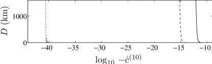
Figure 1: Effective distortion distance $D$ as a function of the isotropic oscillation-free coefficient $-{{\mathaccent 23{c}}}^{(10)}$ in units of GeV^-6 for three neutrino energies: 17 GeV (solid line), 43 GeV (dashed line), and 100 TeV (dotted line).

The energy loss per distance is given by the integral

$${{dE}\over{dx}} = -\int{{d^{3}p^{\prime}}\over{(2\pi)^{3}2E_{p^{\prime}}}}{{d^{3}k}\over{(2\pi)^{3}2E_{k}}}{{d^{3}k^{\prime}}\over{(2\pi)^{3}2E_{k^{\prime}}}}$$ (157)

$$\hskip 10.0pt\times{{(E_{k}+E_{k^{\prime}})(2\pi)^{4}\delta^{4}(p-p^{\prime}-k^{\prime}-k)\sum|{\mathcal{M}}|^{2}}\over{2E_{p}}}$$

$$= -{{C}\over{8}}\int\sin\theta\sin\theta^{\prime}\,d\theta\,d\phi\,d\theta^{\prime}\,d\phi^{\prime}\,d|\vec{\kappa}|$$

$$\hskip 40.0pt\times{{\kappa^{0}\vec{\kappa}^{2}\vec{\kappa}^{\prime 2}}\over{(\kappa^{2}-M_{Z}^{2})^{2}}}{{\partial|\vec{\kappa}^{\prime}|}\over{\partial\kappa^{0}}}{{q\!\cdot\!k\ q^{\prime}\!\cdot\!k^{\prime}}\over{q_{0}E_{k}q_{0}^{\prime}E_{k^{\prime}}}}.$$

The second integral is constrained by the conditions $\kappa=p-p^{\prime}$, $E_{p}\geq\kappa^{0}\geq\sqrt{\vec{\kappa}^{2}+4m^{2}}$, and the constant $C$ is given by $C={2G_{F}^{2}M_{Z}^{4}(1-4s^{2}+8s^{4})}/{(2\pi)^{5}}$. In this second expression we have used the $\delta$-function to perform one integration, introducing the convenient combinations $\kappa^{\mu}=k^{\mu}+k^{\prime\mu}$ and $\kappa^{\prime\mu}=k^{\mu}-k^{\prime\mu}$ with spatial spherical polar angles $(\theta,\phi)$ and $(\theta^{\prime},\phi^{\prime})$.

The integral (157) provides the energy loss per distance in the presence of Dirac-type Lorentz-violating operators of arbitrary mass dimension, including anisotropic effects. To gain some feeling for this integral and to extract estimated bounds on Lorentz violation from Čerenkov spectral distortion, consider the isotropic oscillation-free model with neutrino energy ${{\mathaccent 23{E}}}_{\nu}$ given by Eq. (86) in the preferred frame. For this special case, Eq. (155) shows the factor $q/q_{0}$ becomes $(1,\hat{\boldsymbol{p}})$, so within our assumptions all the Lorentz violation lies in the kinematics. Given values of the coefficients ${{\mathaccent 23{a}}}^{(d)}$, ${{\mathaccent 23{c}}}^{(d)}$ and a specific neutrino energy ${{\mathaccent 23{E}}}_{\nu}$, the integral (157) can be numerically evaluated and used to calculate the effective distortion distance, defined by

$$D(E)\equiv-{{E}\over{dE/dx}}.$$ (158)

For fixed energy, this distance is a rapidly falling function of the coefficients ${{\mathaccent 23{a}}}^{(d)}$ and ${{\mathaccent 23{c}}}^{(d)}$, as illustrated in Fig. 1 for the case $d=10$. It therefore offers a useful measure of the spectral distortion caused by Lorentz violation.

coefficient	17 GeV	43 GeV	100 TeV
$-{{\mathaccent 23{c}}}^{(4)}$	$3\times 10^{-5}$	$6\times 10^{-6}$	$3\times 10^{-11}$
${{\mathaccent 23{a}}}^{(5)}$	$1\times 10^{-6}$	$1\times 10^{-7}$	$4\times 10^{-16}$
$-{{\mathaccent 23{c}}}^{(6)}$	$8\times 10^{-8}$	$3\times 10^{-9}$	$3\times 10^{-21}$
${{\mathaccent 23{a}}}^{(7)}$	$5\times 10^{-9}$	$6\times 10^{-11}$	$2\times 10^{-26}$
$-{{\mathaccent 23{c}}}^{(8)}$	$3\times 10^{-10}$	$1\times 10^{-12}$	$2\times 10^{-31}$
${{\mathaccent 23{a}}}^{(9)}$	$2\times 10^{-11}$	$3\times 10^{-14}$	$2\times 10^{-36}$
$-{{\mathaccent 23{c}}}^{(10)}$	$9\times 10^{-13}$	$8\times 10^{-16}$	$2\times 10^{-41}$

Table 15: Estimated values of isotropic oscillation-free coefficients at which the distortion distance $D(E)$ for Čerenkov pair emission crosses 1000 km for energies 17 GeV, 43 GeV, and 100 TeV. Coefficient units are GeV^4-d.

No substantial spectral distortion is observed at the mean OPERA energy of 17 GeV or ranging up to energies of over 40 GeV opera , and no depletion of atmospheric neutrinos or antineutrinos is detected in IceCube for energies over 100 TeV IceCube11 . Requiring that the distortion distance $D$ at these energies is 1000 km or greater, we can extract conservative limits on isotropic oscillation-free coefficients for Lorentz violation. Table 15 shows estimates for the bounds obtained by taking one coefficient to be nonzero at a time. The bounds are one sided except for the 100 TeV results for ${{\mathaccent 23{a}}}^{(5)}$, ${{\mathaccent 23{a}}}^{(7)}$, and ${{\mathaccent 23{a}}}^{(9)}$, which are on the modulus of the coefficients. The values include ones substantially tighter than the results for the coefficients found in time-of-flight experiments, which are given in Table 13. Note that a complete calculation at 100 TeV is likely to produce sharper limits because at these energies pair emission is expected to be only a small contribution. For example, only about 3% of the on-shell $Z^{0}$ emission generates electron-positron pairs.

An explicit bound on a coefficient for Lorentz violation has recently been obtained from an analysis of the decay rate and energy loss for Čerenkov pair emission cg . This work assumes that Lorentz violation arises only from the isotropic oscillation-free coefficient ${{\mathaccent 23{c}}}^{(4)}$ in the minimal SME, leading to an isotropic constant shift $\delta v=-{{\mathaccent 23{c}}}^{(4)}$ of the muon-neutrino group and phase velocities. The analysis finds the best limit on this type of Lorentz violation comes from IceCube measurements of 100 TeV neutrinos, translating to the one-sided bound ${{\mathaccent 23{c}}}^{(4)}>-8.5\times 10^{-12}$. Also within this particular one-coefficient model, the ICARUS collaboration reports a limit based on the nonobservation of Čerenkov-emission products in the same neutrino beam icarus , which corresponds to the one-sided bound ${{\mathaccent 23{c}}}^{(4)}>-2\times 10^{-8}$. Both these limits are many orders of magnitude tighter than the nonzero negative value of ${{\mathaccent 23{c}}}^{(4)}$ implied by the OPERA result for this one-coefficient model and listed in the first row of Table 13.

VIII Summary

scenario	coefficient	values of $d$	number per $d$
effective	$\big{(}a_{\text{eff}}^{(d)}\big{)}_{jm}^{ab}$	odd, $\geq 3$	$9d^{2}$
	$\big{(}c_{\text{eff}}^{(d)}\big{)}_{jm}^{ab}$	$\begin{cases}d=2&\\ \mbox{even, }\geq 4&\end{cases}$	$\begin{array}[]{c}27\\[-2.0pt] 9d^{2}\end{array}$
	$\big{(}g_{\text{eff}}^{(d)}\big{)}_{jm}^{ab}$	even, $\geq 2$	$12(d^{2}-1)$
	$\big{(}H_{\text{eff}}^{(d)}\big{)}_{jm}^{ab}$	odd, $\geq 3$	$6(d^{2}-1)$
Dirac	$\big{(}a_{L}^{(d)}\big{)}_{jm}^{ab}$	odd, $\geq 3$	$9(d-1)^{2}$
	$\big{(}c_{L}^{(d)}\big{)}_{jm}^{ab}$	even, $\geq 4$	$9(d-1)^{2}$
	$\big{(}m_{l}^{(d)}\big{)}_{jm}^{ab}$	odd, $\geq 5$	$9(d-2)^{2}$
	$\big{(}e_{l}^{(d)}\big{)}_{jm}^{ab}$	even, $\geq 4$	$9(d-2)^{2}$
	$\big{(}g_{l}^{(d)}\big{)}_{jm}^{ab}$	even, $\geq 4$	$9(d-1)^{2}$
	$\big{(}H_{l}^{(d)}\big{)}_{jm}^{ab}$	$\begin{cases}d=3&\\ \mbox{odd, }\geq 5\end{cases}$	$\begin{array}[]{c}27\\[-2.0pt] 9(d-1)^{2}\end{array}$
Majorana	$\big{(}g_{M+}^{(d)}\big{)}_{jm}^{ab}$	even, $\geq 4$	$12d(d-2)$
	$\big{(}H_{M+}^{(d)}\big{)}_{jm}^{ab}$	odd, $\geq 3$	$6d(d-2)$
	$\big{(}a_{l}^{(d)}\big{)}_{jm}^{ab}$	odd, $\geq 3$	$12d(d-2)$
	$\big{(}c_{l}^{(d)}\big{)}_{jm}^{ab}$	even, $\geq 4$	$6d(d-2)$
renormalizable	$\big{(}a_{\text{eff}}^{(3)}\big{)}_{jm}$	3	$81$
	$\big{(}c_{\text{eff}}^{(2)}\big{)}_{jm}$	2	$27$
	$\big{(}c_{\text{eff}}^{(4)}\big{)}_{jm}$	4	$81$
	$\big{(}g_{\text{eff}}^{(2)}\big{)}_{jm}$	2	$36$
	$\big{(}g_{\text{eff}}^{(4)}\big{)}_{jm}$	4	$96$
	$\big{(}H_{\text{eff}}^{(3)}\big{)}_{jm}$	3	$48$
massless	$\big{(}a_{L}^{(d)}\big{)}_{jm}^{ab}$	odd, $\geq 3$	$9(d-1)^{2}$
	$\big{(}c_{L}^{(d)}\big{)}_{jm}^{ab}$	even, $\geq 4$	$9(d-1)^{2}$
	$\big{(}g_{M+}^{(d)}\big{)}_{jm}^{ab}$	even, $\geq 4$	$12d(d-2)$
	$\big{(}H_{M+}^{(d)}\big{)}_{jm}^{ab}$	odd, $\geq 3$	$6d(d-2)$
flavor-blind	$\big{(}a_{\text{fb}}^{(d)}\big{)}_{jm}$	odd, $\geq 3$	$d^{2}$
	$\big{(}c_{\text{fb}}^{(d)}\big{)}_{jm}$	even, $\geq 4$	$(d-1)^{2}$
	$\big{(}g_{\text{fb}}^{(d)}\big{)}_{jm}$	even, $\geq 2$	$2(d^{2}-1)$
oscillation-free	$\big{(}a_{\text{of}}^{(d)}\big{)}_{jm}$	odd, $\geq 3$	$(d-1)^{2}$
	$\big{(}c_{\text{of}}^{(d)}\big{)}_{jm}$	even, $\geq 4$	$(d-1)^{2}$
diagonalizable	$\big{(}a_{\text{d}}^{(d)}\big{)}_{jm}^{a^{\prime}}$	odd, $\geq 3$	$3d^{2}$
	$\big{(}c_{\text{d}}^{(d)}\big{)}_{jm}^{a^{\prime}}$	even, $\geq 4$	$3(d-1)^{2}$
	$\big{(}g_{\text{d}}^{(d)}\big{)}_{jm}^{a^{\prime}}$	even, $\geq 2$	$6(d^{2}-1)$
generic isotropic	${{\mathaccent 23{a}}}^{(d)}_{ab}$	odd, $\geq 3$	9
	${{\mathaccent 23{c}}}^{(d)}_{ab}$	even, $\geq 4$	9
isotropic diag.	${{\mathaccent 23{a}}}^{(d)}_{a^{\prime}}$	odd, $\geq 3$	3
	${{\mathaccent 23{c}}}^{(d)}_{a^{\prime}}$	even, $\geq 4$	3
isotropic osc.-free	${{\mathaccent 23{a}}}^{(d)}$	odd, $\geq 3$	1
	${{\mathaccent 23{c}}}^{(d)}$	even, $\geq 4$	1

Table 16: Summary of spherical coefficients.

In this work, we study the effects of Lorentz and CPT violation on the behavior of fermions, with emphasis on neutrinos. The starting point in Sec. II is the construction of the general quadratic Lagrange density (3) for the propagation and mixing of $N$ species of fermions. This permits Lorentz-violating operators of arbitary mass dimension to be classified and enumerated. A procedure to obtain the leading-order hamiltonian (19) for fermions is described.

In Sec. III, the general theory is specialized to extract the Weyl hamiltonian (32) describing the propagation and mixing of three flavors of left-handed neutrinos in the presence of Lorentz- and CPT-violation involving operators of arbitrary mass dimension. Block diagonalization of the Weyl hamiltonian at leading order in mass and Lorentz violation generates the effective hamiltonian (51) describing dominant modifications to neutrino propagation and mixing. This key result depends on 10 sets of coefficients for Lorentz violation that enter the Lorentz-violating piece (44) of the effective hamiltonian. These 10 sets and some of their features are listed in Table 1. Six involve Dirac-type operators for propagation and mixing, while the other four are Majorana type and describe neutrino-antineutrino mixing.

Since violations of rotation symmetry are a central feature of many searches for Lorentz violation, it is useful to perform a decomposition of the effective hamiltonian and the coefficients using spherical harmonics. The resulting 10 sets of spherical coefficients for Lorentz violation are presented in Sec. IV. Six are of Dirac type and four of Majorana type. This analysis also reveals that the fundamental experimental observables for Lorentz violation in the neutrino sector comprise only four sets of effective spherical coefficients, built from the 10 basic sets according to Eq. (57). The properties of all 14 coefficient sets are given in Table 2.

Various special theoretical scenarios for the spherical coefficients can be countenanced, leading to different experimental predictions. Section V presents several limiting cases of the general formalism. We begin in Sec. V.1 by matching to the renormalizable sector of the SME, revealing some qualitatively new effects that appear at leading order in both mass and Lorentz violation. Some properties of the renormalizable coefficients are given in Table 3.

In Sec. V.2 the limit of massless models is described. This class of models is of interest in part because it offers the potential for an alternative description of neutrino oscillations without invoking mass. The massless coefficients and some properties are given in Table 4.

Another scenario of potential interest, discussed in Sec. V.3, is flavor-blind Lorentz violation. In these models the different neutrino flavors are assumed to experience the same effects, which is a reasonable approximation under some experimental conditions. For example, the limit of oscillation-free propagation is of relevance for certain types of searches for Lorentz violation, such as time-of-flight experiments. Table 5 lists the flavor-blind and oscillation-free coefficients and some of their features.

In Sec. V.4 we consider diagonalizable models, in which all terms in the effective hamiltonian are assumed to be simultaneously diagonalizable. These models offer comparatively simple options for model building with Lorentz violation, while avoiding the complications that appear for general neutrino mixings. The diagonalizable coefficients are tabulated in Table 6.

Finally, various types of isotropic models are studied in Sec. V.5. Isotropy can be enforced only in a preferred inertial frame, with anisotropies appearing in other boosted frames. These models are particularly simple because they cannot have Majorana mixings and their Dirac terms must be isotropic. We discuss generic isotropic models and their restriction to isotropic diagonalizable models and to isotropic oscillation-free models. The coefficients for each case are shown in Table 7.

Table 16 summarizes the various spherical coefficients for Lorentz violation studied in this work. The first column of this table lists the theoretical scenario, the second lists the relevant sets of spherical coefficients, the third provides the range of operator mass dimension $d$ allowed for each coefficient set, and the last column indicates the number of independent coefficients for each value of $d$. The first four rows concern the effective spherical coefficients that are the fundamental observables for any experiment in this framework. The 10 following rows list the 10 basic sets of spherical coefficients arising in the general formalism, which separate into six sets of Dirac type and four sets of Majorana type. The rest of the table concerns the various limiting theoretical scenarios discussed in the text.

In the penultimate sections of the paper, we study experimental implications of the theoretical framework and use existing data on neutrino oscillations and propagation to extract constraints on coefficients for Lorentz and CPT violation. Section VI treats effects on mixing. Two experimentally relevant limits are analyzed. The first is the short-baseline approximation, for which oscillation effects from all sources are small. General expressions for short-baseline oscillation probabilities are given in Eq. (98). These expressions are applied to results from the short-baseline experiments LSND and MiniBooNE to extract maximal attained sensitivities to effects from flavor-mixing Lorentz-violating operators for $d\leq 10$. The results for generic spherical coefficients for Lorentz violation are listed in Table 8, while those for isotropic coefficients are given in Table 9. The second limit is the perturbative approximation, in which the baseline can be arbitrary but the coefficients for Lorentz and CPT violation are assumed small compared to the 3$\nu$SM masses. We derive the mixing probabilities up to second order in Lorentz violation, and we present methods to analyze data from long-baseline experiments. Numerical values of beam-dependent factors relevant to the MINOS, OPERA, and T2K experiments are tabulated in Table 10. As a simple example, we consider the limit of two-flavor mixing and discuss some asymmetries offering sensitivity to CPT violation.

In Sec. VII, we discuss several types of kinematic tests that are independent of mixing. Effects in these tests are controlled by oscillation-free coefficients for Lorentz violation. We consider various time-of-flight measurements, including the OPERA and MINOS experiments, earlier studies at Fermilab, and the supernova SN1987A. These are used to extract constraints on generic oscillation-free coefficients for $d\leq 6$ and on isotropic oscillation-free coefficients for $d\leq 10$. The results are collected in Tables 11, 12, and 13. We also obtain threshold constraints from the observation of high-energy neutrinos by IceCube, presented in Table 14, and we derive the estimated order-of-magnitude bounds from neutrino Čerenkov radiation shown in Table 15.

The analysis in this paper provides a general theoretical framework for the treatment of neutrino propagation and mixing, along with a guide to its application in laboratory experiments and astrophysical observations. We see that searches involving neutrino propagation and mixing offer excellent sensitivities to numerous distinct types of Lorentz and CPT violation. Many coefficients for Lorentz violation remain unconstrained, so a substantial region of untouched territory is open for future exploration using laboratory and astrophysical techniques.

References

• (1) K. Nakamura et al., J. Phys. G 37, 075021 (2010).
• (2) V.A. Kostelecký and S. Samuel, Phys. Rev. D 39, 683 (1989); V.A. Kostelecký and R. Potting, Nucl. Phys. B 359, 545 (1991).
• (3) V.A. Kostelecký and N. Russell, Rev. Mod. Phys. 83, 11 (2011).
• (4) V.A. Kostelecký and R. Potting, Phys. Rev. D 51, 3923 (1995).
• (5) O.W. Greenberg, Phys. Rev. Lett. 89, 231602 (2002); arXiv:1105.0927.
• (6) D. Colladay and V.A. Kostelecký, Phys. Rev. D 55, 6760 (1997); Phys. Rev. D 58, 116002 (1998).
• (7) V.A. Kostelecký, Phys. Rev. D 69, 105009 (2004).
• (8) LSND Collaboration, L.B. Auerbach et al., Phys. Rev. D 72, 076004 (2005).
• (9) M.D. Messier, in CPT and Lorentz Symmetry III, V.A. Kostelecký, ed., World Scientific, Singapore, 2005.
• (10) MINOS Collaboration, P. Adamson et al., Phys. Rev. Lett. 101, 151601 (2008).
• (11) MINOS Collaboration, P. Adamson et al., Phys. Rev. Lett. 105, 151601 (2010).
• (12) IceCube Collaboration, R. Abbasi et al., Phys. Rev. D 82, 112003 (2010).
• (13) MiniBooNE Collaboration, A.A. Aguilar-Arevalo et al., arXiv:1109.3480.
• (14) OPERA Collaboration, T. Adam et al., arXiv:1109.4897.
• (15) V.A. Kostelecký and M. Mewes, Phys. Rev. D 69, 016005 (2004).
• (16) V.A. Kostelecký and M. Mewes, Phys. Rev. D 70, 076002 (2004).
• (17) J.S. Díaz et al., Phys. Rev. D 80, 076007 (2009).
• (18) V.A. Kostelecký and M. Mewes, Phys. Rev. D 70, 031902(R) (2004).
• (19) T. Katori et al., Phys. Rev. D 74, 105009 (2006).
• (20) V. Barger, D. Marfatia, and K. Whisnant, Phys. Lett. B 653, 267 (2007).
• (21) J.S. Díaz and V.A. Kostelecký, Phys. Lett. B 700, 25 (2011); Phys. Rev. D 85, 016013 (2012).
• (22) V. Barger, J. Liao, D. Marfatia, and K. Whisnant, Phys. Rev. D 84, 056014 (2011).
• (23) S. Coleman and S. L. Glashow, Phys. Rev. D 59, 116008 (1999).
• (24) V. Barger, S. Pakvasa, T.J. Weiler, and K. Whisnant, Phys. Rev. Lett. 85, 5055 (2000).
• (25) J.N. Bahcall, V. Barger, and D. Marfatia, Phys. Lett. B 534, 120 (2002).
• (26) A. de Gouvêa, Phys. Rev. D 66, 076005 (2002).
• (27) G. Lambiase, Phys. Lett. B 560, 1 (2003).
• (28) A. Datta, R. Gandhi, P. Mehta, and S.U. Sankar, Phys. Lett. B 597, 356 (2004).
• (29) A. de Gouvêa and C. Peña-Garay, Phys. Rev. D 71, 093002 (2005).
• (30) M.C. Gonzalez-Garcia, F. Halzen and M. Maltoni, Phys. Rev. D 71, 093010 (2005).
• (31) F. Klinkhamer, Phys. Rev. D 71, 113008 (2005).
• (32) Y. Grossman, C. Kilic, J. Thaler, and D.G.E. Walker, Phys. Rev. D 72, 125001 (2005).
• (33) E. Di Grezia, S. Esposito, and G. Salesi, Mod. Phys. Lett. A 21, 349 (2006).
• (34) J.L. Kelley, PoS (QG-PH), 022 (2007).
• (35) N. Cipriano Ribeiro, H. Nunokawa, T. Kajita, S. Nakayama, P. Ko and H. Minakata, Phys. Rev. D 77, 073007 (2008).
• (36) Z. Xiao and B.-Q. Ma, Int. J. Mod. Phys. A 24, 1359 (2009).
• (37) M. Bustamante, A.M. Gago, and C. Peña-Garay, J. Phys. Conf. Ser. 171, 012048 (2009).
• (38) B. Altschul, J. Phys. Conf. Ser. 173 012003 (2009).
• (39) S. Yang and B.-Q. Ma, Int. J. Mod. Phys. A 24, 5861 (2009).
• (40) P. Arias and J. Gamboa, Mod. Phys. Lett. A 25, 277 (2010).
• (41) A. Samanta, Phys. Lett. B 693, 296 (2010).
• (42) A. Bhattacharya, S. Choubey, R. Gandhi, and A. Watanabe, JCAP 1009, 009 (2010).
• (43) C. Liu, J.-t. Tian, and Z.-h. Zhao, Phys. Lett. B 702, 154 (2011).
• (44) C.M. Ho, Phys. Lett. B 702, 398 (2011).
• (45) I. Mocioiu and M. Pospelov, Phys. Lett. B 534, 114 (2002).
• (46) R. Brustein, D. Eichler, and S. Foffa, Phys. Rev. D 65, 105006 (2002).
• (47) G. Lambiase, Phys. Rev. D 71, 065005 (2005).
• (48) D. Hooper, D. Morgan, and E. Winstanley, Phys. Rev. D 72, 065009 (2005).
• (49) A.E. Bernardini and O. Bertolami, Phys. Rev. D 77, 085032 (2008).
• (50) S. Ando, M. Kamionkowski, and I. Mocioiu, Phys. Rev. D 80, 123522 (2009).
• (51) B. Altschul, Phys. Rev. D 84, 091902 (2011).
• (52) N. Qin and B.-Q. Ma, arXiv:1110.4443.
• (53) S. Choubey and S.F. King, Phys. Lett. B 586, 353 (2004).
• (54) S. Hollenberg, O. Micu, and H. Päs, Phys. Rev. D 80, 053010 (2009).
• (55) S. Hollenberg, O. Micu, and P.B. Pal, arXiv:1112.1523.
• (56) V.A. Kostelecký and N. Russell, Phys. Lett. B 693, 443 (2010); V.A. Kostelecký, Phys. Lett. B 701, 137 (2011).
• (57) V.A. Kostelecký and R. Lehnert, Phys. Rev. D 63, 065008 (2001).
• (58) M.S. Berger and V.A. Kostelecký, Phys. Rev. D 65, 091701 (2002); P.A. Bolokhov, S.G. Nibbelink, and M. Pospelov, Phys. Rev. D 72, 015013 (2005).
• (59) M. Hayakawa, Phys. Lett. B 478, 394 (2000).
• (60) The leading-order action is presented in S.M. Carroll et al., Phys. Rev. Lett. 87, 141601 (2001).
• (61) V.A. Kostelecký and M. Mewes, Ap. J. Lett. 689, L1 (2008); Phys. Rev. D 80, 015020 (2009).
• (62) J. Alfaro, H.A. Morales-Técotl, and L.F. Urrutia, Phys. Rev. Lett. 84, 2318 (2000).
• (63) T. Jacobson, S. Liberati, and D. Mattingly, Phys. Rev. D 67, 124011 (2003).
• (64) J. Christian, Phys. Rev. D 71, 024012 (2005).
• (65) U. Jacob and T. Piran, Nature Phys. 3, 87 (2007).
• (66) P.A. Bolokhov and M. Pospelov, Phys. Rev. D 77, 025022 (2008).
• (67) A. Sakharov, J. Ellis, N. Harries, A. Meregaglia, and A. Rubbia, J. Phys. Conf. Ser. 171, 012039 (2009).
• (68) D.M. Mattingly, L. Maccione, M. Galaverni, S. Liberati, and G. Sigl, JCAP 1002, 007 (2010).
• (69) A. Chodos et al., Phys. Lett. B 150, 431 (1985).
• (70) A. Chodos et al., Mod. Phys. Lett. A 7, 467 (1992).
• (71) V.A. Kostelecký, in F. Mansouri and J.J. Scanio, eds., Topics on Quantum Gravity and Beyond, World Scientific, Singapore, 1993.
• (72) A. Chodos and V.A. Kostelecký, Phys. Lett. B 336, 295 (1994).
• (73) J. Rembieliński, Int. J. Mod. Phys. A 12, 1677 (1997).
• (74) R. Ehrlich, Phys. Rev. D 60, 017302 (1999).
• (75) M.J. Radzikowski, arXiv:1007.5418.
• (76) G.F. Giudice, S. Sibiryakov, and A. Strumia, arXiv:1109.5682.
• (77) A. Drago, I. Masina, G. Pagliara, and R. Tripiccione, arXiv:1109.5917.
• (78) J. Alexandre, J. Ellis, and N.E. Mavromatos, arXiv:1109.6296.
• (79) A.G. Cohen and S.L. Glashow, Phys. Rev. Lett. 107, 181803 (2011).
• (80) L. Gonzalez-Mestres, arXiv:1109.6630.
• (81) X.-J. Bi, P.-F. Yin, Z.-H. Yu, and Q. Yuan, Phys. Rev. Lett. 107, 241802 (2011).
• (82) R. Cowsik, S. Nussinov, and U. Sarkar, Phys. Rev. Lett. 107, 251801 (2011).
• (83) N.D. Hari Dass, arXiv:1110.0351.
• (84) J.M. Carmona and J.L. Cortés, arXiv:1110.0430.
• (85) G. Amelino-Camelia, L. Friedel, J. Kowalski-Glikman, and L. Smolin, arXiv:1110.0521.
• (86) L. Maccione, S. Liberati, and D.M. Mattingly, arXiv:1110.0783.
• (87) S.-S. Xue, Phys. Lett. B 706, 213 (2011).
• (88) R.A. Konoplya and A. Zhidenko, arXiv:1110.2015.
• (89) F.R. Klinkhamer, arXiv:1110.2146.
• (90) U.D. Jentschura and B.J. Wundt, arXiv:1110.4171.
• (91) C.A.G. Almeida, M.A. Anacleto, F.A. Brito, and E. Passos, arXiv:1111.0093.
• (92) S. Mohanty and S. Rao, arXiv:1111.2725.
• (93) M. Li, D. Liu, J. Meng, T. Wang, and L. Zhou, arXiv:1111.3294.
• (94) R. Horvat, A. Ilakovac, P. Schupp, J. Trampetić, and J. You, arXiv:1111.5941.
• (95) M. Schreck, arXiv:1111.7268.
• (96) M. Mannarelli, M. Mitra, F.L. Villante, and F. Vissani, arXiv:1112.0169.
• (97) Y. Huo, T. Li, Y. Liao, D.V. Nanopoulos, and Y. Qi, arXiv:1112.0264.
• (98) F. Bezrukov and H.M. Lee, arXiv:1112.1299.
• (99) S. Mohanty and S. Rao, arXiv:1112.2981.
• (100) V.A. Kostelecký and M. Mewes, in preparation.
• (101) Y. Nambu, Phys. Rev. Lett. 4, 380 (1960); J. Goldstone, Nuov. Cim. 19, 154 (1961); J. Goldstone, A. Salam, and S. Weinberg, Phys. Rev. 127, 965 (1962).
• (102) V.A. Kostelecký and S. Samuel, Phys. Rev. D 40, 1886 (1989); Phys. Rev. Lett. 63, 224 (1989); R. Bluhm and V.A. Kostelecký, Phys. Rev. D 71, 065008 (2005); R. Bluhm et al., Phys. Rev. D 77, 065020 (2008); O. Bertolami and J. Páramos, Phys. Rev. D 72, 044001 (2005); Q.G. Bailey and V.A. Kostelecký, Phys. Rev. D 74, 045001 (2006); M.D. Seifert, Phys. Rev. D 79, 124012 (2009); Phys. Rev. D 81, 065010 (2010); J. Alfaro and L.F. Urrutia, Phys. Rev. D 81, 025007 (2010).
• (103) V.A. Kostelecký and R. Potting, Gen. Rel. Grav. 37, 1675 (2005); Phys. Rev. D 79, 065018 (2009); S.M. Carroll, H. Tam, and I.K. Wehus, Phys. Rev. D 80, 025020 (2009); J.L. Chkareuli, C.D. Froggatt, and H.B. Nielsen, Nucl. Phys. B 848, 498 (2011).
• (104) N. Arkani-Hamed, H.-C. Cheng, M. Luty, and J. Thaler, JHEP 0507, 029 (2005); V.A. Kostelecký and J.D. Tasson, Phys. Rev. Lett. 102, 010402 (2009); Phys. Rev. D 83, 016013 (2011); B. Altschul et al., Phys. Rev. D 81, 065028 (2010).
• (105) V.A. Kostelecký, N. Russell, and J. Tasson, Phys. Rev. Lett. 100, 111102 (2008); B.R. Heckel, E.G. Adelberger, C.E. Cramer, T.S. Cook, S. Schlamminger and U. Schmidt, Phys. Rev.  D 78, 092006 (2008).
• (106) Y. Bonder and D. Sudarsky, Rep. Math. Phys. 64, 169 (2009).
• (107) M. Gell-Mann, P. Ramond, and R. Slansky, in P. van Nieuwenhuizen and D.Z. Freedman, ed., Supergravity, North Holland, Amsterdam, 1979; T. Yanagida, Prog. Theor. Phys. 64, 1103 (1980); R. Mohapatra and G. Senjanović, Phys. Rev. Lett. 44, 912 (1980); J. Schechter and J.W.F. Valle, Phys. Rev. D 22, 2227 (1980).
• (108) V.A. Kostelecký, C.D. Lane, and A.G.M. Pickering, Phys. Rev. D 65, 056006 (2002); V.A. Kostelecký and A.G.M. Pickering, Phys. Rev. Lett. 91, 031801 (2003); B. Altschul and V.A. Kostelecký, Phys. Lett. B 628, 106 (2005); G. de Berredo-Peixoto and I.L. Shapiro, Phys. Lett. B 642, 153 (2006); D. Colladay and P. McDonald, Phys. Rev. D 75, 105002 (2007); Phys. Rev. D 77, 085006 (2008); Phys. Rev. D 79, 125019 (2009); P. Arias, H. Falomir, J. Gamboa, F. Méndez, and F.A. Schaposnik, Phys. Rev. D 76, 025019 (2007); D. Anselmi, Ann. Phys. 324, 874 (2009); Ann. Phys. 324, 1058 (2009); A. Ferrero and B. Altschul, Phys. Rev. D 84, 065030 (2011).
• (109) KamLAND Collaboration, T. Araki et al., Phys. Rev. Lett. 94, 081801 (2005); S. Abe et al., Phys. Rev. Lett. 100, 221803 (2008).
• (110) Borexino Collaboration, G. Bellini et al., Phys. Rev. D 82, 033006 (2010).
• (111) R. Bluhm et al., Phys. Rev. D 68, 125008 (2003); Phys. Rev. Lett. 88, 090801 (2002).
• (112) V.A. Kostelecký and M. Mewes, Phys. Rev. D 66, 056005 (2002).
• (113) MiniBooNE Collaboration, A.A. Aguilar-Arevalo et al., Phys. Rev. Lett. 98, 231801 (2007); Phys. Rev. Lett. 102, 101802 (2009).
• (114) MiniBooNE Collaboration, A.A. Aguilar-Arevalo et al., Phys. Rev. Lett. 105, 181801 (2010).
• (115) LSND Collaboration, A. Aguilar et al., Phys. Rev. D 64, 112007 (2001).
• (116) MINOS Collaboration, P. Adamson et al., Phys. Rev. Lett. 107, 021801 (2011).
• (117) J. Lukierski and A. Nowicki, Acta Phys. Pol. B 33, 2537 (2002); S. Judes and M. Visser, Phys. Rev. D 68, 045001 (2003); N. Jafari and A. Shariati, AIP Conf. Proc. 841, 462 (2006).
• (118) J. Alonso et al., arXiv:1006.0260.
• (119) Double Chooz Collaboration, F. Ardellier et al., hep-ex/0606025.
• (120) Daya Bay Collaboration, X. Guo et al., hep-ex/0701029.
• (121) RENO Collaboration, J.K. Ahn et al., arXiv:1003.1391.
• (122) Super-Kamiokande Collaboration, S. Fukuda et al., Nucl. Instrum. Meth. A 501, 418 (2003).
• (123) V.A. Kostelecký, Phys. Rev. Lett. 80, 1818 (1998).
• (124) KLOE Collaboration, A. Di Domenico, J. Phys. Conf. Ser. 171, 012008 (2009); BaBar Collaboration, B. Aubert et al., Phys. Rev. Lett. 100, 131802 (2008); FOCUS Collaboration, J.M. Link et al., Phys. Lett. B 556, 7 (2003); KTeV Collaboration, H. Nguyen, hep-ex/0112046; V.A. Kostelecký and R.J. Van Kooten, Phys. Rev. D 82, 101702(R) (2010); V.A. Kostelecký, Phys. Rev. D 64, 076001 (2001); Phys. Rev. D 61, 016002 (1999).
• (125) MINOS Collaboration, P. Adamson et al., Phys. Rev. D 76, 072005 (2007).
• (126) G.R. Kalbfleisch, N. Baggett, E.C. Fowler, and J. Alspector, Phys. Rev. Lett. 43, 1361 (1979); J. Alspector et al., Phys. Rev. Lett. 36, 837 (1976).
• (127) K. Hirata et al., Phys. Rev. Lett. 58, 1490 (1987); R.M. Bionta et al., Phys. Rev. Lett. 58, 1494 (1987); M.J. Longo, Phys. Rev. D 36, 3276 (1987).
• (128) T2K Collaboration, Y. Itow et al., hep-ex/0106019.
• (129) Borexino Collaboration, G. Alimonti et al., arXiv:0806.2400.
• (130) ICARUS Collaboration, S. Amerio et al., Nucl. Instrum. Meth. A 527, 329 (2004).
• (131) A recent discussion and review of threshold effects for general processes is V. Baccetti, K. Tate, and M. Visser, arXiv:1111.6340.
• (132) IceCube Collaboration, R. Abbasi et al., Phys. Rev. D 84, 072001 (2011).
• (133) S.J. Brodsky and S. Gardner, arXiv:1112.1090.
• (134) D. Colladay and V.A. Kostelecký, Phys. Lett. B 511, 209 (2001).
• (135) ICARUS Collaboration, M. Antonello et al., arXiv:1110.3763.