Generation of a two-photon state from a quantum dot in a microcavity under incoherent and coherent continuous excitation

Abstract

We analyze the impact of both an incoherent and a coherent continuous excitation in our proposal to generate a two-photon state from a quantum dot in a microcavity [New J. Phys. 13, 113014 (2011)]. A comparison between exact numerical results and analytical formulas provides the conditions to efficiently generate indistinguishable and simultaneous pairs of photons under both types of excitation.

1 INTRODUCTION

A single quantum dot in a cavity can be turned into a two-photon emitter by tuning the cavity frequency into resonance with half the biexciton energy [1]. Since the biexciton frequency can be far from twice the exciton energy—thanks to the binding energy—the exciton states can be very far from the cavity too. This allows their emission through the cavity to be suppressed while Purcell-enhancing the two-photon emission from the biexciton [2]. The principle has been recently realised in a system well into the strong coupling regime [3], where the authors have observed a strong enhancement of the photoluminescence spectrum at the two-photon resonance (2PR), compatible with very low number of photons. This means that the emission was in the spontaneous (or linear) regime. In this experiment, the system was excited via a continuous excitation of the wetting layer, resulting in an incoherent population of the dot levels.

Incoherent excitation is a convenient way of probing the system, typically used to characterised the level structure and optical resonances. However, it may have a substantial and undesired impact on the quantum properties, namely, an increase of decoherence and dephasing in the dynamics (even more so when the features of interest require a pumping to high rungs of excitation, as it is the case for the Jaynes-Cummings nonlinearities [4], one atom laser [5, 6, 7] or entangled photon pair generation [8], among others). In general, it is advisable to include incoherent excitation when describing experimental results in order to interpret them correctly (e. g. strong coupling [9, 6, 10], superradiance [11, 12], phase transitions [13], etc.)

Coherent excitation, close to resonance to the quantum dot levels, provides a second possibility to probe the system. To this intent, one can for instance apply a laser whose polarization is orthogonal to that of the cavity mode, in order not to excite cavity photons (directly or indirectly though the state with the cavity polarization). Coherent excitation may seem like a better choice because it does not introduce extra decoherence in the dynamics. Moreover, if the laser is also tuned to the two-photon resonance, it will excite the biexciton directly with high probability [14]. However, one must remain in the linear regime as well in order not to dress the system [15], adding excitation-induced features.

In this work, we study theoretically the two-photon emission under a low continuous excitation of both types. In Section 2, we obtain numerically the dot-cavity steady state and locate the one- and two-photon resonances in the system. In Section 3, we develop an analytical approach at the two-photon resonance, consisting in solving the effective dot dynamics and deriving the cavity properties from physical arguments. The comparison between the numerical and analytical results provides the limiting excitation before the two-photon emission is hindered by decoherence or dressed states. The formulas provide optimum pumping strength and information on the differences between the two types of excitation.

2 TWO-PHOTON RESONANCE UNDER CONTINUOUS EXCITATION

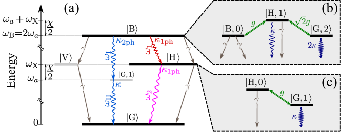
Figure 1: Level scheme of a quantum dot coupled to a cavity mode with linear polarization H at the 2PR. In (a), the quantum dot four-level system is shown including all loss channels: on the one hand, the excitonic spontaneous decay, $\gamma$, and the one-cavity-photon decay, $\kappa_{\mathrm{1P}}$, taking place at frequencies $\omega_{1}$ and $\omega_{2}$; on the other hand, the two-cavity-photon Purcell enhanced decay, $\kappa_{\mathrm{2P}}$, at the cavity frequency $\omega_{\mathrm{I,II}}\approx\omega_{a}$. In (b) is shown how (thanks to the dispersive coupling to the cavity) the state $\left|\mathrm{B}\right\rangle\approx\left|\mathrm{B,0}\right\rangle$ acquires a small component from other states with one and two photons, giving rise to the effective one- and two-photon decay rates $\kappa_{\mathrm{1P}}$ and $\kappa_{\mathrm{2P}}$. In (c), id. but for the state $\left|\mathrm{H}\right\rangle\approx\left|\mathrm{H,0}\right\rangle$ that acquires a small one-photon component that leads to $\kappa_{\mathrm{1P}}$.

The system consists of a dot embedded in a microcavity, coupled only to one of its modes, polarised along a direction that we call horizontal (H). It is, therefore, convenient to study the dot in the basis of the two orthogonal linear polarizations H and V: $\{\left|\mathrm{G}\right\rangle,\left|\mathrm{V}\right\rangle,\left|\mathrm{H}\right\rangle,\left|\mathrm{B}\right\rangle\}$, where G stands for the ground state, V for vertically polarised dot state and B for the biexciton state, that is, having both spin-up and spin-down states (or H and V polarised states) excited. The total Hilbert space including the cavity degree of freedom is expanded in terms of the basis $\{\left|\mathrm{G}n\right\rangle,\left|\mathrm{V}n\right\rangle,\left|\mathrm{H}n\right\rangle,\left|\mathrm{B}n\right\rangle\}$ with $n=0,\ldots,\infty$ is the number of photons. The Hamiltonian of the system reads ($\hbar=1$):

$$H_{\mathrm{dot-cav}}=\underbrace{\omega_{\mathrm{X}}\big{(}\left|\mathrm{V}\right\rangle\left\langle\mathrm{V}\right|+\left|\mathrm{H}\right\rangle\left\langle\mathrm{H}\right|\big{)}+(2\omega_{\mathrm{X}}-\chi)\left|\mathrm{B}\right\rangle\left\langle\mathrm{B}\right|}_{\text{$H_{\mathrm{dot}}$}}+\underbrace{\omega_{a}a^{\dagger}a}_{\text{$H_{\mathrm{cavity}}$}}+\underbrace{g\sum_{i=\mathrm{H,V}}\big{[}a^{\dagger}(\left|\mathrm{G}\right\rangle\left\langle i\right|+\left|i\right\rangle\left\langle\mathrm{B}\right|)+\text{h. c.}\big{]}}_{\text{$H_{\mathrm{coupling}}$}}\,,$$ (1)

where $a$ is the cavity field annihilation operator (boson) with frequency $\omega_{a}$. We consider the excitonic states at the same frequency $\omega_{\mathrm{X}}$ since a possible splitting between them does not affect our results. The binding energy of the biexciton state, $\chi$, is the key parameter to turn the system into a two-photon emitter. If the cavity is tuned so that two photons match the biexciton frequency, $\omega_{a}=\omega_{\mathrm{X}}-\chi/2$, as in Fig. 1(a), the paired emission of cavity photons is enhanced by two-photon Purcell effect [1, 2].

Dissipation and excitation are included in the master equation

$$\partial_{t}\tilde{\rho}=i[\tilde{\rho},H_{\mathrm{dot-cav}}]+\mathbf{\tilde{L}}_{\mathrm{decay}}(\tilde{\rho})+\mathbf{L}_{\mathrm{coh}}(\tilde{\rho})+\mathbf{L}_{\mathrm{incoh}}(\tilde{\rho})\,,$$ (2)

in the following form:

$$\mathbf{\tilde{L}}_{\mathrm{decay}}(\tilde{\rho})=\frac{\kappa}{2}\mathcal{L}_{a}(\tilde{\rho})+\frac{\gamma}{2}\sum_{i=\mathrm{V,H}}\Big{[}\mathcal{L}_{\left|\mathrm{G}\right\rangle\left\langle i\right|}+\mathcal{L}_{\left|i\right\rangle\left\langle\mathrm{B}\right|}\Big{]}(\tilde{\rho})\,,$$ (3a)

$$\mathbf{L}_{\mathrm{coh}}(\tilde{\rho})=i\Omega_{\mathrm{V}}[\tilde{\rho},\left|\mathrm{G}\right\rangle\left\langle\mathrm{V}\right|+\left|\mathrm{V}\right\rangle\left\langle\mathrm{B}\right|+\text{h. c.}]\,,$$ (3b)

$$\mathbf{L}_{\mathrm{incoh}}(\tilde{\rho})=\frac{P}{2}\sum_{i=\mathrm{V,H}}\Big{[}\mathcal{L}_{\left|\mathrm{i}\right\rangle\left\langle\mathrm{G}\right|}+\mathcal{L}_{\left|\mathrm{B}\right\rangle\left\langle\mathrm{i}\right|}\Big{]}(\tilde{\rho})\,.$$ (3c)

where $\mathcal{L}_{c}(\rho)=2c\rho c^{\dagger}-c^{\dagger}c\rho-\rho c^{\dagger}c$ is in the Lindblad form. We call $\kappa$ the cavity losses and $\gamma$ the exciton relaxation rates. The variable $\tilde{\rho}$ refers to the total cavity-dot density matrix while $\rho$ refers to the reduced dot density matrix, tracing out the cavity degree of freedom. We consider the separate action of two types of continuous excitation: coherent excitation (resonant driving of the dot) with vertical polarization, $\mathbf{L}_{\mathrm{coh}}$, and incoherent excitation (off-resonant driving of the wetting layer) affecting all four levels, $\mathbf{L}_{\mathrm{incoh}}$. In the case of coherent excitation, the master equation is in a frame rotating at the laser frequency and, therefore, all frequencies are referred to the laser one $\omega_{L}$, which we set at the two-photon resonance to maximise the biexciton population: $\omega_{L}=\omega_{\mathrm{X}}-\chi/2$.

We solve equation Eq. (2) in the steady state by setting $\partial_{t}\tilde{\rho}=0$. First, this is done numerically with a sufficient truncation in the number of photons. We take the exciton relaxation rate, $\gamma$, as the smallest parameter in the system and the biexciton binding energy, $\chi$, as the largest, which is the typical experimental situation [3]. In order to increase efficiency of the two photon emission, the system is in the regime of strong coupling, that is, we assume parameters in the range [2] $\gamma\ll\kappa\lessapprox g\ll\chi$.

The main quantities of interest—characterising the cavity emission—are the steady state mean cavity photon number $n_{a}=\langle a^{\dagger}a\rangle$ and the $Q$ Mandel factor, $Q=n_{a}(G^{(2)}/n_{a}^{2}-1)$, related to the second order coherence function at zero delay, $G^{(2)}=\langle a^{\dagger}a^{\dagger}aa\rangle$. The $Q$ factor quantifies bunching ($Q>0$) and antibunching ($Q<0$) in the emission, taking into account the available signal $n_{a}$. We plot $Q$ and $n_{a}$ in Fig. 2 under weak incoherent (a) and coherent (b) excitation.

As a first step, we tune the cavity frequency through the system, probing the different resonances. Keeping in mind the level structure of Fig. 1, we locate the two-photon resonance (2PR) by a clear bunching peak of the $Q$-factor at $\omega_{a}\approx\omega_{\mathrm{B}}/2=\omega_{\mathrm{X}}-\chi/2$ (at $-10g$ in the figures). This corresponds to the simultaneous emission of two cavity photons from $\left|\mathrm{B}\right\rangle$ as shown in Refs. [1, 2]. On the other hand, at the two possible one-photon resonances (1PR), namely at $\omega_{a}=\omega_{1}\approx\omega_{\mathrm{X}}-\chi$ and $\omega_{a}=\omega_{2}\approx\omega_{\mathrm{X}}$ (at $-20g$ and $0$ in the figures), the $Q$-factor drops or even becomes negative. These features, accompanied by an enhancement in the cavity emission $n_{a}$, especially at the 2PR, are in agreement with the properties found for an ideal device that can be prepared in the biexciton state $\left|\mathrm{B}0\right\rangle$ [2]. There are, however, some differences between this ideal case and the two types of excitation. For instance, under coherence excitation, two new two-photon resonances appear at $\omega_{\mathrm{X}}-3\chi/4$ and $\omega_{\mathrm{X}}-\chi/4$ (at $-15g$ and $-5g$ in the figure) that we call $(i)$ and $(ii)$. They arise when two photons match the transitions to Raman virtual states created by the laser, close to $\left|\mathrm{G}\right\rangle$ and $\left|\mathrm{B}\right\rangle$, respectively, as depicted on the right hand side of Fig. 2. These are excitation induced resonances. They show how the cavity emission can be strongly and qualitatively affected by the laser even though it has the orthogonal polarization.

In order to analyse other more subtle issues related to the excitation, regarding efficiency, degree of simultaneity or indistinguishability of the two-photon emission at the 2PR, we will carry out some approximations on Eq. (2) and obtain analytical expressions for the dot populations, $n_{a}$ and $Q$ .

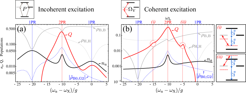
Figure 2: Steady state of the system under (a) incoherent and (b) coherent excitation when sweeping the cavity frequency through the different resonances. The results are exact, obtained by solving numerically the corresponding full master equation (2). We plot $Q$, $n_{a}$, $\rho_{\mathrm{B,B}}$, $\rho_{\mathrm{H,H}}$ and $|\tilde{\rho}_{\mathrm{B0,G2}}|$. With vertical guide lines we have marked the two-photon and one-photon resonances. The laser frequency in (b) is set at the two-photon resonant excitation, $\omega_{\mathrm{L}}=\omega_{\mathrm{X}}-\chi/2$. In this case, we also find two additional bunching peaks in $Q$, (i) and (ii), due to the two-cavity-photon resonance with virtual (Raman) states driven by the laser. Parameters: $\chi=20g$, $\kappa=g$, $\gamma=0.01g$, $P=0.06g$, $\Omega_{\mathrm{V}}=0.5g$.

3 ANALYTICAL RESULTS

Let us tune the cavity to the two-photon resonance (2PR), $\omega_{a}\approx\omega_{\mathrm{X}}-\chi/2$, as in Fig. 1. Here, the effective one-photon and two-photon coupling strengths are much smaller than the cavity decay rate, $g_{\mathrm{1P}}\approx g\kappa/\chi$ and $g_{\mathrm{2P}}\approx 4g^{2}/(\sqrt{2}\chi)\ll\kappa$ [1]. Therefore, we can adiabatically eliminate the cavity and consider only the quantum dot effective dynamics in its reduced Hilbert space. The cavity simply provides three extra decay channels that are Purcell suppressed/enhanced, given by the rates [2]:

$$\kappa_{\mathrm{1P}}=4g_{\mathrm{1P}}^{2}/\kappa\quad\text{and}\quad\kappa_{\mathrm{2P}}=4g_{\mathrm{2P}}^{2}/(2\kappa)\,.$$ (4)

The first one provides a second de-excitation channel from $\left|\mathrm{B}\right\rangle$ to $\left|\mathrm{H}\right\rangle$ and from $\left|\mathrm{H}\right\rangle$ to $\left|\mathrm{G}\right\rangle$ via the emission of one cavity photon. The second rate provides a third de-excitation channel from $\left|\mathrm{B}\right\rangle$ to $\left|\mathrm{G}\right\rangle$ via the emission of two cavity photons.

3.1 Quantum dot properties

The master equation for the reduced dot density matrix $\rho$, where the cavity degree of freedom has been traced out, reads:

$$\partial_{t}\rho= i[\rho,H_{\mathrm{dot}}]+\mathbf{L}_{\mathrm{decay}}(\rho)+\mathbf{L}_{\mathrm{coh}}(\rho)+\mathbf{L}_{\mathrm{incoh}}(\rho)\,,$$ (5a)

$$\mathbf{L}_{\mathrm{decay}}(\rho)= \frac{\gamma+\kappa_{1P}}{2}\Big{[}\mathcal{L}_{\left|\mathrm{G}\right\rangle\left\langle H\right|}+\mathcal{L}_{\left|H\right\rangle\left\langle\mathrm{B}\right|}\Big{]}(\rho)+\frac{\kappa_{2P}}{2}\mathcal{L}_{\left|\mathrm{G}\right\rangle\left\langle B\right|}(\rho)+\frac{\gamma}{2}\Big{[}\mathcal{L}_{\left|\mathrm{G}\right\rangle\left\langle V\right|}+\mathcal{L}_{\left|V\right\rangle\left\langle\mathrm{B}\right|}\Big{]}(\rho)\,.$$ (5b)

For simplicity, we neglect the small Stark shifts induced by the dispersive coupling on the exciton and cavity frequencies, of the order of $g_{\mathrm{1P}}$, $g_{\mathrm{2P}}$.

The equations under incoherent excitation involve only the populations:

$$\partial_{t}\rho_{\mathrm{G,G}}=-2P\rho_{\mathrm{G,G}}+\gamma\rho_{\mathrm{V,V}}+(\gamma+\kappa_{\mathrm{1P}})\rho_{\mathrm{H,H}}+\kappa_{\mathrm{2P}}\rho_{\mathrm{B,B}}\,,$$ (6a)

$$\partial_{t}\rho_{\mathrm{V,V}}=P\rho_{\mathrm{G,G}}-(\gamma+P)\rho_{\mathrm{V,V}}+\gamma\rho_{\mathrm{B,B}}\,,$$ (6b)

$$\partial_{t}\rho_{\mathrm{H,H}}=P\rho_{\mathrm{G,G}}-(\gamma+P+\kappa_{\mathrm{1P}})\rho_{\mathrm{H,H}}+(\gamma+\kappa_{\mathrm{1P}})\rho_{\mathrm{B,B}}\,,$$ (6c)

$$\partial_{t}\rho_{\mathrm{B,B}}=P\rho_{\mathrm{V,V}}+P\rho_{\mathrm{H,H}}-(2\gamma+\kappa_{\mathrm{1P}}+\kappa_{\mathrm{2P}})\rho_{\mathrm{B,B}}\,.$$ (6d)

Together with the normalization Tr$(\rho)=1$, they provide analytical expressions, such as:

$$\rho_{\mathrm{H,H}}\approx\frac{P\gamma\Gamma_{\mathrm{B}}+P^{2}(\Gamma_{\mathrm{B}}+\Gamma_{\mathrm{H}}-\gamma)}{\gamma\Gamma_{\mathrm{B}}\Gamma_{\mathrm{H}}+2P\big{[}\gamma(\Gamma_{\mathrm{B}}-\Gamma_{\mathrm{H}})+\Gamma_{\mathrm{B}}\Gamma_{\mathrm{H}}\big{]}+3P^{2}\Gamma_{\mathrm{B}}+2P^{3}}\xrightarrow{P\rightarrow 0}\frac{1}{\Gamma_{\mathrm{H}}}P\,,$$ (7a)

$$\rho_{\mathrm{B,B}}\approx\frac{P^{2}(\Gamma_{\mathrm{H}}+\gamma)+2P^{3}}{\gamma\Gamma_{\mathrm{B}}\Gamma_{\mathrm{H}}+2P\big{[}\gamma(\Gamma_{\mathrm{B}}-\Gamma_{\mathrm{H}})+\Gamma_{\mathrm{B}}\Gamma_{\mathrm{H}}\big{]}+3P^{2}\Gamma_{\mathrm{B}}+2P^{3}}\xrightarrow{P\rightarrow 0}\frac{\Gamma_{\mathrm{H}}+\gamma}{\gamma\Gamma_{\mathrm{B}}\Gamma_{\mathrm{H}}}P^{2}\,,$$ (7b)

where $\Gamma_{\mathrm{B}}=2\gamma+\kappa_{\mathrm{1P}}+\kappa_{\mathrm{2P}}$ and $\Gamma_{\mathrm{H}}=\gamma+\kappa_{\mathrm{1P}}$ are the dissipation rates of levels the B and H. At vanishing pumping, we find the expected linear increase for single exciton populations and square increase for the biexciton population. In Fig. 3(a) we give an example of the quality of the approximation. Both the numerical exact solution of the full master equation (solid lines) and the approximated formulas (7) (dashed lines) are plotted for increasing excitation. They match almost perfectly for the whole pumping range. Eventually the system saturates on the biexciton state (not shown).

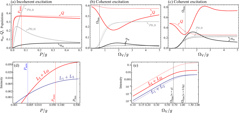
Figure 3:
First row: Steady state of the system at the 2PR under (a) incoherent and (b), (c) coherent excitation as a function of the corresponding excitation rates. The quantities $Q$, $n_{a}$, $\rho_{\mathrm{B,B}}$ and $\rho_{\mathrm{H,H}}$ are shown. The exact numerical results appear with solid lines and the analytical approximations discussed in the text in dashed lines. The formulas for $n_{a}$ and $Q$ are a good approximation for $P<P_{\mathrm{lim}}$ and $\Omega_{\mathrm{V}}<\Omega_{\mathrm{lim}}$. The maximum $Q$ under incoherent excitation is achieved at $P_{\mathrm{max}}=0.066g$, which is the parameter used in Fig. 2(a). The optimum $Q$ under coherent excitation is achieved at vanishing pumping. Parameters: $\chi=20g$, $\omega_{a}=\omega_{\mathrm{X}}-\chi/2$. In (a), (b) $\kappa=g$, giving $\kappa_{\mathrm{1P}}=0.01g$, $\kappa_{\mathrm{2P}}=0.04g$, $P_{\mathrm{lim}}=0.5g$ and $\Omega_{\mathrm{lim}}=0.63g$. In (c) $\kappa=0.3g$ giving $\kappa_{\mathrm{1P}}=0.003g$, $\kappa_{\mathrm{2P}}=0.13g$ and $\Omega_{\mathrm{lim}}=1.15g$. In (a), $\gamma=0.01g$. In (b), (c), $\gamma=0.1g$.
Second row: Analytical approximations for the two contributions to the cavity emission: from single photons, $L_{1}+L_{2}$, and from pairs of photons, $L_{\mathrm{I}}+L_{\mathrm{II}}$. Panel (d) corresponds to situation (a) and panel (e) to situations (b) and (c), plotted in solid and dashed lines, respectively.

The equations under coherent excitation involve not only the populations but also some off-diagonal terms of the density matrix:

$$\partial_{t}\rho_{\mathrm{G,G}}=\gamma\rho_{\mathrm{V,V}}+\Gamma_{\mathrm{H}}\rho_{\mathrm{H,H}}+\kappa_{\mathrm{2P}}\rho_{\mathrm{B,B}}-i\Omega_{\mathrm{V}}(\rho_{\mathrm{V,G}}-\rho_{\mathrm{G,V}})\,,$$ (8a)

$$\partial_{t}\rho_{\mathrm{G,V}}=\big{(}i\frac{\chi}{2}-\frac{\gamma}{2}\big{)}\rho_{\mathrm{G,V}}+i\Omega_{\mathrm{V}}(\rho_{\mathrm{G,G}}-\rho_{\mathrm{V,V}}+\rho_{\mathrm{G,B}})\,,$$ (8b)

$$\partial_{t}\rho_{\mathrm{G,B}}=-\big{(}\frac{\gamma+\Gamma_{\mathrm{H}}+\kappa_{\mathrm{2P}}}{2}\big{)}\rho_{\mathrm{G,B}}-i\Omega_{\mathrm{V}}(\rho_{\mathrm{V,B}}-\rho_{\mathrm{G,V}})\,,$$ (8c)

$$\partial_{t}\rho_{\mathrm{V,V}}=-\gamma\rho_{\mathrm{V,V}}+\gamma\rho_{\mathrm{B,B}}+i\Omega_{\mathrm{V}}(\rho_{\mathrm{V,G}}-\rho_{\mathrm{G,V}}+\rho_{\mathrm{V,B}}-\rho_{\mathrm{B,V}})\,,$$ (8d)

$$\partial_{t}\rho_{\mathrm{V,B}}=\big{(}-i\frac{\chi}{2}-\frac{2\gamma+\Gamma_{\mathrm{H}}+\kappa_{\mathrm{2P}}}{2}\big{)}\rho_{\mathrm{V,B}}+i\Omega_{\mathrm{V}}(\rho_{\mathrm{V,V}}-\rho_{\mathrm{B,B}}-\rho_{\mathrm{G,B}})\,,$$ (8e)

$$\partial_{t}\rho_{\mathrm{H,H}}=-\Gamma_{\mathrm{H}}\rho_{\mathrm{H,H}}+\Gamma_{\mathrm{H}}\rho_{\mathrm{B,B}}\,,$$ (8f)

$$\partial_{t}\rho_{\mathrm{B,B}}=-\Gamma_{\mathrm{B}}\rho_{\mathrm{B,B}}+i\Omega_{\mathrm{V}}(\rho_{\mathrm{B,V}}-\rho_{\mathrm{V,B}})\,.$$ (8g)

All off-diagonal terms involving the $H$-state vanish in the steady state. Including the normalization Tr$(\rho)=1$, we obtain analytical expressions, such as:

$$\rho_{\mathrm{B,B}}=\rho_{\mathrm{H,H}}\approx\frac{4(2\Omega_{\mathrm{V}}^{2})^{2}}{\Gamma_{\mathrm{B}}^{2}\chi^{2}+\Gamma_{\mathrm{B}}(\gamma+\Gamma_{\mathrm{B}})\Omega_{\mathrm{V}}^{2}+64\Omega_{\mathrm{V}}^{4}}\xrightarrow{\Omega_{\mathrm{V}}\rightarrow 0}\frac{4(2\Omega_{\mathrm{V}}^{2})^{2}}{\Gamma_{\mathrm{B}}^{2}\chi^{2}}\,,$$ (9a)

$$\rho_{\mathrm{V,V}}\approx\frac{4\Omega_{\mathrm{V}}^{2}(\Gamma_{\mathrm{B}}^{2}+4\Omega_{\mathrm{V}}^{2})}{\Gamma_{\mathrm{B}}^{2}\chi^{2}+\Gamma_{\mathrm{B}}(\gamma+\Gamma_{\mathrm{B}})\Omega_{\mathrm{V}}^{2}+64\Omega_{\mathrm{V}}^{4}}\xrightarrow{\Omega_{\mathrm{V}}\rightarrow 0}\frac{4\Omega_{\mathrm{V}}^{2}}{\chi^{2}}\,,$$ (9b)

$$\rho_{\mathrm{B,G}}\approx-i\frac{4\Omega_{\mathrm{V}}^{2}\Gamma_{\mathrm{B}}\chi}{\Gamma_{\mathrm{B}}^{2}\chi^{2}+\Gamma_{\mathrm{B}}(\gamma+\Gamma_{\mathrm{B}})\Omega_{\mathrm{V}}^{2}+64\Omega_{\mathrm{V}}^{4}}\xrightarrow{\Omega_{\mathrm{V}}\rightarrow 0}-i\frac{4\Omega_{\mathrm{V}}^{2}}{\Gamma_{\mathrm{B}}\chi}\,.$$ (9c)

The behaviour at vanishing pumping is the expected one: the exciton populations increase as $\Omega_{\mathrm{V}}^{2}$ and the biexciton population as $\Omega_{\mathrm{V}}^{4}$. Consistently, the two-excitation off-diagonal term $|\rho_{\mathrm{B,G}}|^{2}$ increases as $\Omega_{\mathrm{V}}^{4}$. The population of the biexciton state is plotted in Fig. 3(b) and (c) for two different coupling strengths with the cavity, strong ($\kappa=g$) and very strong ($\kappa=0.3g$). Again we observe a very good agreement between exact and approximated solutions. The agreement depends more critically on $\gamma$ than under incoherent excitation, the larger $\gamma$ the better the agreement. That is why we increased it from $\gamma=0.01g$ to $\gamma=0.1g$ in Figs. 3(b), (c). Of course, this means slightly decreasing the efficiency of the two cavity photon emission as compared to the total emission of the system [2]. However, in this work we are more interested in identifying what plays a fundamental role in the dynamics under continuous excitation, in order to grasp the conditions for two-photon emission. Large pumping leads to saturation which in this case means equal population for all four dot levels, $1/4$.

Let us next derive analytical expressions for $n_{a}$ and $Q$, in terms of the previous analytical matrix elements.

3.2 Cavity properties

The spectrum of emission in the steady state reads $\pi S(\omega)=\Re\int_{0}^{\infty}d\tau e^{i\omega\tau}\lim_{t\rightarrow\infty}\langle a^{\dagger}(t)a(t+\tau)\rangle$. At the two-photon resonance, we can split the spectrum into its four main contributions: [2]

$$S(\omega)=\frac{1}{\pi}\sum_{\alpha\in\{1,2,\mathrm{I},\mathrm{II}\}}\left(L_{\alpha}\frac{\frac{\gamma_{\alpha}}{2}}{(\frac{\gamma_{\alpha}}{2})^{2}+(\omega-\omega_{\alpha})^{2}}-K_{\alpha}\frac{\omega-\omega_{\alpha}}{(\frac{\gamma_{\alpha}}{2})^{2}+(\omega-\omega_{\alpha})^{2}}\right)\,,$$ (10)

corresponding to the three cavity-mediated transitions in the system, characterised by their frequency ($\omega_{\alpha}$) and broadening ($\gamma_{\alpha}$). $L_{\alpha}$ quantifies the total intensity emitted through a given transition $\alpha=\left|\mathrm{i}\right\rangle\rightarrow\left|\mathrm{f}\right\rangle$, from a given initial state $\left|\mathrm{i}\right\rangle$ to a given final state $\left|\mathrm{f}\right\rangle$. The sum of all $L_{\alpha}$ is the total photon mean number in the steady state:

$$n_{a}=\text{Tr}(\tilde{\rho}a^{\dagger}a)=\sum_{i,f}\tilde{\rho}_{i,i}|\left\langle f\right|a\left|i\right\rangle|^{2}=L_{1}+L_{2}+L_{\mathrm{I}}+L_{\mathrm{II}}\,,$$ (11)

in the basis of states that diagonalises the density matrix. Due to the dispersive (weak) coupling to the cavity, we can safely assume that the dynamics never involve more than two photons and truncate the dot-cavity Hilbert space as in Fig. 1(b), (c). Moreover, only states with no photon are significantly populated. All other states remain virtual, in the sense that they serve as intermediate states for perturbative second order processes but never achieve a sizable population. As a result, the intitial states that we should consider are not exactly $\left|\mathrm{H,0}\right\rangle$ and $\left|\mathrm{B,0}\right\rangle$, with zero photon, because the dispersive interaction with the cavity couples each of them weakly to states with one or two photons. The photonic components can be obtained by diagonalising the Hamiltonian in each manifold of excitation. For instance, in the manifold of two excitations, states $\left|\mathrm{B,0}\right\rangle$, $\left|\mathrm{H,1}\right\rangle$ and $\left|\mathrm{G,2}\right\rangle$ interact through the non-Hermitian Hamiltonian

$$H_{\mathrm{2P}}=\left(\begin{array}[]{ccc}-i\gamma&g&0\\ g&\chi/2-i(\kappa+\gamma)/2&\sqrt{2}g\\ 0&\sqrt{2}g&-i\kappa\\ \end{array}\right)\,,$$ (12)

as shown in Fig. 1(b). We have added the corresponding dissipation of each level as an imaginary part to the frequency and considered the renormalization of the coupling by the number of photons involved ($g$ or $\sqrt{2}g$ for one and two-photon states, respectively). Diagonalising this Hamiltonian to second order at large $\chi$ and $\kappa\gg\gamma$, one obtains new eigenstates that differ from the bare ones in additional small components from all the other bare states. That is, state $\left|\mathrm{B}\right\rangle\approx\left|\mathrm{B,0}\right\rangle$ becomes $\left|\mathrm{B}_{2}\right\rangle\approx C\left|\mathrm{B,0}\right\rangle+C_{\mathrm{1P}}\left|\mathrm{H,1}\right\rangle+C_{\mathrm{2P}}\left|\mathrm{G,2}\right\rangle$ with $|C_{\mathrm{1P}}|=2g/\chi$ and $|C_{\mathrm{2P}}|=2\sqrt{2}g^{2}/(\chi\kappa)$. Similarly, in the manifold of one excitation, states $\left|\mathrm{H,0}\right\rangle$ and $\left|\mathrm{G,1}\right\rangle$ interact through the non-Hermitian Hamiltonian

$$H_{\mathrm{1P}}=\left(\begin{array}[]{cc}\chi/2-i\gamma/2&g\\ g&-i\kappa/2\end{array}\right)\,,$$ (13)

as shown in Fig. 1(c). The state $\left|\mathrm{H}\right\rangle\approx\left|\mathrm{H,0}\right\rangle$ becomes $\left|\mathrm{H}_{1}\right\rangle\approx C^{\prime}\left|\mathrm{H,0}\right\rangle+C_{\mathrm{1P}}\left|\mathrm{G,1}\right\rangle$. In practical terms, one must consider as initial states in Eq. (11) the superpositions $\left|\mathrm{B}_{2}\right\rangle$ and $\left|\mathrm{H}_{1}\right\rangle$, with coefficient rewritten as $|C_{\mathrm{1P}}|^{2}=\kappa_{\mathrm{1P}}/\kappa$ and $|C_{\mathrm{2P}}|^{2}=\kappa_{\mathrm{2P}}/(2\kappa)$. These results do not change within the same degree of approximation if we include decoherence due to the incoherent pump (affecting all levels but $\left|\mathrm{B,0}\right\rangle$) as long as $P\ll\chi$. Coherent excitation does not bring any additional decoherence.

From these perturbed initial states, there are four main possible transitions via the cavity mode (see Fig. 1(a)), at frequencies and with broadenings that we already described [2]. We obtain the following analytical expressions for their intensities:

• the decay from $\left|\mathrm{B}_{2}\right\rangle$ to $\left|\mathrm{H,0}\right\rangle$, gives rise to the component $L_{1}=\rho_{\mathrm{B,B}}|\left\langle\mathrm{H,0}\right|a\left|\mathrm{B}_{2}\right\rangle|^{2}=\rho_{\mathrm{B,B}}\kappa_{\mathrm{1P}}/\kappa$,

• the decay from $\left|\mathrm{H}_{1}\right\rangle$ to $\left|\mathrm{G,0}\right\rangle$, gives rise to the component $L_{2}=\rho_{\mathrm{H,H}}|\left\langle\mathrm{G,0}\right|a\left|\mathrm{H}_{1}\right\rangle|^{2}=\rho_{\mathrm{H,H}}\kappa_{\mathrm{1P}}/\kappa$,

• the decay from $\left|\mathrm{B}_{2}\right\rangle$ to $\left|\mathrm{G,1}\right\rangle$, gives rise to the component $L_{\mathrm{I}}=\rho_{\mathrm{B,B}}|\left\langle\mathrm{G,1}\right|a\left|\mathrm{B}_{2}\right\rangle|^{2}=\rho_{\mathrm{B,B}}2\kappa_{\mathrm{2P}}/(2\kappa)$,

• the direct decay from $\left|\mathrm{G,1}\right\rangle$ to $\left|\mathrm{G,0}\right\rangle$, gives rise to the component $L_{\mathrm{II}}=\rho_{\mathrm{G1,G1}}|\left\langle\mathrm{G,0}\right|a\left|\mathrm{G,1}\right\rangle|^{2}=\rho_{\mathrm{G1,G1}}$. This level has a very small population in the steady state. Its dynamics under incoherent excitation reads $\partial_{t}\rho_{\mathrm{G1,G1}}\approx\kappa_{\mathrm{2P}}\rho_{\mathrm{B0,B0}}-\kappa\rho_{\mathrm{G1,G1}}-2P\rho_{\mathrm{G1,G1}}$. Then, we have,

  $$\rho_{\mathrm{G1,G1}}\approx\kappa_{\mathrm{2P}}/(\kappa+2P)\rho_{\mathrm{B,B}}\,.$$ (14)

  For the success of a simultaneous two-photon state emission from $\left|\mathrm{B,0}\right\rangle$, the population of $\left|\mathrm{G,1}\right\rangle$ should remain small, keeping its virtual nature. Moreover, the photon should also be quickly emitted before incoherent pumping drives the state upwards into $\left|\mathrm{H,1}\right\rangle$. This means that we require

  $$P\ll P_{\mathrm{lim}}=\kappa/2\quad\text{and}\quad\kappa\gg\kappa_{\mathrm{2P}}\,.$$ (15)

  in order not to break the indistinguishability and simultaneity of the two emission events.

  In the case of coherent excitation we set $P\rightarrow 0$. We neglect the possible dynamics of state $\rho_{\mathrm{G1,G1}}$ due to the effective one- and two-photon effective driving to the off-resonant state $\left|\mathrm{V,1}\right\rangle$ and the two-photon resonant state $\left|\mathrm{B,1}\right\rangle$. They do not play a role as they are small in the regime of pumping where our approximations hold: $\Omega_{\mathrm{1P}}\approx\Omega_{\mathrm{V}}\gamma/\chi$ and $\Omega_{\mathrm{2P}}\approx 2\Omega_{\mathrm{V}}^{2}/\chi$.

In total, the cavity intensity reads:

$$n_{a}\approx\rho_{\mathrm{B,B}}\big{[}\frac{\kappa_{\mathrm{1P}}+\kappa_{\mathrm{2P}}}{\kappa}+\frac{\kappa_{\mathrm{2P}}}{\kappa+2P}\big{]}+\rho_{\mathrm{H,H}}\frac{\kappa_{\mathrm{1P}}}{\kappa}\,.$$ (16)

Similarly, we can obtain the second order coherence function in two different ways,

$$G^{(2)}=\text{Tr}(\tilde{\rho}a^{\dagger}a^{\dagger}aa)= \sum_{i,f}\tilde{\rho}_{i,i}|\left\langle f\right|a^{2}\left|i\right\rangle|^{2}\approx\rho_{\mathrm{B,B}}\kappa_{\mathrm{2P}}/\kappa$$ (17a)

$$\approx(L_{\mathrm{I}}+L_{\mathrm{II}})/2\approx\rho_{\mathrm{B,B}}\kappa_{\mathrm{2P}}\big{[}\frac{\frac{1}{\kappa}+\frac{1}{\kappa+2P}}{2}\big{]}\,,$$ (17b)

The two lines converge at low incoherent pumping.

3.2.1 Incoherent excitation

We prefer to use the second line of Eq. (17) to compute $G^{(2)}$ in the case of incoherent pumping because it incorporates the fact that the second photon in the two-photon de-excitation is less likely to be emitted due to the pumping induced transition $\left|\mathrm{G,1}\right\rangle\rightarrow\left|\mathrm{H,1}\right\rangle$ explained above. We see in Fig. 3(a) that both $n_{a}$ and $Q$ calculated from Eq. (17b) are in good agreement with the exact solution. One may think that pumping stronger will be beneficial for our purposes as the biexciton level is more likely occupied and available for the two-photon de-excitation. However, when the pumping overcomes the cavity losses, $P_{\mathrm{lim}}\approx\kappa/2$, the $Q$-factor drops dramatically becoming very different from the analytical result (not shown). The states that we assumed virtual are no longer so as the pumping forces them to acquire some dynamics. The cavity intensity increases and a truncation at two photons is not appropriate. Even though the coupling is not strong enough to achieve lasing [1], the system is not anymore in the spontaneous emission regime. Finally, the decoherence and disruptive effect of the pump dominates, quenching also the cavity emission. To sum up, the two-photon mechanism that we pursue and described analytically—that is, an efficient succession of fast two-photon emissions—is washed out when $P>P_{\mathrm{lim}}$. Remaining in the unsaturated regime of Fig. 3(a), we ensure the survival of the desired two-photon emission.

The $Q$-factor achieves a maximum at a pumping rate that we call $P_{\mathrm{max}}$, marked with a vertical guideline in the figure. At this point, the pumping is small enough to keep the virtual nature of $\left|\mathrm{G,1}\right\rangle$ and, therefore, the simultaneity and indistinguishability of the emissions. At the same time, the population of the biexciton is already clearly larger than the other states, enough for the two-photon emission to dominate. This is shown in Fig. 3(d) where we compare the intensity associated to the single photon emissions, $L_{1}+L_{2}$, with that associated to the two-photon emission, $L_{\mathrm{I}}+L_{\mathrm{II}}$. Once the small pumping that we call $P_{\mathrm{min}}$ (where both contributions cross) is overcome, the two-photon emission dominates. Due to the fact that below $P_{\mathrm{min}}$ the one-photon emission dominates, the $Q$ factor is zero for vanishing pumping. In the limiting case of $\gamma=0$, the minimum pumping vanishes and the two-photon process dominates at all pumpings, depending on the system parameters only,

$$Q_{0}=\lim_{P\rightarrow 0}(\lim_{\gamma\rightarrow 0}Q)=\frac{1}{3}\frac{4g^{2}}{4g^{2}+\kappa^{2}}\leq\frac{1}{3}\,.$$ (18)

Note that in this case, $Q$ still increases from $Q_{0}$ and reaches its maximum value at a finite $P_{\mathrm{max}}$, as when $\gamma\neq 0$.

3.2.2 Coherent excitation

In the case of coherent excitation, we also find a maximum value of excitation intensity, $\Omega_{\mathrm{lim}}$, after which our analytical expressions do not hold, as shown in the two different examples of Fig. 3(b), (c). In principle, coherent excitation does not induce decoherence at high pumpings. However, passed the linear regime, it starts dressing the quantum dot four-level system, shifting the levels and changing its resonances. This becomes prejudicial as well for our two-photon emission process. One would need to recalculate the conditions for a two-photon resonance taking into account the dressing by the laser. A more careful analysis of the spectrum of emission (and the new peaks appearing) would then be required. Moreover, the two-photon absorption from the laser creates coherence between states $\left|\mathrm{G}\right\rangle$ and $\left|\mathrm{B}\right\rangle$ that may interfere with our mechanism. We already showed an example of such laser-cavity interaction in Fig. 2(i) and (ii). We can estimate $\Omega_{\mathrm{lim}}$ as the point at which $\Omega_{\mathrm{2P}}=\kappa_{\mathrm{2P}}$, and get $\Omega_{\mathrm{lim}}\approx 2\sqrt{2}g^{2}/\sqrt{\chi\kappa}$. Similarly to the incoherent pumping case, $\Omega_{\mathrm{V}}>\Omega_{\mathrm{lim}}$ also leads to a growth in the cavity emission that we cannot reproduce analytically due to the truncation of the Hilbert space at two-photons.

In contrast with the incoherent excitation, the $Q$-factor starts from a local maximum at vanishing pumping. The reason is that the biexciton state has always the same population as the H-state so there can be a large ratio of two versus one-photon emission for arbitrarily small pumping, depending on $\kappa_{\mathrm{2P}}/\kappa_{\mathrm{1P}}$ only (always $\gg 1$ in our examples). This is shown in Fig. 3(e) where two-photon process always dominates, $L_{\mathrm{I}}+L_{\mathrm{II}}>L_{1}+L_{2}$. The fraction $L_{\mathrm{I}}+L_{\mathrm{II}}/(L_{1}+L_{2})=4g^{2}/\kappa^{2}$ is indeed constant over the whole region. Then, we can conclude that the maximum $Q$-factor achieved in the region of interest (before saturation) reads

$$Q_{0}=Q_{\mathrm{max}}=\lim_{\Omega_{\mathrm{V}}\rightarrow 0}=\frac{1}{2}\frac{4g^{2}}{4g^{2}+\kappa^{2}}\leq\frac{1}{2}\,.$$ (19)

This puts a upper limit to $Q$ of $1/2$ in the present conditions. It also tells us that the better the system (deeper into the strong coupling regime), the higher the bunching in the linear regime, c. f. Fig. 3(b) and (c). However, we must bear in mind that the state $\left|\mathrm{G,1}\right\rangle$ should remain virtual in order to have simultaneous and indistinguishable emissions, and this means keeping $\kappa_{\mathrm{2P}}/\kappa\ll 1$, that is, $\kappa\gg 4g^{2}/\chi$ (equal to $0.2g$ in our examples).

4 Conclusions

Let us put together the conditions to achieve an efficient emission of two simultaneous and indistinguishable photons through the cavity mode under continuous excitation:

$$\frac{4g^{2}}{\chi}<\kappa<2g\quad\text{and}\quad P_{\mathrm{min}}<P<\kappa/2\quad\text{or}\quad\Omega_{\mathrm{V}}<\frac{4g^{2}}{\sqrt{2\chi\kappa}}\,.$$ (20)

The condition $\kappa<2g$ ensures high probability of the two-photon the spontaneous emission, as in the case of a decay from the initial state $\left|\mathrm{B,0}\right\rangle$ [2]. The condition $\kappa>4g^{2}/\chi$ ensures a fast photon pair emission, avoiding accumulation of photons in the cavity, that may break simultaneity or indistinguishability. This is the same as for a single photon emitter: it is desirable that the system remains in the weak coupling or Purcell regime so that quantum properties are preserved. The conditions on the excitation rates go also in this direction, to avoid saturation of any kind. But excitation must, at the same time, be enough to populate noticeably the biexciton state. In this sense, although $P_{\mathrm{min}}$ is generally very small, the V- polarised laser excitation of the system, succeeds to probe the system at an arbitrarily weak driving, giving similar results as looking into the spontaneous emission directly.

- [1] del Valle, E., Zippilli, S., Laussy, F. P., Gonzalez-Tudela, A., Morigi, G., and Tejedor, C., “Two-photon lasing by a single quantum dot in a high- microcavity,” Phys. Rev. B 81, 035302 (2010).
- [2] del Valle, E., Gonzalez-Tudela, A., Cancellieri, E., Laussy, F. P., and Tejedor, C., “Generation of a two-photon state from a quantum dot in a microcavity,” New J. Phys. 13, 113014 (2011).
- [3] Ota, Y., Iwamoto, S., Kumagai, N., and Arakawa, Y., “Spontaneous two-photon emission from a single quantum dot,” Phys. Rev. Lett. 107, 233602 (2011).
- [4] Laussy, F. P., del Valle, E., Schrapp, M., Laucht, A., and Finley, J. J., “Climbing the jaynes-cummings ladder by photon counting,” arXiv:1104.3564 (2011).
- [5] Gartner, P., “Two-level laser: Analytical results and the laser transition,” Phys. Rev. A 84, 053804 (2011).
- [6] del Valle, E., “Strong and weak coupling of two coupled qubits,” Phys. Rev. A 81, 053811 (2010).
- [7] del Valle, E. and Laussy, F. P., “Regimes of strong light-matter coupling under incoherent excitation,” Phys. Rev. A 84, 043816 (2011).
- [8] Poddubny, A., “Dramatic impact of pumping mechanism on photon entanglement in microcavity,” arXiv:1110.0170 (2011).
- [9] Laussy, F. P., del Valle, E., and Tejedor, C., “Strong coupling of quantum dots in microcavities,” Phys. Rev. Lett. 101, 083601 (2008).
- [10] Poddubny, A. N., Glazov, M. M., and Averkiev, N. S., “Nonlinear emission spectra of quantum dots strongly coupled to a photonic mode,” Phys. Rev. B 82, 205330 (2010).
- [11] Auffèves, A., Gerace, D., Portolan, S., Drezet, A., and Santos, M. F., “Few emitters in a cavity: from cooperative emission to individualization,” New J. Phys. 13, 093020 (2011).
- [12] Averkiev, N., Glazov, M., and Poddubny, A., “Collective modes of quantum dot ensembles in microcavities,” Sov. Phys. JETP 135, 959 (2009).
- [13] Laussy, F. P., del Valle, E., and Finley, J. J., “Lasing in strong coupling,” arXiv:1106.0509 (2011).
- [14] Stufler, S., Machnikowski, P., Ester, P., Bichler, M., Axt, V. M., Kuhn, T., and Zrenner, A., “Two-photon Rabi oscillations in a single InxGa1-xAs/GaAs quantum dot,” Phys. Rev. B 73, 125304 (2006).
- [15] Muller, A., Fang, W., Lawall, J., and Solomon, G. S., “Emission spectrum of a dressed exciton-biexciton complex in a semiconductor quantum dot,” Phys. Rev. Lett. 101, 027401 (2008).