On the flexibility of the design of Multiple Try Metropolis schemes

Abstract

The Multiple Try Metropolis (MTM) method is a generalization of the classical Metropolis-Hastings algorithm in which the next state of the chain is chosen among a set of samples, according to normalized weights. In the literature, several extensions have been proposed. In this work, we show and remark upon the flexibility of the design of MTM-type methods, fulfilling the detailed balance condition. We discuss several possibilities and show different numerical results.

1 Introduction

Monte Carlo methods are very useful tools for scientific and approximate computing, numerical inference and optimization [6, 25]. For instance, Monte Carlo methods are often necessary for the implementation of optimal Bayesian estimators so that several families of techniques have been proposed [7, 10]. The core of the Monte Carlo approach consists of drawing random samples from a target probability density function (pdf).

A very powerful class of Monte Carlo techniques is the so-called Markov Chain Monte Carlo (MCMC) algorithms [9, 10, 15, 16, 25]. They generate a Markov chain such that its stationary distribution coincides with the target probability density function (pdf). Typically, the only requirement is to be able to evaluate the target function, where the knowledge of the normalizing constant is usually not needed.

The most popular MCMC method is undoubtedly the Metropolis-Hasting (MH) algorithm [13, 20]. It can be applied to almost any arbitrary target distribution. However, to speed up the convergence and reduce the “burn-in” period, several extensions have been proposed in literature. For instance, the Multiple Try Metropolis (MTM) scheme [17] where, according to certain weights, the next state of the Markov chain is selected from a set of independent samples drawn from a generic proposal density. The main advantage of MTM is that it can explore a larger portion of the sample space without a decrease of the acceptance rate. Previously, a similar methodology was proposed in the domain of molecular simulation, called “orientational bias Monte Carlo” [8, Chapter 13], where i.i.d. candidates are drawn from a symmetric proposal pdf and one of these is chosen according to normalized weights directly proportional to the target pdf.

Due to its good performance and the attractive possibility to combine it with adaptive MCMC strategies [15, Chapter 8], [12] (for instance using different interacting or adaptive proposals at the same iteration [4]), the basic formulation of the MTM has been modified and stressed in different ways. In [22], the transition rule of the MTM algorithm is generalized such that the analytic form of the weights is not specified. They also study the extension of the MTM in the reversible jump framework. In [4] an MTM scheme with different proposal is introduced. Different approaches with correlated candidates have been suggested in [5, 18, 24]. Some interesting theoretical results on the asymptotic behavior of different MTM strategies and some considerations on the choice of the weights are given in [2].

In all the proposed MTM schemes the number of generated candidates is fixed, differently from the delayed rejection Metropolis algorithm [21, 30], and the state space is not augmented defining an extended target distribution, as in other MCMC methods based on auxiliary random variables [28].

In this work, we stress and remark upon the flexibility in the choice of transition rules within MTM algorithms. First of all, we mix the approaches from [4] and [22], building a MTM with generic weights using different proposal pdfs. Then, we present a general framework for the construction of acceptance probabilities in MTM schemes. We show this theoretically and illustrate with specific examples. Owing to this flexibility, it is also possible to design a MTM scheme without drawing reference points [26]. Moreover, we also introduce this kind of MTM algorithm with a determinist reference points, and then discuss how this change affects its performance. We show that all the presented schemes fulfill the detailed balance condition and provide numerical comparisons. Related considerations can be found in [1, 3, 13, 23, 28, 29, 31].

The rest of the paper is organized as follows. In Section 2 we combine the schemes in [4, 22] describing an MTM algorithm using different proposal densities and generic weight functions. In Section 3, we explain the flexibility in the choice of the acceptance functions, satisfying the detailed balance condition. Some examples of acceptance rules are shown in Section 4. Section 5 introduces a MTM method without generating the reference points randomly. Numerical comparisons are given in Section 6 and finally we draw conclusions in Section 7.

2 MTM algorithm with generic weights and different proposals

In the classical MH algorithm, a new possible state is drawn from the proposal pdf and the movement is accepted with a decision rule that guarantees fulfillment of the balance condition. In a multiple try approach, several (independent [17, 22] or correlated [18, 24]) samples are generated and from these a “good” one is chosen.

In [4] the standard MTM is generalized using different proposal densities whereas in [22] the authors extend the standard MTM considering generic weight functions. In the following section, we recall and mix together both approaches [4, 22] providing an extended MTM algorithm drawing candidates from with different proposals where the weight functions are not defined specifically, i.e., the analytic form can be chosen arbitrarily (they must be bounded and positive functions).

2.1 Algorithm

Let $p_{o}(x)$ be the pdf that we want to draw from and $p(x)$ a function proportional to our target pdf $p_{o}(x)$ (i.e., $p(x)\propto p_{o}(x)$). Given a current state of the chain $x_{t}=x\in\mathcal{D}\subseteq\mathbb{R}$, $t\in\mathbb{N}$, (we assume scalar values only for simplicity in the treatment), we draw $N$ independent samples each step from different proposal pdfs, i.e.,

$$\begin{split}y_{1}\sim\pi_{1}(\cdot|x),y_{2}\sim\pi_{2}(\cdot|x),\ldots,y_{N}\sim\pi_{N}(\cdot|x).\end{split}$$

Therefore, we can write the joint distribution of the generated samples as

$$q_{N}(y_{1:N}|x)=\pi_{1}(y_{1}|x)\pi_{2}(y_{2}|x)\cdots\pi_{N}(y_{N}|x).$$

Then, a “good” candidate among the generated samples is chosen according to weight functions $\omega(z_{1},z_{2})\in\mathbb{R}^{2}\rightarrow\mathbb{R}^{+}$ (where $z_{1}$ and $z_{2}$ are generic variables) that have to be (a) bounded and (b) positive. Given a current state $x_{t}=x$, the algorithm can be described as follows:

1. Draw $N$ samples $y_{1:N}=[y_{1},y_{2},...,y_{N}]$ from the joint pdf

   $$q(y_{1:N}|x)=\pi_{1}(y_{1}|x)\pi_{2}(y_{2}|x)\pi_{2}(y_{3}|x)\cdots\pi_{N}(y_{N}|x),$$

   namely, draw $y_{j}$ from $\pi_{j}(\cdot|x)$, with $j=1,...,N$.

2. Calculate the weights $\omega_{j}(y_{j},x)$, $j=1,...,N$, and normalize them to obtain $\bar{\omega}_{j}$, $j=1,...,N$.

3. Draw a $y=y_{k}\in\{y_{1},....,y_{N}\}$ according to $\bar{\omega}_{j}$, $j=1,...,N$ and set (recall that $y_{k}=y$)

   $$W_{y}=\bar{\omega}_{k}=\frac{\omega_{k}(y,x)}{\sum_{j=1}^{N}\omega_{j}(y_{j},x)}.$$ (1)

4. Draw other auxiliary samples (often called reference points),

   $$x_{i}^{*}\sim\pi_{i}(\cdot|y)$$

   for $i=1,...,k-1,k+1,....,N$, and set $x_{k}^{*}=x$.

5. Compute the corresponding weights $\omega_{j}(x_{j}^{*},y)$, $j=1,...,N$ and set (recall that $x_{k}^{*}=x$)

   $$W_{x}=\frac{\omega_{k}(x,y)}{\sum_{j=1}^{N}\omega_{j}(x_{j}^{*},y)}.$$ (2)

6. Let $x_{t+1}=y$ (recall that $y=y_{k}$) with probability

   $$\alpha(x,y)=\min\left[1,\frac{p(y)\pi_{k}(x|y)}{p(x)\pi_{k}(y|x)}\frac{W_{x}}{W_{y}}\right],$$ (3)

   otherwise set $x_{t+1}=x$ with the remaining probability $1-\alpha(x,y)$.

7. Set $t=t+1$ and go back to the step 1.

The kernel of the algorithm above satisfies the detailed balance condition. The proof is a special case of the development that we will present in Section 3.2, using the probability $\alpha(x,y)$ in Eq. (3).

2.2 Special case: standard MTM algorithm

Choosing the weight functions with the specific analytic form

$$\omega_{i}(y_{i},x)=p(y_{i})\pi_{i}(x|y_{i})\lambda_{i}(x,y_{i}),$$ (4)

with $\lambda_{i}(x,y_{i})=\lambda_{i}(y_{i},x)$, $i=1,...,N$, we obtain the MTM scheme proposed in [4] (with different proposals). Indeed, note that the acceptance function (3) can be also expressed as

$$\alpha(x,y)=\min\left[1,\frac{p(y)\pi_{k}(x|y)}{p(x)\pi_{k}(y|x)}\frac{\omega_{k}(x,y)}{\omega_{k}(y,x)}\frac{\sum_{j=1}^{N}\omega_{j}(y_{j},x)}{\sum_{j=1}^{N}\omega_{j}(x_{j}^{*},y)}\right],$$

and using the weight choice in Eq. (4) ,

$$\alpha(x,y)=\min\left[1,\frac{p(y)\pi_{k}(x|y)}{p(x)\pi_{k}(y|x)}\frac{p(x)\pi_{k}(y|x)\lambda_{k}(x,y)}{p(y)\pi_{k}(x|y)\lambda_{k}(y,x)}\frac{\sum_{j=1}^{N}\omega_{j}(y_{j},x)}{\sum_{j=1}^{N}\omega_{j}(x_{j}^{*},y)}\right],$$

then it is simplified

$$\alpha(x,y)=\min\left[1,\frac{\sum_{j=1}^{N}\omega_{j}(y_{j},x)}{\sum_{j=1}^{N}\omega_{j}(x_{j}^{*},y)}\right].$$

Finally, observe that if we use just one proposal, $\pi_{1}(y|x)=\pi_{2}(y|x)=...=\pi_{N}(y|x)$ and the same functions $\lambda_{1}(x,y)=\lambda_{2}(x,y)=...=\lambda_{N}(x,y)$, we obtain the standard formulation of the MTM [17]. Figure 1 represents a general scheme of the algorithm described in Section 2.1.

Figure 1: Sketch of the MTM algorithm with generic weights and different proposals described in Section 2.1.

2.3 Important observations

It is important to remark that, in order to obtain a fair comparison among the generated candidates, in the computation of the weights, it is advisable to use proposal functions with the same area below, i.e., $\int_{\mathcal{D}}\pi_{1}(y_{1}|x)dy_{1}=\int_{\mathcal{D}}\pi_{2}(y_{2}|x)dy_{2}=...=\int_{\mathcal{D}}\pi_{N}(y_{N}|x)dy_{N}$, for instance they can be normalized. This is not strictly needed but recommendable.

Moreover, it is possible to show (see Section 3.2) that the algorithm above works owing to $\alpha(x,y)$ satisfies the following equation

$$p(x)\pi_{k}(y|x)W_{y}\alpha(x,y)=p(y)\pi_{k}(x|y)W_{x}\alpha(y,x).$$ (5)

Note that $0\leq W_{y}\leq 1$ and $0\leq W_{x}\leq 1$ are probabilities and functions of $x$, $y$, the remaining points $y_{i}$ and $x_{i}^{*}$, then a more appropriate notation would be $W_{y}(y_{1},...,y_{k}=y,...,y_{N},x)$ and $W_{x}(x_{1}^{*},...x_{k}^{*}=x,...,x_{N}^{*},y)$. However, for simplicity we maintain the notation $W_{y}$ and $W_{x}$. In the sequel, we suggest different acceptance functions $\alpha(x,y)$.

3 Flexibility of the acceptance function

Here, we introduce different multiple try MH approaches with generic weights functions. Specifically we show how to design different suitable acceptance functions $\alpha(x,y)$ fulfilling the detailed balance condition. Indeed, it is possible to choose functions $\alpha(x,y)$ with the form

$$\alpha(x,y)=\beta(x,y)\gamma(x,y|{\bf x}^{*}_{-k},{\bf y}_{-k}),$$

where

1. $\beta(x,y)$ is such that

   $$p(x)\pi_{k}(y|x)\beta(x,y)=p(y)\pi_{k}(x|y)\beta(y,x),\mbox{ }\mbox{ }\mbox{ }\forall k\in\{1,...,N\},$$ (6)

2. $\gamma(x,y|{\bf x}^{*}_{-k},{\bf y}_{-k})$ satisfies

   $$W_{y}\gamma(x,y|{\bf x}^{*}_{-k},{\bf y}_{-k})=W_{x}\gamma(y,x|{\bf y}_{-k},{\bf x}^{*}_{-k}),$$ (7)

   where ${\bf x}^{*}_{-k}=[x^{*}_{1},...x^{*}_{k-1},x^{*}_{k+1},...,x^{*}_{N}]$ and ${\bf y}_{-k}=[y_{1},...y_{k-1},y_{k+1},...,y_{N}]$.

3. Finally we need

   $$0\leq\alpha(x,y)\leq 1.$$ (8)

If the Eqs. (6) and (7) are jointly fulfilled then the condition (5) also holds, i.e., the equation

$$p(x)\pi_{k}(y|x)W_{y}\alpha(x,y)=p(y)\pi_{k}(x|y)W_{x}\alpha(y,x)$$

is satisfied. Equation (8) can be easily obtained choosing separately $0\leq\beta(x,y)\leq 1$ and $0\leq\gamma(x,y|{\bf x}^{*}_{-k},{\bf y}_{-k})\leq 1$. Moreover, in this case, Eq. (6) is exactly the balance condition of the standard MH algorithm, then we can choose any acceptance functions suitable for the standard MH algorithm as function $\beta(x,y)$. Similar considerations can be used to design suitable functions $\gamma(x,y|{\bf x}^{*}_{-k},{\bf y}_{-k})$. Some examples are provided in Section 4.

3.1 Algorithm

The novel scheme can be summarized as follows:

1. Draw $N$ samples from the proposal pdfs $y_{j}\sim\pi_{j}(\cdot|x)$, with $j=1,...,N$.

2. Calculate the weights $\omega_{j}(y_{j},x)$, $j=1,...,N$, and normalize them to obtain $\bar{\omega}_{j}$, $j=1,...,N$.

3. Draw a $y=y_{k}\in\{y_{1},....,y_{N}\}$ according to $\bar{\omega}_{j}$, $j=1,...,N$ and set (recall that $y_{k}=y$)

   $$W_{y}=\bar{\omega}_{k}=\frac{\omega_{k}(y,x)}{\sum_{j=1}^{N}\omega_{j}(y_{j},x)}.$$

4. Draw other auxiliary samples $x_{i}^{*}\sim\pi_{i}(\cdot|y)$ for $i=1,...,k-1,k+1,...,N$, and set $x_{k}^{*}=x$.

5. Compute the corresponding weights $\omega_{j}(x_{j}^{*},y)$, $j=1,...,N$ and set (recall that $x_{k}^{*}=x$)

   $$W_{x}=\frac{\omega_{k}(x,y)}{\sum_{j=1}^{N}\omega_{j}(x_{j}^{*},y)}.$$

6. Let $x_{t+1}=y$ (recall that $y=y_{k}$) with probability

   $$\alpha(x,y)=\beta(x,y)\gamma(x,y|{\bf x}^{*}_{-k},{\bf y}_{-k}),$$

   where

   $$p(x)\pi_{k}(y|x)\beta(x,y)=p(y)\pi_{k}(x|y)\beta(y,x)$$

   and

   $$W_{y}\gamma(x,y|{\bf x}^{*}_{-k},{\bf y}_{-k})=W_{x}\gamma(y,x|{\bf y}_{-k},{\bf x}^{*}_{-k}).$$

   Otherwise set $x_{t+1}=x$ with the remaining probability $1-\alpha(x,y)$.

7. Set $t=t+1$ and go back to the step 1.

3.2 Balance condition

To guarantee that a Markov chain generated by an MCMC method converges to the target distribution $p_{o}(x)\propto p(x)$, we can prove that the kernel $A(y|x)$ of the corresponding algorithm (probability of accepting a generated sample $y$ given the previous state value $x$) fulfills the following detailed balance condition [16, 25]

$$p(x)A(y|x)=p(y)A(x|y).$$

First of all, we need to write down the kernel $A(y|x)$. We consider $x\neq y$, since the case $x=y$ is trivial (indeed, in this case $A(y|x)$ is proportional to a delta function $\delta(y-x)$ [16, 25]). The kernel (for $x\neq y$) can be expressed as

$$A(y=y_{k}|x)=\sum_{i=1}^{N}h(y=y_{k}|x,k=i),$$

where $h(y=y_{k}|x,k=i)$ is the probability of accepting the new state $x_{t+1}=y_{k}$ given the previous one $x_{t}=x$, when the chosen sample $y_{k}$ is the $i$-th candidate, i.e., when $y_{k}=y_{i}$. However, since the $y_{i}$ are exchangeable, for symmetry we have $h(y=y_{k}|x,i)=h(y=y_{k}|x,j)$ $\forall i,j\in\{1,...,N\}$. Hence, we can also write

$$A(y=y_{k}|x)=N\cdot h(y=y_{k}|x,k),$$

where $k\in\{1,...,N\}$ and we recall $N$ is the total number of proposed candidates $y_{i}$. Then, we need to show that

$$p(x)h(y|x,k)=p(y)h(x|y,k),$$

for a generic $k\in\{1,...,N\}$. Following each step of the algorithm above, we can write

$$\begin{split}p(x)&h(y=y_{k}|x,k)=\\ p(x)\int_{\mathcal{D}}&\cdots\int_{\mathcal{D}}\left[\prod_{j=1}^{N}\pi_{j}(y_{j}|x)\right]\frac{\omega_{k}(y,x)}{\sum_{i=1}^{N}\omega_{i}(y_{i},x)}\left[\prod_{j=1;j\neq k}^{N}\pi_{j}(x^{*}_{j}|y)\right]\cdot\\ &\underbrace{\beta(x,y)\gamma(x,y|{\bf x}^{*}_{-k},{\bf y}_{-k})}_{\alpha(x,y)}\mbox{ }dy_{1:k-1}dy_{k+1:N}dx^{*}_{1:k-1}dx^{*}_{k+1:N}.\\ \end{split}$$

Note that each factor inside the integral corresponds to a step of the method described in the previous section. The integral is over all auxiliary variables. Since we consider $y=y_{k}$ and recalling the definition of $W_{y}$ in Eq. (1), we can rewrite the expression in this way

$$\begin{split}p(x)&h(y|x,k)=\\ p(x)&\int_{\mathcal{D}}\cdots\int_{\mathcal{D}}\pi_{k}(y|x)\left[\prod_{j=1,j\neq k}^{N}\pi_{j}(y_{j}|x)\right]W_{y}\left[\prod_{j=1;j\neq k}^{N}\pi_{j}(x^{*}_{j}|y)\right]\cdot\\ &\cdot\beta(x,y)\gamma(x,y|{\bf x}^{*}_{-k},{\bf y}_{-k})\mbox{ }dy_{1:k-1}dy_{k+1:N}dx^{*}_{1:k-1}dx^{*}_{k+1:N}.\\ \end{split}$$

and we only arrange it, obtaining

$$\begin{split}p(x)h(y|x,k)=&\\ \int_{\mathcal{D}}&\cdots\int_{\mathcal{D}}\left[\prod_{j=1,j\neq k}^{N}\pi_{j}(y_{j}|x)\right]\left[\prod_{j=1;j\neq k}^{N}\pi_{j}(x^{*}_{j}|y)\right]\cdot\\ &\cdot p(x)\pi_{k}(y|x)\beta(x,y)\cdot W_{y}\gamma(x,y|{\bf x}^{*}_{-k},{\bf y}_{-k})\mbox{ }d{\bf y}_{-k}d{\bf x^{*}}_{-k}.\\ \end{split}$$ (9)

Therefore, since we assume (see Eqs. (6) and (7))

$$p(x)\pi_{k}(y|x)\beta(x,y)=p(y)\pi_{k}(x|y)\beta(y,x),$$

and

$$W_{y}\gamma(x,y|{\bf x}^{*}_{-k},{\bf y}_{-k})=W_{x}\gamma(y,x|{\bf y}_{-k},{\bf x}^{*}_{-k}),$$

it is straightforward that the expression in Eq. (9) is symmetric in $x$ and $y$. Indeed, we can exchange the notations of $x$ and $y$, and $x^{*}_{i}$ and $y_{j}$, respectively, and the expression does not vary. Then we can write

$$p(x)h(y|x,k)=p(y)h(x|y,k).$$

Since we have assumed a generic $k$ and $A(y=y_{k}|x)=h(y=y_{k}|x,k)$, it possible to assert that

$$p(x)A(y|x)=p(y)A(x|y),$$

that is the balance condition. Therefore, the Markov chain generated by the algorithm, described in the previous section, converges to our target pdf.

4 Examples of functions $\alpha(x,y)$

In this section, we provide some suitable acceptance functions $\alpha(x,y)=\mathcal{D}\times\mathcal{D}\rightarrow[0,1]$, that satisfies the condition (5). The easiest way is to obtain $\alpha(x,y)$ is to design separately suitable functions $0\leq\beta(x,y)\leq 1$ and $0\leq\gamma(x,y|{\bf x}^{*}_{-k},{\bf y}_{-k})\leq 1$.

4.1 Possible choices of $\beta(x,y)$

To design a function $\beta(x,y)$ such that $0\leq\beta(x,y)\leq 1$ and

$$p(x)\pi_{k}(y|x)\beta(x,y)=p(y)\pi_{k}(x|y)\beta(y,x),$$

we can choose any acceptance rule suitable for the standard MH algorithm [1, 13]. Hence, for instance, we can choose the classical acceptance rule of the MH algorithm, i.e.,

$$\beta_{1}(x,y)=\min\left[1,\frac{p(y)\pi_{k}(x|y)}{p(x)\pi_{k}(y|x)}\right].$$ (10)

Other possibilities are summarized in Table 1 where $\lambda(x,y)$ is a symmetric non-negative function (i.e., $\lambda(x,y)\geq 0$ and $\lambda(x,y)=\lambda(y,x)$ for all $(x,y)\in\mathcal{D}\times\mathcal{D}$) such that $0\leq\beta(x,y)\leq 1$.

Table 1: Example of suitable functions $\beta(x,y)$

Functions $\beta(x,y)$	References
$\beta_{1}(x,y)=\min\left[1,\frac{p(y)\pi_{k}(x|y)}{p(x)\pi_{k}(y|x)}\right]$	[13, 20]
$\beta_{2}(x,y)=\frac{p(y)\pi_{k}(x|y)}{p(x)\pi_{k}(y|x)+p(y)\pi_{k}(x|y)}$	[1]
$\beta_{3}(x,y)=\frac{\lambda(x,y)}{1+\frac{p(x)\pi_{k}(y|x)}{p(y)\pi_{k}(x|y)}}$	[13]
$\beta_{4}(x,y)=\frac{p(y)\pi_{k}(x|y)}{\lambda(x,y)}$	[16, 25]
$\beta_{5}(x,y)=\frac{\lambda(x,y)}{p(x)\pi_{k}(y|x)}$	[16, 25]
$\beta_{6}(x,y)=\frac{p(y)\lambda(x,y)}{\pi_{k}(y|x)}$	[16, Chapter 5]
$\beta_{7}(x,y)=\frac{\pi_{k}(x|y)\lambda(x,y)}{p(x)}$	[16, Chapter 5]

Moreover, defining

$$R(x,y)=\frac{p(y)\pi_{k}(x|y)}{p(x)\pi_{k}(y|x)},$$

and considering a function $F(\vartheta):\mathbb{R}^{+}\rightarrow[0,1]$ such that

$$F(\vartheta)=\vartheta F(1/\vartheta),$$

then it is possible to define a general acceptance function [9, 10]

$$\beta_{g}(x,y)=(F\circ R)(x,y)=F(R(x,y)).$$

For instance, if $F(\vartheta)=\min[1,\vartheta]$ we obtain Eq. (10) and if $F(\vartheta)=\frac{\vartheta}{1+\vartheta}$ we find $\beta_{2}$ or $\beta_{3}$ with $\lambda(x,y)=1$ (see Table 1). In [23] there is a comparison of different acceptance functions in a standard MH algorithm.

4.2 Possible choices of $\gamma(x,y|{\bf x}^{*}_{-k},{\bf y}_{-k})$

In this section, we provide some examples of suitable function $\gamma(x,y|{\bf x}^{*}_{-k},{\bf y}_{-k})$. We need functions $\gamma(x,y|{\bf x}^{*}_{-k},{\bf y}_{-k})$ such that

$$W_{y}\gamma(x,y|{\bf x}^{*}_{-k},{\bf y}_{-k})=W_{x}\gamma(y,x|{\bf y}_{-k},{\bf x}^{*}_{-k}),$$ (11)

where

$$W_{y}=\frac{\omega_{k}(y,x)}{\sum_{j=1}^{N}\omega_{j}(y_{j},x)},\mbox{ }\mbox{ }\mbox{ and }\mbox{ }W_{x}=\frac{\omega_{k}(x,y)}{\sum_{j=1}^{N}\omega_{j}(x^{*}_{j},y)}.$$

Therefore, for instance, it is possible to choose

$$\gamma_{1}(x,y|{\bf x}^{*}_{-k},{\bf y}_{-k})=W_{x}.$$

Indeed, in this case $\gamma(y,x|{\bf y}_{-k},{\bf x}^{*}_{-k})=W_{y}$ and the condition (11) is satisfied ($W_{y}W_{x}=W_{x}W_{y}$). Another possibility is to define

$$\gamma_{2}(x,y|{\bf x}^{*}_{-k},{\bf y}_{-k})=\frac{W_{x}}{W_{x}+W_{y}},$$

or

$$\gamma_{3}(x,y|{\bf x}^{*}_{-k},{\bf y}_{-k})=\min\left[1,\frac{W_{x}}{W_{y}}\right].$$

5 MTM without drawing reference points

The previous considerations also suggest how it is possible to design a MTM that avoids sampling the reference points ${\bf x}^{*}_{-k}$. For some authors generating the reference samples is considered a drawback of the MTM schemes, since $N-1$ samples are only drawn to fulfill the balance condition [26]. To avoid this step, the MTM method in Section 2.1 can be modified as follows:

1. Given a current state $x_{t}=x$, draw $N$ samples $y_{1:N}=[y_{1},y_{2},...,y_{N}]$ from the joint pdf

   $$q(y_{1:N}|x)=\pi_{1}(y_{1}|x)\pi_{2}(y_{2}|x)\pi_{2}(y_{3}|x)\cdots\pi_{N}(y_{N}|x),$$

   namely, draw $y_{j}$ from $\pi_{j}(\cdot|x)$, with $j=1,...,N$.

2. Calculate the weights $\omega_{j}(y_{j},x)$, $j=1,...,N$, and normalize them to obtain $\bar{\omega}_{j}$, $j=1,...,N$.

3. Draw a $y=y_{k}\in\{y_{1},....,y_{N}\}$ according to $\bar{\omega}_{j}$, $j=1,...,N$ and set

   $$W_{y}=\bar{\omega}_{k}=\frac{\omega_{k}(y,x)}{\sum_{j=1}^{N}\omega_{j}(y_{j},x)}.$$ (12)

4. Set $x_{i}^{*}=y_{i}$ for $i=1,...,k-1,k+1,....,N$, and set $x_{k}^{*}=x$.

5. Compute the corresponding weights $\omega_{j}(x_{j}^{*},y)$, $j=1,...,N$ and (recalling $x_{k}*=x$) set

   $$W_{x}=\frac{\omega_{k}(x,y)}{\sum_{j=1}^{N}\omega_{j}(x_{j}^{*},y)}.$$ (13)

6. Let $x_{t+1}=y$ (recall that $y=y_{k}$) with probability

   $$\alpha(x,y)=\min\left[1,\frac{p(y)\prod_{i=1}^{N}\pi_{i}(x_{i}^{*}|y)}{p(x)\prod_{i=1}^{N}\pi_{i}(y_{i}|x)}\frac{W_{x}}{W_{y}}\right],$$ (14)

   otherwise set $x_{t+1}=x$ with the remaining probability $1-\alpha(x,y)$.

7. Set $t=t+1$ and go back to the step 1.

The differences w.r.t. the standard MTM method are contained in the steps 4 and 6. In this case the vectors ${\bf y}=[y_{1},...,y_{k}=y,....,y_{N}]$ and ${\bf x}^{*}=[x^{*}_{1}=y_{1},...,x^{*}_{k}=x,....,x^{*}_{N}=y_{N}]$ differ only in the position $k$, i.e., ${\bf y}_{-k}={\bf x}_{-k}^{*}$. Hence, note that $\alpha(x,y)$ can be expressed as

$$\alpha(x,y)=\min\left[1,\frac{p(y)\pi_{k}(x|y)}{p(x)\pi_{k}(y|x)}\frac{\prod_{i\neq k}^{N}\pi_{i}(y_{i}|y)}{\prod_{i\neq k}^{N}\pi_{i}(y_{i}|x)}\frac{W_{x}}{W_{y}}\right].$$ (15)

However, although this scheme satisfies the balance condition as we show below, observing the expression of $\alpha$, a drawback could seem evident: since the samples $y_{1:N}$ are drawn from $\pi_{i}(\cdot|x)$, $i=1,..,N$, the product $\prod_{i\neq k}^{N}\pi_{i}(y_{i}|x)$ would be “often” greater then $\prod_{i\neq k}^{N}\pi_{i}(y_{i}|y)$. That is to say, $x$ is more “likely” than $y$ given the “observations” $y_{i}$, $i\neq k$. Therefore, $\alpha(x,y)$ would be “often” less than $1$ so that accepting a jump becomes “rare”. This issue would increase with $N\rightarrow+\infty$. However, the numerical simulations (see Section 6) show that the probability $\alpha(x,y)$ first surprisingly increases for small values of $N$ (owing to the factor $\frac{W_{x}}{W_{y}}$) and then decreases with $N\rightarrow+\infty$ as expected. Moreover the performance generally gets worse with $N\rightarrow+\infty$. Hence this scheme appears, in general, useless. These considerations above explain as, in the standard MTM version [17], the authors introduce the idea of randomly generating the reference points $x_{i}^{*}$. However, there is an important special case that we show in Section 5.2.

5.1 Balance condition

Again we must check that the detailed balance condition $p(x)A(y|x)=p(y)A(x|y)$ is fulfilled. The kernel $A(y|x)$ (for $x\neq y$) can be expressed, also in this case, as $A(y=y_{k}|x)=N\cdot h(y=y_{k}|x,k)$, where $k\in\{1,...,N\}$ and $N$ is the total number of proposed candidates $y_{i}$. Then, finally we have to show that

$$p(x)h(y|x,k)=p(y)h(x|y,k),$$

for a generic $k\in\{1,...,N\}$. Following each step of the MTM algorithm without reference point, we can write

$$\small\begin{split}p(x)h(y|x,k)=p(x)\int_{\mathcal{D}}\cdots\int_{\mathcal{D}}\left[\prod_{i=1}^{N}\pi_{i}(y_{i}|x)\right]W_{y}\min&\left[1,\frac{p(y)\prod_{i=1}^{N}\pi_{i}(x_{i}^{*}|y)}{p(x)\prod_{i=1}^{N}\pi_{i}(y_{i}|x)}\frac{W_{x}}{W_{y}}\right]\\ &\mbox{ }dy_{1:k-1}dy_{k+1:N}dx^{*}_{1:k-1}dx^{*}_{k+1:N}.\\ \end{split}$$

The integral is over all auxiliary variables. Just by rearranging, we obtain

$$\small\begin{split}&p(x)h(y|x,k)=\int_{\mathcal{D}}\cdots\int_{\mathcal{D}}\\ &\min\left[p(x)\prod_{i=1}^{N}\pi_{i}(y_{i}|x)W_{y},p(y)\prod_{i=1}^{N}\pi_{i}(x_{i}^{*}|y)W_{x}\right]dy_{1:k-1}dy_{k+1:N}dx^{*}_{1:k-1}dx^{*}_{k+1:N}.\\ \end{split}$$ (16)

Recalling that $x_{j}^{*}=y_{j}$ for $j=1,..,k-1,k+1,..,N$, $x_{k}^{*}=x$ and $y_{k}=y$, the Eq. (16) can be rewritten as

$$\small\begin{split}p(x)&h(y|x,k)=\int_{\mathcal{D}}\cdots\int_{\mathcal{D}}\\ &\min\left[p(x)\pi_{k}(y|x)\prod_{i\neq k}^{N}\pi_{i}(y_{i}|x)W_{y},p(y)\pi_{k}(x|y)\prod_{i\neq k}^{N}\pi_{i}(y_{i}|y)W_{x}\right]\mbox{ }dy_{1:k-1}dy_{k+1:N}.\\ \end{split}$$

Therefore it is straightforward to see that we can exchange $x$ and $y$ without varying the expression above (see also Eq. (12) and (13)), then $p(x)h(y|x,k)=p(y)h(x|y,k)$ and the balance condition $p(x)A(y|x)=p(y)A(x|y)$ is satisfied.

5.2 Independent proposal pdfs

If the proposal pdfs are chosen as independent densities, i.e., $\pi_{1}(y_{1}|x)=\pi_{1}(y_{1})$, $\pi_{2}(y_{2}|x)=\pi_{2}(y_{2})$… $\pi_{N}(y_{N}|x)=\pi_{N}(y_{N})$, the algorithm is simplified. Indeed, the $\alpha(x,y)$ probability in Eq. (15), i.e.,

$$\alpha(x,y)=\min\left[1,\frac{p(y)\pi_{k}(x|y)}{p(x)\pi_{k}(y|x)}\frac{\prod_{i\neq k}^{N}\pi_{i}(y_{i}|y)}{\prod_{i\neq k}^{N}\pi_{i}(y_{i}|x)}\frac{W_{x}}{W_{y}}\right],$$

now it can be rewritten as

$$\small\alpha(x,y)=\min\left[1,\frac{p(y)\pi_{k}(x)\prod_{i\neq k}^{N}\pi_{i}(y_{i})}{p(x)\pi_{k}(y)\prod_{i\neq k}^{N}\pi_{i}(y_{i})}\frac{W_{x}}{W_{y}}\right]=\min\left[1,\frac{p(y)\pi_{k}(x)}{p(x)\pi_{k}(y)}\frac{W_{x}}{W_{y}}\right].$$

Observe that it is exactly the probability $\alpha(x,y)$ obtained in Eq. (3) using independent proposals. Therefore, here, the conclusion is different from the general case: it is not necessary to draw reference points when independent proposal densities are used. It is necessary just to set deterministically $x_{i}^{*}=y_{i}$ for $i=1,...,k-1,k+1,....,N$, and set $x_{k}^{*}=x$. This special case, when the weights are chosen as in Section 2.2, is also discussed in [16, Chapter 5].

Figure 2 depicts the scheme of a MTM with generic weights and different independent proposal pdfs, whereas Figure 3 shows virtually the simplest MTM algorithms, using the same independent proposal to draw the $N$ candidates and importance weights (Fig. 3(a)) or weights proportional to the target (Fig. 3(b)). In this special cases, the analysis of the algorithm is also simpler. Indeed, for instance, consider the case in Fig. 3(a). The acceptance probability can be expressed as

$$\alpha(x,y)=\min\left[1,\frac{\omega(y)+\sum_{i\neq k}^{N}\omega(y_{i})}{\omega(x)+\sum_{i\neq k}^{N}\omega(y_{i})}\right],$$

where $w(y_{i})=\frac{p(y_{i})}{\pi(y_{i})}.$ Note that, in this case clearly $\alpha(x,y)\rightarrow 1$ as $N\rightarrow\infty$, since the chosen candidate is “extremely good” using the importance sampling principle, when $N\rightarrow\infty$.

Figure 2: Scheme of MTM algorithm with generic weights and different independent proposal pdfs.

Figure 3: Sketch of the simplest MTM schemes using just one independent proposal density, (a) with importance weights and (b) weights proportional to $p(x)$. In these cases, clearly $\alpha(x,y)\rightarrow 1$ as $N\rightarrow\infty$.

6 Numerical simulations

In this section, we provide numerical results comparing different MTM approaches: using random walks or independent proposal pdfs, with different weight functions, without drawing the reference points and using different acceptance functions. All the results have been averaged over $2000$ runs and they are obtained generating $5000$ iterations of the Markov chain, with the exception of the last example where we only draw $500$ samples.

6.1 Random walk proposal densities

Let $X\in\mathbb{R}$ be a random variable with bimodal pdf

$$p_{o}(x)\propto p(x)=\exp\left\{-(x^{2}-4)^{2}/4\right\}=\exp\left\{-\frac{x^{4}-8x^{2}+16}{4}\right\}.$$ (17)

We want to draw samples from $p_{o}(x)$ using different MTM schemes. We generate tries from a Gaussian proposal with variance $\sigma^{2}$ and the mean depends on the previous state $x$ of the chain, i.e.,

$$\pi(y|x)\propto\exp\left\{-\frac{(y-x)^{2}}{2\sigma^{2}}\right\}.$$ (18)

We apply MTM methods using the proposal above, different number of candidates $N=1,2,5,100,1000$ and different standard deviation $\sigma=2,10$. Importance weights $\omega(y_{i},x)=\frac{p(y_{i})}{\pi(y_{i}|x)}$ are used to select a good candidate. Observe that an MTM with $N=1$ is exactly a standard MH algorithm. We also apply different MTM techniques without drawing the reference points (denoted as “MTM-without”) described in Section 5. Tables 2 and 3 summarize the numerical results in terms of averaged probability of accepting a movement and linear correlation between the state $x_{t}$ and $x_{t+1}$.

Table 2: Numerical results (proposal as random walk, $\sigma=2$, using importance weights).

Technique	Number of tries	Acceptance rate	Linear correlation
standard MH	$N=1$	0.3002	0.9053
(MTM with $N=1$)
MTM-rw	$N=2$	0.4363	0.8397
MTM-rw	$N=5$	0.6046	0.6989
MTM-rw	$N=100$	0.8647	0.1892
MTM-rw	$N=1000$	0.9557	0.0513
MTM-without	$N=2$	0.4229	0.9160
MTM-without	$N=5$	0.5121	0.9568
MTM-without	$N=100$	0.1902	0.9978
MTM-without	$N=1000$	0.0036	0.9993

Table 3: Numerical results (proposal as random walk, $\sigma=10$, using importance weights).

Technique	Number of tries	Acceptance rate	Linear correlation
standard MH	$N=1$	0.0991	0.9085
(MTM with $N=1$)
MTM-rw	$N=2$	0.1795	0.8335
MTM-rw	$N=5$	0.3483	0.6700
MTM-rw	$N=100$	0.8373	0.1676
MTM-rw	$N=1000$	0.9483	0.0522
MTM-without	$N=2$	0.1810	0.8376
MTM-without	$N=5$	0.3575	0.7017
MTM-without	$N=100$	0.4453	0.9264
MTM-without	$N=1000$	0.2612	0.9952

It is important to remark that high acceptance rates are not a suitable indicator of good performance since, in general, the best acceptance rate is different from $1$ [27]. Therefore, better performance is indicated by smaller correlations. We show also the acceptance rates because of the MTM method (drawing the reference points) presents a behavior typical in adaptive MCMC algorithms where the adaptive proposal pdf convergence to the true shape of the target [19]: the acceptance rate grows and the linear correlation decreases quickly as $N\rightarrow+\infty$. Indeed, we can observe that, in both cases $\sigma=2,10$, the correlation obtained with the MTM decreases to zero as $N\rightarrow+\infty$. Without drawing the reference points, the resulting algorithm is totally useless for $\sigma=2$ (Table 2) whereas it outperforms the standard MH for $N=2$ and $N=5$ for $\sigma=10$ (Table 3). However, increasing $N$ the performance gets worse. The results in Table 3 suggest that it exists an optimal number of tries for an MTM scheme without generating randomly the reference points. However, the MTM method with the additional cost of the random generation of reference points always outperforms the general scheme described in Section 5. With independent proposal pdfs this is not true as we show later.

6.2 Different choice of the weights

Considering the same target pdf in Eq. (17), the Gaussian proposal with $\sigma=10$ in Eq. (18) (random walk) and using $N=100$ tries, we have compared the performance of different weight functions. Table 4 summarizes the results.

Table 4: Numerical results (proposal as random walk, $\sigma=10$, $N=100$ tries).

Weights	Acceptance rate	Linear correlation
$\omega_{i}(y_{i},x)=\frac{p(y_{i})}{\pi_{i}(y_{i}|x)}$	0.8373	0.1676
importance weights
$\omega_{i}(y_{i},x)=p(y_{i})$	0.8374	0.1959
$\omega_{i}(y_{i},x)=1$	0.0988	0.9090
$\omega_{i}(y_{i},x)=\sqrt{p(y_{i})}$	0.7036	0.3340
$\omega_{i}(y_{i},x)=[p(y_{i})]^{2}$	0.6870	0.3093
$\omega_{i}(y_{i},x)=[p(y_{i})]^{3}$	0.4476	0.4020
$\omega_{i}(y_{i},x)=\pi_{i}(x|y_{i})$	0.1348	0.8809
$\omega_{i}(y_{i},x)=\frac{1}{\pi_{i}(y_{i}|x)}$	0.0365	0.9652
$\omega_{i}(y_{i},x)=p(y_{i})\pi_{i}(x|y_{i})$	0.8371	0.2248

The best results are provided by the importance weights $\omega_{i}(y_{i},x)=\frac{p(y_{i})}{\pi_{i}(y_{i}|x)}$. The weights of the form $\omega_{i}(y_{i},x)=p(y_{i})$ and $\omega_{i}(y_{i},x)=p(y_{i})\pi_{i}(x|y_{i})$ also yield small correlation. Clearly, the choice $\omega_{i}(y_{i},x)=1$ produces the same results of a standard MH since the selected candidate is chosen uniformly among the set of drawn tries $y_{i}$, $i=1,...,N$, without using any information of the target or the proposal functions.

6.3 Independent proposal densities

In order to draw samples from the target in Eq. (17), we also apply MTM algorithms with independent proposal densities (MTM-ind) as

$$\pi(y)\propto\exp\left\{-\frac{(y-\mu)^{2}}{2\sigma^{2}}\right\},$$

with $\sigma=10$. In a first scheme, we generate $N=100$ candidates from one proposal with $\mu=0$. Moreover, in other scheme, we use two different independent proposal pdfs with $\mu_{1}=-10$ and $\mu_{2}=2$. In this case, we draw $N/2=50$ tries from each one. We apply these schemes with importance weights, $\omega_{i}(y_{i},x)=\frac{p(y_{i})}{\pi_{i}(y_{i})}$, and also with weights just proportional to the target pdf, $\omega_{i}(y_{i},x)=p(y_{i})$. Table 5 shows the numerical results.

Table 5: Numerical results ($\sigma=10$, $N=100$ tries).

Proposal pdfs	Acceptance rate	Linear correlation
MTM-rw with	0.8373	0.1676
$\omega_{i}(y_{i},x)=\frac{p(y_{i})}{\pi_{i}(y_{i}|x)}$
MTM-rw with	0.8374	0.1959
$\omega_{i}(y_{i},x)=p(y_{i})$
MTM-ind with	0.9760	0.0252
one proposal pdf ($\mu=0$) and
$\omega_{i}(y_{i},x)=\frac{p(y_{i})}{\pi_{i}(y_{i}|x)}$
MTM-ind with	0.9751	0.0267
one proposal pdf ($\mu=0$) and
$\omega_{i}(y_{i},x)=p(y_{i})$
MTM-ind with	0.7420	0.2748
two proposal pdfs ($\mu_{1}=-10$ and $\mu_{2}=2$)
and $\omega_{i}(y_{i},x)=\frac{p(y_{i})}{\pi_{i}(y_{i}|x)}$
MTM-ind with	0.7509	0.6622
two proposal pdfs ($\mu_{1}=-10$ and $\mu_{2}=2$)
and $\omega_{i}(y_{i},x)=p(y_{i})$

The first two lines of the Table 5 recall the acceptance rates and the linear correlations using the random walk proposal densities. The table shows that the MTM with independent proposal with $\mu=0$ provides the best results, i.e., the smallest correlation. However, the results depend strongly on a suitable tuning of the parameter $\mu$. Also in this case, the importance weights seem to provide better results. Another important consideration is that, using two proposal pdfs, the MTM has selected a candidate generated from the proposal with $\mu_{1}=-10$ with a rate of $39.5\%$ using importance weights, and just $1.5\%$ with the weights proportional to the target. This observation can be extremely important to design an adaptive strategy where the best proposal density is chosen among of a set of proposals.

6.4 Heavy tails

In order to analyze the performance of the MTM schemes with heavy tails, now we consider as target pdf the so-called Lévy distribution for non-negative random variable, namely,

$$p_{o}(x)\propto p(x)=\frac{1}{(x-\eta)^{3/2}}\exp\left(-\frac{\nu}{2(x-\eta)}\right),\mbox{ }\forall x\geq\eta\geq 0.$$ (19)

The normalizing constant $\frac{1}{c_{p}}$, such that $p_{o}(x)=\frac{1}{c_{p}}p(x)$, is analytically known, $\frac{1}{c_{p}}=\sqrt{\frac{\nu}{2\pi}}$. Moreover, given a random variable $X\sim p_{o}(x)$, all the moments $E[X^{\gamma}]$ with $\gamma\geq 1$ do not exist owing to the heavy tail characteristic of the Lévy distribution.

Our goal is to estimate the normalizing constant $\frac{1}{c_{p}}$ via Monte Carlo simulation, when $\eta=0$ and $\nu=2$, generating $5000$ iterations of the Markov chain. We apply three different MTM techniques with $N=1000$ tries (drawing the reference points) and using importance weights to choose a suitable candidate each step. In the first two schemes (MTM-ind), we use an independent proposal $\pi(x_{t})\propto\exp\{-(x_{t}-\mu)^{2}/(2\sigma^{2})\}$ with $\mu=10,100$ and $\sigma=50$, whereas, in the last one (MTM-rw), we use a random walk proposal $\pi(x_{t}|x_{t-1})\propto\exp\{-(x_{t}-x_{t-1})^{2}/(2\sigma^{2})\}$ with $\sigma=50$. We choose huge values of $\sigma$ due to the heavy tail feature of the target. We have averaged all the results over $2000$ runs and they are summarized in Table 6. The real value of $\frac{1}{c_{p}}$ when $\nu=2$ is $\sqrt{\frac{2}{2\pi}}=0.5642$.

Table 6: Estimation of the constant $\frac{1}{c_{p}}=\sqrt{\frac{2}{2\pi}}=0.5642$ and standard deviation of the estimation ($N=1000$ tries).

Technique	Estimation	Std of	Further informations
	of $\frac{1}{c_{p}}$	the estimation
MTM-ind	0.6056	0.0012	$\mu=10$, $\sigma=50$
MTM-ind	0.5994	0.0010	$\mu=100$, $\sigma=50$
MTM-rw	0.5819	0.0050	$\sigma=50$

6.5 Different acceptance probabilities

In this section, we consider again the bimodal target density in Eq. (17), i.e., $p_{o}(x)\propto p(x)=\exp\left\{-(x^{2}-4)^{2}/4\right\}$, and we generate candidates from a random walk Gaussian density with $\sigma=1$, i.e., $\pi(y|x)\propto\exp\left\{-\frac{(y-x)^{2}}{2}\right\}$. We choose as weight functions $\omega(x,y)=[p(x)]^{\theta}$, with $\theta=1/2$. Note that they cannot be obtained using the analytic form necessary in the standard MTM [17]. Moreover, we consider four possible combinations of the $\beta(x,y)$ and $\gamma(x,y)$ functions

$$\begin{split}&\alpha_{1,1}(x,y)=\beta_{1}(x,y)\gamma_{1}(x,y),\\ &\alpha_{1,2}(x,y)=\beta_{1}(x,y)\gamma_{2}(x,y),\\ &\alpha_{1,3}(x,y)=\beta_{1}(x,y)\gamma_{3}(x,y),\\ &\alpha_{2,3}(x,y)=\beta_{2}(x,y)\gamma_{3}(x,y),\\ \end{split}$$

where each $\beta_{i}(x,y)$, $i=1,2$, and $\gamma_{j}(x,y)$, $j=1,2,3$, are defined in Sections 4.1 and 4.2. Then, we run the different MTM algorithms with $N=10$ and $N=100$ candidates. Table 7 shows the acceptance rate (the averaged probability of accepting a movement) and normalized linear correlation coefficient (between one state of the chain and the next) averaged over $2000$ runs and obtained with the different techniques where $N=10$.

Table 7: Numerical results with $N=10$.

Function $\alpha$	Acceptance rate	Linear correlation
$\alpha_{1,1}(x,y)$	0.1167	0.9932
$\alpha_{1,2}(x,y)$	0.3246	0.9811
$\alpha_{1,3}(x,y)$	0.5512	0.9756
$\alpha_{2,3}(x,y)$	0.3370	0.9806

Table 8 illustrates the results using $N=100$. We observe that $\alpha_{1,3}$ provides that greatest acceptance rate and lowest correlation in both cases. The acceptance rate of $\alpha_{1,1}$ decreases with $N=100$ because of $\gamma_{1}(x,y|{\bf x}^{*}_{-k},{\bf y}_{-k})=W_{x}$ diminishes with the number of tries $N$. Moreover, the correlation appears (almost) invariant with the number of tries $N$.

Table 8: Numerical results with $N=100$.

Function $\alpha$	Acceptance rate	Linear correlation
$\alpha_{1,1}(x,y)$	0.0173	0.9931
$\alpha_{1,2}(x,y)$	0.3354	0.9828
$\alpha_{1,3}(x,y)$	0.5904	0.9737
$\alpha_{2,3}(x,y)$	0.3540	0.9859

Better performances can be attained using the acceptance function of [22] and rewritten in Eq. (3), as expected analyzing the analytic form of the different acceptance functions. Indeed, we obtain acceptance rates of $0.74$, $0.81$ and correlation $0.96$, $0.96$ with $N=10$ and $N=100$, respectively.

6.6 Smiling-Face distribution

In this section, we show that the power of the MTM schemes increases when they draw from more complicated target distributions in higher dimensions, w.r.t. a standard MH algorithm. To provide a graphical example, we consider a bidimensional target pdf $p_{o}({\bf x})$ (where ${\bf x}=[x^{(1)},x^{(2)}]^{T}\in\mathbb{R}^{2}$, $x^{(i)}\in\mathbb{R}$, $i=1,2$) composed as a mixture of $4$ densities,

$$p_{o}({\bf x})\propto\frac{1}{4}\sum_{i=1}^{4}p_{i}({\bf x}).$$ (20)

The first three components are proportional to bivariate Gaussian pdfs, i.e.,

$$p_{i}({\bf x})=p_{i}(x^{(1)},x^{(2)})=\exp\left\{-\frac{\left(x^{(1)}-\mu_{i}^{(1)}\right)^{2}}{2\left(\sigma_{i}^{(1)}\right)^{2}}-\frac{\left(x^{(2)}-\mu_{i}^{(2)}\right)^{2}}{2\left(\sigma_{i}^{(2)}\right)^{2}}\right\},$$

with $i=1,2,3$, $\mu_{1}^{(1)}=-7$, $\mu_{1}^{(2)}=35$, $\mu_{2}^{(1)}=7$, $\mu_{2}^{(2)}=35$, $\mu_{3}^{(1)}=0$ , $\mu_{3}^{(2)}=23$, $\sigma_{1}^{(1)}=2$, $\sigma_{1}^{(2)}=2$, $\sigma_{2}^{(1)}=2$, $\sigma_{2}^{(2)}=2$, $\sigma_{3}^{(1)}=1$ and $\sigma_{3}^{(2)}=4$. The last component is a banana-shaped density [11, 14], i.e.,

$$p_{4}({\bf x})=p_{4}(x^{(1)},x^{(2)})=\exp\left\{-\frac{\left(x^{(1)}\right)^{2}}{\eta}-\frac{\left(x^{(1)}-\rho\left(x^{(2)}\right)^{2}+100\rho\right)^{2}}{2}\right\},$$

with $\eta=144.5$ and $\rho=0.08$. The banana-shaped distribution was first introduced in [11] and is known in literature to be a difficult target. This kind of bidimensional and multimodal mixtures of densities is often used to compare the performance of different MCMC techniques [15, Chapter 5], [11, 12, 14]. The parameters of the Gaussian components and the banana-shaped pdf are chosen in order to form a “smiling face” as illustrated in Figure 4(a). The reason is that, in this way, it is possible to illustrate graphically the performance of different samplers, as we show below.

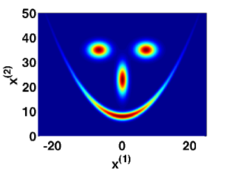
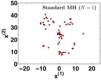
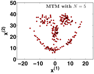
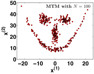
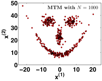
Figure 4: (a) The Smiling-Face target density. The remaining figures (b)-(c)-(d)-(e) depict the first $500$ generated samples drawn from the different samplers in one run (with $\sigma_{p}=10$). Note that the number of points are less than $500$ since, in certain iterations, the chain remains in the same state (depending on the acceptance probability $\alpha$) so that some points are repeated. (b) Samples generated by a standard MH ($N=1$). (c) Samples generated by a MTM with $N=5$. (d) Samples generated by a MTM with $N=100$. (e) Samples generated by a MTM with $N=1000$. It is evident that the MTM scheme speeds up the convergence of the Markov chain.

To draw from $p_{o}({\bf x})$, we apply a MH and a MTM scheme using for both a random walk Gaussian proposal pdf, i.e.,

$$\pi({\bf x}_{t}|{\bf x}_{t-1})\propto\exp\left\{-\left(x^{(1)}_{t}-x^{(1)}_{t-1}\right)^{2}/(2\sigma_{p}^{2})-\left(x^{(2)}_{t}-x^{(2)}_{t-1}\right)^{2}/(2\sigma_{p}^{2})\right\}.$$

In order to show the speed of the convergence of the samplers, we have generated only $500$ samples with a MTM with different number of candidates $N=1,5,100,1000$ (note with $N=1$ is a standard MH) and different standard deviation $\sigma_{p}=5,10$ of the proposal.

Tables 9-10 provide the average acceptance probability of a new state in the first column (the averaged values of $\alpha$), the jump rate among different modes in the second column (from “left eye” to the “smile”, or from the “smile” to the “nose” etc.) and the linear correlation for each component of ${\bf x}$, in the last column. To compute the mode-jump rate we establish that the state ${\bf x}_{t}$ belongs to the mode $i^{*}$ if

$$i^{*}=\arg\max_{i\in\{1,...,4\}}p_{i}({\bf x}_{t}),$$

where $p_{i}({\bf x}_{t})$ are the $4$ components in the mixture of Eq. (20). All results are averaged over $2000$ runs using $\sigma_{p}=5$ in Table 9 and $\sigma_{p}=10$ in Table 10.

Table 9: Numerical results with $\sigma_{p}=5$.

Number of tries $N$	Acceptance Rate	Mode-Jump Rate	Correlation
$N=1$ (standard MH)	0.2296	0.0401	$x^{(1)}\rightarrow$ 0.9460
			$x^{(2)}\rightarrow$ 0.9749
$N=5$	0.5118	0.1166	$x^{(1)}\rightarrow$ 0.8661
			$x^{(2)}\rightarrow$ 0.9492
$N=100$	0.7137	0.3373	$x^{(1)}\rightarrow$ 0.6193
			$x^{(2)}\rightarrow$ 0.8508
$N=1000$	0.7919	0.4430	$x^{(1)}\rightarrow$ 0.4724
			$x^{(2)}\rightarrow$ 0.7662

Table 10: Numerical results with $\sigma_{p}=10$.

Number of tries $N$	Acceptance Rate	Mode-Jump Rate	Correlation
$N=1$ (standard MH)	0.1464	0.0598	$x^{(1)}\rightarrow$ 0.9097
			$x^{(2)}\rightarrow$ 0.9653
$N=5$	0.4207	0.2313	$x^{(1)}\rightarrow$ 0.7536
			$x^{(2)}\rightarrow$ 0.8454
$N=100$	0.7670	0.5020	$x^{(1)}\rightarrow$ 0.3570
			$x^{(2)}\rightarrow$ 0.4607
$N=1000$	0.8930	0.6520	$x^{(1)}\rightarrow$ 0.1635
			$x^{(2)}\rightarrow$ 0.1453

From the tables, we can observe that the MTM clearly outperforms the standard MH since, as $N$ grows, the correlation decreases and the mode-jump rate increases (as does the acceptance rate) regardless of the chosen parameter $\sigma_{p}$ of the proposal. Obviously, the mode-jump rate is always less than the average value of the probability $\alpha$ of accepting a movement (the acceptance rate), since the mode-jumps represent a subset of all accepted movements. Moreover, the standard deviation $\sigma_{p}=10$ of the proposal pdf works better for the MTM method. In general, the MTM schemes work better with huge scaling parameters and a great-enough number of candidates $N$ (see also the discussion in the next section).

Figures 4(b)-(c)-(d)-(e) depict generated samples over one run. Clearly, in general we observe less than $500$ points since in certain cases a new movement is rejected and the chain remains in the same state. Namely, certain points are repeated. This effect is evident with the standard MH ($N=1$) whereas it vanishes as the number of candidates $N$ grows. Moreover, with greater $N$, the number of jumps among different modes also increases quickly. As a consequence, with the MTM technique ($N=5,100,1000$) all the features of the “face” (our target pdf) are completely described since the convergence of the chain is clearly speeded up. Therefore, with this numerical example, the main advantage of an MTM method becomes apparent: it can explore a larger portion of the sample space without a decrease of the acceptance rate, or even an increase thereof.

7 Discussion

In this work, we have studied the flexibility in the design of MTM techniques. We have introduced an MTM with generic weight functions (the analytic form can be chosen arbitrarily) and different proposal densities (each candidate can be drawn from a different pdf) combining the algorithms in [4] and [22]. Moreover, we have proposed a general framework for construction of acceptance probabilities in the MTM schemes, providing also specific examples. Finally, we have also designed a MTM algorithm without the need of generating randomly the reference points [26]. We have proved that the novel techniques satisfy the detailed balance condition, and carried out numerical simulations. Observing the theoretical workings and the numerical results, we can infer the following conclusions and observations:

1. General considerations: The classical MTM method, proposed in [17], clearly outperforms the standard MH algorithm using the same proposal pdf, in the sense that as the number of candidates increases, $N\rightarrow\infty$, then the correlation decreases quickly to zero (see Section 6.3 for further considerations). If a designed MTM scheme does not fulfill this property, then it is totally useless since the computational cost increased but the performance is not improved. Suitable MTM methods can be applied efficiently to any kind of target distributions (bounded or unbounded, with heavy tails or not), as shown in our numerical simulations (see Section 6.4). Moreover, the advantages of using an MTM technique w.r.t. a standard MH algorithm clearly grow as the dimensionality of the target increases.

2. MTM schemes as black-box algorithms: the numerical simulations show that, with a suitable number of tries $N$, the MTM methods provide good results independently of the choice of the parameters of the proposal. Therefore, it is important to remark that, even if no information about the target is available (for instance, about the location of the modes), an MTM scheme allows the use of a proposal pdf with a huge scaling parameter in order to explore quickly different regions of the space. Indeed, using a great-enough number of tries, this black-box approach is quite robust and always gives satisfactory performance. On other hand, with a huge scaling parameter, a standard MH usually produces a very small rate of jumps and, as a consequence, a very high correlation.

3. Choice of the weights: the possibility to choose any bounded and positive weight functions makes the MTM scheme easier to be designed since the user should not check any conditions to use suitable weights (as to check symmetry of the function $\lambda$, for instance) independently of the choice of the proposal pdfs. Namely, the proposal distribution and the weight functions can be selected separately, to fit well to the specific problem and to improve the performance of the technique. Note that, in some MTM approaches the symmetry condition of the function $\lambda$ can be complicated, see for instance [18, 24].

   Further theoretical or numerical studies are needed to determine the best choice of weight functions given a certain proposal and target density. We find that the weights of the analytic form proposed in [17] (see for instance Eq. (4)) usually provide better results. Within this class, the importance weights $\omega_{i}(y_{i})=\frac{p(y_{i})}{\pi_{i}(y_{i}|x)}$, based on the importance sampling principle [16, 25], appear to be a good choice in theory. Numerical results also suggest that weights simply proportional to the target density $\omega_{i}(y_{i})=p(y_{i})$ can provide good performance. In [2] the authors note that importance weights place higher probability on selecting candidates that are further away from the current state of the chain, but finally they prefer to use weights proportional to the target density based on numerical results.

   If the evaluation of the target $p(x)$ is computationally expensive such that the target function can not be included in the calculations of the weights, then the weight functions of the analytic class $\omega_{i}(y_{i},x)=p(y_{1})\pi_{i}(x|y_{i})\lambda(x,y_{i})$ proposed in [17] cannot be used. Indeed, it is impossible to find a symmetric function $\lambda(x,y)=\lambda(y,x)$ in order to remove the dependence on $p(x)$ in the weights (in this case there is just one possibility that $p(x)$ is constant, i.e., $p(x)=p(y)$ for all $x,y\in\mathcal{D}$). In this case, a possible choice of the weights can be proportional to the proposal pdfs, namely $w(y_{i})=\pi(x|y_{i})$ for instance. Clearly, it is not the optimal choice but, also in this case, the MTM can help to explore easily a larger portion of the sample space w.r.t. standard MH (see Section 6.2).

4. Use of different proposal pdfs: a MTM scheme with different proposal densities can be a very powerful framework mainly to tackle applications with high dimensionality and target distributions with several modes. In our opinion, the most promising scenario is to use different independent proposal distributions updating certain parameters (as mean and variance) each iteration of the chain, or selecting the best proposal among a set of functions (see Section 6.3 for further considerations). In this adaptive framework, the independent proposal pdfs could improved to fit better w.r.t. the target. This scheme has not been already exploited completely. It is important to remark that, in order to obtain a fair comparison among the generated candidates, it is recommendable to use proposal functions with the same area below, for instance they can be normalized.

5. Flexibility of the acceptance probabilities: we have shown there are certain freedom degrees in the design of an MTM algorithm, specifically in the choice of the acceptance probability $\alpha$. This is also confirmed by other works in literature that design suitable MTM schemes with correlated candidates but they are quite different (the strategies in [18, 24] generate the candidates sequentially, whereas the approach in [5] uses a block philosophy). However, although the detailed balance condition is always satisfied in all cases, the performance is different. Numerical results suggest that $\alpha$ functions as close as possible to the standard MTM method [17], using also the weights of the analytic form in Eq. (4), perform better results. Similar considerations can be done about the standard MH algorithm [1, 13, 23].

6. Reference points: we have described a possible MTM algorithm without drawing reference points. As seen in the numerical results, in this case it seems to exist an optimal value of the number of candidates $N$. As $N\rightarrow\infty$ the performance becomes very poor. Therefore, we can figure out that the “secret” of the good performance of the standard MTM scheme in [8, 17] is contained in the random generation of the reference points. However, there exists an important special case where the reference points are completely unnecessary: using independent proposal densities. In this case, the reference points can be set deterministically, equal to the previous generated candidates. This scheme, using just one proposal (drawing $N$ candidates from the same pdf) jointly with importance weights, appears as the easiest and natural procedure to combine the classical MH algorithm and importance sampling [25] (see Figure 3(a)).

7. Number of candidates: All the schemes proposed in literature and also in this work use a fixed number of candidates $N$. An important improvement would consist on tuning adaptively the number $N$ depending on the discrepancy between target and proposal distributions. To do this, a certain measure is needed, for instance, as the effective sample size of the importance sampling framework [16, 25]. Clearly, this idea could be more effective using independent proposal pdf since it is necessary to measure the discrepancy between the proposal and the target functions (with a random walk, for instance, the mean of the proposal changes each step and the distance w.r.t. the target varies as well). Another possibility could be to combine MTM and the delayed rejection method [21, 30]. With this kind of procedures, the optimal trade off between computational cost and performance would be achieved.

8 Acknowledgments

We would like to thank the Reviewers for their comments which have helped us to improve the first version of manuscript. Moreover, this work has been partially supported by Ministerio de Ciencia e Innovaci n of Spain (project MONIN, ref. TEC-2006-13514-C02- 01/TCM, Program Consolider-Ingenio 2010, ref. CSD2008- 00010 COMONSENS, and Distribuited Learning Communication and Information Processing (DEIPRO) ref. TEC2009-14504-C02-01) and Comunidad Autonoma de Madrid (project PROMULTIDIS-CM, ref. S-0505/TIC/0233).

References

- [1] A. A. Barker. Monte Carlo calculations of the radial distribution functions for a proton-electron plasma. Australian Journal of Physics, 18:119–133, 1965.
- [2] M. Bédard, R. Douc, and E. Mouline. Scaling analysis of multiple-try MCMC methods. Stochastic Processes and their Applications, 122:758–786, 2012.
- [3] S. P. Brooks. Markov Chain Monte Carlo method and its application. Journal of the Royal Statistical Society. Series D (The Statistician), 47(1):69–100, 1998.
- [4] R. Casarin, R. V. Craiu, and F. Leisen. Interacting multiple try algorithms with different proposal distributions. Statistics and Computing, pages 1–16, December 2011.
- [5] R. V. Craiu and C. Lemieux. Acceleration of the Multiple-Try Metropolis algorithm using antithetic and stratified sampling. Statistics and Computing, 17(2):109–120, 2007.
- [6] L. Devroye. Non-Uniform Random Variate Generation. Springer, 1986.
- [7] W. J. Fitzgerald. Markov Chain Monte Carlo methods with applications to signal processing. Signal Processing, 81(1):3–18, January 2001.
- [8] D. Frenkel and B. Smit. Understanding molecular simulation: from algorithms to applications. Academic Press, San Diego, 1996.
- [9] D. Gamerman. Markov Chain Monte Carlo: Stochastic Simulation for Bayesian Inference. Chapman and Hall/CRC, 1997.
- [10] W.R. Gilks, S. Richardson, and D. Spiegelhalter. Markov Chain Monte Carlo in Practice: Interdisciplinary Statistics. Taylor & Francis, Inc., UK, 1995.
- [11] H. Haario, E. Saksman, and J. Tamminen. Adaptive proposal distribution for random walk Metropolis algorithm. Computational Statistics, 14:375–395, 1999.
- [12] H. Haario, E. Saksman, and J. Tamminen. An adaptive Metropolis algorithm. Bernoulli, 7(2):223–242, April 2001.
- [13] W. K. Hastings. Monte Carlo sampling methods using Markov chains and their applications. Biometrika, 57(1):97–109, 1970.
- [14] S. Lan, V. Stathopoulosy, B. Shahbaba, and M. Girolami. Langrangian dynamical Monte Carlo. arXiv:1211.3759v1, November 2012.
- [15] F. Liang, C. Liu, and R. Caroll. Advanced Markov Chain Monte Carlo Methods: Learning from Past Samples. Wiley Series in Computational Statistics, England, 2010.
- [16] J. S. Liu. Monte Carlo Strategies in Scientific Computing. Springer, 2004.
- [17] J. S. Liu, F. Liang, and W. H. Wong. The Multiple-Try method and local optimization in Metropolis sampling. Journal of the American Statistical Association, 95(449):121–134, March 2000.
- [18] L. Martino, Victor Pascual Del Olmo, and Jesse Read. A multi-point Metropolis scheme with generic weight functions. Statistics & Probability Letters, 82(7):1445–1453, 2012.
- [19] L. Martino, J. Read, and D. Luengo. Improved adaptive rejection Metropolis sampling algorithms. arXiv:1205.5494v4, 2012.
- [20] N. Metropolis, A. Rosenbluth, M. Rosenbluth, A. Teller, and E. Teller. Equations of state calculations by fast computing machines. Journal of Chemical Physics, 21:1087–1091, 1953.
- [21] A. Mira. On Metropolis-Hastings algorithms with delayed rejection. Metron, 59:231–241, 2001.
- [22] Silvia Pandolfi, Francesco Bartolucci, and Nial Friel. A generalization of the Multiple-try Metropolis algorithm for Bayesian estimation and model selection. Journal of Machine Learning Research (Workshop and Conference Proceedings Volume 9: AISTATS 2010), 9:581–588, 2010.
- [23] P.H. Peskun. Optimum Monte-Carlo sampling using Markov chains. Biometrika, 60(3):607–612, 1973.
- [24] Z. S. Qin and J. S. Liu. Multi-Point Metropolis method with application to hybrid Monte Carlo. Journal of Computational Physics, 172:827–840, 2001.
- [25] C. P. Robert and G. Casella. Monte Carlo Statistical Methods. Springer, 2004.
- [26] C.P. Robert. “Xi’ An’s Og, an attempt at bloggin… ” Blog (by Christian P. Robert). http://xianblog.wordpress.com/2012/01/23/multiple-trypoint-metropolis-algorithm/, January 2012.
- [27] G. O. Roberts, A. Gelman, and W. R. Gilks. Weak convergence and optimal scaling of random walk Metropolis algorithms. Annals of Applied Probability, 7:110–120, 1997.
- [28] G. Storvik. On the flexibility of Metropolis-Hastings acceptance probabilities in auxiliary variable proposal generation. Scandinavian Journal of Statistics, 38(2):342–358, February 2011.
- [29] L. Tierney. Markov chains for exploring posterior distributions. Ann. Statist., 33:1701–1728, 1994.
- [30] L. Tierney and A. Mira. Some adaptive Monte Carlo methods for Bayesian inference. Stat. Med., 18:2507–2515, 1999.
- [31] Y. Zhang and W. Zhang. Improved generic acceptance function for multi-point Metropolis algorithm. 2nd International Conference on Electronic and Mechanical Engineering and Information Technology (EMEIT-2012), 2012.