The alpha effect in a turbulent liquid-metal plane Couette flow

Abstract

We calculate the mean electromotive force in plane Couette flows of a nonrotating conducting fluid under the influence of a large-scale magnetic field for driven turbulence. A vertical stratification of the turbulence intensity results in an $\alpha$ effect owing to the presence of horizontal shear. Here we discuss the possibility of an experimental determination of the components of the $\alpha$ tensor using both quasilinear theory and nonlinear numerical simulations. For magnetic Prandtl numbers of the order of unity, we find that in the high-conductivity limit the $\alpha$ effect in the direction of the flow clearly exceeds the component in spanwise direction. In this limit, $\alpha$ runs linearly with the magnetic Reynolds number $\rm Rm$ while in the low-conductivity limit it runs with the product $\rm Rm\cdot Re$, where $\rm Re$ is the kinetic Reynolds number so that for given $\rm Rm$ the $\alpha$ effect grows with decreasing magnetic Prandtl number.

For the small magnetic Prandtl numbers of liquid metals, a common value for the horizontal elements of the $\alpha$ tensor appears, which makes it unimportant whether the $\alpha$ effect is measured in the spanwise or streamwise directions. The resulting effect should lead to an observable voltage in both directions of about 0.5 mV for magnetic fields of 1 kgauss and velocity fluctuations of about 1 m/s in a channel of 50 cm height (independent of its width).

I Introduction

Mean-field electrodynamics of turbulent conducting fluids provides the commonly accepted approach to explaining the existence of magnetic fields of cosmic bodies. The excitation of magnetic fields results from the interplay of two elementary processes, diffusive and non-diffusive ones. It is known that turbulent motions reduce large-scale electric currents by inducing an electromotive force (EMF) opposite to the direction of the current. One can write

$$\overline{\mbox{\boldmath$u$}\times\mbox{\boldmath$b$}}=-\mu_{0}\eta_{\rm T}\overline{\mbox{\boldmath$J$}},$$ (1)

where $\mbox{\boldmath$\cal E$}=\overline{\mbox{\boldmath$u$}\times\mbox{\boldmath$b$}}$ is the EMF with $\mbox{\boldmath$u$}={\bm{U}}-\overline{\mbox{\boldmath$U$}}$ and $\mbox{\boldmath$b$}={\bm{B}}-\overline{\mbox{\boldmath$B$}}$ being the fluctuating contributions to velocity ${\bm{U}}$ and magnetic field ${\bm{B}}$, respectively, overbars denote averaging (to be specified later), $\mu_{0}$ is the vacuum permeability, ${\bm{J}}={\rm rot}{\bm{B}}/\mu_{0}$ is the current density, and $\eta_{\rm T}$ is the turbulent magnetic diffusivity. In stellar convection zones, $\eta_{\rm T}$ exceeds the molecular (microphysical) value $\eta$ of the magnetic diffusivity by many orders of magnitudes.

In this paper the EMF is derived for a turbulent fluid in the presence of a mean shear flow $\overline{\mbox{\boldmath$U$}}$ and a uniform background field $\overline{\mbox{\boldmath$B$}}$. For a turbulent dynamo, the enhanced dissipation must be overcome by an induction process that does not run with the electric current. One also knows that under the influence of global rotation and a uniform magnetic field, anisotropic turbulence produces an EMF parallel to the field KR80 , i.e.

$$\overline{\mbox{\boldmath$u$}\times\mbox{\boldmath$b$}}=\alpha\overline{\mbox{\boldmath$B$}}-\dots.$$ (2)

Here, $\alpha$ is a pseudoscalar formed by the rotation vector $\Omega$ and the anisotropy direction $g$ with $\alpha\propto\mbox{\boldmath$g$}\cdot\mbox{\boldmath$\Omega$}$. Often, the anisotropy direction from the gradient of density stratification of the fluid is used, but it is also possible that an intensity gradient close to rigid boundaries forms the preferred direction.

The resulting dynamo equation in rotating and stratified plasma is KR80

$$\frac{\partial\mbox{\boldmath$\bar{B}$}}{\partial t}={\rm rot}\bigg{(}\alpha\mbox{\boldmath$\bar{B}$}-(\eta+\eta_{\rm T}){\rm rot}\mbox{\boldmath$\bar{B}$}\bigg{)},$$ (3)

which has non-decaying solutions if $\alpha$ exceeds a critical value (‘$\alpha^{2}$-dynamo’); see Ref. B05 for a review.

In many papers the presented concept of a turbulent dynamo has been applied to planets, stars, accretion disks, galaxies and galaxy clusters; see references in RH04 . Only very few papers, however, deal with an experimental confirmation of the validity of relations (1) and (2) in the laboratory. This is surprising given the astrophysical importance of Eq. (3) as a direct consequence of Eqs. (1) and (2), which characterizes the basic ingredients of electrodynamics in rotating turbulent fluid conductors. Generally, the validity of Eq. (1) is not seriously doubted. However, the existing laboratory experiments report an increase of the effective magnetic diffusivity by only a few percent St12 . This is because the molecular magnetic diffusivity is rather large and the turbulence not strong enough. This is an unfortunate situation as the eddy-concept of the effective dissipation in turbulent media governs much of cosmic physics from climate research, geophysics, to the theory of star formation and quasars.

An even more dramatic situation holds with respect to the $\alpha$ effect. There are one or two experiments on the basis of the idea that the $\alpha$ effect is essentially a measure of the swirl of the flow. It has been demonstrated that a fluid with imposed helicity (imposed by rigid, swirling channels), produces an EMF in the direction of an imposed field; see Refs. St67 ; St06 ; F08 . It is not yet shown, however, that a rotating fluid with helicity that is not imposed (but results from the global rotation of the fluid) leads to an observable $\alpha$ effect. In natural cosmic bodies, helicity is usually due to the interaction of rotating turbulence with density stratification. The aim of the present paper is to suggest such a more rigorous $\alpha$ effect experiment. As we shall demonstrate, the difficulties in such an experiment make it understandable that this has not yet been possible without the use of a prescribed helicity.

It is easy to see the general difficulty of performing $\alpha$ effect experiments. Using Eq. (2), the potential difference between the endplates of the container in the direction of the mean magnetic field is

$$\Delta\varPhi=\alpha\overline{B}H,$$ (4)

where $H$ is the distance between the endplates. Hence, for $H\simeq 100$ cm and $B\simeq 1000$ gauss (say) the potential difference is $\Delta{\varPhi}=1$ mV for $|\alpha|=1\,$cm/s. The maximum $\alpha$ value is of the order of $u_{\rm rms}$, hence $\Delta{\varPhi}\lower 1.72218pt\hbox{$\;\buildrel<\over{\scriptstyle\sim}\;$}u_{\rm rms}$ in mV. For $u_{\rm rms}\simeq 1$ cm/s the maximally induced potential difference is therefore 1 mV. A container of 5 cm radius rotating with 1 Hz has a linear outer velocity of more than 30 cm/s so that $u_{\rm rms}\simeq 1$ cm/s might be considered as a conservative estimate. We find as a necessary condition for any $\alpha$ experiment that one must be able to measure potential differences smaller than a few mV. The $\alpha$ experiment in Riga St67 worked with $B\simeq 1$ kgauss and velocities of the order of m/s, so that the $\Delta{\varPhi}$ exceeded 10 mV. This experiment, however, used a prescribed helical geometry to mimic the symmetry breaking between left- and right-handed helicities.

If the rotation is not uniform, the resulting shear induces toroidal magnetic fields so that for sufficiently strong shear the $\alpha$ effect can be rather small and still produce a dynamo (‘$\alpha\Omega$-dynamo’). It is well known that also turbulence in liquid metals subject to a plane shear flow (without rotation!) is able to work as a dynamo if the turbulence intensity is stratified in the direction orthogonal to the shear flow plane; see Ref. RK06 . The basic rotation may thus not be the only flow, whose influence enables the turbulence to generate global magnetic fields.

In the present paper, a plane Couette flow is considered to analyze the characteristic issues of the corresponding $\alpha$ effect and to design a possible experiment to measure its amplitude.

II The mean electromotive force

Consider a plane shear flow with uniform vorticity in the vertical $z$ direction, i.e.,

$${\bar{U}}_{y}=Sx,$$ (5)

where $S$ is the shear rate. The shear flow may exist in a turbulence field that does not possess anisotropy other than that induced by the shear (5) itself. The one-point correlation tensor is

$$Q_{ij}=\overline{u_{i}(\mbox{\boldmath$x$},t)u_{j}(\mbox{\boldmath$x$},t)}.$$ (6)

The correlation tensor may be constructed by a perturbation method. The fluctuating velocity field is represented by a series expansion,

$${\mbox{\boldmath$u$}}={\mbox{\boldmath$u$}}^{(0)}+{\mbox{\boldmath$u$}}^{(1)}+{\mbox{\boldmath$u$}}^{(2)}+...\ ,$$ (7)

where the upper index shows the order of the contributions in terms of the mean shear flow.

The zero-order term represents the ‘original’ isotropic turbulence, which is assumed as being not yet influenced by the shear. We denote the Fourier transform of the correlation tensor by a hat and define the spectral tensor for the original turbulence as

$$\hat{Q}_{ij}^{(0)}=\frac{E(k,\omega)}{16\pi k^{2}}\left(\delta_{ij}-\frac{k_{i}k_{j}}{k^{2}}\right),$$ (8)

where the positive-definite spectrum $E$ gives the intensity of isotropic fluctuations with

$$\overline{{\mbox{\boldmath$u$}^{(0)}}^{2}}=\int\limits_{0}^{\infty}\!\!\int\limits_{0}^{\infty}E(k,\omega)\ {\rm d}k\ {\rm d}\omega.$$ (9)

Here, $k$ and $\omega$ are wavevector and frequency. For analytical calculations, the one-parametric spectrum

$$E(k,\omega)=\frac{2}{\pi}\frac{w}{\omega^{2}+w^{2}}\hat{E}(k),$$ (10)

can be used, which yields a $\delta$ function, $E\propto\delta(\omega)$, in the limit of $w\rightarrow 0$ and it leads to a white noise spectrum for large $w$. The correlation time of the turbulence is defined as $\tau_{\rm corr}=1/w$. The extremely short correlation times of white noise automatically lead to the high-conductivity limit for all fluid conductors with finite magnetic diffusivity $\eta$. On the other hand, the application of (10) in form of a $\delta$ function provides the result in the low-conductivity limit.

By definition, the magnetic diffusivity tensor relates the mean electromotive force (1) to gradients of the mean magnetic field via the relation ${\cal E}_{i}=\eta_{ijk}\bar{B}_{j,k}$. This tensor for originally isotropic turbulence, influenced by a mean shear flow (5), has been constructed up to the first order in the shear RK06 ; RS06 . In that work, it was also shown that the combination of shear and the shear-induced parts of the magnetic diffusion tensor are not able to operate as a dynamo.

On the other hand, it has been shown in Ref. RK06 that shear, in combination with stratified turbulence, provides helicity that leads to an $\alpha$ effect in Eq. (2). Here, $\alpha$ must be a pseudotensor so that an $\epsilon$ tensor has to appear in the coefficients for $\alpha$. The construction of the EMF, ${\cal E}_{i}=\epsilon_{ijk}\overline{u_{j}b_{k}}$, is the only possibility for the $\epsilon$ tensor to appear. The subscript of ${\cal E}_{i}$ is therefore always also a subscript of the $\epsilon$ tensor. As the $\epsilon$ tensor is of rank 3, an inhomogeneity of turbulence with the stratification vector $\mbox{\boldmath$g$}=\mbox{\boldmath$\nabla$}{}\log u_{\rm rms}^{2}$ and $u_{\rm rms}=\sqrt{\overline{u^{2}}}$, must also be present for the $\alpha$ effect to exist. If shear is included to first order, the general structure of the $\alpha$ tensor is

$$\alpha_{ij}\!\! = \!\!\gamma\epsilon_{ijk}g_{k}+\big{(}\alpha_{1}\epsilon_{ikl}\bar{U}_{j,k}+\alpha_{2}\epsilon_{ikl}\bar{U}_{k,j}\big{)}g_{l}+$$ (11)

$$+ \!\!\alpha_{3}\epsilon_{ikl}g_{j}\bar{U}_{l,k}+\alpha_{4}\epsilon_{ikj}\bar{U}_{l,k}g_{l}+\alpha_{5}\epsilon_{ijk}\bar{U}_{k,l}g_{l}.$$

If the stratification is along the vertical $z$ axis, it follows from (11) for the horizontal components of the $\alpha$ tensor that

$$\alpha_{xx} = \alpha_{2}g_{z}S=\alpha_{x}S,$$

$$\alpha_{yy} = -\alpha_{1}g_{z}S=\alpha_{y}S,$$

$$\alpha_{xy} = -\alpha_{yx}=\gamma g_{z}=\Gamma.$$ (12)

Turbulent pumping is characterized by $\alpha_{xy}$. The anisotropy of the $\alpha$ tensor is described by the difference between $\alpha_{x}$ and $\alpha_{y}$. In the adopted geometry, the azimuthal component $\alpha_{yy}$ (the coefficient $\alpha_{1}$ defined below) plays the main role in all cosmic applications, while in the proposed experiment with a turbulent shear flow the coefficient $\alpha_{2}$ is probed, and it produces the EMF perpendicular to the flow.

The coefficients in (12) read

$$\gamma=\frac{1}{6}\int\limits_{0}^{\infty}\!\!\int\limits_{0}^{\infty}\frac{\eta k^{2}E(k,\omega)}{\omega^{2}+\eta^{2}k^{4}}{\rm d}k\ {\rm d}\omega$$ (13)

for the pumping term and

$$\alpha_{n}=\int\limits_{0}^{\infty}\!\!\int\limits_{0}^{\infty}A_{n}E\left(k,\omega\right){\rm d}k\ {\rm d}\omega,$$ (14)

for the $\alpha$ effect with

$$A_{1} = \frac{4\nu\eta^{3}k^{8}+2\omega^{2}\eta\left(\nu+\eta\right)k^{4}}{15\left(\omega^{2}+\nu^{2}k^{4}\right)\left(\omega^{2}+\eta^{2}k^{4}\right)^{2}}+$$

$$+ \frac{\eta^{2}k^{4}\left(\eta^{2}k^{4}-3\omega^{2}\right)}{15\left(\omega^{2}+\eta^{2}k^{4}\right)^{3}},$$

$$A_{2} = -\frac{\eta^{2}\nu^{3}\left(4\eta-5\nu\right)k^{12}}{60\left(\omega^{2}+\nu^{2}k^{4}\right)^{2}\left(\omega^{2}+\eta^{2}k^{4}\right)^{2}}-$$ (15)

$$- \frac{\omega^{2}\nu\left(28\eta^{3}-4\eta^{2}\nu+12\eta\nu^{2}+5\nu^{3}\right)k^{8}}{60\left(\omega^{2}+\nu^{2}k^{4}\right)^{2}\left(\omega^{2}+\eta^{2}k^{4}\right)^{2}}-$$

$$- \frac{\omega^{4}\eta\left(\eta+36\nu\right)k^{4}-5\omega^{6}}{60\left(\omega^{2}+\nu^{2}k^{4}\right)^{2}\left(\omega^{2}+\eta^{2}k^{4}\right)^{2}}$$

for the kernels. Here, $\nu$ is the kinematic viscosity. In the following we define the magnetic Prandtl number as ${\rm Pm}=\nu/\eta$. Only the terms occurring in (12) have been given. For small ${\rm Pm}$, one can easily estimate the coefficient $\alpha_{1}$. For $\nu\ll\eta$, the expression for $A_{1}$ simplifies to

$$A_{1} = \frac{1}{15}\frac{1}{\left(\omega^{2}+\eta^{2}k^{4}\right)^{2}}\Bigg{\{}\frac{4\nu\eta^{3}k^{8}}{\omega^{2}+\nu^{2}k^{4}}+$$ (16)

$$+ \frac{\eta^{2}k^{4}\left(3\eta^{2}k^{4}-\omega^{2}\right)}{\omega^{2}+\eta^{2}k^{4}}\Bigg{\}}.$$

For $\nu\to 0$, the first expression on the RHS forms a $\delta$ function. Hence,

$$\alpha_{1}=\frac{2\pi}{15}\int\limits_{0}^{\infty}\!\!\frac{E(k,0)}{\eta k^{2}}{\rm d}k+\dots\simeq\frac{2\pi}{15}{\rm Rm}\ \ell_{\rm corr}^{2}+\dots,$$ (17)

with the magnetic Reynolds number of the turbulence

$${\rm Rm}=\frac{u_{\rm rms}^{2}\tau_{\rm corr}}{\eta}.$$ (18)

The missing terms in (17), however, are of the same order as the given one, so that it can only be used for orientation. In (17) we have used the estimate

$$\int\limits_{0}^{\infty}\!\!\frac{E(k,0)}{k^{2}}{\rm d}k=\tau_{\rm corr}u^{2}_{\rm rms}\ell_{\rm corr}^{2},$$ (19)

which follows from (10).

As mentioned above, the white-noise approximation mimics the high-conductivity limit, which holds for cosmic applications. In this approach, the spectrum does not depend on the frequency $\omega$ up to a maximum value $\omega_{\rm max}$, above which the power spectrum vanishes. This corresponds to a turbulence model with very short correlation time, i.e., $\tau_{\rm corr}\simeq 1/\omega_{\rm max}$. One finds from (16) after integration

$$\alpha_{1}=\frac{\pi}{6\eta}\int\limits_{0}^{\infty}\!\!\frac{E(k,0)}{k^{2}}{\rm d}k,$$ (20)

so that

$$\alpha_{1}=\frac{\pi}{6}{\rm Rm}\ \ell_{\rm corr}^{2},$$ (21)

which is similar to the result (17). The factor $\pi/6$ also appears in Fig. 1 for small $\rm Pm$ as the value of $I_{1}$ at the left vertical axis for $\tau_{\rm corr}=0$. The same procedure for $\rm Pm=1$, applied to (15)₁, leads to

$$\alpha_{1}=\frac{\pi}{15}{\rm Rm}\ \ell_{\rm corr}^{2}.$$ (22)

Now, one finds the factor $\pi/15$ on the left vertical axis of Fig. 1 (top) for $\rm Pm=1$. Note that the result for small $\rm Pm$ exceeds that for $\rm Pm=1$. For given $\eta$, smaller values of the viscosity $\nu$ lead to higher values of the EMF. It is this unexpected behavior that makes experiments with fluid metals with their small magnetic Prandtl numbers much-promising.

Figure 1: The numerical values of the coefficients $I_{1}$ and $I_{2}$. Top: $\rm Pm=1$, bottom: $\rm Pm=10^{-6}$. Note that in the high-conductivity limit ($\tau\to 0$, white noise spectrum) the coefficients $I_{1}$ and $I_{2}$ for $\rm Pm\ll 1$ exceed the values for $\rm Pm=1$. For small $\rm Pm$ the differences between $I_{1}$ and $I_{2}$ and the influence of the diffusivity parameter $\tau$ almost vanish.

Figure 2: $I_{1}$ for various $\rm Pm$. Obviously, for given magnetic diffusivity $\eta$ fluids with much smaller viscosity (like sodium and gallium) are even better qualified for laboratory experiments.

While very small values of $\tau_{\rm corr}$ (relative to the magnetic diffusion time $\tau_{\rm diff}$) represent the high-conductivity limit, a much larger value of $\tau_{\rm corr}$ represents the low-conductivity limit, which can be treated by assuming $w\to 0$ in Eq. (10), which corresponds to using a $\delta$ function in Eqs. (15). It directly follows from (15)₁ that

$$\alpha_{1}=\frac{1}{15}\left(1+\frac{4}{\rm Pm}\right){\rm Rm}^{2}\ \ell_{\rm corr}^{2},$$ (23)

so that $\rm Pm=1$ leads to $\alpha_{1}=\frac{1}{3}{\rm Rm}^{2}\ \ell_{\rm corr}^{2}$. For small magnetic Prandtl number one finds $\alpha_{1}=\frac{4}{15}{\rm Re}\ {\rm Rm}\ \ell_{\rm corr}^{2},$ where $\rm Re=Rm/Pm$ is the Reynolds number. Hence, in the low-conductivity limit (small $\rm Rm$) the $\alpha$ effect runs with $\rm Re\cdot Rm$, while in the high-conductivity limit (large $\rm Rm$) the $\alpha$ effect runs with $\rm Rm$. Very similar expressions also occur if the shear flow is formally replaced by a basic rotation Rue78 .

The general expression for finite correlation times, which is valid between the high and low conductivity limits, might also be written in the form

$$\alpha_{1}=I_{1}(\tau)\ {\rm Rm}\ \ell_{\rm corr}^{2},$$ (24)

where $I_{1}(\tau)$ is given in Fig. 1. This is the result of a numerical integration using a spectral function of the form ${\rm exp}(-\tau^{2}\omega^{2})$ with the dimensionless parameter

$$\tau=\eta k^{2}\tau_{\rm corr}\simeq 1/{\rm Rm},$$ (25)

for the aforementioned ratio of the correlation time to the magnetic diffusion time of the eddies. $\tau<1$ gives the sector of high conductivity and $\tau>1$ gives the sector of low conductivity. One finds that for the given range of $\tau$ for small $\rm Pm$, the function $I_{1}$ is nearly uniform (in contrast to the case of $\rm Pm=1$). The consequence is that, also for lower conductivity, the $\alpha$ effect only sinks linearly with $\rm Rm$ rather than quadratically as it is the case for $\rm Pm=1$. The appearance of the $1/{\rm Pm}$-term in Eq. (23) is the formal reason for this surprising and much-promising behavior.

As a demonstration, Fig. 2 shows the behavior of the numerical integrals for decreasing $\rm Pm$ and very large values of $\tau$. The integrals are running with $({\rm Pm}\ \tau)^{-1}$ so that for ${\rm Pm}\ \tau\gg 1$ the relation $\alpha_{1}\propto{\rm Re\ Rm}$ results. For small $\rm Pm$, the kinetic Reynolds number is much larger than the magnetic Reynolds number. For given magnetic diffusivity, smaller values of the viscosity strongly enhance the resulting $\alpha$ effect.

In experiments with liquid metals, $\rm Rm$ is of the order of 0.1…1, so $\tau\simeq 1...10$. In this regime, and for small $\rm Pm$, the coefficient $I_{1}$ hardly changes with $\tau$ (see Fig. 1). Its approximate value is 0.4, which is very close to the value $\pi/6$ valid in the high-conductivity limit. The reason is that for small $\rm Pm$ the transition of $I_{1}$ to the low-conductivity limit only happens at rather high values of $\tau$ (Fig. 2). In this limit one finds a strong influence of the magnetic Prandtl number.

Similar calculations for $\alpha_{2}$ lead to

$$\alpha_{2}\simeq-I_{2}\ {\rm Rm}\ \ell_{\rm corr}^{2},$$ (26)

where $I_{2}$ is also plotted in Fig. 1. For $\tau$ of the order of unity and small $\rm Pm$, we find $I_{2}\lower 1.72218pt\hbox{$\;\buildrel<\over{\scriptstyle\sim}\;$}I_{1}\approx 0.4$, so

$$\alpha_{2}\simeq-0.4\ {\rm Rm}\ \ell_{\rm corr}^{2}.$$ (27)

In the low-conductivity limit ($\tau\gg 1$), we have

$$\alpha_{2}=-\frac{1}{60}\left(\frac{4}{\rm Pm}-5\right){\rm Rm}^{2}\ \ell_{\rm corr}^{2},$$ (28)

which changes its sign at $\rm Pm=0.8$ and yields for small $\rm Pm$

$$\alpha_{2}=-\frac{1}{15}{\rm Rm}\,{\rm Re}\ \ell_{\rm corr}^{2}=-\alpha_{1}.$$ (29)

Indeed, Fig. 1 shows that for large values of $\tau$ and $\rm Pm=1$, $I_{2}$ is negative (and small), but for $\rm Pm\ll 1$ it is positive ($\simeq 0.4$).

In summary, the plots in Fig. 1 reveal an important influence of the value of the viscosity on the $\alpha$ effect for a given diffusivity. For small $\rm Pm$, using the low-conductivity limit, the ratio of $I_{2}$ to $I_{1}$ approaches unity, while for $\rm Pm=1$ it is very small. Note that for $\rm Pm=1$, $\alpha_{1}$ strongly exceeds $\alpha_{2}$, but this is no longer the case for small $\rm Pm$. The two horizontal components of the $\alpha$ tensor are then of the same order of magnitude. The signs of the components are always identical.

It must also be mentioned that the magnetic Prandtl number is much smaller for liquid metals than what can presently be used in numerical simulations. Figure 1 shows that in numerical simulations, $\alpha_{xx}$ should be smaller than $\alpha_{yy}$, what is not true, however, for laboratory conditions with their small $\rm Pm$. In this case it does not matter whether the shear-induced $\alpha$ effect is measured in the streamwise or the spanwise direction.

This finding is in stark contrast to the results of the turbulence model described in Ki91 for applications to convection zones. This model works with a very steep frequency spectrum, $E\propto\delta(\omega)$, and assumes ${\rm Pm}=\tau=1$ for the diffusivities of a postulated small-scale background turbulence. This immediately leads to $A_{2}/A_{1}=1/20$, i.e., $\alpha_{xx}/\alpha_{yy}=1/20$. The considered turbulence model, therefore, yields a strongly dominating $\alpha$ effect in the azimuthal direction (as also in our approach for $\rm Pm=1$).

It is also obvious that the pumping term does not depend on the shear. After (13), for small $\eta$, it does not run with $1/\eta$. It is simply

$$\gamma\simeq u^{2}_{\rm rms}\tau_{\rm corr}\simeq\eta\ {\rm Rm}.$$ (30)

It can only be measured if the external field $B_{0}$ lies in the shear plane.

III Numerical simulations

It is straightforward to verify the existence of an $\alpha$ effect in a shear flow using numerical simulations of non-uniformly forced turbulent shear flows in Cartesian coordinates. We perform simulations in a cubic domain of size $L^{3}$, so the minimal wave number is $k\equiv k_{1}=2\pi/L$. We solve the equations of compressible hydrodynamics with an isothermal equation of state with constant sound speed $c_{\rm s}$,

$${{\rm D}{\bm{U}}\over{\rm D}t}=SU_{x}\hat{\bm{y}}-c_{\rm s}^{2}\mbox{\boldmath$\nabla$}{}\log\rho+{\bm{f}}+\rho^{-1}\mbox{\boldmath$\nabla$}{}\cdot 2\rho\nu\mbox{\boldmath${\sf S}$}{},$$ (31)

$${{\rm D}\log\rho\over{\rm D}t}=-\mbox{\boldmath$\nabla$}{}\cdot{\bm{U}},$$ (32)

where ${\rm D}/{\rm D}t=\partial/\partial t+{\bm{U}}\cdot\mbox{\boldmath$\nabla$}{}+Sx\;\partial/\partial y$ is the advective derivative with respect to the full velocity field (including the shear flow), ${\bm{U}}$ is the departure from the mean shear flow $(0,Sx,0)$, and ${\sf S}_{ij}={1\over 2}(\partial_{i}U_{j}+\partial_{j}U_{i})-{1\over 3}\delta_{ij}\mbox{\boldmath$\nabla$}{}\cdot{\bm{U}}$ is the trace-less rate of strain matrix (not to be confused with the shear rate $S$). The flow is driven by a random forcing function ${\bm{f}}$ consisting of non-helical waves with wave numbers whose modulus lie in a narrow band around an average wave number $k_{\rm f}=5k_{1}$ HBD04 . We arrange the amplitude of the forcing function such that the rms velocity increases with height, while the maximum Mach number remains below 0.1, so the effects of compressibility are negligible. The resulting flow is irregular in space and time and will loosely be referred to as turbulence.

We use the kinematic test-field method Sch07 in the Cartesian implementation BRRK08 to compute from the simulations simultaneously the relevant components of the $\alpha$ effect and turbulent diffusivity tensors, $\alpha_{ij}$ and $\eta_{ij}$. We do this by solving an additional set of equations governing the departure of the magnetic field from a set of given mean fields. This mean field is referred to as a test field and is marked by the superscript T. For each test field ${\overline{\mbox{\boldmath$B$}}}^{\rm T}$, we find the corresponding fluctuations ${{\bm{b}}^{\rm T}={\rm rot}{\bm{a}}^{\rm T}}$ by solving the inhomogeneous equation for the corresponding vector potential ${\bm{a}}^{\rm T}$,

$${{\cal D}{\bm{a}}^{\rm T}\over{\cal D}t}=-Sa_{y}^{\rm T}\hat{\bm{x}}+\overline{\mbox{\boldmath$U$}}\times{\bm{b}}^{\rm T}+{\bm{u}}\times{\overline{\mbox{\boldmath$B$}}}^{\rm T}+\left({\bm{u}}\times{\bm{b}}^{\rm T}\right)^{\prime}+\eta\nabla^{2}{\bm{a}}^{\rm T},$$ (33)

where ${\cal D}/{\cal D}t=\partial/\partial t+Sx\;\partial/\partial y$ is the advective derivative with respect to the imposed shear flow only (i.e., without ${\bm{U}}$), and ${\left({\bm{u}}\times{\bm{b}}^{\rm T}\right)^{\prime}={\bm{u}}\times{\bm{b}}^{\rm T}-\overline{{\bm{u}}\times{\bm{b}}^{\rm T}}}$ is the fluctuating part of ${\bm{u}}\times{\bm{b}}^{\rm T}$. We compute the corresponding mean electromotive force, ${\bm{{\cal E}}^{\rm T}=\overline{{\bm{u}}\times{\bm{b}}^{\rm T}}}$, which is then related to ${\overline{\mbox{\boldmath$B$}}}^{\rm T}$ and its curl, $\mu_{0}{\overline{\mbox{\boldmath$J$}}}^{\rm T}={\rm rot}{\overline{\mbox{\boldmath$B$}}}^{\rm T}$, via

$${\cal E}_{i}^{\rm T}=\alpha_{ij}{\overline{B}}^{\rm T}_{j}-\eta_{ij}\mu_{0}{\overline{J}}^{\rm T}_{j}.$$ (34)

We use 4 different test fields with $x$ or $y$ components being proportional to $\sin kz$ or $\cos kz$. The $x$ and $y$ components of Eq. (34) constitute then 8 equations for the 4 relevant components of $\alpha_{ij}(z,t)$ and $\eta_{ij}(z,t)$.

We adopt periodic boundary conditions in the $y$ direction, shearing–periodic boundary conditions in the $x$ direction, and stress-free perfect conductor boundary conditions in the $z$ direction, i.e.,

$$\partial_{z}u_{x}=\partial_{z}u_{y}=u_{z}={a}^{\rm T}_{x}={a}^{\rm T}_{y}=\partial_{z}{a}^{\rm T}_{z}=0.$$ (35)

Numerical resolutions of $64^{3}$ and $128^{3}$ mesh points were found to be sufficient, depending on the value of ${\rm Pm}$. The Pencil Code  pencil has been used for all calculations.

Simulations are performed for different parameter combinations. The quantities $S$ and $g_{z}$ are positive in the calculations presented here, i.e. the basic velocity (5) grows in the positive $x$ direction while the turbulence intensity grows in the positive $z$ direction. To make contact with laboratory experiments, we focus here on the case of low conductivity and choose ${\rm Rm}\equiv u_{\rm rms}/\eta k_{\rm f}=0.2$, which is consistent with our definition of Eq. (18) with a Strouhal number of unity, i.e. $\tau_{\rm corr}u_{\rm rms}k_{\rm f}=1$.

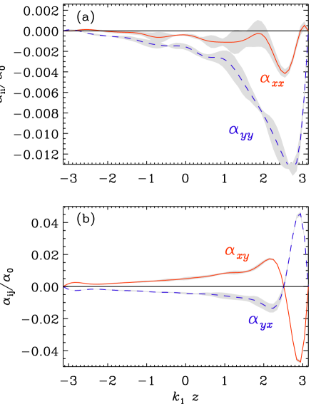
Figure 3: Simulations with positive shear ($s=0.2)$: The numerical values for the diagonal elements of the $\alpha$ tensor (top) and the off-diagonal elements (bottom). Error margins are indicated in gray. $\rm Pm=1$. $\rm Re=0.2$, $\rm Rm=0.2$.

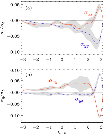
Figure 4: The same as in Fig. 3, but for $\rm Pm=0.1$. $\rm Re=2.5$, $\rm Rm=0.25$.

As in earlier work using fully helical turbulence, we present time averages of the components of $\alpha_{ij}$ and $\eta_{ij}$ in normalized form in terms of $\alpha_{0}=u_{\rm rms}/3$ and $\eta_{\rm T0}=u_{\rm rms}/3k_{\rm f}$. Hence, $\alpha_{0}\,L/\eta_{\rm T0}=Lk_{\rm f}=10\pi$. Error margins are estimated as the largest departure of any one third of the full times series of $\alpha_{ij}$ and $\eta_{ij}$. The shear of the background flow is normalized with the speed of sound, i.e.

$$S=sc_{\rm ac}k_{1}=\frac{2\pi su_{\rm rms}}{{\rm Ma}L},$$ (36)

where ${\rm Ma}=u_{\rm rms}/c_{\rm ac}$ is the Mach number. In the simulations we work with $s=0.2$ and $\rm Ma=0.05$. One finds

$$\frac{\alpha_{yy}}{\alpha_{0}}\simeq-\frac{\ell_{\rm corr}^{2}}{L^{2}}.$$ (37)

Following Eqs. (12), both streamwise and spanwise $\alpha$ tensor components, $\alpha_{yy}$ and $\alpha_{xx}$, should be negative. When the simulations are done for $\rm Pm=1$, $|\alpha_{yy}|$ should strongly exceed the value of $|\alpha_{xx}|$, but this is not expected for $\rm Pm<1$. Here, the results of two simulations are presented. The first one for $\rm Pm=1$ with $64^{3}$ meshpoints has $\rm Rm=0.2$ and $\rm Re\cdot Rm=0.04$, while the second one for $\rm Pm=0.1$ with $128^{3}$ meshpoints has $\rm Rm=0.25$ and $\rm Re\cdot Rm=0.625$. It is thus possible to find out whether the simulated $\alpha$ effect runs with $\rm Rm$ (which is almost the same) or with $\rm Rm\cdot Re$ (which differs by a factor of 10) in both simulations. In both cases $k_{\rm f}/k_{1}=5$ so that 10 cells can exist in the vertical direction and, therefore, $\ell_{\rm corr}^{2}/{L^{2}}\simeq 0.01$.

As predicted, Fig. 3(a) for $\rm Pm=1$ shows $\alpha_{yy}$ to be dominant and both diagonal components of $\alpha$ as basically negative. The amplitude of ${\alpha_{yy}}/\alpha_{0}$ is about 0.01 in accordance to Eq. (37) which also leads to $|\alpha_{yy}|/\alpha_{0}\simeq 0.01$.

For $\rm Pm=1$, $I_{2}$ is strongly reduced relative to $I_{1}$ so that the small amplitude of $\alpha_{xx}$ in Fig. 3(a) becomes understandable. For smaller magnetic Prandtl number, this reduction does not exist and both $\alpha$ components are of similar amplitude. Close to the upper endplate the intensity stratification changes its sign (due to the boundary conditions) and also a change of the sign of the $\alpha$ effect can be observed there (see Fig. 4)(a). Without this exception the simulations also confirm that the signs only depend on the sign of the product $g_{z}S$, as formulated in the relations (12).

Moreover, again as predicted, the amplitudes of the diagonal elements of the $\alpha$ tensor increase for decreasing magnetic Prandtl number. In the middle of the channel, the amplitudes of the $\alpha$ components differ by a factor of 10 which exceeds the ratio 1.25 of the two $\rm Rm$ by almost an order of magnitude.

Next, the off-diagonal components of $\alpha_{ij}$ are considered; see Figs. 3(b) and 4(b). As expected, we have $\alpha_{yx}\approx-\alpha_{xy}$, which corresponds to a turbulent pumping velocity in the $z$ direction. This velocity is negative for $k_{1}z<2.5$, corresponding to downward transport, i.e., down the gradient of the turbulent intensity, as expected KR80 . Near the top of the domain, the gradient of the turbulent intensity is reversed and so is the sign of the pumping velocity $\alpha_{yx}$. The simulations with $\rm Pm=0.1$ and $1$ lead to the result $\alpha_{yx}/\alpha_{0}\simeq-{\rm Rm}/10$ (Figs. 3b and 4b).

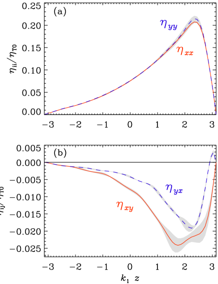
Figure 5: Simulations with $s=0.2$ for the shear-induced elements of the $\eta$ tensor. Top: the horizontal eddy diffusivities; bottom: the two shear–current terms $\eta_{xy}$ and $\eta_{yx}$. Error margins are indicated in gray. $\rm Pm=1$. $\rm Re=0.2$, $\rm Rm=0.2$.

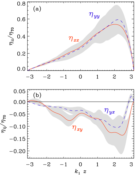
Figure 6: The same as in Fig. 5, but for $\rm Pm=0.1$. $\rm Re=2.5$, $\rm Rm=0.25$.

IV The diffusivity tensor

The numerical test-field procedure also allows the simultaneous calculation of the components of the $\eta$ tensor for the same simulation with its vertical stratification of the turbulence intensity. This knowledge is important for the discussion of the question whether turbulence in shear flows can be used for dynamo self-excitation of large-scale magnetic fields. Despite the completely different roles played by the spanwise and streamwise directions, we find the two relevant diagonal components of the diffusivity tensor to be nearly equal, i.e., $\eta_{xx}\approx\eta_{yy}$ (Figs. 5a and 6a). This strikingly high degree of isotropy of the turbulent diffusivity in the $xy$ plane has already been noticed in earlier simulations of the diffusivity in unstratified turbulent shear flows B05 ; RK06 ; BRRK08 . The maximum of $\eta_{\rm T}=(\eta_{xx}+\eta_{yy})/2$ is about 20% of the reference value $\eta_{0}$, which agrees with the fact that for ${\rm Rm}\ll 1$, $\eta_{\rm T}/\eta_{0}\simeq{\rm Rm}$ Sur . For larger $\rm Rm$ (or for smaller $\rm Pm$) one finds slightly larger numerical values for the eddy diffusivity (Fig. 6a).

The data in Figs. 3(a) to 6(a) for $\rm Pm=0.1$ and $1$ lead to a value of about unity for the normalized $\alpha$ effect, $C_{\alpha}=\alpha\,L/\eta_{\rm T}$, which is also typical for rapidly rotating convection KKB09 . A comparison with the slab-dynamo calculation in RK06 leads to $C_{\alpha}\simeq 10$ as required for self-excitation of the magnetic fields. This condition is not fulfilled for the present simulations.

For the off-diagonal components of the $\eta$ tensor for non-stratified shear flows one finds

$$\eta_{xy}=\eta_{x}S,\quad\eta_{yx}=\eta_{y}S,$$ (38)

i.e., both are linear in $S$. The calculation of a simple slab dynamo model shows self-excitation for sufficiently large positive $\eta_{y}$. From quasilinear theory we know, however, that $\eta_{y}$ is negative-definite RK06 . For positive shear, the coefficient $\eta_{yx}$ is therefore expected to be negative. This result has also been confirmed for ${\rm Rm}\leq 200$ for unstratified turbulence BRRK08 .

The same sign and the same linear dependence of $\eta_{yx}$ on $S$ also holds for $\eta_{xy}$, but only for $\rm Pm$ of order unity and in the low conductivity limit. Both conditions are fulfilled for the present simulations. Experiments for liquid metals, however, concern much smaller magnetic Prandtl numbers, for which $\eta_{xy}$ is expected to be positive.

Our numerical simulations for stratified turbulence and with positive shear and $\rm Pm\leq 1$ also produce negative values for both $\eta_{xy}$ and $\eta_{yx}$ (Figs. 5b and 6b). The possibility of dynamo action in such non-helical shear flows RK03 ; BRRK08 ; Yousef can therefore not be explained by the so-called shear–current effect.

It is also shown that the vertical stratification of the turbulence intensity does not basically modify the known findings about the eddy diffusivity tensor. Only experiments can finally provide the sign of $\eta_{x}$ as simulations for such small $\rm Pm$ are not usually possible.

V Shear flow electrodynamics

Following relations (12), the electromotive force across the channel is

$${\cal E}_{x}=\alpha_{2}g_{z}SB_{0},$$ (39)

so that the potential difference $\delta\varPhi$ between the walls with distance $D$ is $\delta\varPhi=\alpha_{2}g_{z}SDB_{0}$ so that

$$\delta\varPhi\simeq-0.5\,{\rm Rm}\,\ell_{\rm corr}^{2}g_{z}UB_{0}\simeq-{\rm Rm}\ \lambda^{2}\ LUB_{0}$$ (40)

with $I_{2}\simeq 0.5$ for small $\rm Pm$ (Fig. 1, bottom), with $g_{z}=2/L$ as the vertical scale height of the turbulence stratification and with the ratio $\lambda=\ell_{\rm corr}/L$. The amplitude of the mean shear flow is $U$. Note that surprisingly the width $D$ of the channel does not appear in (40) and even the height $L$ has only a weak influence. Hence,

$$\delta\varPhi\simeq 10\ {\rm Rm}\,\lambda^{2}\left[\frac{L}{10\,{\rm cm}}\right]\left[\frac{U}{{\rm m/s}}\right]\left[\frac{B_{0}}{\rm kgauss}\right]$$ (41)

(in mVolt) so that with (say) $\lambda\simeq 0.1$ and a channel height of 50 cm, a shear flow of 1 m/s subject to a magnetic field of 1 kgauss would lead to a potential difference of

$$\delta\varPhi\simeq 0.5\ {\rm Rm}\ [\rm mV].$$ (42)

For the (maximal) value of $\rm Rm\simeq 1$ ($u_{\rm rms}\simeq 1$m/s and $\ell_{\rm corr}\simeq 5$ cm) the channel should thus provide a potential difference of 0.5 mV between the side walls by the action of the $\alpha$ effect along a spanwise magnetic field. These numbers are quite similar to those of the Riga experiment St67 ; KR80 . The basic difference is that in our shear flow the helicity is not prescribed but it is self-consistently produced by the interaction of the stratified turbulence with the background shear.

VI Conclusions

Laboratory studies of homogeneous dynamos are still in their infancy. The only working dynamo where the flow pattern is not strongly constrained by pipes or container walls is the experiment in Cadarache Cada , where, however, the effects of soft iron play an important and not well understood role gies12 . The present proposal of measuring the $\alpha$ effect in an unconstrained turbulent flow would therefore be a major step forward. In such an experiment, the pseudoscalar necessary for producing helicity comes from the stratification of turbulent intensity giving rise to a polar vector and the vorticity associated with the shear flow giving rise to an axial vector. Thus, the basic effects in the theory of turbulent dynamos, which are usually considered as special properties of rotating and stratified fluids, can also be found for the plane-shear flows, i.e. without global rotation.

The present work yields a detailed prediction about the sign and magnitude of the components of both $\alpha$ and $\eta$ tensors. It may motivate the construction of a suitable experiment using liquid metals to achieve a measurable $\alpha$ effect. The necessary vertical stratification of turbulence intensity must be experimentally imitated using grids with nonuniform mesh sizes and/or walls of increasing/decreasing roughness in the vertical direction.

We have shown that in stratified turbulence driven in a plane shear flow, a measurable $\alpha$ effect should exist. Here, the key problem is the smallness of the magnetic Prandtl number. For $\rm Pm\leq 1$, the quasilinear theory and the possible nonlinear numerical simulations lead to very similar results. With the quasilinear theory we have shown that, even for fluids with very small magnetic Prandtl numbers, stratified shear flow turbulence leads to an $\alpha$ effect that can be realized in an experiment with liquid metals such as sodium ($\rm Pm\simeq 10^{-5}$) or gallium ($\rm Pm\simeq 10^{-6}$). Such small magnetic Prandtl numbers cannot be simulated with present-day numerical codes.

In fact, it may not be possible that such flows could produce a supercritical dynamo in the conceivable future. Nevertheless, even in the subcritical case, an $\alpha$ effect should be measurable, which would thus open the possibility of detailed comparisons between theory, simulations and experiments. Once such a comparison is possible, there will be more details that should be investigated. One of them concerns the modifications of the results in the presence of imperfect scale separation in space and time. For oscillatory dynamos, this effect can significantly lower the excitation conditions for the dynamo compared to standard mean-field estimates RB12 .

- (1) F. Krause and K.-H. Rädler, Mean-Field Magnetohydrodynamics and Dynamo Theory (Pergamon Press, Oxford, 1980).
- (2) A. Brandenburg, Astron. Nachr. 326, 787 (2005).
- (3) G. Rüdiger and R. Hollerbach, The Magnetic Universe: Geophysical and Astrophysical Dynamo Theory (Wiley-VCH, Berlin, 2004).
- (4) V. Noskov, S. Denisov, R. Stepanov, and P. Frick, Phys. Rev. E, 85, 016303 (2012).
- (5) M. Steenbeck, I. M. Kirko, A. Gailitis, A. P. Klawina, F. Krause, I. J. Laumanis, and O. A. Lielausis, Monats. Dt. Akad. Wiss. 9, 714 (1967).
- (6) R. Stepanov, R. Volk, S. Denisov, P. Frick, V. Noskov, and J.-F. Pinton, Phys. Rev. E 73, 046310 (2006).
- (7) P. Frick, S. Denisov, V. Noskov, and R. Stepanov, Astron. Nachr. 329, 706 (2009).
- (8) G. Rüdiger and L. L. Kitchatinov, Astron. Nachr. 327, 298 (2006).
- (9) M. Schrinner, K.-H. Rädler, D. Schmitt, M. Rheinhardt, and U. R. Christensen, Geophys. Astrophys. Fluid Dynam. 101, 81 (2007).
- (10) K.-H. Rädler and R. Stepanov, Phys. Rev. E 73, 056311 (2006).
- (11) G. Rüdiger, Astron. Nachr. 299, 217 (1978).
- (12) L. L. Kichatinov, Astron. Astrophys. 243, 483 (1991).
- (13) N. E. L. Haugen, A. Brandenburg, and W. Dobler, Phys. Rev. E 70, 016308 (2004).
- (14) A. Brandenburg, K.-H. Rädler, M. Rheinhardt, and P.J. Käpylä, Astrophys. J. 676, 740 (2008).
- (15) http://pencil-code.googlecode.com
- (16) S. Sur, A. Brandenburg, and K. Subramanian, Mon. Not. R. Astron. Soc. 385, L15 (2008).
- (17) P. Käpylä, M. Korpi, and A. Brandenburg, Astron. Astrophys. 500, 633 (2009).
- (18) T. A. Yousef, T. Heinemann, A. A. Schekochihin, N. Kleeorin, I. Rogachevskii, A.B. Iskakov, S. C. Cowley, and J. C. McWilliams, Phys. Rev. Lett. 100, 184501 (2008).
- (19) I. Rogachevskii and N. Kleeorin, Phys. Rev. E 68, 036301 (2003).
- (20) E. T. Vishniac and A. Brandenburg, Astrophys. J. 475, 263 (1997).
- (21) R. Monchaux, M. Berhanu, M. Bourgoin, M. Moulin, Ph. Odier, J. -F. Pinton, et al., Phys. Rev. Lett. 98, 044502 (2007).
- (22) A. Giesecke, C. Nore, F. Stefani, G. Gerbeth, et al., NJP 14, 3005 (2012).
- (23) M. Rheinhardt and A. Brandenburg, Astron. Nachr. 333, 80 (2012).