Finding the bare band: Electron coupling to two phonon modes in potassium-doped graphene on Ir(111)

Abstract

We analyze renormalization of the $\pi^{*}$ band of n-doped epitaxial graphene on Ir(111) induced by electron-phonon coupling. Our procedure of extracting the bare band relies on recursive self-consistent refining of the functional form of the bare band until the convergence. We demonstrate that the components of the self-energy, as well as the spectral intensity obtained from angle-resolved photoelectron spectroscopy (ARPES) show that the renormalization is due to the coupling to two distinct phonon excitations. From the velocity renormalization and an increase of the imaginary part of the self-energy we find the electron-phonon coupling constant to be $\sim 0.2$, which is in fair agreement with a previous study of the same system, despite the notable difference in the width of spectroscopic curves. Our experimental results also suggest that potassium intercalated between graphene and Ir(111) does not introduce any additional increase of the quasiparticle scattering rate.

I Introduction

Graphene is a fascinating two-dimensional material with linear electronic bands and linear dependence of the density of states around the Fermi level. (Castro Neto et al., 2009) By field-effect or chemical doping (either n or p) Fermi level can be tuned to change graphene from a zero-gap semiconductor to a metal. (Giovannetti et al., 2008; Coletti et al., 2010; Liu et al., 2011) Intrinsic and doped graphene prove to be an interesting platform to study different aspects of many-body interactions in two-dimensional systems, either experimentally (Bostwick et al., 2007, 2010; Siegel et al., 2011a) or theoretically (Das Sarma et al., 2007; Mak et al., 2011; Park et al., 2008a) . A particular accent is put on the electron-phonon coupling (EPC) in doped graphene. (Grüneis et al., 2009; Valla et al., 2009; Borysenko et al., 2010)

Adsorption and/or intercalation of alkali atoms in epitaxial graphenes can lead to a whole range of n dopings, including an extreme case where graphene’s van Hove point is brought to the Fermi level. (McChesney et al., 2010) Studies on KC₈ (Grüneis et al. (2009)) and CaC₆ (Valla et al. (2009)) report strong EPC anisotropy, with significantly smaller EPC constant $\lambda$ along the K-$\Gamma$, compared to the K-M direction. Despite the fact that these experiments were performed by intercalation of graphite, it had been demonstrated that the intercalation separates single layers of graphite in such a way that it shows all signatures of graphene. Some others have reported smaller value of $\lambda$,(Bianchi et al., 2010; Zhou et al., 2008; Siegel et al., 2011b) and no anisotropy in the EPC. (Bianchi et al., 2010) Recent results also suggest that EPC progressively increases with doping. (Pan et al., 2011)

Determination of the renormalization effects in n-doped $\pi^{*}$ band due to the EPC is complicated, in particular along the K-M direction, because of the non-linear behavior of the band close to the Fermi level. (Park et al., 2008b) A simple procedure to establish the strength of electron-phonon coupling by a comparison of the quasiparticle velocity at the Fermi level and the velocity well beyond the phonon energy scale is shown to be compromised by a significant change of the quasiparticle velocity due to the nonlinearity of the $\pi^{*}$ band. (Park et al., 2008b) Some other procedures rely on the bare-band dispersion. (Hofmann et al., 2009) The choice of the bare-band may, however, influence an accurate determination of the magnitude and shape of the self-energy. (Kordyuk et al., 2005) A self-consistent GW approximation was applied in ab-initio density functional theory (DFT) calculation to model graphene’s bare band that includes all electron-electron correlations. (Grüneis et al., 2009) In order to avoid any arbitrariness, determination of the bare band dispersion from the experimental data is desirable. Different approaches based on self-consistent procedures have been developed to determine the bare band, self-energy and ultimately, electron-phonon coupling strength. (Kordyuk et al., 2005; Veenstra et al., 2011; Bianchi et al., 2010)

A self-consistent method has already been applied to the photoemission data of potassium doped graphene on Ir(111). (Bianchi et al., 2010) Several aspects of the low-energy quasiparticle dynamics were addressed: renormalization of the $\pi^{*}$ band close to the Fermi level due to the coupling to phonons; phonon spectrum associated with the renormalization; the width of spectral lines in connection with the electron scattering rate. A model with a spectrum of five evenly spaced phonons participating in the coupling to graphene’s $\pi^{*}$ band was used in the self-energy analysis. The EPC constant was found relatively small (0.28) and isotropic around K. Rather broad peaks were interpreted in terms of an increased electron scattering rate caused by the loss of translation symmetry induced by the incommensurability of the system graphene/Ir(111). (Bianchi et al., 2010) An ARPES study on another metallic system — graphene on a copper foil — questions all previous findings, proposing an order of magnitude smaller electron-phonon coupling strength. (Siegel et al., 2011b)

In this paper we present results of an ARPES study of highly ordered graphene on Ir(111)(Kralj et al., 2011; Pletikosić et al., 2009) intercalated (Tontegode and Rut’kov, 1993) with potassium. We use maxima of momentum distribution curves (MDC) and energy distribution curves (EDC) to determine the exact dispersion of the $\pi^{*}$ band along the K-M direction. Peak positions and widths of MDCs are used in a self-consistent method to reconstruct the bare band $E_{b}$ and the corresponding $\mathfrak{Im}\Sigma(E)$ and $\mathfrak{Re}\Sigma(E)$. Both show, consistently with the spectral intensity $A(E)$, that the renormalization is due to the coupling to two distinct phonon excitations. From the velocity renormalization and an increase of $\mathfrak{Im}\Sigma(E)$ with energy electron-phonon coupling constant is determined.

II Method

Photoemission spectra offer a wealth of information about many-body interactions in solids, in particular two-dimensional ones. The single-particle spectral function, that the intensities in the photoemission spectra are proportional to, is given by:

$$A(k,E)=\frac{1}{\pi}\frac{\mathfrak{Im}\Sigma(E)}{[E-E_{b}(k)-\mathfrak{Re}\Sigma(E)]^{2}+[\mathfrak{Im}\Sigma(E)]^{2}}$$ (1)

Here, $E_{b}$ is the dispersion relation of the bare band, and $\Sigma=\mathfrak{Re}\Sigma+i\,\mathfrak{Im}\Sigma$ its many-body correction, so-called self-energy. The latter is usually taken to depend only on energy, as its momentum dependence is considered weak. (Veenstra et al., 2011)

If a cut at a given energy $E=E_{m}$ (momentum distribution curve) is made out of a two-dimensional map $A(k,E)$, nearly Lorentzian lineshape is obtained with a maximum at $k_{m}$ such that

$$E_{m}-E_{b}(k_{m})-\mathfrak{Re}\Sigma(E_{m})=0$$ (2)

and a half-maximum at $k_{m}-w_{L\,m}$ and $k_{m}+w_{R\,m}$ ($w_{L\,m}+w_{R\,m}=2\,w_{m}$ is then full-width at half-maximum, FWHM), where

$$\mathfrak{Im}\Sigma(E_{m})=E_{b}(k_{m})-E_{b}(k_{m}-w_{L\,m})$$ (3)

as elaborated by Kordyuk et al.(Kordyuk et al., 2005; Kordyuk, 2005) Note that these relations do not rely on any specific dispersion of the bare band $E_{b}(k)$.

The analysis of all the MDCs usually provides a set of value quadruplets ($E_{m}$, $k_{m}$, $2\,w_{m}$,  $A_{m}$) evenly spaced on $E_{m}$. If the lineshape of an MDC is not far from Lorentzian, one has $w_{L\,m}\approx w_{R\,m}$, and can set them both equal to $w_{m}$ — half-width at half-maximum, HWHM. The fact that each of the quadruplets is supposed to satisfy equations (1), (2), (3) can help us determine the functional form of the bare-band $E_{b}(k)$, and the two components of the self-energy $\mathfrak{Re}\Sigma(E)$, $\mathfrak{Im}\Sigma(E)$ in the range of momenta and energies covered by the spectrum.

The procedure of extracting $E_{b}$, $\mathfrak{Re}\Sigma$, $\mathfrak{Im}\Sigma$ from the experimental data assumes that (i) the components of the self-energy must, by causality, comply with the Kramers-Kronig relation over the $\pm\infty$ range of energies; (ii) the upper half of the spectral function not accessible to ARPES ($E>E_{\mathrm{Fermi}}\equiv 0$) is substituted by supposing particle-hole symmetry; (iii) the high-energy tails of the three functions are not affected by a finite energy window for which the ARPES spectrum is available. (Norman et al., 1999; Kordyuk et al., 2005)

If these criteria are met, the Kramers-Kronig transform of $\mathfrak{Im}\Sigma$ to $\mathfrak{Re}\Sigma$ (and vice versa)

$$\mathfrak{Re}\Sigma(E)=\frac{1}{\pi}\int_{-\infty}^{+\infty}\frac{\mathfrak{Im}\Sigma(\xi)}{\xi-E}\,\mathrm{d}\xi$$ (4)

if considered as a convolution of two functions, is easily calculated going through the time domain by Fourier transforms (FFT, in the discrete case)

$$\left[\mathfrak{Re}\Sigma(E)\right]_{\mathrm{FFT}}=\left[\frac{1}{E}\right]_{\mathrm{FFT}}\,\text{\texttimes}\,\left[\mathfrak{Im}\Sigma(E)\right]_{\mathrm{FFT}}$$ (5)

In some numerical packages this is already provided as a discrete Hilbert transform.

The bare band and the components of the self-energy are usually reconstructed by assuming a polynomial (mostly linear) form of the bare-band, from which $\mathfrak{Re}\Sigma(E)$ is calculated by both eq. (2) and a Kramers-Kronig transform of $\mathfrak{Im}\Sigma(E)$. Usually, not even the eq. (3) is used, but its expansion to the first order in $w$, $\mathfrak{Im}\Sigma(E_{m})=\hbar v_{b}(E_{m})\cdot w_{m}$, where $v_{b}(E)$ is the bare-band velocity. The two forms of $\mathfrak{Re}\Sigma(E)$ are then compared, and the coefficients of the polynomial adjusted until the difference is minimal. (Kordyuk et al., 2005; McChesney et al., 2008; Norman et al., 1999; Hofmann et al., 2009)

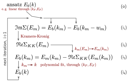
Figure 1: (Color online) Self-consistent iterative algorithm that refines the bare band $E_{b}$ by enforcing the Kramers-Kronig relation between $\mathfrak{Im}\Sigma$ and $\mathfrak{Re}\Sigma$.

In this work we propose a simpler procedure, that avoids the need for a minimization of a functional, and achieves the self-consistency in just a few iterations. The procedure also appears to be more stable with respect to the noise present in the experimental data, and no denoising(Norman et al., 1999) or smoothing by fitting to a function (Bianchi et al., 2010) is needed.

The algorithm, shown in Fig. 1, starts by postulating a form, linear for example, of the bare band $E_{b}(k)$. Forcing the function to pass through the experimentally determined point ($k_{F}$, $E_{F}$) can help in faster convergence. Note that this constraint is physically sound, as the renormalized and the bare-band are expected to intersect at the Fermi level. In the first step of the iterative procedure, $\mathfrak{Im}\Sigma$ is calculated by eq. (3). In the second step $\mathfrak{Re}\Sigma$ is obtained by a discrete Hilbert transform of $\mathfrak{Im}\Sigma$. This is then by eq. (2) used to refine the bare band, first on a discrete set of points (step 3), then fitted to a polynomial or a function at wish (step 4). The iteration ends when there are no substantial changes in the functions (or parameters) obtained. Further details on the procedure, the full code and exemplary input data are accessible as supplemental material in Ref. Sup, .

Electron-phonon coupling strength can be extracted (Fink et al., 2006) either from a steplike increase of the imaginary part of the self-energy, $\Delta\mathfrak{Im}\Sigma$, as

$$\lambda=\frac{2}{\pi}\frac{\Delta\mathfrak{Im}\Sigma}{\hbar\omega_{ph}}$$ (6)

or from the real part of the self energy, as

$$\lambda=-\frac{\mathrm{d}}{\mathrm{d}E}\mathfrak{Re}\Sigma(E)|_{E=E_{F}}$$ (7)

Although these two equations are strictly valid only at zero temperature, they are especially good approximation in the case of graphene, where phonon excitations are high in energy.

Instead of calculating the derivative in eq. (7) directly, which is liable to errors due to the noise and scarcity of reliable data in the very proximity of the Fermi level, one can make use of eq. (2), through $\lambda=-\frac{\mathrm{d}}{\mathrm{d}E_{m}}(E_{m}-E_{b}(k_{m}))=\frac{E_{b}^{\prime}(k)}{E_{m}^{\prime}(k)}-1$, to get

$$\lambda=\frac{v_{b}(E_{F})}{v_{r}(E_{F})}-1$$ (8)

Here, $v_{b}$ ($v_{r}$) is the Fermi velocity of the bare (renormalized) band.

III Experimental

The experiments were performed at the APE beamline at ELETTRA. Iridium single crystal of 99.99% purity and surface orientation better than 0.1° was used. The substrate was cleaned by several cycles of sputtering with 1.5 keV Ar⁺ ions at room temperature followed by annealing at 1600 K. Cleanness and quality of Ir(111) were checked by ARPES (existence and quality of iridium surface states)(Pletikosić et al., 2010) and low energy electron diffraction (LEED). The base pressure was 5·10^–9 Pa.

During the growth of graphene the surface was exposed to 2 Langmuir (L, 1L=1.3·10^–4 Pa·s) of ethene at 300 K and subsequently heated to 1470 K. In order to ensure perfectly oriented graphene and the coverage of the whole surface, the procedure was repeated up to 12 times, finishing with simultaneous exposure to ethene and heating. (Kralj et al., 2011; Hattab et al., 2011) Potassium was added at room temperature by evaporation from a getter source, until a clear 2×2 structure emerged in LEED and no additional doping of graphene bands could be achieved.

ARPES spectra have been collected by a Scienta SES 2002 analyzer. For this experiment we used photon energy of 40.5 eV, in s and p polarization of the field. Typical spot size on the sample was 50×100 $\mathrm{\mu m}$. The energy resolution of this setup was about 12 meV, and the angular resolution 0.1°. The azimuths were checked according to the orientation of spots in LEED and the emergence of the Dirac cone and replica bands in ARPES for the plain graphene on Ir(111). (Pletikosić et al., 2009) During the measurements the temperature of the sample was held at 80 K.

IV Results

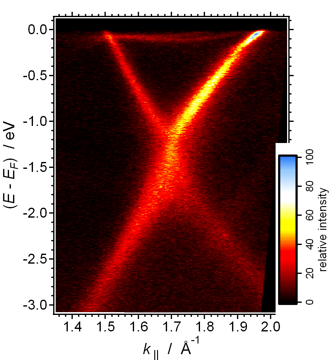
Figure 2: (Color online) ARPES spectrum (excitation energy 40.5 eV, $s$ polarization, scan direction $\Gamma$-K-M) showing the intensity of photoemission from the Dirac cone in graphene/Ir(111) saturated with potassium.

Figure 2 shows photoemission spectrum of potassium-intercalated graphene on Ir(111) around the K point along the $\Gamma$-K-M direction. The spectrum shows a discernible asymmetry of the intensity, such that the part of the spectrum of the $\pi^{*}$ band along K-M ($k>1.7$ Å^-1) exhibits much stronger intensity than the part dispersing along K-$\Gamma$ ($k<1.7$ Å^-1). Notice that iridium surface state at the Fermi level, also present in the spectrum for graphene/Ir(111), (Pletikosić et al., 2009) is not quenched by the intercalation of potassium. Potassium doping, however, has rather strong effect on the $\pi$ bands of graphene — shifts the Dirac point to higher binding energies and renormalizes the band dispersion just below the Fermi level.

The position of the Dirac point, being defined as a single point in momentum space where the $\pi$ bands cross each other, is not straightforward to determine. As can be seen from Fig. 2 there is no such well-defined crossing point here. This is presumably due to a band gap, as a study by Varykhalov et al. (2010) has shown that some metallic dopands do induce a band gap at the Dirac point. We estimate the width of the band gap to be 0.3 eV with the position of the Dirac point at 1.35 eV below the Fermi level, which is, within a tenth of an eV, equal to the values previously obtained for graphene/Ir(111) (Bianchi et al., 2010) and some other systems, such as graphene/SiC (Grüneis et al., 2009) and graphite(Valla et al., 2009).

The shift of the Dirac point to higher binding energies causes an increase of the Fermi surface, which is for higher doping levels characterized by trigonal warping; i. e. an effect when a transformation of the constant energy maps from circular to trigonal shape takes place. (Grüneis et al., 2009; McChesney et al., 2010) The trigonal warping is clearly associated with different values of $k_{F}$ for the $\pi^{*}$ band dispersing from K to M or $\Gamma$. We have determined $k_{F}$ along the directions K-$\Gamma$ and K-M to be 0.18 Å^-1 and 0.27 Å^-1 respectively, and used these values to estimate the doping level of about 0.05 electrons per unit cell.

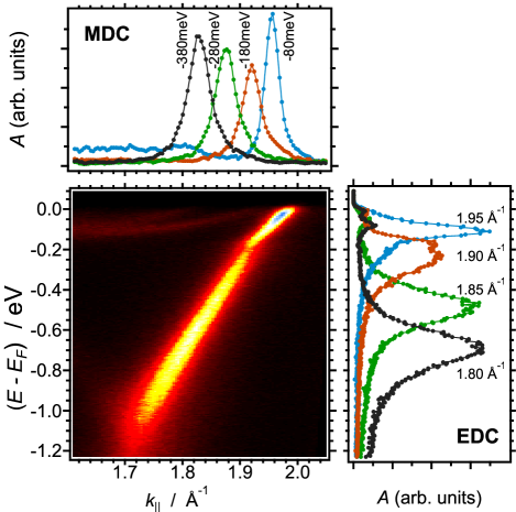
Figure 3: (Color online) ARPES spectrum of potassium intercalated graphene/Ir(111) (excitation energy 40.5 eV, p polarization, scan direction $\Gamma$-K-M) along with a few selected MDC and EDC cuts at given energies and momenta.

A prominent feature of the spectrum in Fig. 2 is the renormalization of the K-M branch of the $\pi^{*}$ band just below the Fermi level. No such renormalization is as obvious for the branch K-$\Gamma$. This kink-like change of the band dispersion is detailed in Fig. 3.

As we have pointed out, two parts of the spectrum in Fig. 2 show a considerable difference of spectral intensity. The change of the light polarization can additionally alter this intensity ratio. We used p polarization of the incident light in order to extinguish spectral features along K-$\Gamma$ entirely, leaving only the part of the $\pi^{*}$ band along the K-M direction visible. The origin of the diminishing spectral intensity has been explained by Gierz et al. (2011) The change of the light polarization strongly enhances signal to noise ratio which shows to be essential in detailed spectrum analysis, as will be demonstrated in the following. Simple inspection of Fig. 3 places the phonon induced dispersion kink at around 200 meV below the Fermi level. Notice how the dispersion kink is now even more pronounced, accompanied by a strong drop of the spectral intensity at the kink. In the following we present a detailed analysis of the spectrum along the K-M direction, and only state the results for the K-$\Gamma$ direction for which the analysis is presented in the supplemental material, Ref. Sup, .

V Analysis and discussion

A set of MDC and EDC cuts in Fig. 3 illustrates the kind of analysis made for each and every slice of the ARPES spectrum shown. MDCs are generally characterized by a continuous change of the peak position without any substantial change of the lineshape, apart for the width of the peaks. However, in the narrow region around the kink, the EDCs clearly exhibit double peak structure, that can be fitted with two Lorentzians. The energy splitting between the peaks is found to be around 60 meV. Farther away, ±70 meV from the kink, EDCs can be described by a single Lorentzian. A small peak visible in EDCs just below the Fermi level is associated with the S₁ surface state of Ir(111). (Pletikosić et al., 2010)

Note that the full width at half maximum of the MDC at an energy just below the Fermi level (Fig. 2) is 0.022 Å^-1, which is even slightly smaller than the width measured for bare graphene on Ir(111) (Kralj et al., 2011) and comparable to non-intercalated graphene on SiC (Bostwick et al., 2007). The measured width of 0.022 Å^-1 is substantially smaller than the previously reported value of 0.095 Å^-1 for the same system. (Bianchi et al., 2010) This questions the conclusion by Bianchi et al. (2010) that the doping of graphene/Ir(111) by potassium increases the electron scattering rate due to the loss of translation symmetry induced by the incommensurability of graphene and Ir(111). Our data imply that the intercalation of potassium, observed as a disappearance of graphene’s moiré superstructure, does not increase the electron scattering rate compared to bare graphene on Ir(111). Therefore, we can conclude that potassium intercalated into graphene/Ir(111) system does not act as an additional scattering center. As we shall demonstrate later, the measured value of the MDC width translates into rather big quasiparticle scattering time. The MDC width increase (to 0.042 Å^-1) measured below the dispersion kink (Fig. 2) fits into the picture of phonon-induced renormalization of the $\pi^{*}$ band.

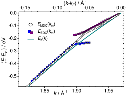
Figure 4: (Color online) Peak positions extracted from MDC cuts (circles) and EDC cuts (squares) of the spectrum shown in Fig. 3. Thick line shows the bare-band $E_{b}(k)$ obtained from the self-consistent procedure.

Figure 4 summarizes the peak positions obtained from MDC and EDC sets of spectra from Fig. 3. Open circles represent peak positions obtained from the analysis of MDCs, while squares are obtained from EDCs. The fact that the two dispersions do not coincide, especially in the region above the kink is easy to understand when one takes into account that the spectral intensity of the band sharply changes, and that what is a local maximum $k_{m}$ in a horizontal cut along $E=E_{m}$ does not have to be a local maximum in a vertical cut along $k=k_{m}$. The data below and above the kink are fitted with two linear functions with noticeably different slopes. The data far away from the Fermi level can be fitted with a linear curve and the corresponding band velocity equals to $0.7\cdot 10^{6}$ m/s. This represents a reduction of about 30% compared to the $\pi$ band of nearly neutral graphene on Ir(111), and is consistent with the predicted reduction of the Fermi velocity, as calculated by Park et al. (2009) The set of MDC data between the Fermi level and the kink is also fitted with a linear function defined by the band velocity (which is in this case the Fermi velocity as well) $v_{r}(E_{F})=0.46\cdot 10^{6}$ m/s. Note that this value is only about half the Fermi velocity of the $\pi$ band in bare graphene on Ir(111) (Kralj et al., 2011) and the $\pi^{*}$ band on SiC (Siegel et al., 2011a). This renormalization of the velocity can lead to an overestimate of the coupling strength to phonons for the simple reason that the change of the electron velocity near $E_{F}$ is largely due to the curvature of the $\pi^{*}$ band induced by other interactions and only to small extent by electron-phonon coupling. (Park et al., 2008b)

In order to take into account the nonlinearity of the $\pi^{*}$ band, the bare-band function $E_{b}(k)$ was self-consistently reconstructed from the MDC data, by the recursive procedure described above. The $\pi^{*}$ band itself has been measured far below the phonon-induced kink, where the contribution to $\mathfrak{Re}\Sigma$ can be neglected and the bare-band approaches the measured. (Kordyuk et al., 2005) This gives confidence to the functions obtained, as the problem of tails is greatly avoided. The corrections of $E_{m}(k)$ leading to $E_{b}(k)$ being mostly due to low-energy phonon excitations, the function $E_{b}(k)$ can be considered as one that takes into account all electron interactions except those with phonons.

The derivative of the bare function at the Fermi level gives the Fermi velocity for the bare band $v_{b}(E_{F})=0.56\cdot 10^{6}$ m/s. The obtained values of band velocities, at the Fermi level and far away from the kink, are in very good agreement with the values of the band velocities for highly doped graphene, reported by Siegel et al. (2011a)

To summarize, it is clear that a large portion of the velocity reduction as we approach the Fermi level comes from the non-linear nature of the bare $\pi^{*}$ band. The modification of the Fermi velocity due to the coupling to phonons is accordingly rather small, around 0.1·10⁶ m/s, which is only a 10% change.

The ratio between the Fermi velocity of the bare band and the electron-phonon-induced renormalized velocity at the same energy gives, by eq. (8), the value of the electron-phonon coupling strength. Accordingly, the value of $\lambda$ along the K-M direction equals to 0.22. The same analysis on the K-$\Gamma$ direction gives $\lambda=0.19$. (Sup, ) Previously, Bianchi et al. (2010) obtained $\lambda=0.28$ for both directions.

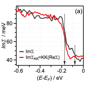
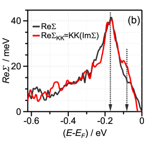
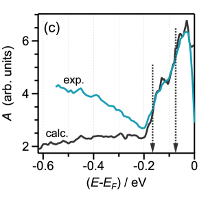
Figure 5: (Color online) A set of self-consistent functions obtained from MDC cuts of the spectrum shown in Fig. 3 and the bare-band shown in Fig. 4. (a) black line: $\mathfrak{Im}\Sigma$ calculated by eq. (3); red line: $\mathfrak{Im}\Sigma_{KK}$ as a Kramers-Kronig transform of $\mathfrak{Re}\Sigma$; (b) black line: $\mathfrak{Re}\Sigma$ calculated by eq. (2); red line: $\mathfrak{Re}\Sigma_{KK}$ as a Kramers-Kronig transform of $\mathfrak{Im}\Sigma$. (c) spectral intensity $A(E)$ from the experiment (blue line) and calculated from the self-consistent data by eq. (1) (black line). Arrows indicate the energies of phonons that induce band renormalization.

We use MDCs extracted from the spectrum shown in Fig. 3 to plot (a) imaginary part of the self-energy, $\mathfrak{Im}\Sigma(E)$ (b) real part of the self-energy, $\mathfrak{Re}\Sigma(E)$ and (c) spectral intensity of the MDC peaks, $A(E)$. Figure 5 shows the results. The functions plotted in black were calculated from formulæ (1)–(3) using the bare-band from our self-consistent iterative procedure. The functions shown in red illustrate the degree of self-consistency achieved; the one for $\mathfrak{Im}\Sigma_{\mathrm{KK}}$ in Fig. 5(a) was obtained by Kramers-Kronig transformation of the data for $\mathfrak{Re}\Sigma$ from Fig. 5(b), and equally, the one for $\mathfrak{Re}\Sigma_{\mathrm{KK}}$ from the data for $\mathfrak{Im}\Sigma$. The overall agreement is quite good. We find the data for FWHM and consequently for $\mathfrak{Im}\Sigma$ more reliable, the noise being pretty low and the relative error being smaller in determining the width of the MDCs than the peak positions, from which $\mathfrak{Re}\Sigma$ is calculated. The effects of experimental smearing also have a greater impact on the fine details of MDC peak positions, adding only a constant background to FWHMs and $\mathfrak{Im}\Sigma$. We suspect that the low-energy shoulder in $\mathfrak{Re}\Sigma$ (and the associated step in $\mathfrak{Im}\Sigma_{KK}$) are for these reasons less pronounced than the corresponding ones in $\mathfrak{Re}\Sigma_{KK}$ (and $\mathfrak{Im}\Sigma$). The difference in experimental and calculated spectral intensities in Fig. 5(c) at the high-energy side probably comes from the fact that the calculated renormalized band $E_{b}(k_{m})+\mathfrak{Re}\Sigma(E_{m})$ does not come close enough to the measured band $E_{m}(k_{m})$, as the increase of the spectral function would come from one approaching the other (see Eq. 1). We suspect this could be a still-observable consequence of the missing high-energy tails. (Kordyuk et al., 2005)

Generally, a step-like increase of $\mathfrak{Im}\Sigma(E)$ and a maximum of $\mathfrak{Re}\Sigma(E)$ at the same energy is associated with electron coupling to some excitation, in this case phonons. As pointed out by McChesney et al. (2008) the coupling to a phonon should have a profound impact on the energy dependence of the spectral intensity $A(E)$ as well.

Instead of one, all displayed spectral parameters show consistently two features that can be accordingly associated with the coupling to two phonons, one at 170 meV and the second one at 75 meV. Arrows in Figs. 5 (a)–(c) indicate the energies of these two phonons.

The $\mathfrak{Im}\Sigma(E)$ (Fig. 5a) shows a distinct step-like increase between 0.05 and 0.1 eV below the Fermi level with the initial value of 39 meV which reaches a local maximum of 52 meV at 0.1 eV. This increase of $\mathfrak{Im}\Sigma(E)$ is associated with the phonon of energy 75 meV. Further increase of $\mathfrak{Im}\Sigma(E)$ up to 85 meV induced by the coupling to a phonon of 170 meV takes place between 0.13 and 0.21 eV. Below that, $\mathfrak{Im}\Sigma(E)$ stays constant up to 0.4 eV, but then starts to increase with energy, due to other contributions to the lifetime (electron-electron, electron-plasmon). (Bostwick et al., 2007)

Electron-phonon coupling constant can be extracted from the change of $\mathfrak{Im}\Sigma(E)$ by eq. (6). (Fink et al., 2006; Grüneis et al., 2009) The total increase of $\mathfrak{Im}\Sigma(E)$ equal to 46 meV, translates to $\lambda=0.17\pm 0.01$ along the K-M direction. A similar analysis of $\mathfrak{Im}\Sigma(E)$ along the K-$\Gamma$ direction gives $\lambda=0.18\pm 0.02$. (Sup, )

$\mathfrak{Re}\Sigma(E)$, consistently with $\mathfrak{Im}\Sigma(E)$ and $A(E)$, shows a peak at 170 meV and a distinct shoulder at a lower binding-energy side, which clearly implies an existence of two excitations that contribute to the renormalization of the bare band dispersion.

Using the imaginary part of the self-energy in the proximity of the Fermi level, we determine the photohole scattering time, $\tau=\frac{\hbar}{2\,\mathfrak{Im}\Sigma}$, (Calandra and Mauri, 2007) to be bigger than 10 fs. This is the same value as obtained for high quality graphene on SiC. (Sprinkle et al., 2009) Note that this value is not to be compared to the scattering time in mobility measurements ($\sim 350$ fs), as those include some more scattering mechanisms. (Calandra and Mauri, 2007)

As pointed out, the energy dependence of the spectral intensity $A(E)$ also indicates the existence of two distinct phonon excitations that couple to electrons. McChesney et al. (2008) have demonstrated a high sensitivity of $A(E)$ to many-body interactions, drawing attention to the fact $A(E)$ can access even a faint contributions to the self-energy with a sensitivity even better than $\mathfrak{Im}\Sigma(E)$ can provide. In agreement with this model we observe two shoulders in $A(E)$ where an onset of each shoulder corresponds to a phonon excitation (see Fig. 2 in Ref. McChesney et al., 2008). Summarizing the features that have been observed in three parameters: $\mathfrak{Im}\Sigma(E)$, $\mathfrak{Re}\Sigma(E)$ and $A(E)$, we can conclude, with a high degree of consistency, that the phonon energies that induce the renormalization of the dispersion of the $\pi^{*}$ band of doped graphene along the K-M direction have energies equal to 170 meV and 75 meV. These two phonons can be associated with an optical phonon (transverse or longitudinal) around K and an acoustic phonon, respectively. According to González and Perfetto (2009), in non-interacting graphene these phonons should be in-plane oscillations as the symmetry does not allow coupling of the out of plane phonons to electrons in graphene. However the presence of the substrate might break the 2D symmetry of graphene and hence allow the coupling of both in-plane and out-of-plane oscillations to electrons in graphene.

Some theoretical calculations also support the notion of a two-phonon-spectrum that induces renormalization of graphene bands close to the Fermi level. According to Calandra and Mauri (2007), the $\pi^{*}$ band of doped graphene should show two kinks in the dispersion (accordingly accompanied by two steps in the MDC linewidth), one at 195 meV being attributed to A₁ mode and another at 160 meV which corresponds to a twofold degenerate E_2g mode. Previous measurements of Bianchi et al. (2010) with graphene on Ir(111) showed signatures in the band dispersion and widths of spectral curves of apparently only one phonon. However, their self-consistent analysis showed that the experimental data can be modelled by contributions of five Einstein oscillators with energies that are evenly distributed over the range from 21 meV to 190 meV.

Interestingly, the pattern of coupling similar to the one we observed in graphene/Ir(111) is also reported for CaC₆ where the contributions to the self-energy come from two phonons, one at 75 meV and the other at around 160 meV. (Valla et al., 2009) This agreement supports the notion that intercalated atoms (K or Ca) do not participate in the coupling of the $\pi^{*}$ band to phonon modes apart from the doping effect.

The energy splitting between the EDC peaks has already been observed in materials with strongly coupled electrons and phonons. (Hengsberger et al., 1999; LaShell et al., 2000) Although the coupling in graphene is not as large, its two-dimensionality is, according to Badalyan and Peeters (2012), a possible reason for an enhancement of the effective coupling in the vicinity of the phonon energy. An electron-phonon complex quasiparticle forms, giving rise to a strong modification of the Dirac spectrum, seen as the branches of the $\pi^{*}$ band in the neighborhood of the phonon emission threshold.

The value of the electron-phonon coupling constant obtained in this work ($\sim 0.2)$ is somewhat smaller than the one obtained by Bianchi et al. (2010) for the same system ($\sim 0.3)$. Nevertheless, the value derived from our spectra does not support the notion of Siegel et al. (2011b) that the coupling in n-doped graphene on a metallic surface should be still a few times smaller ($\sim 0.04$). Given sharp enough spectra, low in background intensity and noise, a pronounced kink in the $\pi^{*}$ band dispersion, and especially a steplike increase of the spectral width at the phonon energy, must alone be a clear sign of a non-negligible strength of interaction, whatever the choice for the bare band is.

VI Conclusions

In conclusion, we have analyzed various parameters from high resolution ARPES measurements — peak positions and widths of MDCs, imaginary and real part of the self-energy $\Sigma(E)$, spectral intensity $A(E)$ — all consistent with the notion that two phonons contribute to the renormalization of the band dispersion in graphene on Ir(111): a high energy phonon at 170 meV and a low energy phonon at 75 meV. The coupling constant associated with these two phonons is around 0.2, which is similar to a previous finding for the same system. We have also found that the intercalation of potassium up to saturation does not increase the scattering rate of the photohole in the $\pi^{*}$ band. Due to the perfectness of the K/graphene/Ir(111) structure the quasiparticle (photohole) scattering time can be posed exceptionally high, above 10 fs.

Finding the bare band: Electron coupling to two phonon modes in potassium-doped graphene on Ir(111)

I. Pletikosić, M. Kralj, M. Milun, P. Pervan

Supplemental Material

Formulæ

Under the assumption that the self-energy does not depend on momentum, equations (2) and (3) from our article are exact whatever the bare-band function $E_{b}(k)$ is. However, in order to use the linearized version of eq. (3) — $\mathfrak{Im}\Sigma(E_{m})=\hbar v_{b}(E_{m})\cdot w_{m}$, where $v_{b}(E_{m})=\frac{1}{\hbar}\frac{d}{dk}E_{b}(k)|_{k=k_{m}(E_{m})}$ — the measured band should be sufficiently sharp ($w_{m}$ sufficiently small), and the bare band piecewise linear (giving a symmetric peak, $w_{L\,m}=w_{R\,m}=w_{m}$). Even in our case of very narrow MDC peaks (0.010 Å^-1<$w_{m}$<0.022 Å^-1, or 0.007 Å^-1<$w_{m}$<0.018 Å^-1 when the experimental resolution is deconvolved) this is only partially fulfilled. The figure below illustrates the relations for $\mathfrak{Im}\Sigma$, $\mathfrak{Re}\Sigma$ and $E_{b}$ in the case of real experimental data on $E_{m}(k_{m})$ and FWHM ($2\,w_{m}$). Also shown is an MDC curve for $E_{m}=-0.13$ eV with FWHM of 0.026 Å^-1.

In the following, we shall not use the linearized version of eq. (3), in spite of rather narrow peaks, and only make use of $w_{L\,m}=w_{R\,m}=w_{m}$, as our Lorentzians are quite symmetric.

Method

Instead of finding $E_{b}(k)$ by cleverly trying the parameters that define the function in a method commonly used before (Method I on the right), using Levenberg–Marquardt algorithm, for example, the idea is to employ a loop algorithm that happens to be self-correcting and relatively easy to implement (Method II on the right).

Here, $\mathfrak{Re}\Sigma(E_{m})$ obtained from the Kramers-Kronig transform of $\mathfrak{Im}\Sigma$ is used to calculate $E_{b}$ from the measured renormalized dispersion $E_{m}(k_{m})$ on a discrete set of points. Then, by least-squares fitting, a functional form $E_{b}(k)$ is acquired, and used to calculate $\mathfrak{Im}\Sigma$ in the next iteration.

METHOD I

METHOD II

Convergence

The figure below shows the convergence of the bare-band function. The iteration starts by postulating a linear band (i_o). Already the second iteration (i₂) gives the band indistinguishable from those obtained in the following iterations. Also shown is how the coefficients of a third-order polynomial for $E_{b}$

$$E_{b}(k)=0+c_{1}k+c_{2}k^{2}+c_{3}k^{3}$$

converge oscillatory through the course of iterations.

Notice that the renormalized and the bare-band merge quite close to the kink, giving confidence that the influence of the missing tail is negligible.

Code

Two procedures to be used in Wavemetrics IgorPro data analysis software are presented. The first procedure, scKK_setup, is used for initialization, with properly scaled one-dimensional waves containing data on the positions (km) and widths (fwhm) of MDC Lorentzian curves; examples are given in the next section. The second procedure, scKK_iteration, is called for several times, until the convergence in the output waves (scEb, scEb_fit, scImS, scReS…) is achieved.

We find it convenient to put ($k_{F}$,$E_{F}$)=(0,0), as that point can be read-off the spectrum with high enough accuracy, and make the bare-band function pass through it.

Instead of a polynomial, any fitting function (e.g. a tight-binding formula) should be easy to implement. As we are usually not interested in $E_{b}$, but in the results obtained for $\mathfrak{Im}\Sigma$ and $\mathfrak{Re}\Sigma$, polynomial fitting is sufficient.

⬇ // // Author: Ivo Pletikosic, ivo.pletikosic@ifs.hr, November 2011 // // sc = self-consistent; KK=Kramers-Kronig // first, create waves needed for the iteration procedure // wave km(Em) contains the experimental dispersion, i.e. maxima of the spectral function // wave fwhm(Em) contains widths of Lorentzian peaks at a given energy // x axes should be properly scaled! // energy is measured from the Fermi level, (E-EF) Function scKK_setup(km,fwhm) Wave km,fwhm // (km-kF) as a function of Em Duplicate/O km,scKKm // putting the origin of the k axis to kF (a point where Em=0) Variable kF=km(0); scKKm=km-kF Duplicate/O fwhm,hwhm; hwhm*=0.5 // sample ReS at the same energies as KKm Duplicate/O scKKm,scReS // sample ImS at the same energies as hwhm Duplicate/O hwhm,scImS // discrete bare band Eb; Em(km); and an auxiliary wave Make/O/N=(numpnts(scKKm)) scEb,scEm,Em_scaling // scaling from the first/last k-point of the experimental dispersion SetScale/I x,scKKm[0],scKKm[numpnts(scKKm)], "A\S-1\M",scEb, scEm SetScale y,0,0,"eV",scEb,scEm // this will be used in the interpolation to get Em(km) from km(Em) SetScale/I x,leftx(scKKm),leftx(scKKm)+deltax(scKKm)*(numpnts(scKKm)-1),Em_scaling Em_scaling=x // Em as a function of (km-kF) scEm=interp(x,scKKm,Em_scaling) // zeroth approximation to Eb: // a line through (kF,EF)=(0,0) and the lowest point of the experim. dispersion Make/O cw={0,leftx(scKKm)/scKKm[0]} scEb=poly(cw,x) // this will become symmetrized and resampled ImS Make/O/N=(4*numpnts(scImS)) symmImS SetScale/I x,leftx(scImS),-leftx(scImS),"eV",symmImS // this will become symmetrized and resampled ReS Make/O/N=(4*numpnts(scReS)) symmReS SetScale/I x,leftx(scReS),-leftx(scReS),"eV",symmReS End

⬇ // iteration function // call it several times until there’s no substantial change in the output waves // polyN is the degree of the band fitting polynomial [2, 3, ..., 7] Function scKK_iteration(polyN) Variable polyN Wave scKKm, scEb, scReS, scImS Wave Em, hwhm, cw, symmReS, symmImS // some auxiliary waves PauseUpdate; // start from ImS scImS=poly(cw,scKKm(x)) - poly(cw,scKKm(x)-hwhm(x)) // or //scImS=poly(cw,scKKm(x)+hwhm(x)) - poly(cw,scKKm(x)) // or //scImS=0.5*(poly(cw,scKKm(x)+hwhm(x)) - poly(cw,scKKm(x)-hwhm(x))) // K-K transform ImS to HReS // symmetrize symmImS=(x<=0) ? scImS(x) : scImS(-x) // ReS from the K-K transform of ImS HilbertTransform/DEST=scHReS symmImS scHReS*=-1 SetScale/P x,leftx(symmImS),deltax(symmImS),"eV",scHReS // ansatz for Eb in the next iteration // bare band as a function of km (therefore, of all the discrete k’s present in the spectrum) scEb=Em(x)-scHReS(Em(x)) // fit Eb to a polynomial (could be any other function), as we’ll need some extrapolation // initial values of the fitting polynomial coefficients: all 0 Make/O/N=(polyN+1) cw=0 // keep c0=0, i.e. make the polynomial zero at (kF,EF)=(0,0) String fmtStr; sprintf fmtStr,"1%0*.0f" polyN, 0; // functional (i.e. smooth) form of the bare band Duplicate/O scEb,scEb_fit // the output of this cmd will be used for the next iteration CurveFit/Q/H=fmtstr/NTHR=1 poly (polyN+1), kwCWave=cw, scEb /D=scEb_fit // print fitting coefficients print cw // and just to check things out // ReS from the very definition // poly(...) represents a smooth function for Eb from the previous iteration scReS=x - poly(cw,scKKm(x)) // antisymmetrize symmReS=(x<=0) ? scReS(x) : (-scReS(-x)) // ImS from the K-K transform of ReS HilbertTransform/DEST=scHImS symmReS SetScale/P x,leftx(symmReS),deltax(symmReS),"eV",scHImS // offset, as HilbertTransform seems to make mean=0 scHImS+=mean(scImS) End

Data

Examples of input waves for the self-consistent iterative procedure, as extracted from MDCs of an ARPES spectrum analyzed in our paper.

IgorPro file km.itx

(here downsampled to $\Delta=0.012$ eV from the original $\Delta=0.005$ eV)

⬇ IGOR WAVES km BEGIN 1.797 1.799 1.801 1.804 1.806 1.809 1.812 1.814 1.817 1.819 1.822 1.824 1.827 1.830 1.834 1.836 1.838 1.841 1.844 1.846 1.849 1.852 1.854 1.857 1.859 1.862 1.864 1.867 1.870 1.872 1.875 1.878 1.880 1.883 1.886 1.889 1.891 1.893 1.895 1.898 1.900 1.903 1.905 1.907 1.910 1.913 1.918 1.922 1.927 1.932 1.936 1.940 1.944 1.947 1.951 1.955 1.959 1.963 1.968 1.971 1.975 END X SetScale/P x -0.7,0.012,"eV", km X SetScale y 0,0,"1/A", km  

IgorPro file fwhm.itx

(here downsampled to $\Delta=0.012$ eV from the original $\Delta=0.005$ eV)

⬇ IGOR WAVES fwhm BEGIN 0.0464 0.0458 0.0453 0.0434 0.0430 0.0445 0.0435 0.0442 0.0423 0.0414 0.0420 0.0407 0.0418 0.0419 0.0415 0.0405 0.0414 0.0420 0.0416 0.0408 0.0398 0.0390 0.0400 0.0405 0.0408 0.0397 0.0398 0.0399 0.0403 0.0405 0.0408 0.0408 0.0413 0.0406 0.0399 0.0419 0.0421 0.0411 0.0415 0.0418 0.0433 0.0436 0.0428 0.0382 0.0361 0.0315 0.0290 0.0282 0.0273 0.0279 0.0278 0.0262 0.0243 0.0233 0.0230 0.0228 0.0224 0.0245 0.0247 0.0246 0.0222 END X SetScale/P x -0.7,0.012,"eV", fwhm X SetScale y 0,0,"1/A", fwhm  

A few questions to answer

• Could the $\mathrm{K}$-$\Gamma$ direction be treated with the same rigor as the K-M direction?

In the experimental geometry we had, the K-$\Gamma$ direction ($k_{||}$<1.7 Å^-1) is not visible in high-intensity spectra recorded with the p polarization of light. This is illustrated in the following two raw images taken with the same excitation energy (40.5 eV) and in the same energy and emission-angle window. One can easily notice a high noise level in the s polarization spectrum where a part of the K-$\Gamma$ direction is seen. The photoemission intensity is about 30 times lower in the s polarization spectrum.

• So, what are the results for the $\mathrm{K}$-$\Gamma$ direction?

We shall analyze the spectrum recorded in the s polarization of the excitation light, shown below. The whole K-$\Gamma$ branch of the doped $\pi^{*}$ band is visible, continuing with a part of the K-M branch. A surface state of Ir(111), touching the renormalized part of the $\pi^{*}$ band is also visible. It influences the analysis of the MDC peak positions and widths in a small range of energies, between -25 meV and -70 meV. These data will have to be interpolated.

We now show the data on FWHM and the position of MDC peaks extracted from the above spectrum, along the K-$\Gamma$ branch of the $\pi^{*}$ band. The widths are comparable to those on the K-M branch, but the noise in the data is obviously larger:

Applying our self-consistent recursive procedure to the data from the K-$\Gamma$ branch, we obtain the bare band (shown above, along with the dispersion of the renormalized band), and the parts of the self energy, $\Sigma=\mathfrak{Re}\Sigma+i\,\mathfrak{Im}\Sigma$:

• Can you simulate a spectral function with the same lambda ($\lambda=0.2$) in the K-M and K-$\Gamma$ direction. It would be interesting to see if the different dispersion in the two directions is responsible for the kink being more obvious in the KM direction.

We simulate this by first recognizing that the same e-ph coupling parameter $\lambda=0.2$ for the phonon of energy $\omega_{ph}=170$ meV means, by equation (6) of our article, the same step in the imaginary part of the self energy. This would be $\Delta\mathfrak{Im}\Sigma=55\,\mathrm{meV}$ for both branches. The real part of the self energy is obtained by the Kramers-Kronig transformation of the imaginary part, assuming particle-hole symmetry:

We then take two linear bare bands, one mimicking the dispersion of the K-$\Gamma$ branch (band velocity $1\cdot 10^{6}$ m/s), the other the dispersion of the K-M branch (band velocity $0.6\cdot 10^{6}$ m/s), and simulate the spectral function by equation (1) from our article:

The renormalized bands can be either extracted from the spectral function following the dispersion of MDC peaks, or calculated by equation (2). This is done self-consistently, starting with $E_{m}^{0}=E_{b}(k)+\mathfrak{Re}\Sigma(E_{b}(k))$ and iterating over $E_{m}^{i+1}=E_{b}(k)+\mathfrak{Re}\Sigma(E_{m}^{i})$. The result can be immediately compared to the experimental data. Even the simple linear band closely follows the measured band in a wide range below the kink, as well as its renormalized part follows the band above the kink. And indeed, the kink is more obvious for the slowly dispersing band, i.e. the band simulating the dispersion along the K-M direction.