Coherent states and related quantizations for unbounded motions

Abstract

We build coherent states (CS) for unbounded motions along two different procedures. In the first one we adapt the Malkin-Manko construction for quadratic Hamiltonians to the motion of a particle in a linear potential. A generalization to arbitrary potentials is discussed. The second one extends to continuous spectrum previous constructions of action-angle coherent states in view of a consistent energy quantization.

I Introduction

At present, coherent states (CS) take an important place in modern quantum mechanics. They have a wide range of applications, in semiclassical description of quantum systems, at the same time in quantization of classical models, in condensed matter physics, in radiation theory, in loop quantum gravity, and so on CSSI12 . In view of this wide range of domains, a universally accepted definition of CS for arbitrary physical systems and a universally accepted construction for them are still lacking. Due to Glauber and Malkin-Manko (see Glauber ; MalMa ) there exists a well-defined construction algorithm for systems with quadratic Hamiltonians (QH) with discrete spectra, and due to Gilmore, Perelomov and others (see gilm72 ; perel72 ; perel86 ; AAG00 ) for systems with a given Lie group symmetry. Approaches based on action-angle formalism gaklau99 or on reproducing kernel combined with Bayesian probabilistic ingredients agh08 ; gazeau09 have been developed more recently. In any generalization, one attempts to maintain some of the basic properties of already known CS for quadratic systems, like resolution of the unity. One of the most popular constraints concerns semi-classical features. One thus attempts to maintain saturation of uncertainty relations for some physical quantities (e.g. coordinates and momenta) as they are given at a certain instant. One requires that means of particle coordinates, calculated with respect to time-dependent CS, move along the corresponding classical trajectories. In addition, CS have to be labeled by parameters that have a direct classical analog, let say by phase-space coordinates. It is also desirable for time-dependent CS to maintain their form under the time evolution. One last but not the least constraint in the construction is to give these special states a status of quantizer à la Berezin-Klauder ber75 ; klau95 ; klau00 ; gazeau09 .

As was already mentioned, usually CS are constructed for systems with discrete energy spectra, which represent bounded motions: we thus pass from quantum stationary states labelled with quantum numbers to quantum CS labelled by phase space variables. There exist some attempts to construct CS for systems with continuous spectra, see for instance hongoh77 ; gaklau99 ; gelklau09 ; GueLoA11 . However, one can state that the problem is still open or at least deserves to be examined in a more comprehensive way, particularly in view of application to realistic systems.

In this article, we examine the problem from two viewpoints. On one side we adopt the approach of Malkin-Manko to systems with continuous spectra. On the other side, we generalize, modify, and apply the approach followed in gaklau99 to the same kind of systems. It should be noted that in the first approach we start with a well-defined quantum formulation (canonical quantization) of the physical system and the construction of coherent states follows from such a quantization. In the second approach, the quantization procedure is inherent to the CS construction itself. In both approaches we pretend to construct CS for concrete systems with continuous spectra, free one-dimensional particle, charged particle on the plane and submitted to an electric field, and eventually one-dimensional particle submitted to an arbitrary scattering potential.

II CS for QH systems with continuous spectra. A possible approach

II.1 An instructive example: a particle in a constant external force

II.1.1 Creation and annihilation operators-integrals of motion

Let us consider the quantum motion of a particle subjected to a constant force that is directed along the axis $x^{1}.$ In fact, it is enough to consider only the one-dimensional motion in the $x^{1}$-direction, since the motions in the $x^{2}$- and $x^{3}$-directions are separated and are free motions. The quantum motion in the $x^{1}$-direction is described by the one-dimensional Schrödinger equation of the form

$$i\hbar\frac{\partial\Psi}{\partial t}=\hat{H}\Psi,\ \ \hat{H}=-\frac{\hbar^{2}\partial_{x^{1}}^{2}}{2m}+\alpha x^{1},$$ (1)

where the constant $\alpha$ determines the magnitude of the force. Introducing dimensionless variables $x$ and$\,\tau$ as

$$x^{1}=lx,\ \tau=\frac{\hbar}{2ml^{2}}t,$$ (2)

where $l$ is an arbitrary constant of the length dimension, Eq. (2) reduces to:

$$i\frac{\partial\Psi}{\partial\tau}=\hat{H}\Psi,\ \ \hat{H}=\sqrt{2}bx-\partial_{x}^{2},\ b=\frac{\sqrt{2}ml^{3}\alpha}{\hbar^{2}}.$$ (3)

Hence we are left with one single dimensionless constant $b$.

We note that the classical trajectory of the position $x$ has the form

$$x\left(\tau\right)=x_{0}+p_{0}\tau-\sqrt{2}b\tau^{2},$$ (4)

where $x_{0}$ and $p_{0}$ are arbitrary constants (initial data).

In spite of the fact that the Hamiltonian $\hat{H}$ has a continuous spectrum, spec $\hat{H}=\mathbb{R},$ it is convenient to introduce in the problem the familiar creation and annihilation operators $a^{{\dagger}}$ and $a$ as follows:

$$a=\frac{x+\partial_{x}}{\sqrt{2}},\ \ a^{{\dagger}}=\frac{x-\partial_{x}}{\sqrt{2}}\Rightarrow$$

$$x=\frac{a+a^{{\dagger}}}{\sqrt{2}},\ \ \partial_{x}=\frac{a-a^{{\dagger}}}{\sqrt{2}};\ \ [a,a^{{\dagger}}]=1.$$ (5)

We recall well-known commutators of such operators which will be useful for the sequel:

$$[a^{{\dagger}}a,a]=[aa^{{\dagger}},a]=-a,$$

$$[a^{{\dagger}}a,a^{{\dagger}}]=[aa^{{\dagger}},a^{{\dagger}}]=a^{{\dagger}},[a^{n},a^{{\dagger}}]=na^{n-1},$$

$$[(a^{{\dagger}})^{n},a]=-n(a^{{\dagger}})^{n-1}.$$ (6)

When written in terms of the operators (5), the Hamiltonian takes the form

$$\hat{H}=\frac{1}{2}(aa^{{\dagger}}+a^{{\dagger}}a-a^{2}-a^{{\dagger}2})+b(a+a^{{\dagger}}).$$ (7)

The term $a^{2}-a^{{\dagger}2}$ impedes the Hamiltonian to be reduced to an oscillator-like form through a canonical transformation, which indicates that there does not exist a ground state and the spectrum of $\hat{H}$ is continuous.

For the oscillator-like quadratic Hamiltonians, CS are constructed with the aid of a Fock discrete basis issued from the action of the creation operators on the vacuum state $|0\rangle$ ($a|0\rangle=0$). Then the Glauber-type instantaneous CS have the form $|z\rangle=D\left(z\right)|0\rangle,$ where the unitary operator $D\left(z\right)$ reads

$$D\left(z,a,a^{{\dagger}}\right)=\exp\left\{za^{{\dagger}}+z^{\ast}a\right\}.$$

In the course of the evolution the CS maintain their form with some time dependent $z\left(t\right).$ The Malkin-Manko-type CS can be defined as eigenvectors of some annihilation operators that are integrals of motion, see MalMa . In fact both constructions coincide for quadratic Hamiltonians. In the case under consideration, it does not exist a generalization of the Glauber construction, because of the absence of the vacuum vector. However, the Malkin-Manko idea can be implemented, as we describe below.

Let us construct an operator

$$\hat{A}\left(\tau\right)=f(\tau)a+g(\tau)a^{{\dagger}}+\varphi(\tau),$$ (8)

where the functions $f(\tau),\,g(\tau)$, and$\,\varphi(\tau)$ have to be determined by demanding that the operator $\hat{A}\left(\tau\right)$ be integral of motion of the equation (3). To this end operator $\hat{A}$ has to obey the condition

$$[\hat{S},\hat{A}\left(\tau\right)]=0,\ \ \hat{S}=i\frac{\partial}{\partial\tau}-\hat{H}.$$ (9)

Using relations (6), one can see that the conditions (9) holds if the functions $f(\tau),\,g(\tau),\,\varphi(\tau)$ are solutions to the system

$$i\dot{f}+f+g=0,\ \ i\dot{g}-f-g=0,\ \ i\dot{\varphi}+b(f-g)=0.$$ (10)

The general solution of eqs. (10) has the form

$$f(\tau)=c_{1}+i(c_{1}+c_{2})\tau,\ \ g(\tau)=c_{2}-i(c_{1}+c_{2})\tau,$$

$$\varphi(\tau)=b\tau[i(c_{1}-c_{2})-(c_{1}+c_{2})\tau]+c_{3}$$

$$\ =b\tau\left\{\left[f(\tau)+g(\tau)\right]\tau+i\left[f(\tau)-g(\tau)\right]\right\}+c_{3},$$ (11)

where $c_{j},\ j=1,\,2,\,3,$ are arbitrary complex constants. Without loss of generality, we can set $c_{3}=0$.

We note that there is no nontrivial solution to (10) that satisfies the condition $f(\tau)=g(\tau)$.

It follows from Eqs. (5) and (8) that

$$[\hat{A}\left(\tau\right),\hat{A}^{{\dagger}}\left(\tau\right)]=\Delta=|f(\tau)|^{2}-|g(\tau)|^{2}=|c_{1}|^{2}-|c_{2}|^{2}.$$ (12)

If $\Delta>0$, then, without loss of generality, we can set $\Delta=1,$ which corresponds to the multiplication of $\hat{A}$ by a complex number. In this case the operators $\hat{A}^{{\dagger}}\left(\tau\right)$ and $\hat{A}\left(\tau\right)$ are familiar creation and annihilation operators.

If $\Delta=0$, then, without loss of generality, the operator $\hat{A}\left(\tau\right)$ can be considered as a self-adjoint one. ($\hat{A}\left(\tau\right)$ can differ from a self-adjoint one only by a complex factor only). In this case, Eqs. (11) contain only one complex constant $c$ and have the form

$$f(\tau)=c+i(c+c^{\ast})\tau,\ \ g(\tau)=f^{\ast}(\tau),$$

$$\varphi(\tau)=b[i(c-c^{\ast})\tau-(c+c^{\ast})\tau^{2}],\ \ \varphi(\tau)=\varphi^{\ast}(\tau).$$ (13)

Finally, if $\Delta<0$, then one has to treat $\hat{B}=\hat{A}^{{\dagger}}$ as an annihilation operator and we again have the case $\Delta>0$. Therefore, in fact, we have to study only two cases: $\Delta=1,\,\Delta=0$.

II.1.2 Coherent states

Let us consider solutions $\psi(\tau;x)$ of the equation (3) that, at the same time, are eigenstates of the operator $\hat{A}\left(\tau\right),$ with the eigenvalues $Z,$

$$\hat{A}\left(\tau\right)\psi(\tau;x)=Z\psi(\tau;x).$$ (14)

Let us consider the case $\Delta=1$. Here, we have a family of operators $\hat{A}\left(\tau\right)=\hat{A}\left(\tau,c_{1},c_{2}\right)$ parametrized by complex numbers $c_{1}$ and $c_{2}$ such that $|c_{1}|^{2}-|c_{2}|^{2}=1.$ One can see that the spectrum of any $\hat{A}\left(\tau\right)$ is continuous, spec $\hat{A}\left(\tau\right)=\mathbb{C},$ and the eigenstate $\psi_{Z}^{c_{1},c_{2}}(\tau;x)$ corresponding to $Z$ can be constructed in two ways.

The states $\psi_{Z}^{c_{1},c_{2}}(\tau;x)$ can be simply found as solutions of the differential equation (14), taking the operator $\hat{A}\left(\tau\right)$ in the coordinate representation (8) with account taken of (5) and (11). As a result we obtain:

$$\psi_{Z}^{c_{1},c_{2}}(\tau;x)=\frac{\exp R}{\sqrt{(f-g)\sqrt{\pi}}},\$$

$$R=\frac{f+g}{2(f-g)}\left(x+2b\tau^{2}-\frac{\sqrt{2}Z}{f+g}\right)^{2}$$

$$\ +\frac{Z\left[(f+g)Z-(f^{\ast}+g^{\ast})Z^{\ast}\right]}{2(f^{\ast}+g^{\ast})}-ib\tau\left(\sqrt{2}x+\frac{2b\tau^{2}}{3}\right).$$ (15)

One can see that

$$\operatorname{Re}{R}=-\frac{q^{2}}{2},\ q=\frac{x-x(\tau)}{|f-g|}\,,$$

and

$$x(\tau)=\frac{1}{\sqrt{2}}\left[Z(f^{\ast}-g^{\ast})+Z^{\ast}(f-g)-2b\tau^{2}\right].$$ (16)

The function $x(\tau)$ is just the classical trajectory (4) with the initial data

$$x_{0}=\frac{1}{\sqrt{2}}\left[(c_{1}-c_{2})Z^{\ast}+(c_{1}^{\ast}-c_{2}^{\ast})Z\right],$$

$$p_{0}=i\sqrt{2}\left[(c_{1}+c_{2})Z^{\ast}-(c_{1}^{\ast}+c_{2}^{\ast})Z\right].$$ (17)

For fixed complex numbers $c_{1}$ and $c_{2},$ under the condition $\Delta=1,$ there is an one-to-one correspondence between the complex number $Z$ and the initial data $x_{0}$ and $p_{0},$

$$Z=\frac{c_{1}+c_{2}}{\sqrt{2}}x_{0}+\frac{i(c_{1}-c_{2})}{2\sqrt{2}}p_{0}\ .$$ (18)

The second way to construct the states $\psi_{Z}^{c_{1},c_{2}}(\tau;x)$ is reminiscent of the Glauber construction of CS. We define the vacuum state $|0,\tau\rangle$ for the operator $\hat{A}\left(\tau\right),$

$$\hat{A}\left(\tau\right)|0,\tau\rangle=0,$$ (19)

and the unitary displacement operator $D\left(Z,\tau\right),$

$$D\left(Z,\tau\right)=\exp\{Z\hat{A}^{{\dagger}}\left(\tau\right)-Z^{\ast}\hat{A}\left(\tau\right)\}.$$ (20)

Then, the states (15) can be represented as

$$\psi_{Z}(\tau;x)=|Z,\tau\rangle=D\left(Z,\tau\right)|0,\tau\rangle.$$ (21)

We will call the states (15) or (21) the coherent states (CS) in the case under consideration.

Let us fix complex numbers $c_{1}$ and $c_{2}.$ Then, the CS (15) are square integrable and normalized to the unity,

$$\langle Z,\tau|Z,\tau\rangle=1.$$ (22)

But they are not orthogonal, their overlapping relation has the form

$$\langle Z^{\prime},\tau|Z,\tau\rangle=\int_{-\infty}^{\infty}\left[\psi_{Z^{\prime}}^{c_{1},\,c_{2}}(\tau;x)\right]^{\ast}\psi_{Z}^{c_{1},\,c_{2}}(\tau;x)dx=$$

$$\exp\left(F/2\right),\ \ F=Z\left(Z^{\prime\ast}-Z^{\ast}\right)+Z^{\prime\ast}\left(Z-Z^{\prime}\right).$$ (23)

At any fixed $c_{1}$ and $c_{2}$ the CS for an overcomplete system with the following resolution of the unity

$$\int\frac{d^{2}Z}{\pi}\,\left[\psi_{Z}^{c_{1},\,c_{2}}(\tau;x^{\prime})\right]^{\ast}\psi_{Z}^{c_{1},c_{2}}(\tau;x)=\delta(x-x^{\prime}),\ \$$

$$d^{2}Z=d\operatorname{Re}{Z}\,d\mathrm{\operatorname{Im}{Z}}.$$

To give some insight into the shape of these states and the way their spreading faithfully follows the classical trajectory (16), we show in Figure 1 the time $\tau$ evolution of the probability distribution $x\mapsto|\psi_{Z}^{c_{1},c_{2}}(\tau;x)|^{2}$ for some fixed values of other parameters.

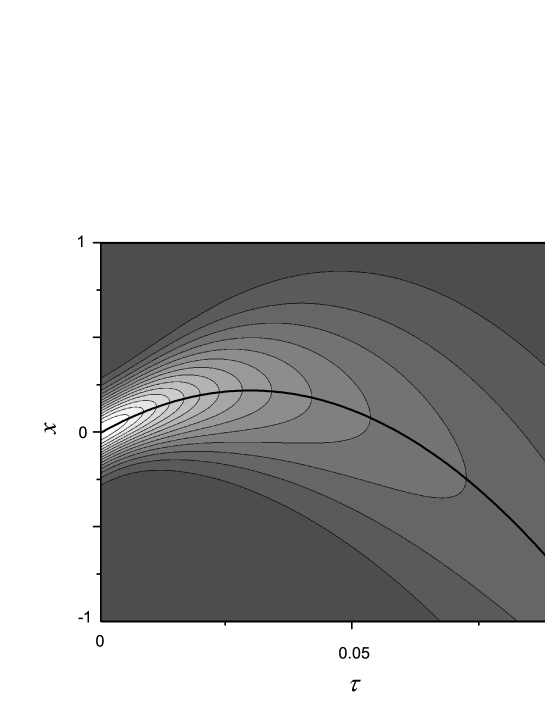
Figure 1: Function $|\psi_{Z}^{c_{1},c_{2}}(\tau;x)|^{2},\;c_{1}=3,\;c_{2}=\sqrt{8},\;x_{0}=0,\;p_{0}=15,\;b=180.$ Plain line represents the parabolic classical trajectory $x(\tau)$ given by (16).

II.1.3 Semi-classical features

Let us calculate some means and dispersions in the CS. To this end, we use relations between the operators $\hat{x}$ and $\hat{p}=-i\partial_{x}$, and the creation and annihilation operators $\hat{A}^{{\dagger}}\left(\tau\right)$ and $\hat{A}\left(\tau\right),$ which follow from (5) and (8),

$$\hat{x}=\frac{1}{\sqrt{2}}\left[(f-g)(\hat{A}^{{\dagger}}-\varphi^{\ast})+(f^{\ast}-g^{\ast})(\hat{A}-\varphi)\right],$$

$$\hat{p}=i\frac{1}{\sqrt{2}}\left[(f+g)(\hat{A}^{+}-\varphi^{\ast})-(f^{\ast}+g^{\ast})(\hat{A}-\varphi)\right].$$ (24)

Then

$$\overline{x}\overset{\mbox{def}}{=}\langle Z,\tau|\hat{x}|Z,\tau\rangle=x(\tau)$$

$$=\frac{1}{\sqrt{2}}\left[Z(f^{\ast}-g^{\ast})+Z^{\ast}(f-g)-2b\tau^{2}\right],$$

$$\overline{p}\overset{\mbox{def}}{=}\langle Z,\tau|\hat{p}|Z,\tau\rangle=p(\tau)=\frac{p_{0}}{2}-\sqrt{2}b\tau.$$ (25)

Let us introduce the deviation operators $\Delta x$ and $\Delta p$,

$$\Delta x=\hat{x}-x(\tau)=$$

$$\frac{1}{\sqrt{2}}\left[(f-g)\left(\hat{A}^{+}-Z^{\ast}\right)+(f^{\ast}-g^{\ast})\left(\hat{A}-Z\right)\right],$$

$$\Delta p=\hat{p}-p(\tau)=$$

$$\frac{i}{\sqrt{2}}\left[(f+g)\left(\hat{A}^{+}-Z^{\ast}\right)-(f^{\ast}+g^{\ast})\left(\hat{A}-Z\right)\right],$$ (26)

and the variances

$$\sigma_{1}=\overline{(\Delta x)^{2}},\ \ \sigma_{2}=\overline{(\Delta p)^{2}},\ \ \sigma_{3}=\frac{1}{2}\overline{(\Delta x\Delta p+\Delta p\Delta x)}.$$ (27)

The latter quantities can be easily calculated:

$$\sigma_{1}=\frac{1}{2}|f-g|^{2},\ \ \sigma_{2}=\frac{1}{2}|f+g|^{2},\ \ \sigma_{3}=\frac{i}{2}(gf^{\ast}-g^{\ast}f).$$ (28)

One can see that the variances do not depend on $Z,$ but depend on the complex numbers $c_{1}$ and $c_{2}$ according to (11). Choosing the numbers $c_{1}$ and $c_{2}$ one can provide any given (at $\tau=0$) value for $\sigma_{1}$ or $\sigma_{2}$. It follows from (28):

$$J=\sigma_{1}\sigma_{2}-\sigma_{3}^{2}=1/4.$$ (29)

The quantity $J$ does not depend on time, it is minimal in the CS.

One ought to mention that for $\alpha=0$ which correspond to the free particle case, the CS (15) coincide with the ones constructed in the work GueLoA11 .

II.2 CS for general potentials

Let the one-dimensional Schrödinger equation have a more general than (1) form

$$i\hbar\frac{\partial\Psi}{\partial t}=\hat{H}\Psi,\ \ \hat{H}=-\frac{\hbar^{2}\partial_{x^{1}}^{2}}{2m}+V\left(x^{1}\right),$$ (30)

where $V\left(x^{1}\right)$ is a potential which corresponds either to a discrete or to a continuous spectrum. Using dimensionless variables $x$ and$\,\tau$ given by (2), we obtain

$$i\frac{\partial\Psi}{\partial\tau}=\hat{H}\Psi,\ \ \hat{H}=-\partial_{x}^{2}+U\left(x\right),\ \ \ U\left(x\right)=\frac{2ml^{2}}{\hbar^{2}}V\left(lx\right).$$ (31)

Let us suppose that we are able to construct an operator $\hat{A}\left(\tau\right)$-integral of motion that obeys the conditions

$$[\hat{S},\hat{A}\left(\tau\right)]=0,\ \ \hat{S}=i\frac{\partial}{\partial\tau}-\hat{H},\ \ \ [\hat{A}\left(\tau\right),\hat{A}^{+}\left(\tau\right)]=1.$$ (32)

Then, we define the vacuum state $|0,\tau\rangle$ for the operator $\hat{A}\left(\tau\right)$ by equation (19), the unitary displacement operator $D\left(Z,\tau\right)$ given by eq. (20), and finally coherent states $D\left(Z,\tau\right)$ by equation (21).

We stress that such a construction is based on the possibility to find a complete discrete set of solutions of the Schrödinger equation with a given potential. Such a possibility naively follows from the existence of a unitary evolution operator in the case under consideration and from the existence of a discrete complete basis in the corresponding Hilbert space (then vectors from such a basis can be chosen as initial states and developed then into a complete set of solutions by the evolution operator). However, we know that the definition domain of the Hamiltonian as a rule does not coincide with the Hilbert space, this is a source of numerous paradoxes (see GVT ) and, in particular, can create difficulties with the realization of the described above program.

For any quadratic potential $U\left(x\right)$ operators $\hat{A}\left(\tau\right)$ and $\hat{A}^{+}\left(\tau\right)$ are expressed by a linear canonical transformation with the creation and annihilation operators $a^{{\dagger}}$ and $a$ given by (5). Coefficient functions in such a canonical transformation obey ordinary differential equations of second order, BagGi90 . For more general potentials one has to elaborate specific methods for solving the operator equations (32). In any case, in the approach under consideration, we are not restricted by the demand that the system has to have a discrete spectrum.

III CS for conservative systems with continuous spectra. An alternative construction

III.1 Pseudo-action & angle variables

We consider again the motion of a particle of mass $m$ on the line, with phase space conjugate variables $(q,p)$, and submitted to a potential $V(q)$. Suppose it conservative. For a given unbounded motion its Hamiltonian function is fixed to a certain value $E$ of the energy:

$$H(q,p)=\frac{p^{2}}{2m}+V(q)=E\,.$$ (33)

Solving this for the momentum variable $p$, assuming a positive velocity, leads to

$$p=p(q,E)=\sqrt{2m}\sqrt{E-V(q)}\,,$$ (34)

supposing no restriction on $q$, e.g. $E-V(q)>0$ for all $q$. From $p=mdq/dt$ we derive the expression of the time as a function of $(q,p)$, through $V$ and from $E=E(q,p)$:

$$dt=\sqrt{\frac{m}{2}}\frac{dq}{\sqrt{E-V(q)}}\quad\Rightarrow$$

$$t-t_{0}=\sqrt{\frac{m}{2}}\int_{q_{0}}^{q}\frac{dq^{\prime}}{\sqrt{E-V(q^{\prime})}}\,.$$ (35)

We then introduce a “pseudo-action” variable, depending on $(q,p)$ through the energy only, $\mathfrak{J}=\mathfrak{J}(E)$, with derivative submitted to the condition

$$\mathfrak{J}^{\prime}(E)=\frac{d\mathfrak{J}}{dE}>0\,.$$ (36)

Thus the map $E\mapsto\mathfrak{J}(E)$ is one-to-one and $E$ can be considered as well as a function of $\mathfrak{J}$: $E=E(\mathfrak{J})$. We now consider the map $(q,p)\mapsto(\mathfrak{J},t)$ with Jacobian matrix

$$\begin{pmatrix}\frac{m}{p}-\frac{V^{\prime}(q)}{2}\sqrt{\frac{m}{2}}\int_{q_{0}}^{q}\frac{dq^{\prime}}{(E-V(q^{\prime 3/2}}&-\frac{p}{2}\sqrt{\frac{1}{2m}}\int_{q_{0}}^{q}\frac{dq^{\prime}}{(E-V(q^{\prime 3/2}}\\ \mathfrak{J}^{\prime}(E)\,V^{\prime}(q)&\mathfrak{J}^{\prime}(E)\,\frac{p}{m}\end{pmatrix}\,,$$ (37)

with determinant equal to $\mathfrak{J}^{\prime}(E)\equiv(F(\mathfrak{J}))^{-1}$. Therefore, the map

$$(q,p)\mapsto(\mathfrak{J},\gamma)\,,\quad\gamma\overset{\mbox{def}}{=}F(\mathfrak{J}(E(q,p))\,t(q,p)\,,$$ (38)

has Jacobian equal to 1, i.e. is canonical. New variables will be called “pseudo-action–angle” variables by analogy with the usual action-angle variable used for bounded one-dimensional motions. Note the role played by $\gamma$ as a kind of intrinsic time for the system, like the angle variable does for bounded motions.

Suppose that measurements on the considered one-dimensional system with classical energy $E=p^{2}/2m+V(q)$ yield the continuous spectral values for the energy observable (up to a constant shift), denoted by $\mathscr{E}$:

$$0\leq\mathscr{E}<\mathscr{E}_{M}\,,\quad\mathscr{E}_{M}\ \mbox{finite or $\infty$}$$ (39)

The difference between the two physical quantities, classical $E$ and quantum $\mathscr{E}$, lies in the probabilistic nature of the measurement of the latter, involving Hilbertian quantum states. Let $\varepsilon$ be a constant characteristic energy of the considered system (e.g. $h/\tau$, where $\tau$ is a characteristic time). We put $\tilde{\mathscr{E}}=\mathscr{E}/\varepsilon$. We define a corresponding sequence of probability distributions $\mathfrak{J}\mapsto p_{\mathscr{E}}(\mathfrak{J})$, $\int_{\mathcal{R}_{\mathfrak{J}}}d\tilde{\mathfrak{J}}\,p_{\mathscr{E}}(\mathfrak{J})=1$, supposing a (prior) uniform distribution on the range $\mathcal{R}_{\mathfrak{J}}$ of the pseudo-action variable $\mathfrak{J}$. Furthermore, we impose $p_{\mathscr{E}}(\mathfrak{J})$ to obey the two conditions:

$$0<\,\mathcal{N}(\mathfrak{J})\overset{\mbox{def}}{=}\int_{0}^{\tilde{\mathscr{E}}_{M}}d\tilde{\mathscr{E}}\,p_{\mathscr{E}}(\mathfrak{J})<\infty\,,$$

$$\mathscr{E}=\int_{\mathcal{R}_{\mathfrak{J}}}d\tilde{\mathfrak{J}}\,E(\mathfrak{J})\,p_{\mathscr{E}}(\mathfrak{J})\,,$$ (40)

where $\tilde{\mathfrak{J}}=\mathfrak{J}/h$, $h$ being the Plank constant. The finiteness condition allows to consider the map $\mathscr{E}\mapsto p_{\mathscr{E}}(\mathfrak{J})/\mathcal{N}(\mathfrak{J})$ as a probabilistic model referring to the continuous energy data, which might viewed in the present context as a prior distribution.

III.2 Pseudo-action-angle coherent states

Let $\mathcal{H}$ be a complex Hilbert space with distributional orthonormal basis $\{|\psi_{\mathscr{E}}\rangle\,,\,0\leq\mathscr{E}<\mathscr{E}_{M}\}$,

$$\langle\psi_{\mathscr{E}}|\psi_{{\mathscr{E}}^{\prime}}\rangle=\delta(\mathscr{E}-\mathscr{E}^{\prime})\,,\ \ \int_{0}^{\tilde{\mathscr{E}}_{M}}d\tilde{\mathscr{E}}\,|\psi_{\mathscr{E}}\rangle\langle\psi_{\mathscr{E}}|=1_{\mathcal{H}}\,.$$ (41)

The pseudo-action-angle phase space for the unbounded motion with measured energies $0\leq\mathscr{E}<\mathscr{E}_{M}$ is the set $X=\{(\mathfrak{J},\gamma)\,,\,\mathfrak{J}\in\mathcal{R}_{\mathfrak{J}}\,,\,\gamma\in\mathbb{R}\}$. Let $\left(p_{\mathscr{E}}(\mathfrak{J})\right)$ be the continuous set of probability distributions associated with these energies. One then constructs the family of states in $\mathcal{H}$ for the considered motion as the following continuous map from $X$ into $\mathcal{H}$:

$$X\ni(\mathfrak{J},\gamma)\mapsto|\mathfrak{J},\gamma\rangle=$$

$$\frac{1}{\sqrt{\mathcal{N}(\mathfrak{J})}}\int_{0}^{\tilde{\mathscr{E}}_{M}}d\tilde{\mathscr{E}}\,\sqrt{p_{\mathscr{E}}(\mathfrak{J})}\,e^{-i\alpha_{\mathscr{E}}\,\gamma}\,|\psi_{\mathscr{E}}\rangle\in\mathcal{H}\,,$$ (42)

where the choice of the real function $\mathscr{E}\mapsto\alpha_{\mathscr{E}}$ is left to us in order to comply with some reasonable physical criteria. A natural choice which guaranties time evolution stability is $\alpha_{\mathscr{E}}=\varsigma\tilde{\mathscr{E}}$, where $\varsigma$ is some constant.

The coherent states $|\mathfrak{J},\gamma\rangle$ are unit vector : $\langle\mathfrak{J},\gamma|J,\gamma\rangle=1$ and resolve the unity operator in $\mathcal{H}$ with respect to the measure “in the Bohr sense” $\mu_{B}(d\mathfrak{J}\,d\gamma)$ on the phase space $X$ :

$$\int_{X}\mu_{B}(d\mathfrak{J}\,d\gamma)\,\mathcal{N}(\mathfrak{J})\,|\mathfrak{J},\gamma\rangle\langle\mathfrak{J},\gamma|\overset{\mbox{def}}{=}$$

$$\int_{\mathcal{R}_{\mathfrak{J}}}d\tilde{\mathfrak{J}}\,\mathcal{N}(\mathfrak{J})\,\lim_{T\to\infty}\frac{1}{T}\int_{-\frac{T}{2}}^{\frac{T}{2}}d\gamma|\mathfrak{J},\gamma\rangle\langle\mathfrak{J},\gamma|=1_{\mathcal{H}}\,.$$ (43)

This property allows a coherent state quantization of classical observables $f(\mathfrak{J},\gamma)$ which is energy compatible with our construction of the posterior distribution $\mathfrak{J}\mapsto p_{\mathscr{E}}(\mathfrak{J})$ in the following sense:

$$f(\mathfrak{J},\gamma)\mapsto\int_{X}\mu_{B}(dJ\,d\gamma)\,\mathcal{N}(\mathfrak{J})\,f(\mathfrak{J},\gamma)\,|\mathfrak{J},\gamma\rangle\langle\mathfrak{J},\gamma|\overset{\mbox{def}}{=}A_{f}\,$$ (44)

Indeed, it is trivially verified that the quantum Hamiltonian is what we expect:

$$A_{H}=\int_{X}\mu_{B}(dJ\,d\gamma)\,\mathcal{N}(\mathfrak{J})\,E(\mathfrak{J})\,|\mathfrak{J},\gamma\rangle\langle\mathfrak{J},\gamma|=$$

$$\int_{0}^{\tilde{\mathscr{E}}_{M}}d\tilde{\mathscr{E}}\,\mathscr{E}|\psi_{\mathscr{E}}\rangle\langle\psi_{\mathscr{E}}|\,,$$

that is, the states $|\psi_{\mathscr{E}}\rangle$ are eigendistributions of the quantum Hamiltonian $A_{H}$ with eigenvalues the elements of the spectrum (39).

The quantization of any function $f(\mathfrak{J})$ of the single pseudo-action variable yields the diagonal operator:

$$f(\mathfrak{J})\mapsto A_{f}=\int_{0}^{\tilde{\mathscr{E}}_{M}}d\tilde{\mathscr{E}}\,\langle f\rangle_{\mathscr{E}}|\psi_{\mathscr{E}}\rangle\langle\psi_{\mathscr{E}}|\,.$$ (45)

where

$$\langle f\rangle_{\mathscr{E}}=\int_{\mathcal{R}_{\mathfrak{J}}}d\tilde{\mathfrak{J}}\,f(\mathfrak{J})\,p_{\mathscr{E}}(\mathfrak{J})\,.$$ (46)

Alternatively, the quantization of any function $f(\gamma)$ of the single angle variable only yields the operator:

$$f(\gamma)\mapsto A_{f}=\int_{0}^{\tilde{\mathscr{E}}_{M}}d\tilde{\mathscr{E}}\int_{0}^{\tilde{E}^{\prime}_{M}}d\tilde{\mathscr{E}}^{\prime}\,[A_{f}]_{\mathscr{E}\mathscr{E}^{\prime}}|\psi_{\mathscr{E}}\rangle\langle\psi_{\mathscr{E}^{\prime}}|\,,$$ (47)

where the matrix elements$[A_{f}]_{\mathscr{E}\mathscr{E}^{\prime}}$ are formally given by:

$$[A_{f}]_{\mathscr{E}\mathscr{E}^{\prime}}=$$

$$\int_{\mathcal{R}_{\mathfrak{J}}}d\tilde{\mathfrak{J}}\,\sqrt{p_{\mathscr{E}}(\mathfrak{J})\,p_{\mathscr{E}^{\prime}}(\mathfrak{J})}\,\lim_{T\to\infty}\frac{1}{T}\int_{-\frac{T}{2}}^{\frac{T}{2}}d\gamma\,e^{-i(\alpha_{\mathscr{E}}-\alpha_{\mathscr{E}^{\prime}})\gamma}\,f(\gamma)\,.$$ (48)

In particular the CS quantization procedure provides, for a given choice of the function $\mathscr{E}\mapsto\alpha_{\mathscr{E}}$, a self-adjoint operator corresponding to any real bounded or semi-bounded function $f(\gamma)$. For instance, the quantization of the elementary Fourier exponential $f(\gamma)=e^{i\varpi\gamma}$ gives a bounded operator with matrix elements (in the considered energy range):

$$[A_{e^{i\varpi\gamma}}]_{\mathscr{E}\mathscr{E}^{\prime}}=\pi\left[\int_{\mathcal{R}_{\mathfrak{J}}}d\tilde{\mathfrak{J}}\,\sqrt{p_{\mathscr{E}}(\mathfrak{J})\,p_{\mathscr{E}^{\prime}}(\mathfrak{J})}\right]\,\delta(\alpha_{\mathscr{E}^{\prime}}-\alpha_{\mathscr{E}}+\varpi)\,.$$ (49)

The quantization of the original canonical position and momentum variables $(q,p)$ is carried out through the functions $q=q(\mathfrak{J},\gamma)$, $p=p(\mathfrak{J},\gamma)$ obtained through the inverse of the map (38). It yields symmetric position and momentum operators. Self-adjointness is not guaranteed, depending or not on the choice of the choice of distribution $\mathfrak{J}\mapsto p_{\mathscr{E}}(\mathfrak{J})$ and the function $\mathscr{E}\mapsto\alpha_{\mathscr{E}}$. It is possible that regularization techniques are needed here.

Semi-classical aspects of such coherent states and related quantization are suitably caught through the so-called lower symbols of operators $A_{f}$, i.e. their mean values in coherent states $\check{f}(\mathfrak{J},\gamma)=\langle\mathfrak{J},\gamma|A_{f}|\mathfrak{J},\gamma\rangle$. As a matter of fact, the map $f\mapsto\check{f}$ is the Berezin-like integral transform

$$\check{f}(\mathfrak{J},\gamma)=\int_{X}\mu_{B}(dJ^{\prime}\,d\gamma^{\prime})\,\mathcal{N}(\mathfrak{J}^{\prime})\,f(\mathfrak{J}^{\prime},\gamma^{\prime})\,|\langle\mathfrak{J}^{\prime},\gamma^{\prime}|\mathfrak{J},\gamma\rangle|^{2}\,,$$ (50)

which gives at once some insight on the domain properties of $A_{f}$ and on the semi-classical behavior of the coherent states.

III.3 An exploration with normal law

Let us choose the following function for the classical pseudo-action:

$$\tilde{\mathfrak{J}}(E)=\eta\ln\tilde{E}\,,\ \Leftrightarrow\ \tilde{E}=e^{\tilde{\mathfrak{J}}/\eta}\,,\quad\eta>0\,,\tilde{E}>0\,,$$ (51)

and so $\mathcal{R}_{\mathfrak{J}}=\mathbb{R}$ for the range of $\mathfrak{J}$. For the probability distribution $\mathfrak{J}\mapsto p_{\mathscr{E}}(\mathfrak{J})$ we choose the normal law centered at $\eta\ln\tilde{\mathscr{E}}$:

$$p_{\mathscr{E}}(\mathfrak{J})=\left(\frac{\epsilon}{\pi}\right)^{1/2}\,e^{-\epsilon(\tilde{\mathfrak{J}}-\eta\ln\tilde{\mathscr{E}})^{2}}\,.$$ (52)

Then the three fundamental requirements are (almost) fulfilled:

• it is probabilistic: $\int_{\mathbb{R}}d\tilde{\mathfrak{J}}\,p_{\mathscr{E}}(\mathfrak{J})=1$,

• the average value of the classical energy is $\approx$ the observed value at large $\epsilon$ or $\eta$:

  $$\int_{\mathbb{R}}d\tilde{\mathfrak{J}}\,E(\mathfrak{J})\,p_{\mathscr{E}}(\mathfrak{J})=e^{\frac{1}{4\epsilon\eta^{2}}}\,\mathscr{E}\,,$$ (53)

• positiveness and finiteness conditions are fulfilled:

  $$0<\,\mathcal{N}(\mathfrak{J})=\int_{0}^{\tilde{\mathscr{E}}_{M}}d\tilde{\mathscr{E}}\,p_{\mathscr{E}}(\mathfrak{J})=\frac{1}{\eta}\,e^{\left(\frac{\tilde{\mathfrak{J}}}{\eta}+\frac{1}{4\epsilon\eta^{2}}\right)}<\infty\,.$$ (54)

Note the average value of $\mathfrak{J}$ : $\int_{\mathbb{R}}d\tilde{\mathfrak{J}}\,\mathfrak{J}\,p_{\mathscr{E}}(\mathfrak{J})=h\eta\ln\tilde{\mathscr{E}}$. Coherent states with $\alpha_{\mathscr{E}}=\varsigma\tilde{\mathscr{E}}$ read as:

$$X=\mathbb{R}\times\mathbb{R}\mapsto$$

$$|\mathfrak{J},\gamma\rangle=\frac{1}{\sqrt{\mathcal{N}(\mathfrak{J})}}\int_{0}^{\infty}d\tilde{\mathscr{E}}\,\sqrt{p_{\mathscr{E}}(\mathfrak{J})}\,e^{-i\varsigma\tilde{\mathscr{E}}\,\gamma}\,|\psi_{\mathscr{E}}\rangle\in\mathcal{H}\,,$$ (55)

They are, by construction, unit vectors, are temporal evolution stable for large $\epsilon$ or $\eta$, and solve the identity:

$$\langle\mathfrak{J},\gamma|\mathfrak{J},\gamma\rangle=1\,,\quad\int_{X}\mu_{B}(d\mathfrak{J}\,d\gamma)\,\mathcal{N}(\mathfrak{J})\,|\mathfrak{J},\gamma\rangle\langle\mathfrak{J},\gamma|=1_{\mathcal{H}}\,,$$

$$\quad e^{-i\tilde{A}_{H}t}|\mathfrak{J},\gamma\rangle=|\mathfrak{J},\gamma+t/\varsigma\rangle\,,$$ (56)

with $\tilde{A}_{H}=A_{H}/h$. They overlap as

$$\langle\mathfrak{J}^{\prime},\gamma^{\prime}|\mathfrak{J},\gamma\rangle=\frac{1}{\sqrt{\mathcal{N}(\mathfrak{J})\mathcal{N}(\mathfrak{J}^{\prime})}}\,e^{-\frac{\epsilon}{4}(\tilde{\mathfrak{J}}-\tilde{\mathfrak{J}}^{\prime})^{2}}\,\left(\frac{\epsilon}{\pi}\right)^{1/2}\,$$

$$\times\int_{0}^{+\infty}d\tilde{\mathscr{E}}\,e^{-i\varsigma\tilde{\mathscr{E}}(\gamma-\gamma^{\prime})}\,e^{-\epsilon\left(\frac{\tilde{\mathfrak{J}}+\tilde{\mathfrak{J}}^{\prime}}{2}-\eta\ln\tilde{\mathscr{E}}\right)^{2}}\,.$$ (57)

This indicates a bell-shaped localization in pseudo-action variable at large $\tilde{\mathfrak{J}}$ or at large $\epsilon$:

$$|\langle\mathfrak{J}^{\prime},\gamma^{\prime}|\mathfrak{J},\gamma\rangle|\leq\frac{1}{\sqrt{\mathcal{N}(\mathfrak{J})\mathcal{N}(\mathfrak{J}^{\prime})}}\,e^{-\frac{\epsilon}{4}(\tilde{\mathfrak{J}}-\tilde{\mathfrak{J}}^{\prime})^{2}}\,\left(\frac{\epsilon}{\pi}\right)^{1/2}\,$$

$$\times\int_{0}^{+\infty}d\tilde{\mathscr{E}}\,e^{-\epsilon\left(\frac{\tilde{\mathfrak{J}}+\tilde{\mathfrak{J}}^{\prime}}{2}-\eta\ln\tilde{\mathscr{E}}\right)^{2}}\,.$$ (58)

A similar good localization in angle requires a study of the behavior at large $k$ of the following Fourier transform: $\int_{0}^{+\infty}dxe^{-ikx}\,e^{-\mu(\ln x-\lambda)^{2}}\,,$ with $x=\tilde{\mathscr{E}}$, $k=\varsigma(\gamma-\gamma^{\prime})$, $\mu=\epsilon\eta^{2}$, and $\lambda=\frac{\tilde{\mathfrak{J}}+\tilde{\mathfrak{J}}^{\prime}}{2\eta}$.

An interesting observation concerns the CS quantization of any power of the classical energy:

$$A_{H^{\lambda}} =\int_{X}\mu_{B}(dJ\,d\gamma)\,\mathcal{N}(\mathfrak{J})\,(E(\mathfrak{J}))^{\lambda}\,|\mathfrak{J},\gamma\rangle\langle\mathfrak{J},\gamma|$$

$$=e^{\frac{\lambda^{2}}{4\epsilon\eta^{2}}}\int_{0}^{+\infty}d\tilde{\mathscr{E}}\,(\mathscr{E})^{\lambda}|\psi_{\mathscr{E}}\rangle\langle\psi_{\mathscr{E}}|\,,$$

which means that $A_{H^{\lambda}}=e^{\frac{\lambda(\lambda-1)}{4\epsilon\eta^{2}}}\left(A_{H}\right)^{\lambda}$. The quantization of the Fourier exponential $e^{i\varpi\gamma}$ gives the bounded operator

$$A_{e^{i\varpi\gamma}}=\frac{\pi}{\varsigma}\int_{\sup(0,\varpi/\varsigma)}^{+\infty}e^{-\frac{\epsilon\eta}{4}\left(\ln\left(\frac{\tilde{\mathscr{E}}}{\tilde{\mathscr{E}}-\varpi/\varsigma}\right)\right)^{2}}\,|\psi_{\mathscr{E}}\rangle\langle\psi_{\mathscr{E}-\varpi/\varsigma}|\,.$$ (59)

We might be able to deduce from this formula the quantization of the variable $\gamma$ by the formal trick $A_{\gamma}=\left.-i\partial/\partial\varpi A_{e^{i\varpi\gamma}}\right|_{\varpi=0}$.

III.4 Probability distributions on phase or other spaces

In Figure 2 are shown two-dimensional pictures of the probability density $\mathcal{N}(\mathfrak{J})|\langle\mathfrak{J}^{\prime},\gamma^{\prime}|\mathfrak{J},\gamma\rangle|^{2}$ with

$$\mathcal{N}(\mathfrak{J})=\int_{0}^{\tilde{\mathscr{E}}_{M}}d\tilde{\mathscr{E}}\,p_{\mathscr{E}}(\mathfrak{J})=\frac{1}{\eta}\,e^{\left(\frac{\tilde{\mathfrak{J}}}{\eta}+\frac{1}{4\epsilon\eta^{2}}\right)}$$ (60)

and,

$$\langle\mathfrak{J}^{\prime},\gamma^{\prime}|\mathfrak{J},\gamma\rangle=\frac{1}{\sqrt{\mathcal{N}(\mathfrak{J})\mathcal{N}(\mathfrak{J}^{\prime})}}\,e^{-\frac{\epsilon}{4}(\tilde{\mathfrak{J}}-\tilde{\mathfrak{J}}^{\prime})^{2}}\,\left(\frac{\epsilon}{\pi}\right)^{1/2}\,$$

$$\times\int_{0}^{+\infty}d\tilde{\mathscr{E}}\,e^{-i\varsigma\tilde{\mathscr{E}}(\gamma-\gamma^{\prime})}\,e^{-\epsilon\left(\frac{\tilde{\mathfrak{J}}+\tilde{\mathfrak{J}}^{\prime}}{2}-\eta\ln\tilde{\mathscr{E}}\right)^{2}}\,.$$ (61)

We fix the parameters $(\mathfrak{J},\gamma)$ and sweep $(\mathfrak{J}^{\prime},\gamma^{\prime})$ in the $\mathbb{R}\times\mathbb{R}$ space. Parameters $\epsilon=\eta=\varsigma=\mathfrak{J}=1$ are chosen for an example. That gives a nice picture of the expected good localization of these states in the phase space plane $(\mathfrak{J}^{\prime},\gamma^{\prime})$.

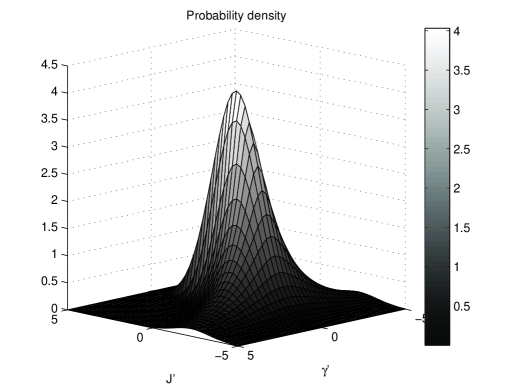
Figure 2: Calculated phase space probability density (Eq. III.4) with $\mathfrak{J}=\gamma=0$, $\varsigma=\epsilon=\eta=1$ and zoom in the range $\mathfrak{J}^{\prime}:-5\div 5\,,\quad\gamma^{\prime}:-5\div 5$.

Let us explore another representation, picking $\mathcal{H}=L^{2}(\mathbb{R})$ as a companion Hilbert space and as continuous basis the eigen-distributions of the operator $-d^{2}/d\mathsf{x}^{2}$ GVT : to each eigenvalue $\tilde{\mathscr{E}}$ correspond the symmetric $\psi_{\mathscr{E}}^{+}(\mathsf{x})=\frac{1}{\sqrt{4\pi\sqrt{\tilde{\mathscr{E}}}}}\cos(\sqrt{\tilde{\mathscr{E}}}\mathsf{x})$ and the antisymmetric $\psi_{\mathscr{E}}^{-}(\mathsf{x})=\frac{-i}{\sqrt{4\pi\sqrt{\tilde{\mathscr{E}}}}}\sin(\sqrt{\tilde{\mathscr{E}}}\mathsf{x})$ (the phase $-i$ is chosen for convenience). A degeneracy of order 2 is present here and should be taken into account by including a factor 2 in the spectral measure $d\tilde{\mathscr{E}}|\psi_{\mathscr{E}}\rangle\langle\psi_{\mathscr{E}}|$ appearing in (41). We should caution against the risk of confusion with the position representation: the symbol $\mathsf{x}$ should not be regarded in general as an element of the spectrum of the position operator $A_{q}$, and instead, we should view the states (III.3) as special wave packets in representation “$\mathsf{x}$”. We find from (III.3) (after the change $u=\sqrt{\tilde{\mathscr{E}}}$),

$$\langle\mathsf{x}|\mathfrak{J},\gamma\rangle=\sqrt{\frac{\epsilon\eta^{2}}{\pi^{3}}}\,e^{-\frac{\epsilon}{2}\left(\tilde{\mathfrak{J}}+\frac{1}{2\epsilon\eta}\right)^{2}}$$

$$\times\int_{0}^{+\infty}du\,u^{2\epsilon\eta\tilde{\mathfrak{J}}+1/2}\,e^{-2\epsilon\eta^{2}(\ln u)^{2}}\,e^{-i(\varsigma\gamma u^{2}+u\mathsf{x})}\,,$$ (62)

The study of this expression amounts to analyze the behavior of the following Fourier transform:

$$F(\mathsf{x})=\frac{1}{\sqrt{2\pi}}\int_{0}^{+\infty}du\,e^{-i\mathsf{x}u}\,u^{\alpha}\,e^{-\delta(\ln u)^{2}}\,e^{-i\beta u^{2}}\,,$$ (63)

with $\alpha=2\epsilon\eta\tilde{\mathfrak{J}}+1/2$, $\beta=\varsigma\gamma$, and $\delta=2\epsilon\eta^{2}$. From the upper bound

$$|F(\mathsf{x})|\leq\sqrt{\frac{2}{\delta}}\,e^{\frac{(\alpha+1)^{2}}{4\delta}}\,,$$ (64)

we see that it can be made arbitrarily small at large $\eta$. The map

$$\mathsf{x}\mapsto|\langle\mathsf{x}|\mathfrak{J},\gamma\rangle|^{2}=\frac{\epsilon\eta^{2}}{\pi^{3}}\,e^{-\epsilon\left(\tilde{\mathfrak{J}}+\frac{1}{2\epsilon\eta}\right)^{2}}$$

$$\times\left|\int_{0}^{+\infty}du\,u^{2\epsilon\eta\tilde{\mathfrak{J}}+1/2}\,e^{-2\epsilon\eta^{2}(\ln u)^{2}}\,e^{-i(\varsigma\gamma u^{2}+\mathsf{x}u)}\right|^{2}$$ (65)

defines a probability distribution on the real line. As shown in Figure 3, it gives an insight into the localization of the coherent states viewed as wave packets on the line $\mathsf{x}\in\mathbb{R}$ and their spreading in function of the rescaled “time” $\gamma$.

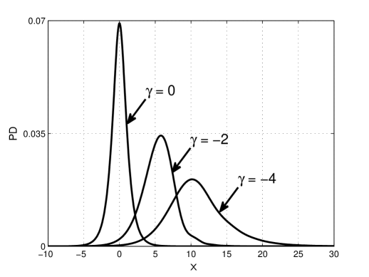
Figure 3: Calculated probability densities (Eq. III.4) on the real line $\mathsf{x}\in\mathbb{R}$ with $\mathfrak{J}=0$, $\varsigma=\epsilon/2=\eta=1$, for the values $\gamma=-4,\,-2,\,0$. One can notice the spreading of the wave packet.

IV Conclusion

We have presented two methods for constructing families of coherent states adapted to the quantum description of unbounded motions on the real line.

The first approach follows the Malkin-Manko treatment of quadratic Hamiltonians and is more of algebraic nature, resting upon canonical commutation rules and invariance principles. We have considered the example of a particle submitted to a constant force (i.e. linear potential) and obtained families of states fulfilling semi-classical exigences. We have also given some insight about generalization to arbitrary potentials.

The second approach is of probabilistic nature. It provides a broad range of possibilities in choosing the three main ingredients of the CS construction: the function $E\mapsto\mathfrak{J}(E)$ on a classical level, and, on a quantum level, the probability distributions $\mathfrak{J}\mapsto p_{\mathscr{E}}(\mathfrak{J})$ and the frequency function $\mathscr{E}\mapsto\alpha_{\mathscr{E}}$. Of course, the selection should be ruled by the requirement of manageable quantum operators combined with acceptable semi-classical properties.

In a next publication we will examine in a more comprehensive way the following points:

• generalization of the first method to arbitrary potentials,

• algebraic and domain properties of position and momentum operators yielded by the second approach,

• detailed comparison of the two approaches with regard to localization properties in phase space and in configuration space.

References

• (1) Special issue on coherent states: mathematical and physical aspects S. T. Ali, J.-P. Antoine, F. Bagarello and J.-P. Gazeau (Ed.), J. Phys. A, to appear (2012).
• (2) R. Glauber, Phys. Rev. Lett. 10 84- (1963); Phys. Rev. 130 2529- (1963); J.R.Klauder, E.C.Sudarshan, Fundamentals of Quantum Optics, (Benjamin, 1968)
• (3) I.A.Malkin, V.I.Man’ko, Dynamical Symmetries and Coherent States of Quantum Systems, (Nauka, Moscow, 1979) pp.320; Soviet Phys. JETP 28 (1969) 527
• (4) R. Gilmore, Geometry of symmetrized states, Ann. Phys. (NY) 74 391-463 (1972).
• (5) A. M. Perelomov, Coherent states for arbitrary Lie groups, Commun. Math. Phys. 26 222-236 (1972).
• (6) A.M.Perelomov, Generalized Coherent States and Their Applications, Springer-Verlag, 1986.
• (7) S.T. Ali, J-P. Antoine, and J-P. Gazeau, Coherent States, Wavelets and Their Generalizations, Springer-Verlag, New York, Berlin, Heidelberg, 2000.
• (8) J.P. Gazeau and J. Klauder, Coherent States for Systems with Discrete and Continuous Spectrum, J. Phys. A: Math. Gen., 32, 123-132 (1999).
• (9) S.T. Ali, B. Heller and J.P. Gazeau, Coherent states and Bayesian duality, J. Phys. A: Math. Theor., 41, 365302 1-22 (2008).
• (10) J.P. Gazeau, Coherent States in Quantum Physics, Wiley-VCH, Berlin, 2009.
• (11) F. A. Berezin, General concept of quantization, Comm. Math. Phys., 40, 153 (1975).
• (12) J.R. Klauder, Quantization Without Quantization, Ann. Phys. (NY) 237, 147-160 (1995).
• (13) J.R. Klauder. Beyond Conventional Quantization. Cambridge University Press, Cambridge, 2000.
• (14) M. Hongoh, Coherent states associated with the continuous spectrum of noncompact groups, J. Math. Phys., 18, 2081-2085 (1977).
• (15) J. Ben Geloun and J. R. Klauder, Ladder operators and coherent states for continuous spectra, J. Phys. A: Math. Theor., 42, 375209 (2009).
• (16) J. Guerrero, F.F. Lûpez-Ruiz, V. Aldaya and F. Cossio, Harmonic states for the free particle, J. Phys. A 44 445307, 1–26 (2011).
• (17) D.M. Gitman, I.V. Tyutin, B.L. Voronov, Self-adjoint Extensions in Quantum Mechanics. General theory and applications to Schroedinger and Dirac equations with singular potentials, Birkhäuser Publisher (2012) in press.
• (18) V.G. Bagrov and D.M. Gitman, Exact Solutions of Relativistic Wave Equations, Math. its Appl., Sov. ser., Vol 39 (Kluwer, Dordrecht 1990)
• (19) J.P. Gazeau and R. Kanamoto, Action-angle coherent states and related quantization, arXiv:1110.6678v1 [quant-ph]