Ground-based, Near-infrared Exospectroscopy. II. Tentative Detection of Emission From the Extremely Hot Jupiter WASP-12b

Abstract

We report the tentative detection of the near-infrared emission of the Hot Jupiter WASP-12b with the low-resolution prism on IRTF/SpeX. We find a $K-H$ contrast color of $0.137\,\%\pm 0.054\,\%$, corresponding to a blackbody of temperature $2400^{+1500}_{-500}~{}\textrm{K}$ and consistent with previous, photometric observations. We also revisit WASP-12b’s energy budget on the basis of secondary eclipse observations: the dayside luminosity is a relatively poorly constrained $(2.0-4.3)\times 10^{30}$ erg s^-1, but this still allows us to predict a day/night effective temperature contrast of $200-1$,000 K (assuming $A_{B}=0$). Thus we conclude that WASP-12b probably does not have both a low albedo and low recirculation efficiency. Our results show the promise and pitfalls of using single-slit spectrographs for characterization of extrasolar planet atmospheres, and we suggest future observing techniques and instruments which could lead to further progress. Limiting systematic effects include the use of a too-narrow slit on one night – which observers could avoid in the future – and chromatic slit losses (resulting from the variable size of the seeing disk) and variations in telluric transparency – which observers cannot control. Single-slit observations of the type we present remain the best option for obtaining $\lambda>1.7\,\micron$ spectra of transiting exoplanets in the brightest systems. Further and more precise spectroscopy is needed to better understand the atmospheric chemistry, structure, and energetics of this, and other, intensely irradiated planet.

1. Introduction

1.1. Ground-based Characterization of Exoplanet Atmospheres

Transiting extrasolar planets allow the exciting possibility of studying the intrinsic physical properties of these planets. The last several years have seen rapid strides in this direction, with measurements of precise masses and radii, detection of numerous secondary eclipses and phase curves, and the start of ground-based optical spectroscopy (Redfield et al., 2008; Snellen et al., 2008; Bean et al., 2010).

Though ground-based, near-infrared (NIR) photometry of exoplanets is becoming commonplace, until recently there were no successful detections via ground-based NIR spectroscopy (Brown et al., 2002; Richardson et al., 2003; Deming et al., 2005; Barnes et al., 2007; Knutson et al., 2007). Several groups have employed high-resolution spectrographs with some form of template cross-correlation (Deming et al., 2005; Snellen et al., 2010; Crossfield et al., 2011) with varying degrees of success. Though cross-correlation provides a method to test for the detection of a particular model, it has the significant drawback that it does not provide a model-independent measurement. Furthermore, such observations require high-resolution cryogenic spectrographs on large-aperture telescopes.

The only published, model-independent, ground-based, NIR spectrum of an exoplanetary atmosphere (Swain et al., 2010) was obtained with a different approach: medium-resolution spectroscopy of HD 189733b with the 3 m NASA Infrared Telescope Facility (IRTF) covering the K and L bands. However, these results are in dispute: the K band matches HST/NICMOS observations which have in turn been called into question (see Swain et al., 2008; Sing et al., 2009; Gibson et al., 2011; Deroo et al., 2010), while the L band exhibits an extremely high flux peak attributed variously to non-LTE $\textrm{CH}_{4}$ emission (Swain et al., 2010) and to contamination by telluric water vapor (Mandell et al., 2011). In contrast, the tentative spectroscopic detection of WASP-12b we present in this paper reproduces previous, high S/N ground-based photometry (Croll et al., 2011) and we demonstrate that our final result is not likely to be corrupted by telluric variations outside of well-defined spectral regions.

1.2. The WASP-12 System

The transiting Hot Jupiter WASP-12b has an orbital period of 1.1 days around its 6300 K host star, and the planet’s mass and radius give it a bulk density only 25% of Jupiter (Hebb et al., 2009; Chan et al., 2011). The planet is one of the largest known and is significantly overinflated compared to standard interior models (Fortney et al., 2007). The planet is significantly distorted and may be undergoing Roche lobe overflow (Li et al., 2010), but tidal effects are not expected to be a significant energy source. Though the initial report suggested WASP-12b had a nonzero eccentricity, subsequent orbital characterization via timing of secondary eclipses (Campo et al., 2011) and further radial velocity measurements (Husnoo et al., 2011) suggest an eccentricity consistent with zero.

WASP-12b is intensely irradiated by its host star, making the planet one of the hottest known and giving it a favorable ($\gtrsim 10^{-3}$) NIR planet/star flux contrast ratio; it has quickly become one of the best-studied exoplanets. The planet’s large size, low density, and high temperature have motivated an ensemble of optical, (López-Morales et al., 2010), NIR (Croll et al., 2011), and mid-infrared (Campo et al., 2011) eclipse photometry which suggests this planet has an unusual carbon to oxygen (C/O) ratio greater than one (Madhusudhan et al., 2011).

However, a wide range of fiducial atmospheric models fit WASP-12b’s photometric emission spectrum equally well despite differing significantly in atmospheric abundances and in their temperature-pressure profiles (Madhusudhan et al., 2011). Many hot Jupiters appear to have high-altitude temperature inversions (Knutson et al., 2010; Madhusudhan & Seager, 2010), but even WASP-12b’s precise, well-sampled photometric spectrum does not constrain the presence or absence of such an inversion. Thus significant degeneracies remain; this is a common state of affairs in the field at present even for such relatively well-characterized systems (Madhusudhan & Seager, 2010). This is because (a) broadband photometry averages over features caused by separate opacity sources and (b) atmospheric models have many more free parameters than there are observational constraints. Spectroscopy, properly calibrated, can break some of these degeneracies, test the interpretation of photometric observations at higher resolution, and ultimately has the potential to more precisely refine estimates of atmospheric abundances, constrain planetary temperature structures, and provide deeper insight into high-temperature exoplanetary atmospheres.

1.3. Outline

This paper presents our observations and analysis of two eclipses of WASP-12b in an attempt to detect and characterize the planet’s NIR emission spectrum. This is part of our ongoing effort to develop the methods necessary for robust, repeatable ground-based exoplanet spectroscopy, and we use many of the same techniques introduced in our first paper (Crossfield et al., 2011, hereafter Paper I).

We describe our spectroscopic observations and initial data reduction in Sec. 2. The data exhibit substantial correlated variability, and we describe our measurements of various instrumental variations in Sec. 3. We fit a simple model that includes astrophysical, instrumental, and telluric effects to the data in Sec. 4. Chromatic slit losses (resulting from wavelength-dependent atmospheric dispersion and seeing) and telluric transmittance and radiance effects can confound ground-based NIR observations, so in Sec. 5 we investigate these systematic error sources in detail. We present our main result – a tentative detection of WASP-12b’s emission – in Sec. 6 and compare it to previous observations. Finally, we discuss the implications of our work for future ground-based, NIR spectroscopy in Sec. 7 and conclude in Sec. 8.

2. Observations and Initial Reduction

2.1. Summary of Observations

We observed the WASP-12 system with the SpeX near-infrared spectrograph (Rayner et al., 2003), mounted at the IRTF Cassegrain focus. Our observations during eclipses on 28 and 30 December 2009 (UT) comprise a total of 10.2 hours on target and 8.3 hours of integration time. We list the details of our observations and our instrumental setup in Table 1. One of our eclipses overlaps one of those observed by Croll et al. (2011) with broadband photometry from the Canada-France-Hawaii Telescope (CFHT), also on Mauna Kea, on UT 27-29 December 2009. Our first night, 28 Dec, is the same night as their H band observation.

Table 1 Observations

UT date	2009 Dec 28	2010 Dec 30
Instrument Rotator Angle	225∘	225∘
Slit Position Angle	90∘	90∘
Slit	1.6” x 15”	3.0” x 15”
Grating	LowRes15	LowRes15
Guiding filter	J	K
OS filter	open	open
Dichroic	open	open
Integration Time (sec)	15	20
Non-destructive reads	4	4
Co-adds	2	2
Exposures	502	356
Airmass range	1.01 - 1.91	1.01 - 2.70
Wavelength coverage ($\mu$m)	$<1$ - 2.5 µm	$<1$ - 2.5 µm
WASP-12b phase coverage	0.42 - 0.61	0.41 - 0.61

On both nights we observed the WASP-12 system continuously for as long as conditions permitted using SpeX’s low-resolution prism mode, which gives uninterrupted wavelength coverage from $<1-2.5$ µm. We chose prism mode because it offers roughly twice the throughput of to SpeX’s echelle modes (Rayner et al., 2003, their Fig. 7), though it has a necessarily reduced capability to spectrally resolve, separate, and mitigate telluric features. We nodded the telescope along the slit to remove the sky background; as we discuss below, this induced substantial flux variations in our spectrophotometry at shorter wavelengths and we urge future exoplanet observers to eschew nodding at these wavelengths (the exception to this rule would be for instruments that suffer from time-varying scattered light, such as SpeX’s short-wavelength cross-dispersed mode). We deactivated the instrument’s field rotator to minimize instrumental flexure, but this meant the slit did not track the parallactic angle and atmospheric dispersion (coupled with variable seeing and telescope guiding errors) causes large-scale, time-dependent, chromatic gradients throughout the night. As we describe in Sec. 5.2 and 5.3, this effect is reduced (but not eliminated) by using a wider slit, and we strongly advise that future observations covering a large wavelength range (a) use as large a slit as possible and (b) keep the slit aligned to the parallactic angle.

On our first night, 28 Dec, we observed with the 1.6” slit to strike a balance between sky background and frame-to-frame variations in the amount of light entering the slit. After this run an initial analysis suggested we could further decrease spectrophotometric variability without incurring significant penalties from sky background, and so we used the 3.0” slit on the second night (30 Dec).

WASP-12 is sufficiently bright (K=10.2) that we were able to guide on the faint ghost reflected from the transmissive, CaF slit mask into the NIR slit-viewing guide camera. Guiding kept the K band relatively stationary but because SpeX covers such a wide wavelength range the spectra suffer from differential atmospheric refraction; this results in substantially larger motions over the course of the night at shorter wavelengths. We did not record guide camera frames, but we recommend that future observers save all such data to track guiding errors, measure the morphology of the two-dimensional point spread function, and measure the amount of light falling outside the slit. Typical frames had maximum count rates of $\lesssim$2,000 ADU pix^-1 coadd^-1, safely within the $1024^{2}$ Aladdin 3 InSb detector’s linear response range.

2.2. Initial Data Reduction

We reduce the raw echelleograms using the SpeXTool reduction package (Cushing et al., 2004), supplemented by our own set of Python analysis tools. SpeXTool dark-subtracts, flat-fields, and corrects the recorded data for detector nonlinearities, and we find it to be an altogether excellent reduction package that future instrument teams would do well to emulate. We used SpeXTool in optimal “A$-$B” point source extraction mode with extraction and aperture radii of 2.5”, inner and outer background aperture radii of 2.8” and 3.5”, respectively, and a linear polynomial to fit and remove the residual background in each column.

The extracted spectra have H and K band fluxes of $\sim$5500 and $\sim$2000 e^- pix^-1 s^-1, respectively. After removing observations rendered unusable for telescope or instrumental reasons (e.g., loss of guiding or server crashes), we are left with 502 and 356 usable frames from our two nights. The extracted spectra are shown in Fig. 1 and substantial variations are apparent; we discuss these in Sec. 3.

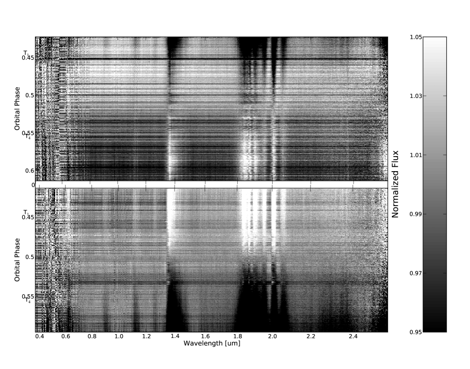
Figure 1.— Spectrophotometric data for the nights of 28 Dec 2009 (top) and 30 Dec 2009 (bottom); each column has been normalized by its median value. The variations (due to a combination of airmass effects and instrumental slit loss) are largely common mode; variations are less on 30 Dec, probably because of the wider slit used then. The first ($T_{1}$) and fourth ($T_{4}$) points of contact of the eclipse are indicated, as calculated from the ephemeris of Hebb et al. (2009).

SpeX typically uses a set of arc lamps for wavelength calibration, but SpeXTool fails to process arcs taken with the 3” slit in prism mode. Instead, we calculate wavelength solutions by matching observed telluric absorption features with an empirical high-resolution telluric absorption spectrum (Hinkle et al., 2003) convolved to the approximate spectral resolution of our observations. We estimate a precision of 1.7 nm for the individual line positions and use this uncertainty to calculate the $\chi^{2}$ and Bayesian Information Criterion (BIC) for fits using successively higher degrees of polynomials: for both nights a fourth-order polynomial gives the lowest BIC, indicating this to be the preferred model. The RMS of the residuals to these fits are 1.3 and 1.6 nm for 28 Dec and 30 Dec, respectively, while maximum residuals for each night are 3.1 nm (at 2.35 µm) and 2.9 nm (at 1.3, 1.85, and 2.32 µm), respectively.

Our wavelength solutions for 28 and 30 Dec are respectively

$$\lambda_{28}(p)/\micron = 6.77626638\times 10^{-12}p^{4}-9.82847002\times 10^{-9}p^{3}+$$

$$2.52383166\times 10^{-6}p^{2}+4.26945216\times 10^{-3}p+$$

$$0.414989079$$

and

$$\lambda_{30}(p)/\micron = 4.85652782\times 10^{-12}p^{4}-6.49601098\times 10^{-9}p^{3}+$$

$$4.97530220\times 10^{-7}p^{2}+4.78270230\times 10^{-3}p+$$

$$0.371045967$$

where $p$ is the pixel number, an integer from 0 to 563, inclusive. We apply these wavelength solutions to all our spectra after shifting them to a common reference frame using the shift-and-fit technique described by Deming et al. (2005) and implemented in Paper I.

3. Characterization of Systematic Effects

3.1. Instrumental Sources

The initially extracted spectra shown in Fig. 1 exhibit temporal variations due to a combination of telluric, instrumental, and astrophysical sources, with the last of these the weakest of the three effects. We wish to quantify and remove the instrumental and telluric effects to the extent that we can convincingly detect any astrophysical signature – i.e., a secondary eclipse. The strongest variations in Fig. 1 are largely common-mode (i.e., they appear in all wavelength channels) and are due to variations in light coupled into the spectrograph due to changes in seeing, pointing, and/or telluric transparency. Longer-term telluric variations are distinguishable by the manner in which they increase in severity in regions of known telluric absorption.

We approximate the amount of light coupled into the spectrograph slit by measuring the flux in regions clear of strong telluric absorption, as determined using our high-resolution telluric absorption spectrum (Hinkle et al., 2003) convolved to our approximate resolution. The flux in these channels should only depend on the frame-to-frame changes in starlight entering the spectrograph slit, which in turn depends on the (temperature- and pressure-dependent) atmospheric dispersion, the (wavelength-dependent) size and shape of the instrumental response, telescope guiding errors, and achromatic changes in telluric transparency. In the interests of simplicity we initially treat this as a wavelength-independent quantity; we return to address the validity and limitations of this assumption in Sec. 5.2.

At each time step we sum the flux in these telluric-free parts of each spectrum, creating a time series representative of the achromatic slit losses suffered by the instrument. Although we refer to this quantity as the slit loss, it is actually a combination of instrumental slit losses (spillover) and changing atmospheric transmission. The achromatic slit loss time series is plotted for each night in Figs. LABEL:fig:dec28_state_vectors and LABEL:fig:dec30_state_vectors, along with other candidate systematic sources described below. We ultimately compute this quantity by summing the flux between $1.63-1.73\,\micron$ and $2.10-2.21\,\micron$, spectral regions we show in Sec. 5.1 to be mostly free of telluric contamination.

Figure 2.— width=3.5in

The observable quantities (described in Sec. 2.2) measured during the course of our observations on 28 Dec 2009. As described in the text, we ultimately detrend our observations with a combination the airmass reported by the telescope control system and the nod position vector. As noted in the text we measure the seeing FWHM and $y$ position as a function of wavelength, but here we plot only the approximate K-band values of these quantities. The dashed lines indicate the four points of contact of the eclipse as calculated from the ephemeris of Hebb et al. (2009).

Figure 3.— width=3.5in

Same as Fig. LABEL:fig:dec28_state_vectors, but for the night of 30 Dec 2009.

SpeX is a large instrument and is mounted at the IRTF’s Cassegrain focus, where its spectra can exhibit several pixels of flexure due to changing gravity vector; similarly, atmospheric dispersion (Filippenko, 1982) introduces many pixels of motion at shorter wavelengths (because we keep the star in the slit by guiding at K band). Apparent spectrophotometric variations can be induced by such instrumental changes (e.g., Knutson et al., 2007, Paper I). We measure the motion of the spectral profiles in the raw frames perpendicular to ($x$) and parallel to ($y$) the long axis of the spectrograph slit as follows. We compute the $x$ motion of the star on the slit while aligning the spectra to a common reference frame as described in Sec. 2.2 above. For $y$ we fit Gaussian profiles to the raw spectral traces, then fit a low-order polynomial to the measured positions in each frame. The $x$ and $y$ motions are typically 2-4 pixels in K band and are plotted for both nights in Figs. LABEL:fig:dec28_state_vectors and LABEL:fig:dec30_state_vectors. An independent method to measure the $x$ and $y$ motions would be to use images recorded by SpeX’s slit-viewing camera: since the slit is slightly reflective one would then be able to measure directly the star’s position on the slit at the guiding wavelength. We recommend observers investigate this approach in the future.

We measure the full-width at half maximum (FWHM) of the spectral profiles during the spectral fitting and tracing described above. Again, we fit a low-order polynomial to the measured values to smoothly interpolate the compute values. The value we measure (which does not scale as $\lambda^{-1/5}$ as would be expected from atmospheric Kolmogorov turbulence; Quirrenbach, 2000) presumably depends on a combination of atmospheric conditions, instrumental focus, and pointing jitter during an exposure, but we hereafter refer to it merely as seeing.

Previous studies (Deming et al., 2005, Paper I) report that an empirical measure of atmospheric absorption is preferable to the calculated airmass value when accounting for telluric extinction. We measured the flux in a number of telluric absorption lines for the species CO₂, $\textrm{CH}_{4}$, and H₂O in a manner similar to that in Paper I. However, in our empirical airmass terms we still see substantial contamination from both slit losses and A/B nodding, and so in our final analysis we use the airmass values reported by the telescope control system and plotted in Figs. LABEL:fig:dec28_state_vectors and LABEL:fig:dec30_state_vectors.

3.2. Slit Loss Effects

Absolute spectrophotometry is difficult with narrow slits because guiding errors, seeing variations, and (when the slit is not aligned to the parallactic angle) atmospheric dispersion, all result in a time-varying amount of starlight coupled into the spectrograph slit (e.g., Knutson et al., 2007, Paper I). After extracting the spectra, our next step is to remove the large-scale flux variations present in the data.

As described in Sec. 5.2 we try to empirically calibrate the amount of light entering the spectrograph slit. Despite considerable effort, we are only able to qualitatively match the variability in our observations. This could be because the PSF morphology (and especially the wavelength-dependent flux ratio between the core and wings) cannot be accurately modeled using a simple Gaussian function (perhaps due to alignment errors within SpeX and/or guiding errors), because our implementation of the simplified formulation of Green (1985) does not reflect reality with sufficient fidelity, or because variations due to telluric sources overwhelm those due to instrumental effects. An independent test could be performed in future efforts by recording images from the slit-viewing camera and directly measuring the light not entering the slit, the shape of the PSF, and its position.

Instead, following Paper I we divide the flux in every wavelength channel by a wavelength-independent slit loss time series. This step removes the absolute eclipse depth (the mean depth over the slit loss wavelength range) from all spectral channels, but the overall shape of the emission spectrum should remain the same. However, the quality of this correction will degrade rapidly at shorter wavelengths because air’s refractive index increases rapidly at shorter wavelength. Especially with a narrow slit (as during our 28 Dec observations) or at high airmass (as on 30 Dec), this can cause a greater proportion of the short-wavelength flux to fall outside the slit. Nonetheless, we are unwilling to venture beyond removal of this simple achromatic trend, given our inability to accurately model the chromatic slit loss component.

Dividing the data by this time series substantially reduces the variability in regions clear of telluric absorption, as shown in Figs. 4, LABEL:fig:dec28_phot, and LABEL:fig:dec30_phot. Note however that some correlated variability remains even after this correction step, as seen for example near orbital phase 0.45 on 28 Dec (Figs. 4 and LABEL:fig:dec28_phot). These residual variations are wavelength-dependent, and support our conclusion that chromatic slit losses are affecting our data. Wider slits should reduce this effect, and indeed such chromatic residuals are reduced by a factor of $\sim 2$ on 30 Dec (see Fig. 4), when we used the wider slit.

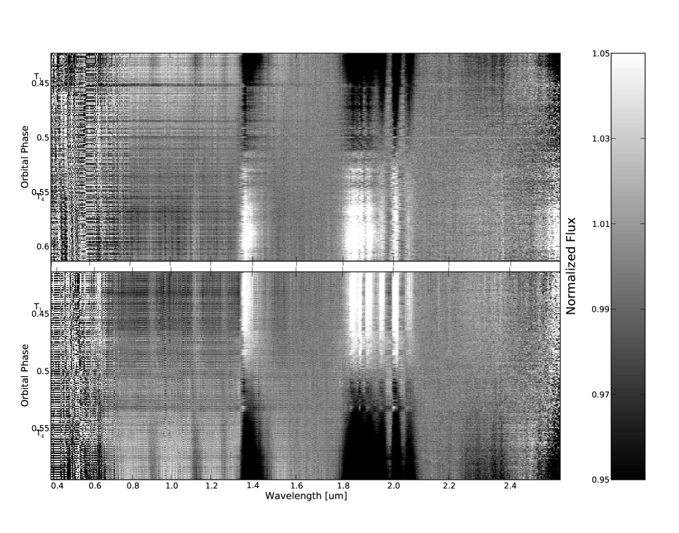
Figure 4.— Spectrophotometric data for the nights of 28 Dec (top) and 30 Dec (bottom) after dividing all wavelength channels by the achromatic slit loss time series and normalized by the median flux in each wavelength channel. Still no eclipse is visible because dividing by the achromatic slit loss term has removed the mean eclipse signal from all wavelength channels, but variations have been strongly suppressed. The first ($T_{1}$) and fourth ($T_{4}$) points of contact of the eclipse are noted, as calculated from the ephemeris of Hebb et al. (2009).

Figure 5.— width=3.5in

Several representative spectrophotometric time series for 28 Dec. The top panel shows the relative flux coupled into the spectrograph slit, as measured in regions free of deep telluric absorption lines; telluric continuum absorption, seeing variations, and guiding errors combine to produce large variations, wholly masking the $\lesssim 0.3$% eclipse signature. The bottom panel shows time series for several different wavelength ranges, after removal of the common mode slit loss term and binned over the wavelength range listed (in µm). The eclipse is still not visible because dividing out the common-mode slit loss term removes the mean eclipse signal from all the data. Dashed lines are as in the previous figures.

Figure 6.— width=3.5in

Same as Fig. LABEL:fig:dec28_phot, but for the night of 30 Dec. Note that these data are less noisy than those shown in the previous figure, probably because of the different slit sizes used.

Our simple correction reveals a residual sawtooth-like pattern in the photometry in phase with the A/B nodding and especially prominent at shorter wavelengths ($<1.4$ µm), as seen in Figs. 4, LABEL:fig:dec28_phot, and LABEL:fig:dec30_phot. The sawtooth has been previously noted with SpeX in echelle mode (Swain et al., 2010) and presumably results from an imperfect flat-field correction of the differential sensitivity between the two nod positions on the detector. We fit the data at both positions simultaneously by including a vector equal to $0.5$ at the A nods and $-0.5$ at the B nods in our set of potential systematic-inducing observables (as described in Sec. 4 below). That the sawtooth is stronger at shorter wavelengths may indicate that the fidelity of the SpeX internal flat fields is wavelength-dependent. Since in any case the eclipse signal is stronger at longer wavelengths (Croll et al., 2011), and because the shorter-wavelength regions experience larger motions on the detector due to atmospheric refraction and larger systematic biases due to chromatic slit losses (described in Sec. 5.2), we ultimately discard the shortest-wavelength data.

4. Searching for the Eclipse Spectrum

4.1. Fitting to the Data

As noted previously, without external calibration we cannot accurately recover the absolute eclipse depth from the telluric-contaminated spectrophotometry. Instead, we self-calibrate as described in Sec. 3.2 above by dividing out a common time series, thereby largely removing systematic effects (such as variable slit loss); information about the absolute eclipse depth is lost, but the shape of the spectrum is largely unchanged (note however that systematic effects remain that will influence the extracted planetary spectrum; we quantify these effects in Sec. 5 below). We are then better able to look for the eclipse signature as a differential effect while relying on the precise NIR photometric eclipse depths (Croll et al., 2011) to place our measurements on an absolute scale. However, even after removing the common-mode time series the eclipse signal is still masked by the photometric sawtooth, airmass dependencies, and general photometric noise.

We cannot use cross-correlation techniques (Deming et al., 2005; Snellen et al., 2010, Paper I) in this analysis because of our low resolution. We investigated the use of the Fourier-based self-coherence spectrum technique (Swain et al., 2010) but did not find it to remove correlated variability or to otherwise improve the quality of our data. Instead, we follow Paper I and search for differential eclipse signatures in our data by fitting a model that includes telluric, systematic, and eclipse effects to the slit loss-corrected time series in each wavelength channel; this approach also has the advantage of allowing an estimate of the covariances of the various determined parameters.

We fit each spectral time series (i.e., the flux in each wavelength bin) with the following relation, representing an eclipse light curve affected by systematic and telluric effects:

$$F^{\lambda}_{i}=f^{\lambda}_{0}\left(e^{b^{\lambda}{a_{i}}}\right)\left(1+d^{\lambda}\ell_{i}\right)\left(1+\sum_{j=1}^{J}c^{\lambda}_{j}v_{ij}\right)$$ (1)

The symbols are: $F^{\lambda}_{i}$, the slit loss-corrected flux measured at timestep $i$ in wavelength bin $\lambda$; $f^{\lambda}_{0}$, the total (star plus planet day side) flux that would be measured above the Earth’s atmosphere; $a_{i}$, the airmass, which is modulated by the coefficient $b^{\lambda}$, an airmass-like extinction coefficient in which the airmass is proportional to the log of observed flux; $\ell_{i}$, the flux in an eclipse light curve scaled to equal zero out of eclipse and -1 inside eclipse; $d^{\lambda}$, a scale parameter equal to the relative depth of eclipse; $v_{ij}$, the $J$ state vectors (e.g., nod position, $x_{i}$ or $y_{i}$) expected to have a small, linearly perturbative effect on the instrumental sensitivity; and $c^{\lambda}_{j}$, the coefficients for each state vector. To account for and remove the effect of any slow drifts we also tried including low-order Chebychev polynomials in orbital phase in the set of state vectors, but these did not improve our results. We thus obtain the set of coefficients $(f_{0}^{\lambda},d^{\lambda},c_{j}^{\lambda})$ from our full set of observations; the $d^{\lambda}$ represent our measured emission spectrum.

To fix the parameters of our model eclipse light curve we compared the orbital ephemerides from several different sources (Hebb et al., 2009; Campo et al., 2011; Croll et al., 2011; Chan et al., 2011) and found them all to be consistent to within 1-2 minutes at our observational epoch, an uncertainty insignificant given the noise in our data and our sampling rates. We therefore use the parameters from Hebb et al. (2009), which we compute using our Python implementation of the uniform-disk formulae of Mandel & Agol (2002).

4.2. Choice of Model

As in Paper I, we fit the data sets using many different combinations of state vectors and slit loss time series and use the BIC to choose which of these many models best fit our data. Calculating the BIC for each set of parameters involves computing $\chi^{2}$ for each time series, which in turn requires us to assign uncertainties to each data point. We estimate the uncertainties as follows. We initially compute unweighted fits of Eq. 1 to the data using a multivariate minimization provided in the SciPy software distribution (the function optimize.leastsq). Decorrelating using only the A/B nod position and airmass calculated from the telescope’s zenith angle, we fit and compute the residuals for each time series. We scale the uncertainties in each time series such that the $\chi^{2}$ in each wavelength channel equals unity. For each combination of state vectors we then compute another, weighted, fit and its associated $\chi^{2}$ and BIC. Although this method of estimating uncertainties likely underestimates absolute parameter uncertainties (Andrae, 2010, and see Sec. 4.3 below), we feel it still allows us to compute useful qualitative estimates of the relative merit of various models.

Our modeling approach is most successful in spectral regions largely clear of telluric absorption, which suggests telluric absorbers may be one of the primary factors limiting our analysis (as confirmed in Sec. 5.1 and 5.3). When restricting our analysis to the BIC values computed in regions largely clear of strong telluric effects ($1.52-1.72$ µm and $2.08-2.34$ µm), the instrumental models which give the lowest BIC for our data use a slit loss term computed using telluric-free spectral regions in the H band, the airmass values reported by the telescope control system, and two state vectors: the A/B nod position and an airmass-corrected, mean-subtracted copy of the slit loss term. The BIC values do not change significantly when we use slightly different wavelength ranges.

Although including these two decorrelation vectors appears warranted on statistical grounds, our modeling efforts (discussed in Sec. 5.3) demonstrate that decorrelating against the slit loss time series in the light curve fits systematically biases the extracted planetary spectrum. Because the slit loss effects removed by including this vector are chromatic, the coefficient associated with this vector increases at shorter wavelengths. Since our achromatic slit loss vector is not wholly orthogonal to the model eclipse light curve, as the slit loss vector’s amplitude increases the eclipse depth tries to compensate, and the extracted spectrum is corrupted. Our modeling of the 30 Dec observations (when the 3.0” slit was used) indicates that for these data this bias would mainly affect $\lambda<1.4\,\micron$, but the bias is stronger for the 28 Dec data (when the 1.6” slit was used) and significantly affects the H band as well. Thus we again emphasize that similar observations in the future should use as large a slit as possible, and should guide at the parallactic angle, in order to mitigate the biases introduced by chromatic slit loss. For these reasons we include only the A/B nod vector in our list of decorrelation vectors

4.3. Estimating Coefficient Uncertainties

We assess the statistical uncertainties on the computed planetary spectra using several techniques. First, we fit to the data in each of the 564 wavelength channels as described above and compute the mean and standard deviation of the mean (SDOM) of the parameters in wavelength bins of specified width. The SDOM provides a measure of the purely statistical variations present in the planetary spectra.

After summing the data into wavelength channels 25 nm wide (to ease the computational burden) we run both Markov Chain Monte Carlo (MCMC) and prayer bead (or residual permutation; Gillon et al., 2007) analyses for each wavelength-binned time series. Since MCMC requires an estimate of the measurement uncertainties, we follow our earlier approach of setting the uncertainties in each wavelength channel such that the resultant $\chi^{2}$ value equals unity. The residual permutation method fits multiple synthetic data sets constructed from the best-fit model and permutations of the residuals to that fit, and it is similar to bootstrapping but has the advantage of preserving correlated noise.

The posterior distributions of eclipse depth that result from the MCMC analysis are all much narrower than the uncertainties estimated from both the SDOM and from the prayer bead analysis. This suggests that artificially requiring that $\chi^{2}$ equal unity has led to underestimated parameter uncertainties (cf. Andrae, 2010). The prayer bead and SDOM uncertainties are comparable in magnitude, and to be conservative we use the larger of these two uncertainties in each wavelength bin as our statistical uncertainty.

Because we expect systematic uncertainties to play a large role in our data, in the following section we now pause to examine possible sources of bias and their impact on our planetary spectra.

5. Systematic Errors in High-Precision Single-Slit Spectroscopy

Our analysis is hampered by systematic biases arising from several sources. We discuss telluric contamination arising from variable transmittance and/or radiance (which affects only certain wavelength ranges) in Sec. 5.1. In Sec. 5.2 we discuss chromatic slit losses, which result from wavelength-dependent seeing and atmospheric dispersion; this introduces a smoothly varying bias across the entire spectrum, increasing in severity toward shorter wavelengths. Then we combine these effects in Sec. 5.3 and use all available information to simulate our observations. Applying our standard reduction to these simulations demonstrates that we can hope to successfully recover a planetary signal within certain well-defined spectral regions.

5.1. Telluric Contamination

Increased levels of precipitable water vapor (PWV) lead to increased telluric emittance and decreased transmittance. If unaccounted for, such variations can mimic and/or contaminate the desired eclipse spectrum (Mandell et al., 2011, but see also Waldmann et al. 2011). The claim of a strong ground-based L band detection of HD 189733b in eclipse (Swain et al., 2010) was challenged partially by an appeal to changes in telluric water content (Mandell et al., 2011), so we investigate these effects in our observations.

As can be seen in Fig. LABEL:fig:dec28_fitcoefs, the 28 Dec eclipse spectrum is strongly biased toward larger eclipse depths in regions of greater telluric absorption. This does not seem to be the case for the 30 Dec results (cf. Fig. LABEL:fig:dec30_fitcoefs), in which we see variability (but no net deflection of the spectrum) in regions of high telluric absorption. This behavior suggests that our data are compromised by telluric effects in these wavelength ranges, and the regions of greatest spectral deflection suggest telluric water vapor is the prime culprit.

Figure 7.— width=3.5in

Best-fit coefficients from fitting Eq. 1 to the slit loss-corrected 28 Dec observations shown in Fig. 4. From top to bottom: stellar flux, eclipse depth, A/B nod sensitivity coefficient, and telluric extinction coefficient. Refer to Sec. 4 for a description of the fitting process.

Figure 8.— width=3.5in

Same as Fig. LABEL:fig:dec28_fitcoefs, but for the night of 30 Dec.

Telluric water content is measured on Mauna Kea by the 350 µm tipping photometer at the Caltech Submillimeter Observatory. We convert its 350 µm opacity measurements to PWV using the relation from Smith et al. (2001):

$$PWV=20(\tau_{350}/23-0.016)\textrm{~{}mm}$$ (2)

The PWV values for the two nights we observed are plotted in Fig. LABEL:fig:tau. Although the PWV along the telescope’s line of sight will scale with airmass, because our fitting approach removes airmass-correlated trends we consider only the water burden at zenith. On 28 Dec the mean PWV values in and out of eclipse were 0.64 and 0.60 mm, respectively; on 30 Dec these values were 0.68 and 0.70 mm, respectively.

Figure 9.— width=3.5in

Telluric water content during our observations, as measured by the 350 µm tipping photometer at the Caltech Submillimeter Observatory. The dashed lines represent the mean PWV values in and out of eclipse on each of the two nights, and also indicate the start and end of each nights’ observations.

We used two independent telluric modeling codes, ATRAN (Lord, 1992) and LBLRTM (Version 12.0; Clough et al., 2005), to generate NIR telluric spectra for the in- and out-of-eclipse PWV values; all spectra were computed using an airmass of unity. ATRAN simulates atmospheric transmission only, while LBLRTM simulates both transmission and emission. The apparent eclipse signal induced by transmission changes is $\Delta\textrm{Tran}=(t_{out}-t_{in})/t_{out}$, where $t_{in}$ and $t_{out}$ are the in- and out-of-eclipse transmission spectra; the radiance-induced signal is $\Delta\textrm{Rad}=\Omega(s_{out}-s_{in})/(s_{*}+\Omega s_{out})$, where $s_{in}$ and $s_{out}$ are the sky radiance spectra in and out of eclipse, $s_{*}$ is the incident stellar flux, and $\Omega$ is the solid angle on the sky of the effective spectral extraction aperture. We validated our models against the study of Mandell et al. (2011) and match their results to within 15%, which we deem an acceptable match given the large number of user-specified parameters in such simulations. While we thus confirm that the $3-3.5$ µm L band spectrum reported by Swain et al. (2010) for HD 189733b appears similar to the spectrum that would result from uncorrected variations in telluric water vapor emission, water vapor radiance effects do not match their spectrum from $3.5-4$ µm, where eclipse depths of 0.5% would be seen; nor do radiance effects match their K band spectrum. A complete explanation of the Swain et al. (2010) results must involve more than merely telluric effects.

Over our wavelength range we find that telluric thermal radiation is low enough that $|\Delta\textrm{Rad}|<|\Delta\textrm{Tran}|$ always, so we neglect radiance effects. We plot the $\Delta\textrm{Tran}$ signals with the observed eclipse spectra in Fig. LABEL:fig:pwv_effects, and the comparison is intriguing. The 28 Dec eclipse spectrum bears a striking resemblance to our calculated $\Delta\textrm{Tran}$ spectrum, suggesting these observations are affected by variations in telluric water vapor transmission at some wavelengths. However, the 30 Dec observations show only a weak correlation with the $\Delta\textrm{Tran}$ signal (in the wings of strong water bands), suggesting that the CSO data allow for only a crude estimate of the effects of atmospheric water on the extracted planetary spectrum.

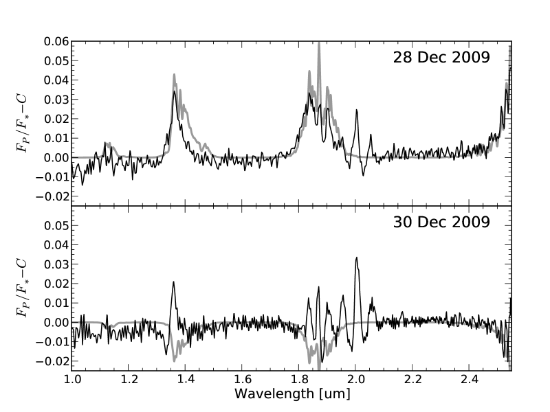
Figure 10.— width=3.5in

The effect of changes in telluric water absorption during our observations. The thin black line shows the measured residual eclipse spectrum, while the thick gray line represents the apparent eclipse signal ($\Delta\textrm{Tran}$) that would be inferred from the uncorrected changes in telluric PWV shown in Fig. LABEL:fig:tau. The 28 Dec spectrum appears strongly correlated with the $\Delta\textrm{Tran}$ signal, but the 30 Dec spectrum does not. Neither $\Delta\textrm{Tran}$ spectrum is significant far from telluric water absorption lines.

For both nights, the $\Delta\textrm{Tran}$ spectra do not capture the large spectral variations in the eclipse spectra from $2-2.07$ µm where there are strong telluric $\textrm{CO}_{2}$ absorption bands. We generate several ATRAN atmospheric profiles with varying concentrations of $\textrm{CO}_{2}$ but find that the in- and out-of-eclipse $\textrm{CO}_{2}$ concentrations must differ by $>5$ ppm to reproduce the features seen at these wavelengths. Such a change would be greater than any hour-to-hour change recorded at Mauna Loa by the National Oceanic and Atmospheric Administration Earth System Research Laboratory (NOAA ESRL) during all of 2009 (Thoning et al., 2010). Thus the telluric residuals in this wavelength range, though clearly correlated with the telluric $\textrm{CO}_{2}$ bands, are more likely attributable to the non-logarithmic relationship between flux and airmass in near-saturating lines and not to time-variable concentration.

As noted, $\Delta\textrm{Rad}$ is negligible across most of our passband, reaching $<2\times 10^{-4}$ by 2.4 µm for our PWV values. The magnitude of $\Delta\textrm{Tran}$ shown in Fig. LABEL:fig:pwv_effects is $<2\times 10^{-4}$ for our observations in the wavelength ranges $1-1.1$ µm, $1.22-1.30$ µm, $1.52-1.72$ µm, and $2.03-2.34$ µm. We further exclude the spectral regions affected by $\textrm{CO}_{2}$ ($2.00-2.08$ µm). So long as we restrict our analysis to these regions we consider it unlikely that telluric water or $\textrm{CO}_{2}$ significantly affect our results on either night.

Methane is another species whose abundance we are interested in measuring but whose telluric concentration can vary on short timescales. The NOAA ESRL also measures atmospheric $\textrm{CH}_{4}$ content (Dlugokencky et al., 2011), so we examined the hourly logs. The largest hour-to-hour change during our observations was $\sim 0.5\,\%$, with typical hourly changes smaller by a factor of several. We again use ATRAN (Lord, 1992) to simulate two atmospheric transmission spectra with methane amounts varying by 0.5 % (PWV was set to 1 mm and we simulated observations at zenith), and we then calculate $\Delta\textrm{Tran}$ as before. At our spectral resolution we find that $\Delta\textrm{Tran}$ reaches a maximum of about 0.04 % near 2.36 µm and is $<10^{-4}$ outside of $2.23-2.4\,\micron$. We include this $\Delta\textrm{Tran}$ spectrum as a wavelength-dependent systematic uncertainty in our final measurements.

5.2. Chromatic Slit Losses

We quantify the impact of chromatic slit loss on our data by modeling this effect and then trying to extract spectroscopic information from the simulation. For this modeling we use an implementation based on lightloss.pro in the SpeXTool (Cushing et al., 2004) distribution; this in turn is based on the discussion of atmospheric dispersion in Green (1985; their Eq. 4.31). A crucial factor in these simulations is the refractive index of air, which we model following Boensch & Potulski (1998) assuming air temperature, pressure, and composition that are constant but otherwise consistent with values typical for Mauna Kea. We also used our empirical measurements of the wavelength-dependent seeing FWHM and the positions of the spectra along the slit. We cannot measure atmospheric dispersion perpendicular to the slit’s long axis, so we calculate this wavelength-dependent quantity and then shift it by the spectral offsets measured in Sec. 2.2.

The result is a model of our chromatic slit loss which is based almost wholly on empirical data. We see some agreement between this model and our spectrophotometric throughput – e.g., less flux and chromatic tilt of the spectrum during brief periods of poor seeing. Though our modeling can qualitatively reproduce the types of variations seen, in detail the data are highly resistant to accurate modeling and we suspect additional dispersion and/or optical misalignments in SpeX may be to blame.

We suspect that our modeling is also limited by an imperfect knowledge of the (variable) instrument point spread function: the slit loss is most dependent on the distribution of energy along the dispersion direction, but we can only measure this shape perpendicular to the dispersion direction. We see 10% variations in the seeing from one frame to the next (as measured by the standard deviation of the frame-to-frame change in seeing FWHM) – whether this represents our fundamental measurement precision or the level of fluctuations in the instrument response, this level of variation prevents accurate and precise modeling of the chromatic slit loss.

Whatever the cause of the disagreement, our model appears qualitatively similar to the spectrophotometric variations apparent in our observations. We therefore proceed to extract a planetary spectrum after removing an achromatic slit loss term as described in Sec. 3.2. Although we input no planetary signal the spectrum extracted is nonzero because, in general, the projection of the achromatic slit loss vector onto the model eclipse light curve is nonzero. As the chromatic slit losses become more severe at shorter wavelengths, so too is the extracted planetary signal progressively more biased in those same regions. We then perform a pseudo-bootstrap analysis of the chromatic slit loss: we re-order the modeled slit transmission series – i.e., we move the first frame’s modeled slit transmission to the end of the data set and re-fit, then move the second frame’s transmission to the end, and repeat – and each time extract a planetary spectrum.

The variations in the extracted spectrum represent a systematic bias introduced by our wavelength-dependent slit losses. As expected observations taken with a wider slit fare better: for the 30 Dec observations the apparent variations in planetary emission (as measured by the standard deviation in each wavelength channel) are low in the H and K bands, reaching $\gtrsim 0.1\,\%$ (the approximate magnitude of the expected signal) in J band and rising shortward. However, our model of the 28 Dec observations indicates a substantially higher level of systematics: still low in the K band (where atmospheric dispersion is lessened; this is also our guiding wavelength, so variations are low here) but rising steeply with decreasing wavelength, reaching $\sim 0.5\,\%$ by the H band. We apply these noise spectra to our final measurement uncertainties to account for the possibility of systematic bias.

We also find that the induced spectral variations tend to depend more on changes in seeing than on atmospheric dispersion when using a 3.0” slit. This result suggests that our 30 Dec observations were not significantly compromised by our decision to lock down the instrument rotator.

5.3. Result of Simulated Observations

For completeness, we also combine our two dominant sources of systematic uncertainties – telluric absorption and chromatic slit loss effects – in a comprehensive model of our observations, using all empirical data available to us. We use a stellar template for the star (Castelli & Kurucz, 2004) and inject a model planetary spectrum (Madhusudhan et al., 2011, the purple curve in their Fig. 1, in which temperature decreases monotonically with decreasing pressure and with the largest predicted 2.36 µm $\textrm{CH}_{4}$ bandhead) and modulated by an analytical eclipse light curve (Hebb et al., 2009). For each frame we simulate the telluric transmission for each observation with LBLRTM (Clough et al., 2005), using the appropriate zenith angle and atmospheric water content (determined by interpolating the CSO observations in Sec. 5.1 to the time of the observation). We model the chromatic slit loss as described in the previous section and do not introduce any measurement noise into these simulated observations; this is because our goal is only to investigate the systematic biases the aforementioned effects have on our spectral extraction procedures. We also assume the detector response and instrumental throughput (excluding slit losses) are constant in time and wavelength. Any temporal variations in detector sensitivity will manifest themselves as increased scatter in the residuals and thus propagate to larger uncertainties in the prayer-bead analysis.

After generating these simulated spectra, we then send them through the analysis pipeline described in Sec. 4. We plot the extracted planetary spectra in Fig. LABEL:fig:simulation. As expected, our analysis performs poorly in regions of strong telluric absorption due to a combination of changing abundances and the more complicated behavior of partially saturated absorption lines; the telluric-induced errors are qualitatively similar to those seen in our simpler analysis of Sec. 5.1, confirming our decision to avoid these wavelengths.

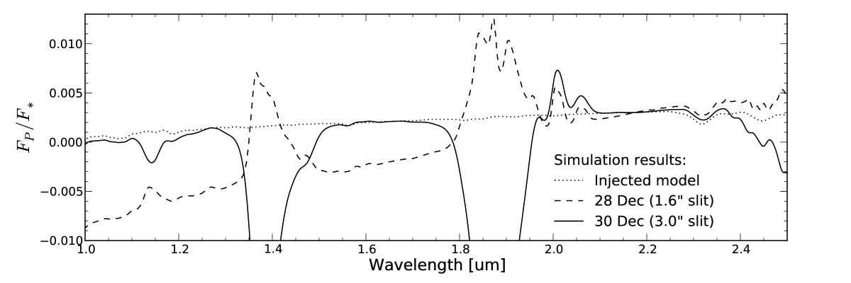
Figure 11.— width=3.5in

Planetary spectra extracted from our simulated observations; the difference between these and the injected model (from Madhusudhan et al., 2011) demonstrates the systematic biases present in our data. Changes in telluric water content introduce biases in particular spectral regions, while chromatic slit losses introduce gradients across all wavelengths, especially with a narrow slit and/or at short wavelengths. See Sec. 5.3 for a complete description.

Fig. LABEL:fig:simulation also demonstrates the large systematic bias introduced by chromatic slit losses. The effect is especially pronounced at short wavelengths and, in the case of the narrower (1.6”) slit, the bias is so large as to prevent this data set from setting any useful constraints on WASP-12b’s emission. This finding agrees with our estimate of the systematic uncertainties induced by chromatic slit losses in the previous section.

Having developed at least a rough understanding of our data’s expected biases, we are now well-equipped to interpret the results of our spectroscopic analysis.

6. Results: Thermal Emission from WASP-12b

6.1. Initial Presentation of Results

The parameters $d^{\lambda}$ that result from the fitting process represent a modified emission spectrum of WASP-12b, specifically $d^{\lambda}=F_{P}^{\lambda}/F_{*}^{\lambda}-C$. The constant $C$ results from our correction for common-mode photometric variations, and we set it using photometric eclipse measurements as described in Sec. 6. The individual channel (i.e., unbinned) best-fit coefficients for 28 Dec and 30 Dec are plotted in Figs. LABEL:fig:dec28_fitcoefs and LABEL:fig:dec30_fitcoefs, respectively, and we show the fit residuals in Fig. 12. We plot the binned eclipse spectra and their uncertainties (the quadrature sum of statistical and systematic errors) in Fig. 13.

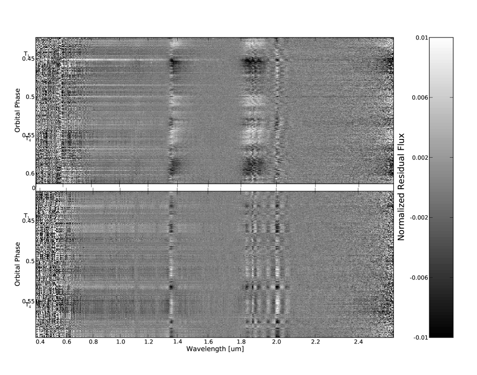
Figure 12.— Residuals to the data for the nights of 28 Dec (top) and 30 Dec (bottom) after fitting Eq. 1 to the data in each wavelength channel, normalized by the median flux value in each wavelength channel. Residual correlated errors remain at shorter wavelengths and in regions of strong telluric absorption. The first ($T_{1}$) and fourth ($T_{4}$) points of contact of the eclipse are noted, as calculated from the ephemeris of Hebb et al. (2009).

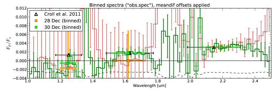
Figure 13.— Emission spectra (solid lines, binned to squares) after calibrating our relative measurement with the absolute photometry of Croll et al. (2011) (black triangles). The 28 Dec observations (red) suffer from extremely large systematic uncertainties at shorter wavelengths (cf. Fig. LABEL:fig:simulation), and uncertainties are also large in the J band for the 30 Dec observations (green). The K$-$H color we measure on 30 Dec agrees with the previous photometric value. The dashed line at bottom shows the observed telluric extinction coefficient.

Our measurement errors generally increase toward shorter wavelengths owing to the systematic biases discussed in Sec. 5.2. Our performance also worsens in regions of high telluric absorption; this is either because our simple modeling does not accurately capture the behavior of saturating absorption lines, or because the abundances of the absorbing telluric species are changing with time. As we describe in Sec. 5.1 above we believe the latter description applies to the behavior of the 28 Dec eclipse spectrum in water absorption bands, while the former applies to the strong $\textrm{CO}_{2}$ absorption bands (around $2-2.07$ µm) on both nights.

As expected from Secs. 5.2 and 5.3 and Fig. LABEL:fig:simulation, the large uncertainties for the 28 Dec data (deriving from our use of a narrow slit and our decision not to guide along the parallactic angle) prevent the 28 Dec data from usefully constraining WASP-12b’s emission. In our final analysis we thus use only the wide-slit (30 Dec) data, which our modeling suggests are the most reliable.

6.2. Comparison With Observations

As we have noted throughout, we make only a relative eclipse measurement because division by the slit loss term removes a mean eclipse signature from all channels. Precise photometric eclipse measurements (Croll et al., 2011) allow us to tie our observations to an absolute scale. From our investigation of systematic effects in Sec. 5.1 we expect our measurements to be robust in telluric-free regions of the H and K bands, but we expect systematics to limit our precision at shorter wavelengths and in any region of strong telluric absorption.

The H and Ks filters used by Croll et al. (2011) cover part of the telluric absorption band from $1.78-1.98$ µm, and without an independent calibration source we strongly mistrust our extracted spectra in these regions. We average our spectra over wavelength ranges corresponding approximately to the CFHT/WIRCam filter responses, but modified as necessary to avoid strong telluric features where our analysis is compromised: we use ranges of $1.52-1.72$ µm and $2.08-2.31$ µm to correspond to the H and K bands, respectively. The regions we avoid have greater telluric absorption, so these wavelengths contribute relatively less to the photometric measurements. Though telluric contamination thus precludes a truly homogeneous comparison between our results and those of Croll et al. (2011), using a blackbody model we estimate that the different wavelength ranges results in a difference of only 0.01 %, well beneath the precision we demonstrate below.

We compute K$-$H contrast colors (i.e., differential eclipse depths) on 28 Dec and 30 Dec of $0.31\,\%\pm 0.69\,\%$ and $0.137\,\%\pm 0.054\,\%$, respectively. The former value has a much larger uncertainty for the reasons discussed above in Sec. 5.3: the 28 Dec observations used a narrow (1.6”) slit and so are much more susceptible to systematic errors. We thus discard the 28 Dec spectrum and adopt the 30 Dec spectrum as our best estimate of WASP-12b’s emission. We thus have a K$-$H contrast color ($0.137\,\%\pm 0.054\,\%$) fully consistent with, though of a lower precision than, the photometric value of $0.133\%\pm 0.022$ % (Croll et al., 2011). WASP-12b’s broadband NIR emission closely approximates that of a 3,000 K blackbody (Croll et al., 2011; Madhusudhan et al., 2011); our contrast color is consistent with a blackbody of temperature $2400^{+1500}_{-500}~{}\textrm{K}$, confirming this result. The 30 Dec K$-$J contrast color is $0.36\,\%\pm 0.14\,\%$, which is also consistent with the photometric value of $0.178\%\pm 0.031\%$ (Croll et al., 2011) but is more uncertain: this large uncertainty exists because chromatic slit losses could substantially bias our measurement at these shorter wavelengths even with a 3.0” slit. Since the J-band uncertainties are dominated by the seeing-dependent component of chromatic slit losses, it may be difficult to improve on the short-wavelength performance we demonstrate here.

The weighted mean difference between our H and K measurements and those of Croll et al. (2011) is $0.236\,\%\pm 0.029\,\%$, consistent with the offset of 0.215 % expected from spectral models (Madhusudhan et al., 2011) given the wavelengths used in our initial correction with the achromatic slit loss time series. We adjust our relative spectra by this offset and thus place our measurements on an absolute scale. The calibrated spectra from each individual night are plotted in Fig. 13 and we show our final planet/star contrast spectrum, plotted over the wavelengths we consider to be uncorrupted by telluric effects, in Fig. 14 and list the contrast ratios in each wavelength bin in Table 2.

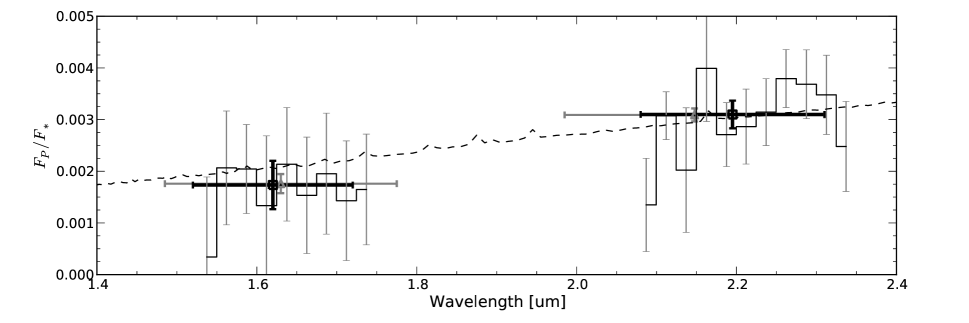
Figure 14.— Tentative planet/star contrast spectrum of the WASP-12 system from our 30 Dec observations. We have calibrated our relative spectroscopic measurements (thin black curve, binned to thick black squares) with photometric data points (gray triangles; Croll et al., 2011). Horizontal errorbars represent the effective widths of the photometric bandpasses; the ranges differ to prevent telluric variations from corrupting our single-slit observations. The dashed line shows the flux expected from a 3,000 K blackbody divided by the stellar flux model described in Sec. 6.4. Systematic uncertainties are larger at shorter wavelengths due to chromatic slit losses, so we do not plot those data here.

Table 2 Calibrated Planet/Star Contrast Spectrum

Wavelength Range (µm)	$F_{P}/F_{*}$ ($10^{-3}$)
$1.525-1.550$	0.34 $\pm$ 1.55
$1.550-1.575$	2.06 $\pm$ 1.10
$1.575-1.600$	2.04 $\pm$ 0.86
$1.600-1.625$	1.33 $\pm$ 1.35
$1.625-1.650$	2.13 $\pm$ 1.10
$1.650-1.675$	1.53 $\pm$ 1.13
$1.675-1.700$	1.95 $\pm$ 1.17
$1.700-1.725$	1.43 $\pm$ 1.16
$1.725-1.750$	1.65 $\pm$ 1.07
$2.075-2.100$	1.35 $\pm$ 0.90
$2.100-2.125$	3.08 $\pm$ 0.46
$2.125-2.150$	2.02 $\pm$ 1.21
$2.150-2.175$	3.99 $\pm$ 1.03
$2.175-2.200$	2.71 $\pm$ 0.62
$2.200-2.225$	2.86 $\pm$ 0.73
$2.225-2.250$	3.14 $\pm$ 0.65
$2.250-2.275$	3.79 $\pm$ 0.56
$2.275-2.300$	3.68 $\pm$ 0.67
$2.300-2.325$	3.48 $\pm$ 0.77
$2.325-2.350$	2.48 $\pm$ 0.87

6.3. Spectral Signatures: Still Unconstrained

The most prominent spectral signature predicted to lie in our spectral range is the 2.32 µm $\textrm{CH}_{4}$ absorption bandhead (Madhusudhan et al., 2011). We consider the model from Madhusudhan et al. (2011) in which temperature decreases monotonically with decreasing pressure (the purple curve in their Fig. 1), which is the model with the largest predicted $\textrm{CH}_{4}$ bandhead equivalent width. Estimating the continuum using wavelengths from $2.1\,\micron-2.25\,\micron$ and measuring the equivalent width from $2.25\,\micron-2.34\,\micron$, we calculate this feature’s equivalent width (calculated as a planet/star contrast) to be 16 nm in the model; with our spectrum we can set a 3$\sigma$ upper limit of $27~{}\textrm{nm}$.

We therefore come within a factor of two of being able to measure the strength of a specific spectral feature, and thus of spectroscopically constraining atmospheric abundances. However, because the uncertainties at these wavelengths are dominated by systematics relating to telluric absorption (cf. Sec. 5.1), a convincing detection would require many eclipses and a more complete understanding of the effects of telluric methane absorption.

6.4. Global Planetary Energy Budget

In light of our confirmation that WASP-12b’s NIR contrast color matches that of a 3,000 K blackbody, we revisit the published eclipse depths for WASP-12b with an eye toward examining the planet’s global energy budget. Since the orbital eccentricity is consistent with zero (Campo et al., 2011; Husnoo et al., 2011) we neglect tidal effects as a possible energy source and focus only on reprocessed stellar energy.

We convert eclipse depths (López-Morales et al., 2010; Croll et al., 2011; Campo et al., 2011) into surface fluxes using the known system parameters (Hebb et al., 2009), propagating the uncertainties in these parameters throughout our subsequent analysis. We use Castelli & Kurucz (2004) models with $T_{eff}=6250$ and 6500 K, $\log g=4.0$ and  4.5 (cgs units), and [M/H]$=+0.2$ and $+0.5$, and interpolate linearly in each of these quantities to the WASP-12 parameters of 6300 K, 4.16, and 0.3. Using the known WASP-12 system parameters we then convert to planetary fluxes using appropriate filter transmission profiles in each waveband (z’, J, H, and Ks from the ground, and all four IRAC channels on the Spitzer Space Telescope). In the same manner we convert our contrast ratio spectrum in Fig. 14 into a surface flux spectrum. We plot the full set of flux-calibrated eclipse measurements for this system in Fig. 15.

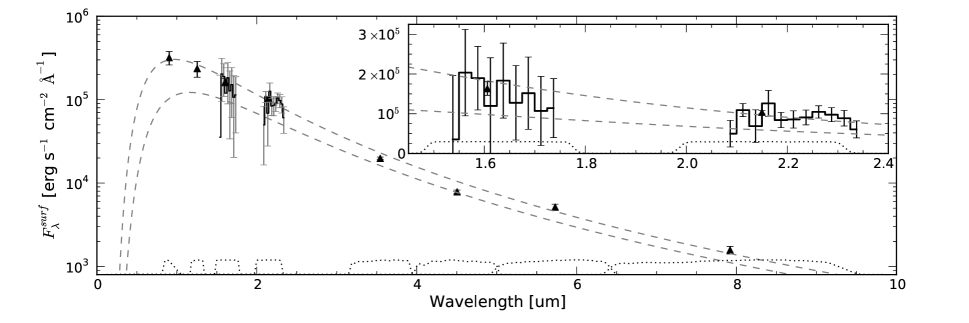
Figure 15.— Flux-calibrated spectral energy distribution of WASP-12b. Triangles are from previous optical (López-Morales et al., 2010), NIR (Croll et al., 2011), and mid-infrared (Campo et al., 2011) photometry, and the solid line (magnified in the inset) shows our measurements. The dashed lines show the surface flux of blackbodies with temperatures of 3,000 K and 2,500 K. The dotted lines at bottom show the filter transmission profiles described in Sec. 6.4.

We use the filter profiles and WASP-12b’s known size to then compute the dayside luminosity density. The current set of measurements puts a lower limit on the dayside luminosity of $2.0\times 10^{30}$ erg s^-1. This value is a lower limit because it assumes zero flux outside the filter bandpasses, which is improbable. Modeling the planet’s spectrum between filters as a piecewise linear function increases the measured luminosity to $3.6\times 10^{30}$ erg s^-1. As noted previously, the planet’s broadband spectrum closely approximates a 3,000 K blackbody (Madhusudhan et al., 2011); such a spectrum would emit an additional $0.7\times 10^{30}$ erg s^-1 shortward of the z’ band. The presence of any optical absorbers (as has been observed on some planets: e.g., Charbonneau et al., 2002; Sing et al., 2011) would tend to decrease this optical emission. We thus estimate the planet’s total dayside luminosity to lie in the range $(2.0-4.3)\times 10^{30}$ erg s^-1.

On the other hand, WASP-12b absorbs $(1-A_{B})(5.1\pm 0.8)\times 10^{30}$ erg s^-1 of stellar energy, where $A_{B}$ is the planet’s Bond albedo. Cowan & Agol (2011b) have suggested that the hottest of the Hot Jupiters (including the 3,000 K WASP-12b) have low albedos and low energy recirculation efficiencies; assuming zero albedo, our calculations limit the nightside luminosity to $(0.8-3.1)\times 10^{30}$ erg s^-1.

Approximating the nightside as a blackbody of uniform temperature, these values correspond to a nightside effective temperature of 2,000$-$2,800 K or a day-night effective temperature contrast of $200-$1,000 K. Temperature contrasts of this magnitude would correspond to a planetary energy recirculation efficiency (Cowan & Agol, 2011a) of $\epsilon=2-10$, which suggests that the planet’s recirculation efficiency may not be as low as predicted if the planet also has a low albedo (cf. Cowan & Agol, 2011b). This result should be relatively easy to test, since these temperature contrasts imply IRAC1 & 2 phase curve contrasts ($\Delta F/\langle F\rangle$, cf. Cowan et al., 2007) of as much as $0.25$ % and a Ks-band phase curve contrast of $\lesssim$ 0.15 %. Warm Spitzer can easily reach this precision, and the results will help constrain WASP-12b’s recirculation efficiency and Bond albedo. After referral of this manuscript we became aware of just such a set of IRAC observations (Cowan et al., 2011). Though of limited precision, these Spitzer observations support our predictions above and suggest that WASP-12b has a nonzero albedo and low recirculation efficiency.

Eclipse observations still do not bracket the flux peak of WASP-12b’s emission: $F_{\lambda}$ increases monotonically from 8 µm (IRAC4) to 0.9 µm (z’ band). We therefore strongly encourage efforts to detect the planet’s emission and/or reflection at shorter wavelengths (e.g., in the I and R bands) to further refine the planet’s albedo and flesh out its energy budget. The optical planet/star contrast ratios are challenging ($<0.08$ %) but should be attainable on modest-sized (3-4 m) ground-based telescopes or with the Hubble Space Telescope (HST). HST observations at wavelengths inaccessible from the ground would also help fill the gaps in the planet’s spectral energy distribution and so decrease the uncertainty in the planet’s dayside luminosity.

7. Lessons for Future Observations

Our primary, but ultimately tentative result is WASP-12b’s K$-$H contrast color of $0.137\,\%\pm 0.054\,\%$. This result is a factor of 2.5 less precise than that determined by wide-field, relative eclipse photometry (Croll et al., 2011) with a comparable amount of observing time. Nonetheless, we are heartened by our ability to self-calibrate out correlated noise in pursuit of precise relative measurement and to come within a factor of two of constraining the strengths of specific molecular features. This suggests that many repeated observations with SpeX or similar wide-slit spectrograph might descry spectral signatures. However, more progress must be demonstrated for single-slit observations to be competitive with photometry. The field is only now developing the beginnings of an understanding of telluric effects on such observations (Mandell et al., 2011), and there is still no consensus explanation for the full set of observations of Swain et al. (2010).

Our analysis in Sec. 5 demonstrates that telluric variations can imprint spurious features on our planetary spectrum, and chromatic slit losses can induce broad spectral gradients. Certainly, future observations should guide the slit along the parallactic angle and use as large a slit as possible. Future SpeX observations should make use of MORIS (Gulbis et al., 2011), a camera allowing simultaneous NIR spectroscopy and optical imaging, to distinguish between telluric transparency effects and instrumental throughput variations coupled to variable seeing, pointing, and PSF morphology. It could be possible to improve future performance by modeling the evolution of telluric features using high-resolution spectra, but we suspect this will not be feasible for very low-resolution observations such as those presented here. In any event, we would prefer to eschew telluric modeling and the many additional complications such analyses must entail. At this point we cannot say whether the increase in throughput afforded by prism mode was worth the cost in lower resolution, but we have SpeX echelle data in hand (and more pending) that may allow us to answer this question. In any case higher resolution will not substantially improve the resolution of our final planetary spectrum, because substantial binning is still required to achieve a useful S/N.

As we stated in Paper I, we believe that near-infrared, multi-object spectrographs (MOS) will be the key technology that will enable detailed spectroscopic studies of exoplanet atmospheres. As the high precision achieved with optical and NIR MOS units (Bean et al., 2010, 2011) demonstrates, these instruments may well prove transformative for such studies. Slits can be made large enough to avoid all pointing error-induced slit loss effects, and simultaneous spectra of multiple calibrator stars allow all the advantages enjoyed by relative photometric techniques to be transferred to the field of spectroscopy. The spectroscopic calibrator stars provided by a MOS largely eliminates spectral contamination due to changes in telluric water transmission (i.e., $\Delta\textrm{Tran}$) since the calibrator observations remove telluric transmission effects in the same manner as is done in relative transit photometry. This should largely obviate the need to model evolving airmass extinction effects. Because the large majority of multi-object spectrographs work at wavelengths where $\Delta\textrm{Rad}$ effects are negligible, with multi-object observations neither telluric radiance nor transmittance should prove a confounding factor.

However, a large fraction of the currently known transiting systems will remain off-limits to the multi-object technique. This can result either from systems which lack comparison stars of adequate brightness within several arc minutes of the exoplanet host star, or from host stars that are too bright to observe with the large-aperture telescopes currently hosting MOS units. Transiting planets in these systems can be observed spectroscopically at $\lambda<1.7\,\micron$ with Hubble/WFC3 (cf. Berta et al., 2011), but spectroscopy in the K and L bands (where $\textrm{CH}_{4}$ and CO bands are prominent) will remain the domain of ground-based, single-slit spectroscopy for the near future.

Whatever the observing technique used, we emphasize the importance of observing multiple transit or eclipse events with ground-based observations. There are many subtle confounding factors in such analyses, and repeated observations are essential to discriminate between intermittent systematic effects and a true planetary signal. Many nights of observations would be required with SpeX to build up a useful spectroscopic S/N for most systems, but it does seem feasible. Nonetheless even with large-aperture telescopes single-epoch observations – including the results we present here – may well be treated with some skepticism.

8. Conclusions

We have presented evidence for a tentative spectroscopic detection of near-infrared emission from the extremely Hot Jupiter WASP-12b. Our data are compromised by correlated noise: spectrophotometric variations induced by telluric variations (owing to changing airmass and telluric abundances) and instrumental instabilities (caused mainly by fluctuations in the instrument PSF, but also by atmospheric dispersion) that are largely, but not wholly, common-mode across our wavelength range. By removing a common time series from all our data we self-calibrate and remove much of this variability, but biases remain. Though this calibration subtracts an unknown constant offset from our measured spectrum we renormalize using contemporaneous eclipse photometry (Croll et al., 2011).

Although we present a possible emission spectrum of the planet in Fig. 14, uncertainties are still too large (by a factor of two) to constrain the existence of putative $\textrm{CH}_{4}$ absorption features. We measure a K$-$H contrast color of $0.137\,\%\pm 0.054\,\%$, consistent with a blackbody of temperature $2400^{+1500}_{-500}~{}\textrm{K}$; thus our results agree with (but are less precise than) previous photometric observations (Croll et al., 2011). Our spectroscopic precision is limited by residual correlated noise and, due to our lack of external calibrators, by our extreme susceptibility to interference from telluric and instrumental sources outside a fairly narrow wavelength range. Modeling (described in Sec. 5) gives us confidence that within these regions our planetary spectrum is free of telluric contamination and (with a 3.0” slit) chromatic slit losses play a negligible role at $\lambda>1.4\,\micron$.

Our primary result is methodological: to avoid biases from chromatic slit losses single-slit, NIR spectroscopy of transiting exoplanets should use slits as wide as possible and always keep the slit aligned to the parallactic angle. Instruments must be kept well-focused throughout such observations to minimize the effects of seeing variations. Substantially more attention must be paid to telluric variations if observations are to extend beyond the fairly narrow windows we describe in Sec. 5.1.

We predict that multi-object spectrographs will easily achieve better performance than what we have demonstrated here: wider slits and multiple simultaneous calibration stars will measure and remove instrumental and telluric systematics. These instruments are deployed on an ever-growing number of large-aperture telescopes and are beginning to be put to the test. In the meantime, we hope our descriptions of these first stumbling efforts will inform future studies so that the routine, detailed characterization of exoatmospheres can begin in earnest.

References

- Andrae (2010) Andrae, R. 2010, ArXiv e-prints, ADS, 1009.2755
- Barnes et al. (2007) Barnes, J. R., Leigh, C. J., Jones, H. R. A., Barman, T. S., Pinfield, D. J., Collier Cameron, A., & Jenkins, J. S. 2007, MNRAS, 379, 1097, ADS, 0705.0272
- Bean et al. (2011) Bean, J. L. et al. 2011, ArXiv e-prints, ADS, 1109.0582
- Bean et al. (2010) Bean, J. L., Miller-Ricci Kempton, E., & Homeier, D. 2010, Nature, 468, 669, ADS, 1012.0331
- Berta et al. (2011) Berta, Z. K. et al. 2011, ArXiv e-prints, ADS, 1111.5621
- Boensch & Potulski (1998) Boensch, G., & Potulski, E. 1998, Metrologia, 35, 133
- Brown et al. (2002) Brown, T. M., Libbrecht, K. G., & Charbonneau, D. 2002, PASP, 114, 826, ADS, arXiv:astro-ph/0205246
- Campo et al. (2011) Campo, C. J. et al. 2011, ApJ, 727, 125, ADS, 1003.2763
- Castelli & Kurucz (2004) Castelli, F., & Kurucz, R. L. 2004, ArXiv Astrophysics e-prints, ADS, arXiv:astro-ph/0405087
- Chan et al. (2011) Chan, T., Ingemyr, M., Winn, J. N., Holman, M. J., Sanchis-Ojeda, R., Esquerdo, G., & Everett, M. 2011, AJ, 141, 179, ADS, 1103.3078
- Charbonneau et al. (2002) Charbonneau, D., Brown, T. M., Noyes, R. W., & Gilliland, R. L. 2002, ApJ, 568, 377, ADS, arXiv:astro-ph/0111544
- Clough et al. (2005) Clough, S., Shephard, M., Mlawer, E., Delamere, J., Iacono, M., Cady-Pereira, K., Boukabara, S., & Brown, P. 2005, Journal of Quantitative Spectroscopy and Radiative Transfer, 91, 233 , ADS
- Cowan & Agol (2011a) Cowan, N. B., & Agol, E. 2011a, ApJ, 726, 82, ADS, 1011.0428
- Cowan & Agol (2011b) —. 2011b, ApJ, 729, 54, ADS, 1001.0012
- Cowan et al. (2007) Cowan, N. B., Agol, E., & Charbonneau, D. 2007, MNRAS, 379, 641, ADS, 0705.1189
- Cowan et al. (2011) Cowan, N. B., Machalek, P., Croll, B., Shekhtman, L. M., Burrows, A., Deming, D., Greene, T., & Hora, J. L. 2011, ArXiv e-prints, ADS, 1112.0574
- Croll et al. (2011) Croll, B., Lafreniere, D., Albert, L., Jayawardhana, R., Fortney, J. J., & Murray, N. 2011, AJ, 141, 30, ADS, 1009.0071
- Crossfield et al. (2011) Crossfield, I. J. M., Barman, T., & Hansen, B. M. S. 2011, ApJ, 736, 132, ADS, 1104.1173
- Cushing et al. (2004) Cushing, M. C., Vacca, W. D., & Rayner, J. T. 2004, PASP, 116, 362, ADS
- Deming et al. (2005) Deming, D., Brown, T. M., Charbonneau, D., Harrington, J., & Richardson, L. J. 2005, ApJ, 622, 1149, ADS, arXiv:astro-ph/0412436
- Deroo et al. (2010) Deroo, P., Swain, M. R., & Vasisht, G. 2010, ArXiv e-prints, ADS, 1011.0476
- Dlugokencky et al. (2011) Dlugokencky, E. J., Lang, P. M., & Masarie, K. A. 2011, Methane Dry Air Mole Fractions from quasi-continuous measurements at Barrow, Alaska and Mauna Loa, Hawaii, 1986-2010, ftp://ftp.cmdl.noaa.gov/ccg/ch4/in-situ/
- Filippenko (1982) Filippenko, A. V. 1982, PASP, 94, 715, ADS
- Fortney et al. (2007) Fortney, J. J., Marley, M. S., & Barnes, J. W. 2007, ApJ, 659, 1661, arXiv:astro-ph/0612671
- Gibson et al. (2011) Gibson, N. P., Pont, F., & Aigrain, S. 2011, MNRAS, 411, 2199, ADS, 1010.1753
- Gillon et al. (2007) Gillon, M. et al. 2007, A&A, 471, L51, ADS, 0707.2261
- Green (1985) Green, R. M. 1985, Spherical astronomy, ed. Green, R. M., ADS
- Gulbis et al. (2011) Gulbis, A. A. S. et al. 2011, PASP, 123, 461, ADS, 1102.5248
- Hebb et al. (2009) Hebb, L. et al. 2009, ApJ, 693, 1920, ADS
- Hinkle et al. (2003) Hinkle, K. H., Wallace, L., & Livingston, W. 2003, 35, 1260, ADS
- Husnoo et al. (2011) Husnoo, N. et al. 2011, MNRAS, 413, 2500, ADS, 1004.1809
- Knutson et al. (2007) Knutson, H. A., Charbonneau, D., Deming, D., & Richardson, L. J. 2007, PASP, 119, 616, 0705.4288
- Knutson et al. (2010) Knutson, H. A., Howard, A. W., & Isaacson, H. 2010, ApJ, 720, 1569, ADS, 1004.2702
- Li et al. (2010) Li, S.-L., Miller, N., Lin, D. N. C., & Fortney, J. J. 2010, Nature, 463, 1054, ADS, 1002.4608
- López-Morales et al. (2010) López-Morales, M., Coughlin, J. L., Sing, D. K., Burrows, A., Apai, D., Rogers, J. C., Spiegel, D. S., & Adams, E. R. 2010, ApJ, 716, L36, ADS, 0912.2359
- Lord (1992) Lord, S. D. 1992, A new software tool for computing Earth’s atmospheric transmission of near- and far-infrared radiation, Tech. rep., ADS
- Madhusudhan et al. (2011) Madhusudhan, N. et al. 2011, Nature, 469, 64, ADS, 1012.1603
- Madhusudhan & Seager (2010) Madhusudhan, N., & Seager, S. 2010, ApJ, 725, 261, ADS, 1010.4585
- Mandel & Agol (2002) Mandel, K., & Agol, E. 2002, ApJ, 580, L171, ADS
- Mandell et al. (2011) Mandell, A. M., Drake Deming, L., Blake, G. A., Knutson, H. A., Mumma, M. J., Villanueva, G. L., & Salyk, C. 2011, ApJ, 728, 18, ADS, 1011.5507
- Quirrenbach (2000) Quirrenbach, A. 2000, in Principles of Long Baseline Stellar Interferometry, ed. P. R. Lawson, 71–+, ADS
- Rayner et al. (2003) Rayner, J. T., Toomey, D. W., Onaka, P. M., Denault, A. J., Stahlberger, W. E., Vacca, W. D., Cushing, M. C., & Wang, S. 2003, PASP, 115, 362, ADS
- Redfield et al. (2008) Redfield, S., Endl, M., Cochran, W. D., & Koesterke, L. 2008, ApJ, 673, L87, ADS, 0712.0761
- Richardson et al. (2003) Richardson, L. J., Deming, D., Wiedemann, G., Goukenleuque, C., Steyert, D., Harrington, J., & Esposito, L. W. 2003, ApJ, 584, 1053, ADS
- Sing et al. (2009) Sing, D. K., Désert, J., Lecavelier Des Etangs, A., Ballester, G. E., Vidal-Madjar, A., Parmentier, V., Hebrard, G., & Henry, G. W. 2009, A&A, 505, 891, ADS, 0907.4991
- Sing et al. (2011) Sing, D. K. et al. 2011, A&A, 527, A73+, ADS, 1008.4795
- Smith et al. (2001) Smith, G. J., Naylor, D. A., & Feldman, P. A. 2001, International Journal of Infrared and Millimeter Waves, 22, 661, 10.1023/A:1010689508585
- Snellen et al. (2008) Snellen, I. A. G., Albrecht, S., de Mooij, E. J. W., & Le Poole, R. S. 2008, A&A, 487, 357, ADS, 0805.0789
- Snellen et al. (2010) Snellen, I. A. G., de Kok, R. J., de Mooij, E. J. W., & Albrecht, S. 2010, Nature, 465, 1049, ADS, 1006.4364
- Swain et al. (2008) Swain, M. R., Bouwman, J., Akeson, R. L., Lawler, S., & Beichman, C. A. 2008, ApJ, 674, 482, arXiv:astro-ph/0702593
- Swain et al. (2010) Swain, M. R. et al. 2010, Nature, 463, 637, ADS, 1002.2453
- Thoning et al. (2010) Thoning, K. W., Kitzis, D. R., & Crotwell, A. 2010, Carbon Dioxide Dry Air Mole Fractions from quasi-continuous measurements at Barrow, Alaska; Mauna Loa, Hawaii; American Samoa; and South Pole, 1973-2009, ftp://ftp.cmdl.noaa.gov/ccg/co2/in-situ/
- Waldmann et al. (2011) Waldmann, I. P., Drossart, P., Tinetti, G., Griffith, C. A., Swain, M. R., & Deroo, P. 2011, ArXiv e-prints, ADS, 1104.0570