On the stability under convolution of
resurgent functions

Abstract

This article introduces, for any closed discrete subset $\Omega$ of $\mathbb{C}$, the definition of $\Omega$-continuability, a particular case of Écalle’s resurgence: $\Omega$-continuable functions are required to be holomorphic near $0$ and to admit analytic continuation along any path which avoids $\Omega$. We give a rigorous and self-contained treatment of the stability under convolution of this space of functions, showing that a necessary and sufficient condition is the stability of $\Omega$ under addition.

Keywords: Resurgent functions, convolution algebras. MSC: 30D05, 37F99.

1 Introduction

Écalle’s theory of resurgent functions is an efficient tool for dealing with divergent series arising from complex dynamical systems or WKB expansions, and for determining the analytic invariants of differential or difference equations. Fundamental notions of the theory are that of germs analytically continuable without a cut, and the related notion of endlessly continuable germs: these are holomorphic germs of one complex variable at the origin which enjoy a certain property of analytic continuation (the possible singularities of their analytic continuation must be isolated, at least locally—[Eca81], [Mal85], [CNP93]); they arise as Borel transforms of possibly divergent formal series which solve certain nonlinear problems.

Since the theory is designed to deal with nonlinear problems, it is an essential fact that the property of endless continuability (or of continuability without a cut) is stable under convolution (indeed, via Borel transform, the convolution of germs at $0$ reflects the Cauchy product of formal series). This allows to define the algebra of resurgent functions in the “convolutive model” and then to study certain subalgebras obtained by specifying the location or the nature of the possible singularities that one can encounter in the process of analytic continuation. Écalle then proceeds with defining the “alien calculus”, which involves particular derivations of this algebra and is an efficient way of encoding the singularities, and deriving consequences in the “geometric models” obtained by applying the Laplace transform in all possible directions; this is a way of describing nonlinear Stokes phenomena or of solving problems of analytic classification—see [Eca81], [Eca92], [Eca93], [CNP93], [Sau06], [Sau10], [Sau12].

Unfortunately, the proof of the stability under convolution of endlessly continuable germs in full generality is difficult. Écalle’s argument is based on the notion of “symmetrically contractile” paths, but the fact that one can always find such paths is a delicate matter. Therefore, when we came across a strikingly simple proof which applies to interesting subspaces of resurgent functions, we thought it was worthwhile to bring it to the attention of researchers interested in resurgence theory.

We shall deal in this article with a particular case of endless continuability, which we call $\Omega$-continuability, which corresponds to specifying a priori the possible location of the singularities: they are required to lie in a set $\Omega$ that we fix in advance. This means that there is one Riemann surface over $\mathbb{C}$, depending only on $\Omega$, on which every $\Omega$-continuable germ induces a holomorphic function (whereas in the general case of endless continuability there is an “endless” Riemann surface which does depend on the considered germ). This definition already covers interesting cases: one encounters $\Omega$-continuable germs with $\Omega=\mathbb{N}^{*}$ or $\Omega=\mathbb{Z}$ when dealing with differential equations formally conjugate to the Euler equation (in the study of the saddle-node singularities) [Eca84], [Sau10], or with $\Omega=2\pi{\mathrm{i}}\mathbb{Z}$ when dealing with certain difference equations like Abel’s equation for parabolic germs in holomorphic dynamics [Eca81], [Sau06], [DS12], [Sau12].

Our aim is to give a rigorous and self-contained treatment of the stability under convolution of the space of $\Omega$-continuable germs, with more details and more complete explanations than e.g. [Sau06] which was dealing with the particular case $\Omega=2\pi{\mathrm{i}}\mathbb{Z}$. For the latter case, the recent article [Ou10] is available, but our approach is different.

For any closed discrete subset of $\mathbb{C}$, we shall thus introduce the definition of $\Omega$-continuability in Section 2, recall the definition of convolution in Section 3 and state in Section 4 our main result, Theorem 4.1, which is the equivalence of the stability under convolution of $\Omega$-continuable germs and the stability under addition of the set $\Omega$. The rest of the article will be devoted to the proof of this theorem.

A novel feature of our proof (even if we certainly owe a debt to [Eca81] and [CNP93]) is the construction of “symmetric $\Omega$-homotopies” by means of certain non-autonomous vector fields.

2 The $\Omega$-continuable germs

In this article, “path” means a piecewise $C^{1}$ function $\gamma\colon\thinspace J\to\mathbb{C}$, where $J$ is a compact interval of $\mathbb{R}$. For any $R>0$ and ${\zeta}_{0}\in\mathbb{C}$ we use the notations $D({\zeta}_{0},R)\coloneqq\{\,{\zeta}\in\mathbb{C}\mid|{\zeta}-{\zeta}_{0}|<R\,\}$, $\mathbb{D}_{R}\coloneqq D(0,R)$ and $\mathbb{D}^{*}_{R}\coloneqq\mathbb{D}_{R}\setminus\{0\}$.

Definition 2.1.

Let $\Omega$ be a non-empty closed discrete subset of $\mathbb{C}$, let $\hat{\varphi}({\zeta})\in\mathbb{C}\{{\zeta}\}$ be a holomorphic germ at the origin. We say that $\hat{\varphi}$ is $\Omega$-continuable if there exists $R>0$ not larger than the radius of convergence of $\hat{\varphi}$ such that $\mathbb{D}^{*}_{R}\cap\Omega=\emptyset$ and $\hat{\varphi}$ admits analytic continuation along any path of $\mathbb{C}\setminus\Omega$ originating from any point of $\mathbb{D}^{*}_{R}$. We use the notation

$$\hat{\mathscr{R}}_{\Omega}\coloneqq\{\,\text{all $\Omega$-continuable holomorphic germs}\,\}\subset\mathbb{C}\{{\zeta}\}.$$

Remark 2.2.

Let $\rho\coloneqq\min\big{\{}|\omega|,\;\omega\in\Omega\setminus\{0\}\big{\}}$. Any $\hat{\varphi}\in\hat{\mathscr{R}}_{\Omega}$ is a holomorphic germ at $0$ with radius of convergence $\geq\rho$ and one can always take $R=\rho$ in Definition 2.1. In fact, given an arbitrary ${\zeta}_{0}\in\mathbb{D}_{\rho}$, we have

$$\hat{\varphi}\in\hat{\mathscr{R}}_{\Omega}\quad\Longleftrightarrow\quad\left|\begin{aligned} &\text{$\hat{\varphi}$ germ of holomorphic function of~{}$\mathbb{D}_{\rho}$ admitting analytic}\\ &\text{continuation along any path $\gamma\colon\thinspace[0,1]\to\mathbb{C}$ such that}\\ &\text{$\gamma(0)={\zeta}_{0}$ and $\gamma\big{(}(0,1]\big{)}\subset\mathbb{C}\setminus\Omega$}\end{aligned}\right.$$

(even if ${\zeta}_{0}=0$ and $0\in\Omega$: there is no need to avoid $0$ at the beginning of the path, when we still are in the disc of convergence of $\hat{\varphi}$).

Example 2.3.

Trivially, any entire function of $\mathbb{C}$ defines an $\Omega$-continuable germ. Other elementary examples of $\Omega$-continuable germs are the functions which are holomorphic in $\mathbb{C}\setminus\Omega$ and regular at $0$, like $\frac{1}{({\zeta}-\omega)^{m}}$ with $m\in\mathbb{N}^{*}$ and $\omega\in\Omega\setminus\{0\}$. But these are still single-valued examples, whereas the interest of the Definition 2.1 is to authorize multiple-valuedness when following the analytic continuation. Elementary examples of multiple-valued continuation are provided by $\sum_{n\geq 1}\frac{{\zeta}^{n}}{n}=-\log(1-{\zeta})$ (principal branch of the logarithm), which is $\Omega$-continuable if and only if $1\in\Omega$, and $\sum_{n\geq 0}\frac{{\zeta}^{n}}{n+1}=-\frac{1}{{\zeta}}\log(1-{\zeta})$, which is $\Omega$-continuable if and only if $\{0,1\}\subset\Omega$.

Example 2.4.

If $\omega\in\mathbb{C}^{*}$ and $m\in\mathbb{N}^{*}$, then $\big{(}\log({\zeta}-\omega)\big{)}^{m}\in\hat{\mathscr{R}}_{\{\omega\}}$; if moreover $\omega\neq-1$, then $\big{(}\log({\zeta}-\omega)\big{)}^{-m}\in\hat{\mathscr{R}}_{\{\omega,\omega+1\}}$.

Example 2.5.

If $\Omega$ is a closed discrete subset of $\mathbb{C}$, $0\notin\Omega$, $\omega\in\Omega$ and $\hat{\psi}$ is holomorphic in $\mathbb{C}\setminus\Omega$, then $\hat{\varphi}({\zeta})=\hat{\psi}({\zeta})\log({\zeta}-\omega)$ defines a germ of $\hat{\mathscr{R}}_{\Omega}$ whose monodromy around $\omega$ is given by $2\pi{\mathrm{i}}\hat{\psi}$.

Notation 2.6.

Given a path $\gamma\colon\thinspace[a,b]\to\mathbb{C}$, if $\hat{\varphi}$ is a holomorphic germ at $\gamma(a)$ which admits an analytic continuation along $\gamma$, we denote by $\operatorname{cont}_{\gamma}\hat{\varphi}$ the resulting holomorphic germ at the endpoint $\gamma(b)$.

As is often the case with analytic continuation and Cauchy integrals, the precise parametrisation of our paths will usually not matter, in the sense that we shall get the same results from two paths $\gamma\colon\thinspace[a,b]\to\mathbb{C}$ and $\gamma^{\prime}\colon\thinspace[a^{\prime},b^{\prime}]\to\mathbb{C}$ which only differ by a change of parametrisation ($\gamma=\gamma^{\prime}\circ{\sigma}$ with ${\sigma}\colon\thinspace[a,b]\to[a^{\prime},b^{\prime}]$ piecewise continuously differentiable, increasing and mapping $a$ to $a^{\prime}$ and $b$ to $b^{\prime}$).

We identify $\mathbb{C}\{{\zeta}\}$, the space of power series with positive radius of convergence, with the space of holomorphic germs at $0$. Given $\hat{\varphi}\in\mathbb{C}\{{\zeta}\}$, we shall often denote by the same symbol $\hat{\varphi}$ the holomorphic function it defines, or even the principal branch of its analytic continuation when such a notion is well-defined.

3 The convolution of holomorphic germs at the origin

The convolution in $\mathbb{C}\{{\zeta}\}$ is defined by the formula

$$\hat{\varphi}*\hat{\psi}({\zeta})\coloneqq\int_{0}^{\zeta}\hat{\varphi}(\xi)\hat{\psi}({\zeta}-\xi)\,{\mathrm{d}}\xi$$

for any $\hat{\varphi},\hat{\psi}\in\mathbb{C}\{{\zeta}\}$: the formula makes sense for $|{\zeta}|$ small enough and defines a holomorphic germ at $0$ whose disc of convergence contains the intersection of the discs of convergence of $\hat{\varphi}$ and $\hat{\psi}$. The convolution law $*$ is commutative and associative.

The question we address in this article is the question of the stability of $\hat{\mathscr{R}}_{\Omega}$ under convolution. As already mentioned, this is relevant when dealing with the formal solutions of nonlinear problems and this is absolutely necessary to develop the theory of resurgent functions and alien calculus for $\Omega$-continuable germs.

This amounts to inquiring about the analytic continuation of the germ $\hat{\varphi}*\hat{\psi}$ when $\Omega$-continuability is assumed for $\hat{\varphi}$ and $\hat{\psi}$. Let us first mention an easy case, which is used in [DS12] and [Sau10]:

Lemma 3.1.

Let $\Omega$ be any non-empty closed discrete subset of $\mathbb{C}$ and suppose $\hat{A}$ is an entire function of $\mathbb{C}$. Then, for any $\hat{\varphi}\in\hat{\mathscr{R}}_{\Omega}$, the convolution product $\hat{A}*\hat{\varphi}$ belongs to $\hat{\mathscr{R}}_{\Omega}$; its analytic continuation along a path $\gamma$ of $\mathbb{C}\setminus\Omega$ starting from a point ${\zeta}_{0}$ close enough to $0$ and ending at a point ${\zeta}_{1}$ is the holomorphic germ at ${\zeta}_{1}$ explicitly given by

$$\operatorname{cont}_{\gamma}(\hat{A}*\hat{\varphi})({\zeta})=\int_{0}^{{\zeta}_{0}}\hat{A}({\zeta}-\xi)\hat{\varphi}(\xi)\,{\mathrm{d}}\xi+\int_{\gamma}\hat{A}({\zeta}-\xi)\hat{\varphi}(\xi)\,{\mathrm{d}}\xi+\int_{{\zeta}_{1}}^{\zeta}\hat{A}({\zeta}-\xi)\hat{\varphi}(\xi)\,{\mathrm{d}}\xi$$ (1)

for ${\zeta}$ close enough to ${\zeta}_{1}$.

The proof is left as an exercise (see e.g. the proof of Lemma 5.3 for a formalized proof in a more complicated situation), but we wish to emphasize that formulas such as (1) require a word of caution: the value of $\hat{A}({\zeta}-\xi)$ is unambiguously defined whatever ${\zeta}$ and $\xi$ are, but in the notation “$\hat{\varphi}(\xi)$” it is understood that we are using the appropriate branch of the possibily multiple-valued function $\hat{\varphi}$; in such a formula, what branch we are using is clear from the context:

1. $\hat{\varphi}$ is unambiguously defined in its disc of convergence $D_{0}$ (centred at $0$) and the first integral thus makes sense for ${\zeta}_{0}\in D_{0}$;

2. in the second integral $\xi$ is moving along $\gamma$ which is a path of analytic continuation for $\hat{\varphi}$, we thus consider the analytic continuation of $\hat{\varphi}$ along the piece of $\gamma$ between its origin and $\xi$;

3. in the third integral, “$\hat{\varphi}$” is to be understood as $\operatorname{cont}_{\gamma}\hat{\varphi}$, the germ at ${\zeta}_{1}$ resulting form the analytic continuation of $\hat{\varphi}$ along $\gamma$, this integral then makes sense for any ${\zeta}$ at a distance from ${\zeta}_{1}$ less than the radius of convergence of $\operatorname{cont}_{\gamma}\hat{\varphi}$.

Using a parametrisation $\gamma\colon\thinspace[0,1]\to\mathbb{C}\setminus\Omega$, with $\gamma(0)={\zeta}_{0}$ and $\gamma(1)={\zeta}_{1}$, and introducing the truncated paths $\gamma_{s}\coloneqq\gamma_{|[0,s]}$ for any $s\in[0,1]$, the interpretation of the last two integrals in (1) is

$$\int_{\gamma}\hat{A}({\zeta}-\xi)\hat{\varphi}(\xi)\,{\mathrm{d}}\xi \coloneqq\int_{0}^{1}\hat{A}({\zeta}-\gamma(s))(\operatorname{cont}_{\gamma_{s}}\hat{\varphi})(\gamma(s))\gamma^{\prime}(s)\,{\mathrm{d}}s,$$

$$\int_{{\zeta}_{1}}^{\zeta}\hat{A}({\zeta}-\xi)\hat{\varphi}(\xi)\,{\mathrm{d}}\xi \coloneqq\int_{{\zeta}_{1}}^{\zeta}\hat{A}({\zeta}-\xi)(\operatorname{cont}_{\gamma}\hat{\varphi})(\xi)\,{\mathrm{d}}\xi.$$

4 Main result

We now wish to be able to consider the convolution of two $\Omega$-continuable holomorphic germs at $0$ without assuming that any of them extends to an entire function. The main result of this article is

Theorem 4.1.

Let $\Omega$ be a non-empty closed discrete subset of $\mathbb{C}$. Then the space $\hat{\mathscr{R}}_{\Omega}$ is stable under convolution if and only if $\Omega$ is stable under addition.

The necessary and sufficient condition on $\Omega$ is satisfied by the typical examples $\mathbb{Z}$ or $2\pi{\mathrm{i}}\mathbb{Z}$, but also by $\mathbb{N}^{*}$, $\mathbb{Z}+{\mathrm{i}}\mathbb{Z}$, $\mathbb{N}^{*}+{\mathrm{i}}\mathbb{N}$ or $\{m+n\sqrt{2}\mid m,n\in\mathbb{N}^{*}\}$ for instance.

The rest of the article is dedicated to the proof of Theorem 4.1. The necessity of the condition on $\Omega$ will follow from the following elementary example:

Example 4.2 ([CNP93]).

Let us consider $\omega_{1},\omega_{2}\in\mathbb{C}^{*}$, $\hat{\varphi}_{1}({\zeta})=\frac{1}{{\zeta}-\omega_{1}}$, $\hat{\varphi}_{2}({\zeta})=\frac{1}{{\zeta}-\omega_{2}}$ and study

$$\hat{\chi}({\zeta})=\hat{\varphi}_{1}*\hat{\varphi}_{2}({\zeta})=\int_{0}^{\zeta}\frac{1}{(\xi-\omega_{1})({\zeta}-\xi-\omega_{2})}\,{\mathrm{d}}\xi,\qquad|{\zeta}|<\min\big{\{}|\omega_{1}|,|\omega_{2}|\big{\}}.$$

The formula

$$\frac{1}{(\xi-\omega_{1})({\zeta}-\xi-\omega_{2})}=\frac{1}{{\zeta}-\omega_{1}-\omega_{2}}\left(\frac{1}{\xi-\omega_{1}}+\frac{1}{{\zeta}-\xi-\omega_{2}}\right)$$

shows that, for any ${\zeta}\neq\omega_{1}+\omega_{2}$ of modulus $<\min\big{\{}|\omega_{1}|,|\omega_{2}|\big{\}}$, one can write

$$\hat{\chi}({\zeta})=\frac{1}{{\zeta}-\omega_{1}-\omega_{2}}\big{(}L_{1}({\zeta})+L_{2}({\zeta})\big{)},\qquad L_{j}({\zeta})\coloneqq\int_{0}^{\zeta}\frac{{\mathrm{d}}\xi}{\xi-\omega_{j}}$$ (2)

(with the help of the change of variable $\xi\mapsto{\zeta}-\xi$ in the case of $L_{2}$).

Removing the half-lines $\omega_{j}[1,+\infty)$ from $\mathbb{C}$, we obtain a cut plane $\Delta$ in which $\hat{\chi}$ has a meromorphic continuation (since $[0,{\zeta}]$ avoids the points $\omega_{1}$ and $\omega_{2}$ for all ${\zeta}\in\Delta$). We can in fact follow the meromorphic continuation of $\hat{\chi}$ along any path which avoids $\omega_{1}$ and $\omega_{2}$, because

$$L_{j}({\zeta})=-\int_{0}^{{\zeta}/\omega_{j}}\frac{{\mathrm{d}}\xi}{1-\xi}=\log\Big{(}1-\frac{{\zeta}}{\omega_{j}}\Big{)}\in\hat{\mathscr{R}}_{\{\omega_{j}\}}.$$

We used the words “meromorphic continuation” and not “analytic continuation” because of the factor $\frac{1}{{\zeta}-\omega_{1}-\omega_{2}}$. The conclusion is thus only $\hat{\chi}\in\hat{\mathscr{R}}_{\Omega}$, with $\Omega\coloneqq\{\omega_{1},\omega_{2},\omega_{1}+\omega_{2}\}$.

– If $\omega\coloneqq\omega_{1}+\omega_{2}\in\Delta$, the principal branch of $\hat{\chi}$ (i.e. its meromorphic continuation to $\Delta$) has a removable singularity at $\omega$, because $(L_{1}+L_{2})(\omega)=\int_{0}^{\omega}\frac{{\mathrm{d}}\xi}{\xi-\omega_{1}}+\int_{0}^{\omega}\frac{{\mathrm{d}}\xi}{\xi-\omega_{2}}=0$ in that case (by the change of variable $\xi\mapsto\omega-\xi$ in one of the integrals). But it is easy to see that this does not happen for all the branches of $\hat{\chi}$: when considering all the paths $\gamma$ going from $0$ to $\omega$ and avoiding $\omega_{1}$ and $\omega_{2}$, we have

$$\operatorname{cont}_{\gamma}L_{j}(\omega)=\int_{\gamma}\frac{{\mathrm{d}}\xi}{\xi-\omega_{j}},\qquad j=1,2,$$

hence $\frac{1}{2\pi{\mathrm{i}}}\big{(}\operatorname{cont}_{\gamma}L_{1}(\omega)+\operatorname{cont}_{\gamma}L_{2}(\omega)\big{)}$ is the sum of the winding numbers around $\omega_{1}$ and $\omega_{2}$ of the loop obtained by concatenating $\gamma$ and the line segment $[\omega,0]$; elementary geometry shows that this sum of winding numbers can take any integer value, but whenever this value is non-zero the corresponding branch of $\hat{\chi}$ does have a pole at $\omega$.

– The case $\omega\notin\Delta$ is slightly different. Then we can write $\omega_{j}=r_{j}\,\mathrm{e}^{{\mathrm{i}}{\theta}}$ with $r_{1},r_{2}>0$ and consider the path $\gamma_{0}$ which follows the segment $[0,\omega]$ except that it circumvents $\omega_{1}$ and $\omega_{2}$ by small half-circles travelled anti-clockwise (notice that $\omega_{1}$ and $\omega_{2}$ may coincide); an easy computation yields

$$\operatorname{cont}_{\gamma_{0}}L_{1}(\omega)=\int_{-r_{1}}^{-1}\frac{{\mathrm{d}}\xi}{\xi}+\int_{1}^{r_{2}}\frac{{\mathrm{d}}\xi}{\xi}+\int_{{\Gamma}_{0}}\frac{{\mathrm{d}}\xi}{\xi},$$

where ${\Gamma}_{0}$ is the half-circle from $-1$ to $1$ with radius $1$ travelled anti-clockwise, hence $\operatorname{cont}_{\gamma_{0}}L_{1}(\omega)=\log\frac{r_{2}}{r_{1}}+{\mathrm{i}}\pi$, similarly $\operatorname{cont}_{\gamma_{0}}L_{2}(\omega)=\log\frac{r_{1}}{r_{2}}+{\mathrm{i}}\pi$, therefore $\operatorname{cont}_{\gamma_{0}}L_{1}(\omega)+\operatorname{cont}_{\gamma_{0}}L_{2}(\omega)=2\pi{\mathrm{i}}$ is non-zero and this again yields a branch of $\hat{\chi}$ with a pole at $\omega$ (and infinitely many others by using other paths than $\gamma_{0}$).

In all cases, there are paths from $0$ to $\omega_{1}+\omega_{2}$ which avoid $\omega_{1}$ and $\omega_{2}$ and which are not paths of analytic continuation for $\hat{\chi}$. This example thus shows that $\hat{\mathscr{R}}_{\{\omega_{1},\omega_{2}\}}$ is not stable under convolution: it contains $\hat{\varphi}_{1}$ and $\hat{\varphi}_{2}$ but not $\hat{\varphi}_{1}*\hat{\varphi}_{2}$.

Now we see that for $\hat{\mathscr{R}}_{\Omega}$ to be stable under convolution it is necessary that $\Omega$ be stable under addition: if not, one can find $\omega_{1},\omega_{2}\in\Omega$ such that $\omega_{1}+\omega_{2}\notin\Omega$ and Example 4.2 then yields $\hat{\varphi}_{1},\hat{\varphi}_{2}\in\hat{\mathscr{R}}_{\Omega}$ with $\hat{\varphi}_{1}*\hat{\varphi}_{2}\notin\hat{\mathscr{R}}_{\Omega}$. This gives the easy part of Theorem 4.1.

5 Proof of the main result: Analytic part

From now on we assume that $\Omega$ is stable under addition. Our aim is to prove that this is sufficient to entail the stability under convolution of $\hat{\mathscr{R}}_{\Omega}$. We begin with a definition, illustrated by Figure 1:

Definition 5.1.

A continuous map $H\colon\thinspace I\times J\to\mathbb{C}$, where $I=[0,1]$ and $J$ is a compact interval of $\mathbb{R}$, is called a symmetric $\Omega$-homotopy if, for each $t\in J$,

$$s\in I\mapsto H_{t}(s)\coloneqq H(s,t)$$

defines a path which satisfies

1. $H_{t}(0)=0$,

2. $H_{t}\big{(}(0,1]\big{)}\subset\mathbb{C}\setminus\Omega$,

3. $H_{t}(1)-H_{t}(s)=H_{t}(1-s)$ for every $s\in I$.

We then call endpoint path of $H$ the path

$${\Gamma}_{H}\colon\thinspace t\in J\mapsto H_{t}(1).$$

Writing $J=[a,b]$, we call $H_{a}$ (resp. $H_{b}$) the initial path of $H$ (resp. its final path).

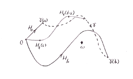
Figure 1: A symmetric $\Omega$-homotopy, with its initial path $H_{a}$, its final path $H_{b}$ and its endpointpath $\gamma={\Gamma}_{H}$.

The first two conditions imply that each path $H_{t}$ is a path of analytic continuation for any $\hat{\varphi}\in\hat{\mathscr{R}}_{\Omega}$, in view of Remark 2.2.

We shall use the notation $H_{t|s}$ for the truncated paths $(H_{t})_{|[0,s]}$, $s\in I$, $t\in J$ (analogously to what we did when commenting Lemma 3.1). Here is a technical statement we shall use:

Lemma 5.2.

For a symmetric $\Omega$-homotopy $H$ defined on $I\times J$, there exists $\delta>0$ such that, for any $\hat{\varphi}\in\hat{\mathscr{R}}_{\Omega}$ and $(s,t)\in I\times J$, the radius of convergence of the holomorphic germ $\operatorname{cont}_{H_{t|s}}\hat{\varphi}$ at $H_{t}(s)$ is at least $\delta$.

Proof.

Let $\rho$ be as in Remark 2.2. Consider

$$U\coloneqq\big{\{}\,(s,t)\in I\times J\mid H\big{(}[0,s]\times\{t\}\big{)}\subset\mathbb{D}_{\rho/2}\,\},\qquad K\coloneqq I\times J\setminus U.$$

Writing $K=\big{\{}\,(s,t)\in I\times J\mid\exists s^{\prime}\in[0,s]\;\text{s.t.}\;H(s^{\prime},t)\in\mathbb{C}\setminus\mathbb{D}_{\rho/2}\,\}$, we see that $K$ is a compact subset of $I\times J$ which is contained in $(0,1]\times J$. Thus $H(K)$ is a compact subset of $\mathbb{C}\setminus\Omega$, and $\delta\coloneqq\min\big{\{}\operatorname{dist}\big{(}H(K),\Omega\big{)},\rho/2\big{\}}>0$. Now, for any $s$ and $t$,

1. either $(s,t)\in U$, then the truncated path $H_{t|s}$ lies in $\mathbb{D}_{\rho/2}$, hence $\operatorname{cont}_{H_{t|s}}\hat{\varphi}$ is a holomorphic germ at $H_{t}(s)$ with radius of convergence $\geq\delta$;

2. or $(s,t)\in K$, and then $\operatorname{dist}(H_{t}(s),\Omega)\geq\delta$, which yields the same conclusion for the germ $\operatorname{cont}_{H_{t|s}}\hat{\varphi}$.

∎

The third condition in Definition 5.1 means that each path $H_{t}$ is symmetric with respect to its midpoint $\frac{1}{2}H_{t}(1)$. Here is the motivation behind this requirement:

Lemma 5.3.

Let $\gamma\colon\thinspace[0,1]\to\mathbb{C}\setminus\Omega$ be a path such that $\gamma(0)\in\mathbb{D}_{\rho}$, with $\rho$ as in Remark 2.2. If there exists a symmetric $\Omega$-homotopy whose endpoint path coincides with $\gamma$ and whose initial path is contained in $\mathbb{D}_{\rho}$, then any convolution product $\hat{\varphi}*\hat{\psi}$ with $\hat{\varphi},\hat{\psi}\in\hat{\mathscr{R}}_{\Omega}$ can be analytically continued along $\gamma$.

Proof.

We assume that $H$ is defined on $I\times J$ and we set $\gamma\coloneqq{\Gamma}_{H}$. Let $\hat{\varphi},\hat{\psi}\in\hat{\mathscr{R}}_{\Omega}$ and, for $t\in J$, consider the formula

$$\hat{\chi}_{t}({\zeta})=\int_{H_{t}}\hat{\varphi}(\xi)\hat{\psi}({\zeta}-\xi)\,{\mathrm{d}}\xi+\int_{\gamma(t)}^{\zeta}\hat{\varphi}(\xi)\hat{\psi}({\zeta}-\xi)\,{\mathrm{d}}\xi$$ (3)

(recall that $\gamma(t)=H_{t}(1)$). We shall check that $\hat{\chi}_{t}$ is a well-defined holomorphic germ at $\gamma(t)$ and that it provides the analytic continuation of $\hat{\varphi}*\hat{\psi}$ along $\gamma$.

a) The idea is that when $\xi$ moves along $H_{t}$, $\xi=H_{t}(s)$ with $s\in I$, we can use for “$\hat{\varphi}(\xi)$” the analytic continuation of $\hat{\varphi}$ along the truncated path $H_{t|s}$; correspondingly, if ${\zeta}$ is close to $\gamma(t)$, then ${\zeta}-\xi$ is close to $\gamma(t)-\xi=H_{t}(1)-H_{t}(s)=H_{t}(1-s)$, thus for “$\hat{\psi}({\zeta}-\xi)$” we can use the analytic continuation of $\hat{\psi}$ along $H_{t|1-s}$. In other words, setting ${\zeta}=\gamma(t)+{\sigma}$, we wish to interpret (3) as

$$\hat{\chi}_{t}(\gamma(t)+{\sigma})\coloneqq\int_{0}^{1}(\operatorname{cont}_{H_{t|s}}\hat{\varphi})(H_{t}(s))(\operatorname{cont}_{H_{t|1-s}}\hat{\psi})(H_{t}(1-s)+{\sigma})H_{t}^{\prime}(s)\,{\mathrm{d}}s\\ +\int_{0}^{1}(\operatorname{cont}_{H_{t}}\hat{\varphi})(\gamma(t)+u{\sigma})\hat{\psi}((1-u){\sigma}){\sigma}\,{\mathrm{d}}u$$ (4)

(in the last integral, we have performed the change variable $\xi=\gamma(t)+u{\sigma}$; it is the germ of $\hat{\psi}$ at the origin that we use there).

Lemma 5.2 provides $\delta>0$ such that, by regular dependence of the integrals upon the parameter ${\sigma}$, the right-hand side of (4) is holomorphic for $|{\sigma}|<\delta$. We thus have a family of analytic elements $(\hat{\chi}_{t},D_{t})$, $t\in J$, with $D_{t}\coloneqq D\big{(}\gamma(t),\delta\big{)}$.

b) For $t$ small enough, the path $H_{t}$ is contained in $\mathbb{D}_{\rho}$ which is open and simply connected; then, for $|{\zeta}|$ small enough, the line segment $[0,{\zeta}]$ and the concatenation of $H_{t}$ and $[\gamma(t),{\zeta}]$ are homotopic in $\mathbb{D}_{\rho}$, hence the Cauchy theorem implies $\hat{\chi}_{t}({\zeta})=\hat{\varphi}*\hat{\psi}({\zeta})$.

c) By uniform continuity, there exists ${\varepsilon}>0$ such that, for any $t_{0},t\in J$,

$$|t-t_{0}|\leq{\varepsilon}\quad\Longrightarrow\quad|H_{t}(s)-H_{t_{0}}(s)|<\delta/2\quad\text{for all $s\in I$}.$$ (5)

To complete the proof, we check that, for any $t_{0},t$ in $J$ such that $t_{0}\leq t\leq t_{0}+{\varepsilon}$, we have $\hat{\chi}_{t_{0}}\equiv\hat{\chi}_{t}$ in $D\big{(}\gamma(t_{0}),\delta/2)$ (which is contained in $D_{t_{0}}\cap D_{t}$).

Let $t_{0},t\in J$ be such that $t_{0}\leq t\leq t_{0}+{\varepsilon}$ and let ${\zeta}\in D\big{(}\gamma(t_{0}),\delta/2)$. By Lemma 5.2 and (5), we have for every $s\in I$

$$\operatorname{cont}_{H_{t|s}}\hat{\varphi}\big{(}H_{t}(s)\big{)}=\operatorname{cont}_{H_{t_{0}|s}}\hat{\varphi}\big{(}H_{t}(s)\big{)},$$

$$\operatorname{cont}_{H_{t|1-s}}\hat{\psi}\big{(}{\zeta}-H_{t}(s)\big{)}=\operatorname{cont}_{H_{t_{0}|1-s}}\hat{\psi}\big{(}{\zeta}-H_{t}(s)\big{)}$$

(for the latter identity, write ${\zeta}-H_{t}(s)=H_{t}(1-s)+{\zeta}-\gamma(t)=H_{t_{0}}(1-s)+{\zeta}-\gamma(t_{0})+H_{t_{0}}(s)-H_{t}(s)$, thus this point belongs to $D\big{(}H_{t}(1-s),\delta)\cap D\big{(}H_{t_{0}}(1-s),\delta)$). Moreover, $[\gamma(t),{\zeta}]\subset D\big{(}\gamma(t_{0}),\delta/2)$ by convexity, hence $\operatorname{cont}_{H_{t}}\hat{\varphi}\equiv\operatorname{cont}_{H_{t_{0}}}\hat{\varphi}$ on this line segment, and we can write

$$\hat{\chi}_{t}({\zeta})=\int_{0}^{1}(\operatorname{cont}_{H_{t_{0}|s}}\hat{\varphi})(H_{t}(s))(\operatorname{cont}_{H_{t_{0}|1-s}}\hat{\psi})({\zeta}-H_{t}(s))H_{t}^{\prime}(s)\,{\mathrm{d}}s\\ +\int_{\gamma(t)}^{\zeta}(\operatorname{cont}_{H_{t_{0}}}\hat{\varphi})(\xi)\hat{\psi}({\zeta}-\xi)\,{\mathrm{d}}\xi.$$

We then get $\hat{\chi}_{t_{0}}({\zeta})=\hat{\chi}_{t}({\zeta})$ from the Cauchy theorem by means of the homotopy induced by $H$ between the concatenation of $H_{t_{0}}$ and $[\gamma(t_{0}),{\zeta}]$ and the concatenation of $H_{t}$ and $[\gamma(t),{\zeta}]$. ∎

Remark 5.4.

Definition 5.1 is not really new: when the initial path $H_{a}$ is a line segment contained in $\mathbb{D}_{\rho}$, the final path $H_{b}$ is what Écalle calls a “symmetrically contractile path” in [Eca81]. The proof of Lemma 5.3 shows that the analytic continuation of $\hat{\varphi}*\hat{\psi}$ until the endpoint $H_{b}(1)={\Gamma}_{H}(b)$ can be computed by the usual integral taken over $H_{b}$ (however, it usually cannot be computed as the same integral over the endpoint path ${\Gamma}_{H}$, even when the latter integral is well-defined).

6 Proof of the main result: Geometric part

6.1 The key lemma

In view of Lemma 5.3, the proof of Theorem 4.1 will be complete if we prove the following purely geometric result:

Lemma 6.1.

For any path $\gamma\colon\thinspace I=[0,1]\to\mathbb{C}\setminus\Omega$ such that $\gamma(0)\in\mathbb{D}^{*}_{\rho}$ and the left and right derivatives $\gamma^{\prime}_{\pm}$ do not vanish on $I$, there exists a symmetric $\Omega$-homotopy $H$ on $I\times I$ whose endpoint path is $\gamma$ and whose initial path is a line segment, i.e. ${\Gamma}_{H}=\gamma$ and $H_{0}(s)\equiv s\gamma(0)$.

The proof is strikingly simple when $\gamma$ does not pass through $0$, which is automatic if we assume $0\in\Omega$. The general case requires an extra work which is technical and involves a quantitative version of the simpler case. With a view to helping the reader to grasp the mechanism of the proof, we thus begin with the case when $0\in\Omega$.

6.2 Proof of the key lemma when $0\in\Omega$

Assume that $\gamma$ is given as in the hypothesis of Lemma 6.1. We are looking for a symmetric $\Omega$-homotopy whose initial path is imposed: it must be

$$s\in I\mapsto H_{0}(s)\coloneqq s\gamma(0),$$

which satisfies the three requirements of Definition 5.1 at $t=0$:

1. $H_{0}(0)=0$,

2. $H_{0}\big{(}(0,1]\big{)}\subset\mathbb{C}\setminus\Omega$,

3. $H_{0}(1)-H_{0}(s)=H_{0}(1-s)$ for every $s\in I$.

The idea is to define a family of maps $(\Psi_{t})_{t\in[0,1]}$ so that

$$H_{t}(s)\coloneqq\Psi_{t}\big{(}H_{0}(s)\big{)},\qquad s\in I,$$ (6)

yield the desired homotopy. For that, it is sufficient that $(t,{\zeta})\in[0,1]\times\mathbb{C}\mapsto\Psi_{t}({\zeta})$ be continuously differentiable (for the structure of real two-dimensional vector space of $\mathbb{C}$), $\Psi_{0}=\mathop{\hbox{{\rm Id}}}\nolimits$ and, for each $t\in[0,1]$,

1. $\Psi_{t}(0)=0$,

2. $\Psi_{t}(\mathbb{C}\setminus\Omega)\subset\mathbb{C}\setminus\Omega$,

3. $\Psi_{t}\big{(}\gamma(0)-{\zeta}\big{)}=\Psi_{t}\big{(}\gamma(0)\big{)}-\Psi_{t}({\zeta})$ for all ${\zeta}\in\mathbb{C}$,

4. $\Psi_{t}\big{(}\gamma(0)\big{)}=\gamma(t)$.

In fact, the properties (i’)–(iv’) ensure that any initial path $H_{0}$ satisfying (i)–(iii) and ending at $\gamma(0)$ produces through (6) a symmetric $\Omega$-homotopy whose endpoint path is $\gamma$. Consequently, we may assume without loss of generality that $\gamma$ is $C^{1}$ on $[0,1]$ (then, if $\gamma$ is only piecewise $C^{1}$, we just need to concatenate the symmetric $\Omega$-homotopies associated with the various pieces).

The maps $\Psi_{t}$ will be generated by the flow of a non-autonomous vector field $X({\zeta},t)$ associated with $\gamma$ that we now define. We view $(\mathbb{C},|\,\cdot\,|)$ as a real $2$-dimensional Banach space and pick a $C^{1}$ function $\eta\colon\thinspace\mathbb{C}\to[0,1]$ such that

$$\{\,{\zeta}\in\mathbb{C}\mid\eta({\zeta})=0\,\}=\Omega.$$

Observe that $D({\zeta},t)\coloneqq\eta({\zeta})+\eta\big{(}\gamma(t)-{\zeta}\big{)}$ defines a $C^{1}$ function of $({\zeta},t)$ which satisfies

$$D({\zeta},t)>0\quad\text{for all ${\zeta}\in\mathbb{C}$ and $t\in[0,1]$}$$

because $\Omega$ is stable under addition; indeed, $D({\zeta},t)=0$ would imply ${\zeta}\in\Omega$ and $\gamma(t)-{\zeta}\in\Omega$, hence $\gamma(t)\in\Omega$, which would contradict our assumptions. Therefore, the formula

$$X({\zeta},t)\coloneqq\frac{\eta({\zeta})}{\eta({\zeta})+\eta\big{(}\gamma(t)-{\zeta}\big{)}}\gamma^{\prime}(t)$$ (7)

defines a non-autonomous vector field, which is continuous in $({\zeta},t)$ on $\mathbb{C}\times[0,1]$, $C^{1}$ in ${\zeta}$ and has its partial derivatives continuous in $({\zeta},t)$. The Cauchy-Lipschitz theorem on the existence and uniqueness of solutions to differential equations applies to $\frac{{\mathrm{d}}{\zeta}}{{\mathrm{d}}t}=X({\zeta},t)$: for every ${\zeta}\in\mathbb{C}$ and $t_{0}\in[0,1]$ there is a unique solution $t\mapsto\Phi^{t_{0},t}({\zeta})$ such that $\Phi^{t_{0},t_{0}}({\zeta})={\zeta}$. The fact that the vector field $X$ is bounded implies that $\Phi^{t_{0},t}({\zeta})$ is defined for all $t\in[0,1]$ and the classical theory guarantees that $(t_{0},t,{\zeta})\mapsto\Phi^{t_{0},t}({\zeta})$ is $C^{1}$ on $[0,1]\times[0,1]\times\mathbb{C}$.

Let us set $\Psi_{t}\coloneqq\Phi^{0,t}$ for $t\in[0,1]$ and check that this family of maps satisfies (i’)–(iv’). We have

$$X(\omega,t)=0\quad\text{for all $\omega\in\Omega$,}$$ (8)

$$X\big{(}\gamma(t)-{\zeta},t\big{)}=\gamma^{\prime}(t)-X({\zeta},t)\quad\text{for all ${\zeta}\in\mathbb{C}$}$$ (9)

for all $t\in[0,1]$ (by the very definition of $X$). Therefore

• (i’) and (ii’) follow from (8) which yields $\Phi^{t_{0},t}(\omega)=\omega$ for every $t_{0}$ and $t$, whence $\Psi_{t}(0)=0$ since $0\in\Omega$, and from the non-autonomous flow property $\Phi^{t,0}\circ\Phi^{0,t}=\mathop{\hbox{{\rm Id}}}\nolimits$ (hence $\Psi_{t}({\zeta})=\omega$ implies ${\zeta}=\Phi^{t,0}(\omega)=\omega$);

• (iv’) follows from the fact that $X\big{(}\gamma(t),t\big{)}=\gamma^{\prime}(t)$, by (8) and (9) with ${\zeta}=0$, using again that $0\in\Omega$, hence $t\mapsto\gamma(t)$ is a solution of $X$;

• (iii’) follows from (9): for any solution $t\mapsto{\zeta}(t)$, the curve $t\mapsto\xi(t)\coloneqq\gamma(t)-{\zeta}(t)$ satisfies $\xi(0)=\gamma(0)-{\zeta}(0)$ and $\xi^{\prime}(t)=\gamma^{\prime}(t)-X\big{(}{\zeta}(t),t\big{)}=X\big{(}\xi(t),t\big{)}$, hence it is a solution: $\xi(t)=\Psi_{t}\big{(}\gamma(0)-{\zeta}(0)\big{)}$.

As explained above, formula (6) thus produces the desired symmetric $\Omega$-homotopy.

Remark 6.2.

Our proof of Lemma 6.1, which essentially relies on the use of the flow of the non-autonomous vector field (7), arose as an attempt to understand a related but more complicated construction which can be found in an appendix of the book [CNP93] (however the vector field there was autonomous and we must confess that we were not able to follow completely the arguments of [CNP93]).

6.3 Proof of the key lemma when $0\notin\Omega$

From now on, we suppose $0\notin\Omega$ and we use the notation

$$\Omega_{\varepsilon}\coloneqq\{\,{\zeta}\in\mathbb{C}\mid\operatorname{dist}({\zeta},\Omega)<{\varepsilon}\,\}$$

for any ${\varepsilon}>0$, hence $\overline{\Omega}_{{\varepsilon}}=\{\,{\zeta}\in\mathbb{C}\mid\operatorname{dist}({\zeta},\Omega)\leq{\varepsilon}\,\}$. We shall require the following technical

Lemma 6.3.

For any ${\varepsilon}>0$ there exists a $C^{1}$ function $\eta\colon\thinspace\mathbb{C}\to[0,1]$ such that

$$\{\,{\zeta}\in\mathbb{C}\mid\eta({\zeta})=0\,\}=\{0\}\cup\overline{\Omega}_{{\varepsilon}}.$$

Proof.

Pick a $C^{1}$ function $\chi\colon\thinspace\mathbb{R}\to[0,1]$ such that $\{\,x\in\mathbb{R}\mid\chi(x)=0\,\}=[-{\varepsilon}^{2},{\varepsilon}^{2}]$ and $\chi(x)=1$ for $|x|\geq(1+{\varepsilon})^{2}$, and a bijection $\omega\colon\thinspace\mathbb{N}^{*}\to\Omega$. For each $k\in\mathbb{N}^{*}$, $\eta_{k}({\zeta})\coloneqq\chi\big{(}|{\zeta}-\omega(k)|^{2}\big{)}$ defines a $C^{1}$ function on $\mathbb{C}$ such that $\eta_{k}^{-1}(0)=\overline{D(\omega(k),{\varepsilon})}$ and $\eta_{k}\equiv 1$ on $\mathbb{C}\setminus D(\omega(k),1+{\varepsilon})$. Consider the infinite product

$$\eta_{*}({\zeta})\coloneqq\prod_{k\in\mathbb{N}^{*}}\eta_{k}({\zeta}).$$ (10)

For any bounded open subset $U$ of $\mathbb{C}$, the set $\mathcal{F}_{U}\coloneqq\{\,k\in\mathbb{N}^{*}\mid U\cap D(\omega(k),1+{\varepsilon})\neq\emptyset\,\}$ is finite (because $\Omega$ is discrete), thus almost all the factors in (10) are equal to $1$ when ${\zeta}\in U$: $(\eta_{*})_{|U}=\prod_{k\in\mathcal{F}_{U}}(\eta_{k})_{|U}$, hence $\eta_{*}$ is $C^{1}$, takes its values in $[0,1]$ and

$$\eta_{*}^{-1}(0)\cap U=\bigcup_{k\in\mathcal{F}_{U}}\overline{D(\omega(k),{\varepsilon})}\cap U,$$

whence it follows that $\eta_{*}^{-1}(0)=\overline{\Omega}_{{\varepsilon}}$.

If $0\in\overline{\Omega}_{\varepsilon}$, then one can take $\eta=\eta_{*}$. If not, then one can take the product $\eta=\eta_{0}\eta_{*}$ with $\eta_{0}({\zeta})\coloneqq\chi_{0}(|{\zeta}|^{2})$, where $\chi_{0}$ is any $C^{1}$ function on $\mathbb{R}$ which takes its values in $[0,1]$ and such that $\chi_{0}^{-1}(0)=\{0\}$. ∎

We now repeat the work of the previous section replacing $\Omega$ with $\{0\}\cup\Omega$, adding quantitative information (we still assume that we are given a path which does not pass through $0$ but we want to control the way the corresponding symmetric $\Omega$-homotopy approaches the points of $\Omega$) and authorizing a more general initial path than a rectilinear one.

Lemma 6.4.

Let $\delta,\delta^{\prime}>0$ with $\delta^{\prime}<\delta/2$. Suppose that $J=[a,b]$ is a compact interval of $\mathbb{R}$ and $\gamma\colon\thinspace J\to\mathbb{C}$ is a path such that

$$0\notin\gamma(J)\quad\text{and}\quad\gamma(J)\subset\mathbb{C}\setminus\Omega_{\delta}.$$

Suppose that $h\colon\thinspace I\to\mathbb{C}$ is a $C^{1}$ path such that

1. $h(0)=0$,

2. $h(I)\subset\mathbb{C}\setminus\Omega_{\delta^{\prime}}$,

3. $h(1-s)=h(1)-h(s)$ for all $s\in I$,

4. $h(1)=\gamma(a)$.

Then there exists a symmetric $\Omega$-homotopy $H$ defined on $I\times J$, whose initial path is $h$, whose endpoint path is $\gamma$, which satisfies $H(I\times J)\subset\mathbb{C}\setminus{\Omega_{\delta^{\prime}}}$ and whose final path is $C^{1}$.

Proof.

We may assume without loss of generality that $\gamma$ is $C^{1}$ on $J$ (if $\gamma$ is only piecewise $C^{1}$, we just need to concatenate the symmetric $\Omega$-homotopies associated with the various pieces). We shall define a family of maps $(\Psi_{t})_{t\in J}$ so that

$$H_{t}(s)\coloneqq\Psi_{t}\big{(}h(s)\big{)},\qquad s\in I,$$ (11)

yield the desired homotopy. For that, it is sufficient that $(t,{\zeta})\in J\times\mathbb{C}\mapsto\Psi_{t}({\zeta})$ be continuously differentiable, $\Psi_{0}=\mathop{\hbox{{\rm Id}}}\nolimits$ and, for each $t\in J$,

1. $\Psi_{t}(0)=0$,

2. $\Psi_{t}(\mathbb{C}\setminus\Omega_{\delta^{\prime}})\subset\mathbb{C}\setminus\Omega_{\delta^{\prime}}$,

3. $\Psi_{t}\big{(}\gamma(a)-{\zeta}\big{)}=\Psi_{t}\big{(}\gamma(a)\big{)}-\Psi_{t}({\zeta})$ for all ${\zeta}\in\mathbb{C}$,

4. $\Psi_{t}\big{(}\gamma(a)\big{)}=\gamma(t)$.

As in Section 6.2, our maps $\Psi_{t}$ will be generated by a non-autonomous vector field.

Lemma 6.3 allows us to choose a $C^{1}$ function $\eta\colon\thinspace\mathbb{C}\to[0,1]$ such that

$$\{\,{\zeta}\in\mathbb{C}\mid\eta({\zeta})=0\,\}=\{0\}\cup\overline{\Omega}_{\delta^{\prime}}.$$

We observe that $D({\zeta},t)\coloneqq\eta({\zeta})+\eta\big{(}\gamma(t)-{\zeta}\big{)}$ defines a $C^{1}$ function of $({\zeta},t)$ which satisfies

$$D({\zeta},t)>0\quad\text{for all ${\zeta}\in\mathbb{C}$ and $t\in[0,1]$}$$

because $\Omega$ is stable under addition; indeed, $D({\zeta},t)=0$ would imply that both ${\zeta}$ and $\gamma(t)-{\zeta}$ lie in $\{0\}\cup\overline{\Omega}_{\delta^{\prime}}$, hence $\gamma(t)\in\{0\}\cup\overline{\Omega}_{2\delta^{\prime}}$, which would contradict our assumption $\gamma(J)\subset\mathbb{C}\setminus\big{(}\{0\}\cup\Omega_{\delta}\big{)}$. Therefore the formula

$$X({\zeta},t)\coloneqq\frac{\eta({\zeta})}{\eta({\zeta})+\eta\big{(}\gamma(t)-{\zeta}\big{)}}\gamma^{\prime}(t),\qquad({\zeta},t)\in\mathbb{C}\times J,$$

defines a non-autonomous vector field whose flow $(\Phi^{t_{0},t})_{t_{0},t\in J}$ allows one to conclude the proof exactly as in Section 6.2, setting $\Psi_{t}\coloneqq\Phi^{a,t}$ and replacing (8) with

$$X(\omega,t)=0\quad\text{for all $\omega\in\{0\}\cup\Omega_{\delta^{\prime}}$.}$$

∎

We now consider the case of a path $\gamma$ which entirely lies close to $0$.

Lemma 6.5.

Let ${\varepsilon},\delta^{\prime}>0$ with $0<{\varepsilon}<\delta^{\prime}$. Suppose that $K=[a,b]$ is a compact interval of $\mathbb{R}$ and $\gamma\colon\thinspace K\to\mathbb{C}$ is a path such that

$$\gamma(K)\subset\overline{\mathbb{D}}_{{\varepsilon}/2}.$$

Suppose that $h\colon\thinspace I\to\mathbb{C}$ is a $C^{1}$ path such that

1. $h(0)=0$,

2. $h(I)\subset\mathbb{C}\setminus\Omega_{\delta^{\prime}}$,

3. $h(1-s)=h(1)-h(s)$ for all $s\in I$,

4. $h(1)=\gamma(a)$.

Then there exists a symmetric $\Omega$-homotopy $H$ defined on $I\times K$, whose initial path is $h$, whose endpoint path is $\gamma$, which satisfies

$$H(I\times K)\subset\mathbb{C}\setminus{\Omega_{\delta^{\prime\prime}}}\quad\text{ with $\delta^{\prime\prime}\coloneqq\delta^{\prime}-{\varepsilon}$ }$$

and whose final path is $C^{1}$.

Proof.

Define $H(s,t)\coloneqq h(s)+s\big{(}\gamma(t)-\gamma(a)\big{)}$. This way $H(s,a)=h(s)$, $H(1,t)=\gamma(t)$ and $H$ is a symmetric $\Omega$-homotopy as required: $H(0,t)=0$, $H(s,t)+H(1-s,t)=h(s)+h(1-s)+\gamma(t)-\gamma(a)=\gamma(t)$, $\operatorname{dist}\big{(}H(s,t),\Omega\big{)}\geq\operatorname{dist}\big{(}h(s),\Omega)-|\gamma(t)-\gamma(a)|\geq\delta^{\prime}-{\varepsilon}$. ∎

Proof of the key lemma when $0\notin\Omega$. Let $\gamma$ be as in the hypothesis of Lemma 6.1. Without loss of generality, we can assume $\gamma(1)\neq 0$ (if not, view $\gamma$ as the restriction of a path $\tilde{\gamma}\colon\thinspace[0,2]\to\mathbb{C}\setminus\Omega$ such that $\gamma(2)\neq 0$, with which is associated a symmetric $\Omega$-homotopy $\tilde{H}$ defined on $I\times[0,2]$, and restrict $\tilde{H}$ to $I\times[0,1]$). Let $\delta\coloneqq\operatorname{dist}\big{(}\Omega,\gamma([0,1])\big{)}$.

The set $Z\coloneqq\{\,t\in[0,1]\mid\gamma(t)=0\,\}$ is closed; it is also discrete because of the non-vanishing of the derivatives of $\gamma$, thus it has a finite cardinality $N\in\mathbb{N}$. If $N=0$, then we can apply Lemma 6.4 with $J=[0,1]$ and $h(s)\equiv s\gamma(0)$ and the proof is complete.

From now on we suppose $N\geq 1$. Let us write

$$Z=\{t_{1},\ldots,t_{N}\}\quad\text{with $0<t_{1}<\cdots<t_{N}<1$.}$$

We define

$$\delta_{0}\coloneqq\frac{1}{2}\min\Big{\{}\frac{\delta}{2},\rho-|\gamma(0)|\Big{\}}\quad\text{and}\quad{\varepsilon}\coloneqq\min\Big{\{}|\gamma(0)|,|\gamma(1)|,\frac{\delta_{0}}{N+1}\Big{\}}.$$

The continuity of $\gamma$ allows us to find pairwise disjoint closed intervals of positive lengths $K_{1},\ldots,K_{N}$ such that

$$t_{j}\in\mathring{K}_{j}\quad\text{and}\quad\gamma(K_{j})\subset\overline{\mathbb{D}}_{{\varepsilon}/2},\qquad j=1,\ldots,N.$$

By considering the connected components of $[0,1]\setminus\bigcup K_{j}$ and taking their closures, we get adjacent closed subintervals of positive lengths of $[0,1]$,

$$J_{0},K_{1},J_{1},K_{2},\ldots,J_{N-1},K_{N},J_{N}$$

with $J_{j}=[a_{j},b_{j}]$, $K_{j}=[b_{j-1},a_{j}]$, $a_{0}=0$, $b_{N}=1$. Observe that

$$0\notin\gamma(J_{j})\quad\text{and}\quad\gamma(J_{j})\subset\mathbb{C}\setminus\Omega_{\delta},\qquad j=0,\ldots,N.$$

• We apply Lemma 6.4 with $J=J_{0}=[0,b_{0}]$, $h(s)\equiv s\gamma(0)$ and $\delta^{\prime}=\delta_{0}$ (which is allowed by the choice of $\delta_{0}$): we get a symmetric $\Omega$-homotopy $H$ defined on $I\times J_{0}$ whose initial path is the line segment $[0,\gamma(0)]$, whose endpoint path is $\gamma_{|J_{0}}$ and whose final path $H_{b_{0}}$ is $C^{1}$ and lies in $\mathbb{C}\setminus\Omega_{\delta_{0}}$.

• We apply Lemma 6.5 with $K=K_{1}$, $\delta^{\prime}=\delta_{0}$ and $h=H_{b_{0}}$: we get an extension of our symmetric $\Omega$-homotopy $H$ to $I\times K_{1}$, in which the enpoint path is extended by $\gamma_{|K_{1}}$ and the final path is now $H_{a_{1}}$, a $C^{1}$ path contained in $\mathbb{C}\setminus\Omega_{\delta_{1}}$ with $\delta_{1}\coloneqq\delta_{0}-{\varepsilon}$.

• And so on: we apply alternatively Lemma 6.5 on $K_{j}$ and Lemma 6.4 on $J_{j}$: we get an extension of the symmetric $\Omega$-homotopy $H$ to $I\times K_{j}$ or $I\times J_{j}$ such that both $H_{a_{j}}(I)$ and $H_{b_{j}}(I)$ are contained in $\mathbb{C}\setminus\Omega_{\delta_{j}}$ with $\delta_{j}\coloneqq\delta_{0}-j{\varepsilon}$.

When we reach $j=N$, the proof of Lemma 6.1 is complete.

Acknowledgements. The author wishes to thank the anonymous referee for helping to improve this article. The research leading to these results has received funding from the European Comunity’s Seventh Framework Program (FP7/2007–2013) under Grant Agreement n. 236346.

David Sauzin
CNRS UMI 3483 - Laboratorio Fibonacci
Collegio Puteano, Scuola Normale Superiore di Pisa
Piazza dei Cavalieri 3, 56126 Pisa, Italy
email: david.sauzin@sns.it

References

- [1]
- [CNP93] B. Candelpergher, J.-C. Nosmas and F. Pham. Approche de la résurgence. Actualités Math., Hermann, Paris, 1993.
- [DS12] A. Dudko and D. Sauzin. Écalle-Voronin invariants via resurgence and alien calculus. In preparation.
- [Eca81] J. Écalle. Les fonctions résurgentes. Publ. Math. d’Orsay, Vol. 1: 81-05, Vol. 2: 81-06, Vol. 3: 85-05, 1981, 1985.
- [Eca84] J. Écalle. Cinq applications des fonctions résurgentes. Publ. Math. d’Orsay 84-62, 1984.
- [Eca92] J. Écalle. Introduction aux fonctions analysables et preuve constructive de la conjecture de Dulac. Actualités Math., Hermann, Paris, 1992.
- [Eca93] J. Écalle. Six lectures on Transseries, Analysable Functions and the Constructive Proof of Dulac’s conjecture. D.Schlomiuk (ed.), Bifurcations and Periodic Orbits of Vector Field, pp. 75–184, Kluwer Ac. Publishers, 1993.
- [Mal85] B. Malgrange. Introduction aux travaux de J. Écalle. L’Enseign. Math. (2) 31, 3–4 (1985), 261–282.
- [Ou10] Y. Ou. On the stability by convolution product of a resurgent algebra. Ann. Fac. Sci. Toulouse (6) 19, 3–4 (2010), 687–705.
- [Sau06] D. Sauzin, Resurgent functions and splitting problems. RIMS Kokyuroku 1493 (2005), 48–117.
- [Sau10] D. Sauzin, Mould expansions for the saddle-node and resurgence monomials. In Renormalization and Galois theories. Selected papers of the CIRM workshop, Luminy, France, March 2006, p. 83–163, A. Connes, F. Fauvet, J.-P. Ramis (eds.), IRMA Lectures in Mathematics and Theoretical Physics 15, Zürich: European Mathematical Society, 2009.
- [Sau12] D. Sauzin, Introduction to -summability and the resurgence theory. In preparation.