Constraining $H_{0}$ from Lyman-$\alpha$ Forest and Baryon Acoustic Oscillations

Abstract

A new method is proposed to measure the Hubble constant $H_{0}$ through the mean transmitted flux observed from high redshift quasars. A semi-analytical model for the cosmological-independent volume density distribution function is adopted which allows one to obtain constraints over the cosmological parameters once a moderate knowlegde of the InterGalactic Medium (IGM) parameters is assumed. By assuming a flat $\Lambda$CDM cosmology, we show that such method alone cannot provide good constraints on the pair of free parameters ($h,\Omega_{m}$). However, it is possible possible to break the degeneracy on the mass density parameter by applying a joint analysis involving the baryon acoustic oscillations (BAOs). Our analysis based on two different samples of Lyman-$\alpha$ forest resctricts ($h,\Omega_{m}$) on the intervals $0.58\leq h\leq 0.91$ and $0.215\leq\Omega_{m}\leq 0.245$ ($1\sigma$). Although the constraints are weaker comparatively to other estimates, we point out that with a bigger sample and a better knowledge of the IGM this method may present competitive results to measure the Hubble constant independently of the cosmic distance ladder.

1 Introduction

Measurements of the Hubble constant $H_{0}$ are vital to the establishment of a cosmic concordance model in cosmology. Such constant plays a role in most of cosmic calculations, as the age of the Universe, its size and energy density, primordial nucleosynthesis, physical distances to objects and so on. Its importance must even increase in the next decade because new missions and observational projects are being designed to provide accurate measurements of the Hubble constant thereby also increasing the precision in the other cosmological parameters.

There are several ways to determine $H_{0}$ by using low and high redshift sources. The most commom methods are based on the period-luminosity relation seen in Cepheids, tip of the red giant branch and Supernovae observed in the local Universe (Freedman & Madore 2010). However, some alternative procedures like the Sunyaev–Zel’dovich effect combined with X-ray emission from clusters allow a measurement of $H_{0}$ from high-redshift objects have also been discussed (Cunha et al. 2007, Holanda et al. 2010). Although considering that some errors recently reported in the literature are small (e.g. Riess et al. 2009), discrepancies among different measurements as the value given by Sandage et al. (2006) show that independent estimates are needed in order to achieve a reliable value for $H_{0}$ not plagued by systematic errors from astrophysical environments, as well as from calibrations associated to the cosmic distance ladder. In this concern, the importance and cosmological interest on different estimates of $H_{0}$ independent of the distance ladder has also been discussed by many authors (see Jackson 2007 and Refs. therein for a recent review).

A possible alternative procedure to measure $H_{0}$ is to consider the Lyman-$\alpha$ (Ly$\alpha$ ) forest data that probes the low density intergalatic medium (IGM) over a unique range of redshifts and environments as seen in the spectra from high redshift quasars. The observed mean transmitted flux depends on the local optical depth, which in turn depends on the expansion rate of the Universe $H(z)$ and some properties characterizing the intervening medium along our line of sight to any quasar. In principle, with a moderate knowledge of the IGM properties, as the hydrogen photoionization rate and mean temperature, the values of some cosmological parameters including the Hubble constant can be constrained.

In the last decade, several studies based on Ly$\alpha$ forests as cosmological tools have been performed (Macdonald et al. 2000, Weinberg et al. 2003, Wyithe et al. 2008, Viel et al. 2009). Some works use the flux power spectrum of the Ly$\alpha$ forest to infer the cosmological parameters in two ways: inversion of the flux power spectrum to get the underlying dark matter power spectrum (Croft et al., 1998, 1999; Hui, 1999; Nusser & Haehnelt, 1999), or to use the power spectrum directly (McDonald et al., 2000, 2005; Mandelbaum et al., 2003).

On the other hand, a simpler approach is to adopt a semi-analytical model to describe the IGM as proposed by Miralda-Escudé et al. (2000), who derived a fitting formula for the volume density distribution function in agreement with simulations which provided similar results for different numerical methods and different cosmologies (Rauch et al., 1997). Therefore, a theoretical mean transmitted flux is obtained and compared to observational data in order to constrain the cosmological parameters.

In this letter, by assuming a flat $\Lambda$CDM cosmology, we apply the above described procedure for deriving new constraints on the Hubble constant $H_{0}$ and the matter density parameter $\Omega_{m}$. By considering two independent samples of Ly$\alpha$ forest as compiled by Bergeron et al. (2004) and Guimarães et al. (2007), respectively, two distinct statistical analyses are performed. Firstly, we consider only the Ly$\alpha$ forest data set whereas the second approach involves a joint analysis combining the Ly$\alpha$ forest data with the SDSS measurements of the baryon acoustic peak from the clustering of luminous red galaxies (Eisenstein, 2005). As we shall see, the degeneracy on the free parameters defining the ($h,\Omega_{m}$) plane is naturally broken when the Ly$\alpha$ data are combined with the standard ruler as given by the baryon acoustic oscilations thereby providing a new independent method to estimate the Hubble parameter.

2 The Ly$\alpha$ Forest Samples

As remarked earlier, in the present analysis we consider two different samples. The first one consists of 18 high-resolution high signal-to-noise ratio (S/N) spectra. The spectra were obtained with the Ultra-Violet and Visible Echelle Spectrograph (UVES) mounted on the ESO KUEYEN 8.2 m telescope at the Paranal observatory for the ESO-VLT Large Programme (LP) ’Cosmological evolution of the Inter Galactic Medium’ (PI Jacqueline Bergeron; Bergeron et al. 2004). The spectra were taken from the European Southern Observatory archive and are publicly available. This programme has been devised to gather a homogeneous sample of echelle spectra of 18 QSOs, with uniform spectral coverage, resolution and signal-to-noise ratio suitable for studying the IGM. The spectra have a signal-to-noise ratio of 40 to 80 per pixel and a spectral resolution $\lambda/\Delta\lambda\sim 45000$ in the Ly$\alpha$ forest region. Details of the procedure used for data reduction can be found in Chand et al. (2004) and Aracil et al. (2004).

The second sample consists of 45 quasars obtained by Guimarães et al. (2007), where the spectra were measured with the ESI (Sheinis et al., 2002) mounted on the Keck II 10m telescope. The spectral resolution is $R\sim 4300$ with a signal-to-noise ratio usually larger than 15 per 10 km s^-1 pixel. This sample has also been studied Prochaska and collaborators (2003a,b) in their discussions related to the existence of Damped Ly$\alpha$ systems. In the present analysis we have used the Ly$\alpha$ forest over the rest-wavelenght range 1070-1170 Å  to avoid contamination by the proximity effect close to the Ly$\alpha$ emission line and possible OVI associated absorbers. We also carefully avoided regions flagged because of damped/sub-damped Ly$\alpha$ absorption lines. We divided each spectrum in bins of length $100$ Å  in the observed frame, corresponding to about $\triangle z=0.08$, for the last bin we have used a lenght of $500$ Å  to keep the statistical homogeneity. The mean transmitted flux was calculated as the mean flux over all pixels in a bin. At each redshift, we then averaged the transmitted fluxes over all spectra covering this redshift.

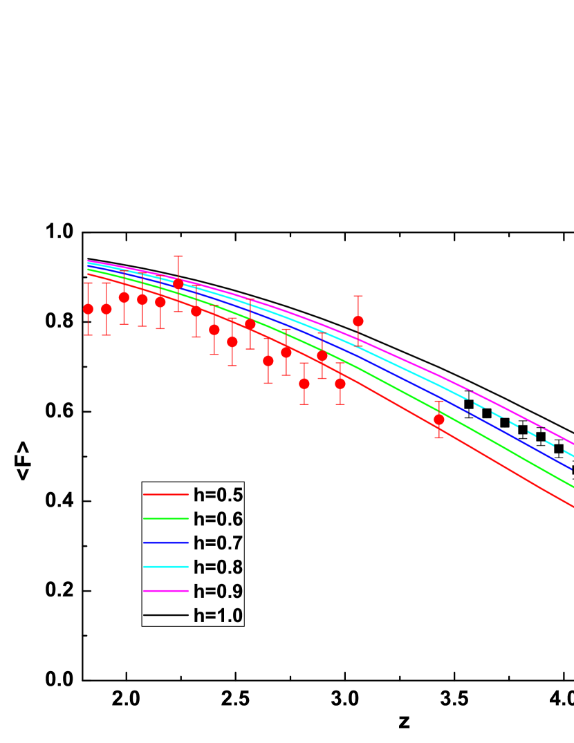
Figure 1: Mean transmitted flux as a function of redshift for $\Omega_{m}=0.23$, $\Gamma=0.8\times 10^{-12}$ s^-1, $T_{0}=2.5\times 10^{4}$ K and some selected values of the $h$ parameter. The data points correspond to the Ly$\alpha$ forest measurements obtained by this work (red circles) and Guimarães et al. (2007) (black squares).

In Fig 1, we display the mean transmitted flux for the two samples. Notice that all errors were estimated as the standard deviation of the mean values divided by the square root of the number of spectra. The corresponding scatter in the transmitted flux cannot be explained by photon noise or by uncertainties in the continuum thereby suggesting that errors are dominated by cosmic variance.

3 Basic Equations

The basic measurement obtained from the Ly$\alpha$ forest is the mean transmitted flux at redshift $z$ defined as

$$\langle F\rangle(z)\equiv\langle\exp{(-\tau(z))}\rangle,$$ (1)

where $\tau(z)$ is the local optical depth and angle brackets denote an average over the line of sight. Following standard lines (Hui & Gnedin, 1997), throughout this paper photoionization equilibrium and a power-law temperature-density relation, $T=T_{0}(1+\delta)^{\beta}$, for the low-density IGM will be assumed, where $\delta$ stands for the local overdensity and $T_{0}$ for the IGM temperature at mean density ($\delta=0$). The local optical depth is given by (Peebles, 1993; Padmanabhan, 2002; Faucher-Giguère et al., 2008a)

$$\tau(z)=A(z)(1+\delta)^{2-0.75\beta},$$ (2)

with

$$A(z)\equiv\frac{\pi e^{2}f_{Ly\alpha}}{m_{e}\nu_{Ly\alpha}}\left(\frac{\rho_{\rm crit}\Omega_{b}}{m_{p}}\right)^{2}\frac{X(X+0.5Y)}{H(z)}\frac{R_{0}T_{0}^{-0.75}}{\Gamma}(1+z)^{6}.$$ (3)

In the expression above, $f_{Ly\alpha}$ is the oscillator strength of the Ly$\alpha$  transition, $\nu_{Ly\alpha}$ is its frequency, $m_{e}$ and $m_{p}$ are the electron and proton masses respectively, $\Omega_{b}$ is the baryon density parameter, $H(z)$ is the Hubble parameter, $\rho_{\rm crit}$ is the critical density, $X$ and $Y$ are the mass fractions of hydrogen and helium respectively taken to be 0.75 and 0.25 (Burles et al., 2001), $R_{0}=4.2\times 10^{-13}~{}{\rm cm}^{3}~{}{\rm s}^{-1}/(10^{4}~{}{\rm K})^{-0.75}$ and $\Gamma$ is the hydrogen photoionization rate.

The mean transmitted flux is obtained by integrating the local optical depth through a volume density distribution function for the gas $\Delta\equiv 1+\delta$,

$$\langle F\rangle(z)=\int_{0}^{\infty}d\Delta P(\Delta;z)\exp{[-\tau(z)]}.$$ (4)

As is widely known, Miralda-Escudé et al. (2000) derived an approximate analytical functional form for the distribution function given by

$$P(\Delta;z)=A\exp{\left[-\frac{(\Delta^{-2/3}-C_{0})^{2}}{2(2\delta_{0}/3)^{2}}\right]}\Delta^{-b},$$ (5)

where the parameters $A$ and $C_{0}$ are derived by requiring the total volume and mass to be normalized to unity. Miralda-Escudé et al. (2000) extrapolated the distribution function and obtained $\delta_{0}=7.61/(1+z)$ with an accuracy better than 1% from fits to a numerical simulation at $z=$2, 3, and 4 from Miralda-Escudé et al. (1996). In order to apply this formalism to our data, the values of $b$ were derived from a cubic interpolation from the values in the simulation. Applications of this distribution function to constrain cosmological parameters is well justified since simulations with different numerical methods and different cosmologies provided very similar results (Rauch et al., 1997).

From now on a flat $\Lambda$CDM cosmology will be assumed. In this case, the Hubble parameter is given by

$$H(z)=H_{0}\left[\Omega_{m}(1+z)^{3}+(1-\Omega_{m})\right]^{1/2},$$ (6)

where we will adopt the convention $h=H_{0}/100$ km s^-1 Mpc^-1, which is the Hubble constant normalized in units of $100$ km s^-1 Mpc^-1.

The effects of $H_{0}$ in the mean transmitted flux are shown in Fig. 1 along with our observational data (red circles) and Guimarães et al. (2007) (black squares). We see that with our sample we obtain a scattered data set comparatively to the sample used by Guimarães et al. (2007), which is related to the sample size. It is also evident that our data cover most of values for the $h$ parameter, so we do not expect tight constraints from the Ly$\alpha$ data set alone.

4 Analyses and Results

Let us now perform a statistical analysis to find the constraints on the cosmological parameters. The full set of parameters are represented by $\mathbf{p}\equiv(h,\Omega_{m},\Gamma,T_{0},\Omega_{b}h^{2},\beta)$. We fix the value of $\Omega_{b}h^{2}=0.0218$ using the latest observations of deuterium (Pettini et al., 2008) from the Big Bang Nucleosynthesis (Simha & Steigman, 2008). An early reionization model is also considered which gives $\beta=0.62$ (Hui & Gnedin, 1997). The posterior probability of the parameters $P(\mathbf{p}|d)$ given the data $d$ is

$$P(\mathbf{p}|d)=\frac{P(d|\mathbf{p})P(\mathbf{p})}{P(d)},$$ (7)

where $P(d)$ is a normalization constant, $P(\mathbf{p})$ is the prior over the parameters and $P(d|\mathbf{p})\propto e^{-\chi^{2}/2}$ is the likelihood with the usual definition, for the Ly$\alpha$ forest data, of

$$\chi^{2}_{Ly\alpha}=\sum_{i}{(\langle F_{th}\rangle(z_{i};\mathbf{p})-\langle F\rangle(z_{i}))^{2}\over\sigma_{\langle F\rangle(z_{i})}^{2}},$$ (8)

where $\langle F_{th}\rangle(z_{i};\mathbf{p})$ is the theoretical mean transmitted flux, $\langle F\rangle(z_{i})$ is the observational mean transmitted flux and $\sigma_{\langle F\rangle(z_{i})}$ is its respective uncertainty. We treat the combination $\Gamma T_{0}^{0.75}$ as a nuisance parameter with a flat prior. The ranges chosen are $T_{0}=[2,2.5]\times 10^{4}$ K from estimates of Zaldarriaga et al. (2001) and $\Gamma=[0.8,1]\times 10^{-12}$ s^-1 which cover some measurements reported in the literature (Rauch et al., 1997; McDonald & Miralda-Escudé, 2001; Meiksin & White, 2004; Tytler et al., 2004; Bolton et al., 2005; Kirkman et al., 2005), although in disagreement with the values obtained by Faucher-Giguère et al. (2008a, b), who used a redshift-dependent relation for $T_{0}$ not favoured by our data.

In what follows, we first consider the Ly$\alpha$ forest data separately, and, further, we present a joint analysis including the BAO signature extracted from the SDSS catalog (Eisenstein et al. 2005).

4.1 Limits from Ly$\alpha$ Forest data set

In Fig. 2 we display the results of the statistical analysis performed with the Ly$\alpha$ forest data. We see that the data do not provide good constraints to both parameters. Several sanity checks were performed in order to determine the values fixed in the statistical analysis. In particular, we have seen that different values for $\beta$, different intervals for $\Gamma T_{0}^{-0.75}$ in the marginalization, or even a redshift-dependence for $T_{0}$, have resulted in poorer fits compared to what is shown in figure 2. In addition, even considering that cosmological constraints are affected by the IGM physical parameters the opposite vision is also true, that is, different cosmologies may also provide results not compatible for the IGM parameters. In this context, it is recommended to fit cosmological and IGM parameters together in order to obtain more trustful results.

Despite the considerations discussed above, we see from Fig. 2 that the slope in the $(h,\Omega_{m})$ plane suggests that a joint analysis with an independent test constraining only $\Omega_{m}$ could provide interesting limits to the Hubble parameter. Thus, a joint analysis with the BAO data is presented in the next subsection.

4.2 Ly$\alpha$ Forest and BAO: A Joint Analysis

In order to achieve better constraints on the cosmic parameters we apply a joint analysis involving Ly$\alpha$ forest data and baryon acoustic oscillations data obtained from 46748 luminous red galaxies selected from the SDSS Main Sample. The BAO scale can be represented by the parameter (Eisenstein, 2005)

$${\cal{A}}\equiv{\Omega_{\rm{m}}^{1/2}\over{{\cal{H}}(z_{\rm{*}})}^{1/3}}\left[\frac{1}{z_{\rm{*}}}\Gamma(z_{*})\right]^{2/3}=0.469\pm 0.017,$$ (9)

where $z_{\rm{*}}=0.35$ is the redshift at which the acoustic scale has been measured, ${\cal{H}}(z)$ is $H(z)/H_{0}$ and $\Gamma(z_{*})$ is the dimensionless comoving distance to $z_{*}$.

From equation (9) it is seen that the BAO scale is independent of $h$ thereby yielding constraints only for the matter density parameter. The statistical analysis is performed with $\chi^{2}=\chi^{2}_{Ly\alpha}+\chi^{2}_{BAO}$, where

$$\chi^{2}_{BAO}=\left(\frac{{\cal{A}}-0.469}{0.017}\right)^{2}.$$ (10)

In Fig. 3, we show the limits on the pair of parameters $(h,\Omega_{m})$ obtained from our joint analysis involving Ly$\alpha$ forest data and BAO. Within 68.3% confidence level, we have obtained $0.215\leq\Omega_{m}\leq 0.245$ and $0.58\leq h\leq 0.91$. The value for $\Omega_{m}$ is lower than what was found by other observations (e.g. Amanullah et al., 2010), but it is likely that the difference is due to systematic errors not taken into account in our analysis.

In Tab. 1, we show some recent measurements of $H_{0}$ using different techniques and data. Although existing a tension among different estimates (e.g. Sandage et al., 2006; Paraficz & Hjorth, 2010), our approach do not provide stringent limits which would allow a decision about the correct value of $H_{0}$. The interesting aspect is that the method discussed here provides an independent estimate which is in agreement with the values obtained adopting different approaches (see Table 1).

5 Conclusions

In this work we have used a cosmological-independent semi-analytical model to describe the IGM and data from Ly$\alpha$ forest and baryon acoustic oscillations to constrain cosmological parameters. Limits on the Hubble constant $H_{0}$ and the matter density parameter $\Omega_{m}$ were derived by assuming a flat $\Lambda$CDM cosmology.

By applying a statistical analysis using only the Ly$\alpha$ forest data we did not obtain good constraints to both parameters. However, when we applied a joint analysis involving the Ly$\alpha$ forest data and BAO interesting limits were found, being the parameters restricted to the intervals $0.215\leq\Omega_{m}\leq 0.245$ and $0.58\leq h\leq 0.91$ within 68.3% confidence level. These results are in agreement with recent measurements reported in the literature (see Tab. 1), but are weaker due to the limited sample and our poor knowledge of the IGM. We expect better constraints to the Hubble constant in the near future by using a bigger sample and a deeper understanding of the IGM, which will turn this technique competitive with other estimates with the advantage of being independent of a cosmic distance ladder.

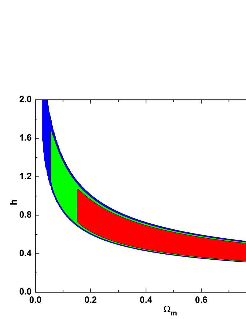
Figure 2: Confidence regions ($68.3$%, $95.4$% and $99.7$%) in the $(\Omega_{m},h)$ plane provided by Ly$\alpha$ forest data. The basic conclusion is that Ly$\alpha$ forest alone cannot constrain the pair of parameters.

Figure 3: Contours in the $\Omega_{m}-h$ plane provided by the joint analysis combinig Ly$\alpha$ Forest and BAO. As before, the contours correspond to $68.3$%, $95.4$% and $99.7$% confidence levels. Note that the best-fit model converges to $h=0.67$ and $\Omega_{m}=0.23$. These results should be compared with the ones presented in Figure 2.

Table 1: Limits to $H_{0}$

Method	Reference	h
Cepheid Variables	Freedman (2001) (HST Project)	$0.72\pm 0.08$
Age Redshift	Jimenez et al. (2003) (SDSS)	$0.69\pm 0.12$
SNe Ia/Cepheid	Sandage et al. (2006)	$0.62\pm 0.013$(rand.)$\pm 0.05$(syst.)
SZE+BAO	Cunha et al. (2007)	$0.74^{+0.04}_{-0.03}$
Old Galaxies + BAO	Lima et al. (2009)	$0.71\pm 0.04$
SNe Ia/Cepheid	Riess et al. (2009)	$0.742\pm 0.036$
CMB	Komatsu et al. (2011) (WMAP)	$0.710\pm 0.025$
SZE+BAO	Holanda et al. (2010)	$0.732^{+0.043}_{-0.037}$
Time-delay lenses	Paraficz & Hjorth (2010)	$0.76\pm 0.03$
Ly$\alpha$ + BAO	This work	$0.67^{+0.24}_{-0.09}$

References

- Amanullah et al. (2010) Amanullah, R., et al. 2010, ApJ, 716, 712
- Aracil et al. (2004) Aracil, B., Petitjean, P., Pichon, C., & Bergeron, J. 2004, A&A, 419, 811
- Bergeron et al. (2004) Bergeron, J., et al. 2004, The Messenger, 118, 40
- Bolton et al. (2005) Bolton, J. S., Haehnelt, M. G.,Viel, M., & Springel, V. 2005, MNRAS, 357, 1178
- Burles et al. (2001) Burles, S., Nollett, K. M., & Turner, M. S. 2001, ApJ, 552, 1
- Chand et al. (2004) Chand, H., Srianand, R., Petitjean, P., & Aracil, B., 2004, A&A, 417, 853
- Croft et al. (1998) Croft, R. A. C., Weinberg, D. H., Katz, N., & Hernquist, L. 1998, ApJ, 495, 44
- Croft et al. (1999) Croft, R. A. C., Weinberg, D. H., Pettini, M., Hernquist, L., & Katz, N. 1999, ApJ, 520, 1
- Cunha et al. (2007) Cunha, J. V., Marassi, L., & Lima, J. A. S. 2007, MNRAS, 379, L1
- Eisenstein (2005) Eisenstein, D. J., et al. 2005, ApJ, 633, 560
- Faucher-Giguère et al. (2008a) Faucher-Giguère, C.-A., Lidz, A., Hernquist, L, & Zaldarriaga, M., 2008a, ApJ, 682, 9
- Faucher-Giguère et al. (2008b) Faucher-Giguère, C.-A., Lidz, A., Hernquist, L, & Zaldarriaga, M., 2008b, ApJ, 688, 85
- Freedman (2001) Freedman, W. L., et al. 2001, ApJ, 553, 47
- Freedman & Madore (2010) Freedman, W. L., & Madore, B. F., 2010, ARA&A, 48, 673
- e.g., Gnedin & Hui (1998) Gnedin, N. Y., & Hui, L. 1998, MNRAS, 296, 44
- Guimarães et al. (2007) Guimarães, R., Petitjean, P., Rollinde, E., de Carvalho, R. R., Djorgovski, S. G., Srianand, R., Aghaee, S., & Castro, S. 2007, MNRAS, 377, 657
- Holanda et al. (2010) Holanda, R. F. L., Cunha, J. V., Marassi, L., & Lima, J. A. S., 2010, arXiv:1006.4200
- Hui & Gnedin (1997) Hui, L., & Gnedin, N. Y. 1997, MNRAS, 292, 27
- Hui (1999) Hui, L. 1999, ApJ, 516, 519
- Jackson (2007) Jackson, N. 2007, Living Rev. Relativ., 10, 4
- Jimenez et al. (2003) Jimenez, R., Verdi, L., Treu, T., & Stern D. 2003, ApJ, 593, 622
- Kirkman et al. (2005) Kirkman, D., et al. 2005, MNRAS, 360, 1373
- Komatsu et al. (2011) Komatsu, E., et al. 2011, ApJS, 192, 18
- Lima et al. (2009) Lima, J. A. S., Jesus, J. F., & Cunha, J. V. 2009, ApJ, 690, 85
- Mandelbaum et al. (2003) Mandelbaum, R., McDonald, P., Seljak, U., & Cen, R. 2003, MNRAS, 344, 776
- McDonald & Miralda-Escudé (2001) McDonald, P., & Miralda-Escudé, J. 2001, ApJ, 549, 11
- McDonald et al. (2000) McDonald, P., Miralda-Escudé, J., Rauch, M., Sargent, W. L. W., Barlow, T. A., Cen, R., & Ostriker, J. P. 2000, ApJ, 543, 1
- McDonald et al. (2005) McDonald, P., et al. 2005, ApJ, 635, 761
- Meiksin & White (2004) Meiksin, A., & White, M. 2004, MNRAS, 350, 1107
- Miralda-Escudé et al. (1996) Miralda-Escudé, J., Cen, R., Ostriker, J. P., & Rauch, M. 1996, ApJ, 471, 582
- Miralda-Escudé et al. (2000) Miralda-Escudé, J., Haehnelt, M., & Rees, M. J. 2000, ApJ, 530, 1
- Nusser & Haehnelt (1999) Nusser, A., & Haehnelt, M., 1999, MNRAS, 303, 179
- Padmanabhan (2002) Padmanabhan, T. 2002, Theoretical Astrophysics Volume III: Galaxies and Cosmology (Cambridge: Cambridge Univ. Press)
- Paraficz & Hjorth (2010) Paraficz, D., & Hjorth, J. 2010, ApJ, 712, 1378
- Peebles (1993) Peebles, P. J. E. 1993, Principles of Physical Cosmology (New Jersey: Princeton Univ. Press)
- Percival et al. (2010) Percival, W., et al. 2010, MNRAS, 401, 2148
- Pettini et al. (2008) Pettini, M., Zych, B. J., Murphy, M. T., Lewis, A., & Steidel, C. C. 2008, MNRAS, 391, 1499
- Prochaska et al. (2003a) Prochaska J. X., Gawiser E., Wolfe A., et al. 2003a, ApJ, 595, 9
- Prochaska et al. (2003b) Prochaska J. X., Castro S., & Djorgovski S. G., 2003b, ApJS, 148, 317
- Rauch et al. (1997) Rauch, M., et al., 1997 ApJ, 489, 7
- Riess et al. (2009) Riess, A. G., et al., 2009 ApJ, 699, 539
- Sandage et al. (2006) Sandage, A., Tammann, G. A., Saha, A., Reindl, B., Macchetto, F. D., & Panagia, N. 2006, ApJ, 653, 843
- Sheinis et al. (2002) Sheinis, A. I.,Bolte, M., Epps, H. W., et al. 2002, PASP, 114, 851
- Simha & Steigman (2008) Simha, V., & Steigman, G. 2008, J. Cosmology Astropart. Phys, 06, 16
- Tytler et al. (2004) Tytler, D., et al. 2004, ApJ, 617, 1
- Viel et al. (2009) Viel, M., Bolton, J. S., & Haehnelt, M. G. 2009, MNRAS, 399, L39
- Weinberg et al. (2003) Weinberg, D. H., Davé, R., Katz, N., & Kollmeier, J. A. 2003, in AIP Conf. Proc. 666, The Emergence of Cosmic Structure, ed. S. S. Holt, & C. S. Reynolds (New York: AIP), 157
- Wyithe et al. (2008) Wyithe, J. S. B., Bolton, J. S., & Haehnelt, M. G. 2008, MNRAS, 383, 691
- Zaldarriaga et al. (2001) Zaldarriaga, M., Hui, L., & Tegmark, M. 2001, ApJ, 557, 519