On the Anomalous Diffusion in Nonisothermal plasma

Abstract

In nonisothermal plasma at temperature $T_{e}>>T_{i}$ diffusion plays decisive role at conditions of smooth inhomogeneity when the inhomogeneity size is larger than the Debye radius by more than $\sqrt{T_{e}/T_{i}}$ times. When the inhomogeneity is rather abrupt and the condition is violated, then during the spreading process the Maxwellian relaxation of ion charges becomes significant. Here, we consider these two phenomena together and refer to the anomalous character of diffusion, i.e. anomalous diffusion.

I Introduction

One can talk of plasma as a continous medium when its size (and the inhomogenuity size) exceeds significantly the Debye radius. In a case of nonisothermal plasma $T_{e}>>T_{i}$ Debye radius is determined through the ion temperature and is equal to $v_{Ti}/\omega_{Li}$, where $v_{Ti}=\sqrt{T_{i}/M}$ is the ion thermal velocity and $\omega_{Li}=\sqrt{4\pi{q_{i}}^{2}n_{i0}/M}$ is the ion Langmur frequency with $q_{i}=Ze$ being the ion charge, $n_{i0}$ - equillibrium ion density ($en_{e0}=q_{i}n_{i0}$), here $e$ - electron charge. Here and below we use the CGS unit system. We write for general case but further on we present the results of our calculations only for the Hydrogen plasma Z=1.
The diffusion process is characterized through the mean square displacement dependence on time:

$$<r^{2}(t)>=\frac{\int r^{2}n(\vec{r},t)d\vec{r}}{\int n(\vec{r},t)d\vec{r}}\sim t^{\gamma},$$ (1)

If $\gamma=1$ then diffusion is termed as normal, in all other cases one refers to the anomalous character of diffusion: $\gamma>1$ - superdiffusion, $\gamma<1$- subdiffusion.
When the size of innhomogeneity of ionic component perturbation is larger than the Debye radius by more than $\sqrt{T_{e}/T_{i}}$ times, then spreading of the ionic component perturbation has a diffusive character and is defined by the time of the normal ambipolar diffusion Princpls . If it is less then the Maxwellian relaxation of ionic charges becomes dominant during the spreading of inhomogenuity Lasers ; Waves .
We will introduce a reader below into the theory of spreading of perturbation in nonisothermal plasma taking into account both mentioned phenomena and show the anomalous character of diffusion.

II Anomalous diffusion model

First of all, we will consider the main equations of the studied phenomenon and its constraints.
The main constraints for the considered below equations are:

$$\omega\nu_{i}>>\omega^{2};\>k^{2}v_{Te}^{2}>>\omega\nu_{e};\>\nu_{e}>>kv_{Te},\omega;\>\nu_{i}>>kv_{Ti},\omega$$ (2)

Here $\nu_{e}$, $\nu_{i}$ are electron-atom and ion-atom collision frequencies, $v_{Te}=\sqrt{T_{e}/m}$ - electron thermal velocity with $m$ being the electron mass. Nonisothermal plasma can be only the weakly ionized plasma, in which the dominant collisions are charged particle-atom, -molecule collisions, $\omega\propto 1/\tau$, where $\tau$ is the characteristic time of spreading and $k\propto 1/L$, where $L$ is the characteristic size of spreading.

• Equation of motion of electrons and ions has the following view:

  $$\frac{q_{i}\vec{E}}{M}-\nu_{i}\vec{v}_{i}=0,\>q_{e}\vec{E}-\frac{T_{e}}{n_{e}}\Delta n_{e}=0,$$ (3)

  Here $q_{e}=e$, $q_{i}=Ze$ are the electron and ion charges, $Z\leq|q_{i}/q|$, $\vec{E}$ are the self-consistent field, $\vec{v}_{i}$, $\vec{v}_{e}$ are ion and electron velocities, $T_{i}=0$, $T_{e}=const$, $n_{i}$, $n_{e}$ are the ion and electron densities.

• Field equation (Poisson equation)

  $$div\vec{E}=4\pi e(n_{e}-Zn_{i})$$ (4)

• Continuity equation of the ion component

  $$\frac{\partial n_{i}}{\partial t}+div\>n_{i}\vec{v}_{i}=0$$ (5)

• Equilibrium state satisfying the stationary equations (3)-(5) at $\vec{E}_{0}=0$ takes the following view:

  $$q_{e}n_{e0}=q_{i}n_{i0}=Zen_{i0}=Const$$ (6)

  Let’s consider the small density perturbations :

  $$n_{e}=n_{e0}+\delta n_{e},\>n_{i}=n_{i0}+\delta n_{i},$$ (7)

  where $n_{\alpha 0}$ - denity of the homogenious background. These small density perturbations lead to the emergence of the weak self-consistent field $\vec{E}$.
  

System of equations (3)-(5) at (6) for small perturbations (7) can be deduced to one equation for perturbation $\delta n_{i}$. The rest magnitudes can be expressed through $\delta n_{i}$. Equation for $\delta n_{i}$ has the following view:

$$({\omega_{Li}}^{2}-{v_{S}}^{2}\Delta)\frac{\partial\delta n_{i}}{\partial t}-\frac{{v_{S}}^{2}}{\nu_{i}}{\omega_{Li}}^{2}\Delta\delta n_{i}=0.$$ (8)

Here $\omega_{Li}$ is the equlibrium Langmuir ion frequency, ${v_{S}}^{2}=ZT_{e}/M$ is the squared ion sound velocity and $\nu_{i}=Const$. Eq. (8) represents the partial differential equation of the first order with the constant coefficients.
Let us formulate the Koshi problem for Eq. (8), i.e. we consider infinite plasma and set the following initial condition:

$$\delta n_{i}(\vec{r},0)=f(\vec{r}),$$ (9)

and take into account that $lim_{r\to\infty}\delta n_{i}=0$. Using the Fourier transform

$$\begin{gathered}\delta n_{i}(\vec{r},t)=\int d\vec{k}\delta n_{i}(\vec{k},t)\exp(i\vec{k}\cdot\vec{r}),\hfill\\ f(\vec{k})=\frac{1}{(2\pi)^{3}}\int d\vec{r}f(\vec{r})\exp(-i\vec{k}\cdot\vec{r}),\end{gathered}$$ (10)

Eq. (8) will be reduced to the ordinary differential equation of the first time order.

$$\frac{\partial\delta n_{i}(\vec{k},t)}{\partial t}=-\frac{k^{2}{\omega_{Li}}^{2}{v_{S}}^{2}/\nu_{i}}{{\omega_{Li}}^{2}+k^{2}{v_{S}}^{2}}\delta n_{i}(\vec{k},t).$$ (11)

We obtain the solution of Eq. (11) with the initial condition

$$\delta n_{i}(\vec{k},0)=f(\vec{k}),$$

as following:

$$\delta n_{i}(\vec{k},t)=f(\vec{k})\exp\left(-t\frac{k^{2}{\omega_{Li}}^{2}{v_{S}}^{2}/\nu_{i}}{{\omega_{Li}}^{2}+k^{2}{v_{S}}^{2}}\right).$$ (12)

Making the inverse Fourier transform (10), we can find

$$\delta n_{i}(\vec{r},t)=\int d\vec{k}f(\vec{k})\exp\left(i\vec{k}\cdot\vec{r}-t\frac{k^{2}{\omega_{Li}}^{2}{v_{S}}^{2}/\nu_{i}}{{\omega_{Li}}^{2}+k^{2}{v_{S}}^{2}}\right).$$ (13)

Let us analyse the limitting cases of Eq. (13).

• . In a case of rare plasma, when ${\omega_{Li}}\to 0$:

  $$\delta n_{i}(\vec{r},t)= \int d\vec{k}f(\vec{k})\exp\left(i\vec{k}\cdot\vec{r}-t\frac{{\omega_{Li}}^{2}}{{\nu_{i}}}\right)$$ (14)

  $$=f(\vec{r})\exp\left(-t\frac{{\omega_{Li}}^{2}}{{\nu_{i}}}\right).$$

  This solution corresponds to the Maxwellian temporary relaxation of the charge density perturbation.

• . In a case of dense plasma, when ${\omega_{Li}}^{2}>>k^{2}{v_{S}}^{2}$:

  $$\delta n_{i}(\vec{r},t)=\int d\vec{k}f(\vec{k})\exp\left(i\vec{k}\cdot\vec{r}-t\frac{k^{2}{v_{S}}^{2}}{\nu_{i}}\right).$$ (15)

  The integral can be easily solved at Eq. (9), when $f(\vec{r})=N_{i0}\delta(\vec{r})$ with the corresponding Fourier transform $f(\vec{k})=\frac{N_{i0}}{(2\pi)^{3}}$, where $N_{i0}$ is the total number of perturbed particles at $r=0$. The result is well known Lan :

  $$\delta n_{i}(\vec{r},t)=\frac{N_{i0}}{8(\pi Dt)^{3/2}}\exp\left(-r^{2}/4Dt\right),$$ (16)

  where $D={v_{S}}^{2}/\nu_{i}$ is the coefficient of ambipolar difusion and Eq. (16) describes the diffusive spreading of the localized ion density perturbation ($\delta$ - functional).
  Let us determine the $<r^{2}(t)>$ Eq. (1) for the ambipolar diffusion (16):

  $$<r^{2}(t)>=6Dt,$$ (17)

  here in Eq. (1) we used $\delta n_{i}$ Eq. (18). As one can see this corresponds to the normal diffusion.

Let us choose the following two initial perturbations $f(\vec{r})$, the first as representing the infinite wave:

$$f(\vec{r})=n_{i0}\cos(\vec{r}\cdot\vec{k}_{0})$$ (18)

with the Fourier transform $f(\vec{k})=\frac{\delta(\vec{k}-\vec{k}_{0})+\delta(\vec{k}+\vec{k}_{0})}{2}$, here $\vec{k}_{0}$ is the wave vector; and the second as repesenting the localized ion density perurbation mentioned above:

$$f(\vec{r})=N_{i0}\delta(\vec{r})$$ (19)

with the Fourier transform $f(\vec{k})=\frac{N_{i0}}{(2\pi)^{3}}$, what will be discussed later. We would lik to start with the condition (18).
Then, the equation (14) corresponding to the Maxwell relaxation will turn into

$$\delta n_{i}(\vec{r},t)=n_{i0}\exp\left(-\frac{\omega_{Li}^{2}t}{\nu_{i}}\right)\cos(\vec{r}\cdot\vec{k}_{0})$$

or in dimensionless form

$$\frac{\delta n_{i}(\vec{R},T)}{n_{i0}}=\exp\left(-\frac{\omega_{Li}T}{\nu_{i}}\right)\cos(\vec{R}\cdot\vec{e}_{0}),$$ (20)

here , $\vec{k}_{0}r_{D}=\vec{e}_{0}$, $R=r/r_{D}$, $T=t\omega_{Li}$ - dimensionless time.
The equation (15) corresponding to the ambipolar diffusion will turn into

$$\delta n_{i}(\vec{r},t)=n_{i0}\exp\left(-\frac{k_{0}^{2}v_{S}^{2}t}{\nu_{i}}\right)\cos(\vec{r}\cdot\vec{k}_{0})$$

or in dimensionless form

$$\frac{\delta n_{i}(\vec{R},T)}{n_{i0}}=\exp\left(-\frac{k_{0}^{2}DT}{\omega_{Li}}\right)\cos(\vec{R}\cdot\vec{e}_{0}),$$ (21)

here $\vec{k}_{0}$ is the same wave vector.
Finally, the equation for anomalous diffusion (13) will become

$$\delta n_{i}(\vec{r},t)=n_{i0}\exp\left(-t\frac{k_{0}^{2}D{\omega_{Li}}^{2}{v_{S}}^{2}}{{\omega_{Li}}^{2}+k_{0}^{2}{v_{S}}^{2}}\right)\cos(\vec{r}\cdot\vec{k}_{0}).$$

or in dimensionless form

$$\frac{\delta n_{i}(\vec{R},T)}{n_{i0}}=\exp\left(-t\frac{k_{0}^{2}D{\omega_{Li}}{v_{S}}^{2}}{{\omega_{Li}}^{2}+k_{0}^{2}{v_{S}}^{2}}\right)\cos(\vec{R}\cdot\vec{e}_{0}).$$ (22)

As one can easily see in all cases, Eqs. (20)-(22), the functions get separated by variables $T$ and $R$. As a result we can not define the mean square displacement. This means that at the given oscillatory initial perturbaion (18) no normal diffusion occurs: the initial perturbation gets faded down with the time evolution keeping its initial functional form in space - $\cos(\beta R)$, i.e. only the amplitude decreases. This behaviour is peculiar for the Maxwellian relaxation (14) independent on the type of initial condition. However, when we take another initial condition ($\delta(\vec{r})$ - functional) for the case of diffusive relaxation (15) then we obtain the normal ambipolar diffusion (16).
Finally, let us find the solution for the anomalous diffusion Eq. (13) with the second initial condition Eq. (19) as representing the localized ion charge perturbation. Having solved this equation and having made some simplifications, we have got the following:

$$\frac{\delta n_{i}(r,t)}{N_{i0}/r_{D}^{3}} = \frac{r_{D}^{3}}{(2\pi)^{3}}\int d\vec{k}\exp\left(i\vec{k}\cdot\vec{r}-t\frac{k^{2}{\omega_{Li}}^{2}{v_{S}}^{2}/\nu_{i}}{{\omega_{Li}}^{2}+k^{2}{v_{S}}^{2}}\right)$$ (23)

$$= \frac{r_{D}^{3}}{2\pi^{2}}\int_{0}^{10\omega_{Li}/v_{s}}dkf(k)k\frac{\sin(kr)}{r}$$

$$\times \exp\left(-t\frac{k^{2}v_{s}^{2}\omega_{Li}^{2}/\nu_{i}}{\omega_{Li}^{2}+k^{2}v_{s}^{2}}\right)+\delta(\vec{r})r_{D}^{3}\exp\left(-t\frac{\omega_{Li}^{2}}{\nu_{i}}\right)$$

$$- \frac{r_{D}^{3}}{2\pi^{2}}\exp\left(-t\frac{\omega_{Li}^{2}}{\nu_{i}}\right)\int_{0}^{10\omega_{Li}/v_{s}}dkk\frac{\sin(kr)}{r}$$

III Results and Discussions

In the Figure 1 a) the 3 dimensional view of the relative value of density perturbation in dependence on time $T$ and absolute value of the radius vector $R$ is shown. Namely, Fig. 1 a) represents the anomalous relaxation as the combined effect Eq. (22) of the Maxwellian relaxation Eq. (20) and ambipolar diffusive relaxation Eq. (21). In Fig. 1 b) the comparison among the mentioned relaxations and the localized ion density perturbation relaxation Eq. (16) at $t=1/\omega_{Li}$ is shown.
As one can easily see the behaviour of the Maxwellian relaxation Eq. (20), ambipolar diffusive relaxation Eq. (21), and the anomalous diffusion Eq. (16) is oscillatory and fades down with the time as the $\exp(-\alpha t)\cos(\beta R)$ function. In a case for the localized ion density perturbation relaxation Eq. (16) the perturbations fades down as the $\exp(-\gamma R^{2}/t)/t^{3/2}$.
At the given oscillatory initial perturbation (18) no normal diffusion occurs: the initial perturbation gets faded down with the time evolution keeping its initial spatial functional form - $\cos(\beta R)$, i.e. only the amplitude decreases, and in this way revealing the anomalous nature of the diffusion in nonisothermal plasma. This behaviour is peculiar for the Maxwellian relaxation (14) independent on the type of initial condition. However, when we take another initial condition ($\delta(\vec{r})$ - functional) for the case of diffusive relaxation (15) then we obtain the normal ambipolar diffusion (16).
In the Figures 2, 3, 4, and 5 comparison between the obtained relative density perturbation relaxation for anomalous diffusion Eq. (23) with $\delta(\vec{r})$ as initial perturbation (19) and normal ambipolar diffusion Eq. (16) and corresponding variances at the different ion Langmuir frequencies and different time moments are shown. In the Figs. 2, 3 the difference between the obtained curves for anomalous diffusion and the normal ambiplar diffusion is quite significant, whereas with an increase of either ion Langmuir frequency or time the anomalous diffusion gets to turn into the normal ambipolar diffusion. This is also demonstrated in the correspoding Figs.  d) where dependence of the variance on time and the fitting curves for the corresponding different Langmuir frequencies is shown. The variance was estimated using Eq. (1). As we can see at the lowest frequency there is almost no diffusion Fig. 2 d), the variance does not depend on time. However, with further increase of the ion frequency the diffusion becomes anomalous $<r^{2}(t)>\neq\alpha t$ ($\alpha$=Const), whereas when the frequency and time moments increase the diffusion starts to turn into the normal: $<r^{2}(t)>=\alpha t$ (17).

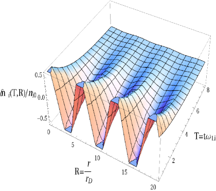
a)

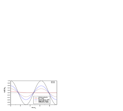
b)

Figure 1: a) The anomalous diffusion Eq. (22) and b) comparison among the anomalous, Maxwellian relaxation Eq. (20), ambipolar diffusive relaxation Eq. (21) and the localized ion density perturbation relaxation Eq. (16) at $t=1/\omega_{Li}$ is shown. Here, $\vec{e}_{0}||\vec{R}$, $T_{e}=10$ eV, $n_{i0}=10^{12}cm^{-3}$, $\omega_{Li}=1.3\cdot 10^{9}s^{-1}$, $\nu_{i}=1.2\cdot 10^{9}s^{-1}$, $n_{0}=3\cdot 10^{16}cm^{-3}$ (atom density), $r_{D}=2.3\cdot 10^{-5}m$.

a)

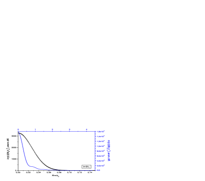
b)

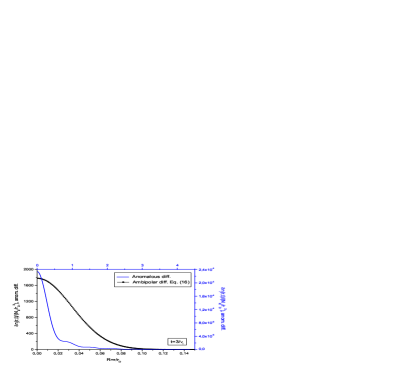
c)

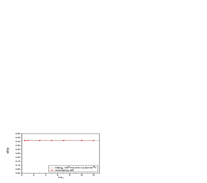
d)

Figure 2: Comparison between the obtained the relative density perturbation relaxation for anomalous diffusion Eq. (23) and normal ambipolar diffusion Eq. (16) at the different time moments $T=t\nu_{i}$ but fixed Langmuir frequency $\omega_{Li}=1.6\cdot 10^{7}$ s^-1, $n_{i0}=1.5\cdot 10^{8}$ cm^-3 and its variance Eq. (1) together with the variance fit d) are shown. Here $T_{e}=10$ eV, $\nu_{i}=1.2\cdot 10^{9}$ s^-1, $n_{0}=3\cdot 10^{16}$ cm^-3 (atom density).

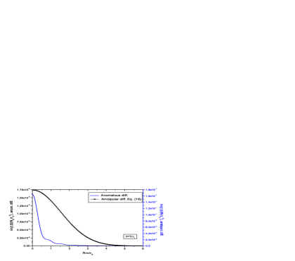
a)

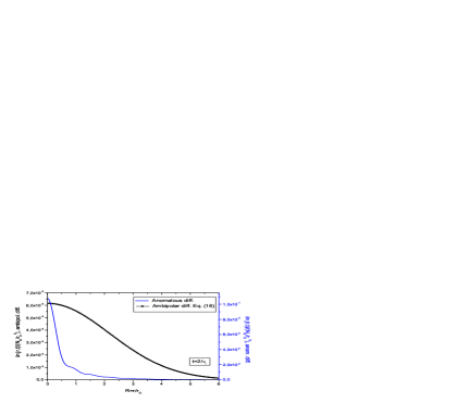
b)

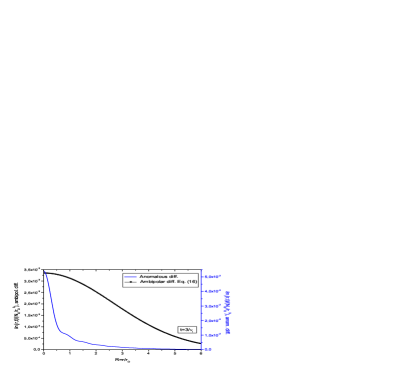
c)

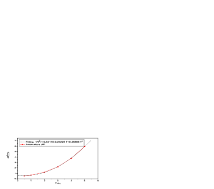
d)

Figure 3: Comparison between the obtained the relative density perturbation relaxation for anomalous diffusion Eq. (23) and normal ambipolar diffusion Eq. (16) at the different time moments $T=t\nu_{i}$ but fixed Langmuir frequency $\omega_{Li}=1.3\cdot 10^{9}s^{-1}$, $n_{i0}=10^{12}$ cm^-3 and its variance Eq. (1) together with the variance fit d) are shown. The Hydrogen plasma parameters are the same as in the Fig. 2.

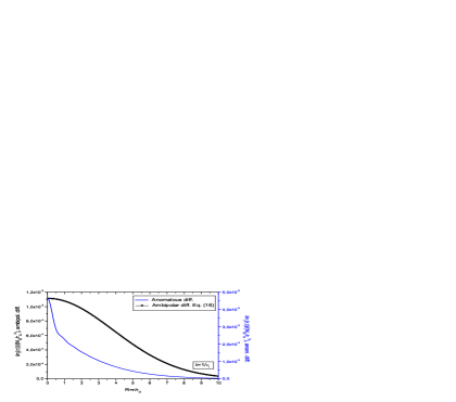
a)

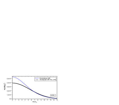
b)

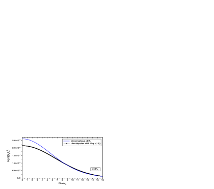
c)

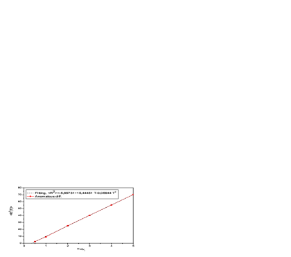
d)

Figure 4: Comparison between the obtained the relative density perturbation relaxation for anomalous diffusion Eq. (23) and normal ambipolar diffusion Eq. (16) at the different time moments $T=t\nu_{i}$ but fixed Langmuir frequency $\omega_{Li}=3.3\cdot 10^{9}$ s^-1, $n_{i0}=6.25\cdot 10^{12}$ cm^-3 and its variance Eq. (1) together with the variance fit d) are shown. The Hydrogen plasma parameters are the same as in the Fig. 2.

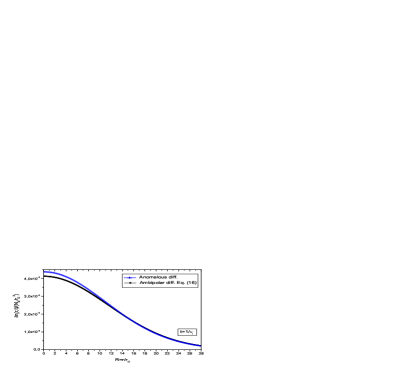
a)

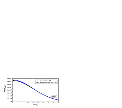
b)

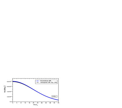
c)

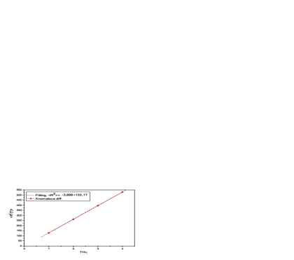
d)

Figure 5: Comparison between the obtained the relative density perturbation relaxation for anomalous diffusion Eq. (23) and normal ambipolar diffusion Eq. (16) at the different time moments $T=t\nu_{i}$ but fixed Langmuir frequency $\omega_{Li}=9.7\cdot 10^{9}$ s^-1, $n_{i0}=5.6\cdot 10^{13}$ cm^-3 and its variance Eq. (1) together with the variance fit d) are shown. The Hydrogen plasma parameters are the same as in the Fig. 2

References

• (1) A.F. Alexandrov, L.S. Bogdankevich, A.A.Rukhadze, in Priciples of Plasma Elektrodynamics, Springer Series in Electrophysics, Volume 9, edited by G. Ecker (Ruhr-Universit t Bochum) (Springer-Verlag, Berlin, Heidelberg, New York, Tokio, 1984).
• (2) M.V. Kuzelev A.A, Rukhadze, in Basic of Plasma Free Elektron Lasers (Edition frontier, Paris, 1995).
• (3) M.V. Kuzelev A.A, Rukhadze, in Methods of wave theory in dispersive media (World Scientic Publishing, Singapore, 2010)
• (4) L.D. Landau, E.M. Lufshitz, in Hydrodynamics (Nauka, Moscow, 1982)