The origin of the early time optical emission of Swift GRB 080310

Abstract

We present broadband multi-wavelength observations of GRB 080310 at redshift $z$ $=$ $2.43$. This burst was bright and long-lived, and unusual in having extensive optical and near IR follow-up during the prompt phase. Using these data we attempt to simultaneously model the $\gamma$-ray, X-ray, optical and IR emission using a series of prompt pulses and an afterglow component. Initial attempts to extrapolate the high energy model directly to lower energies for each pulse reveal that a spectral break is required between the optical regime and 0.3 keV to avoid over predicting the optical flux. We demonstrate that afterglow emission alone is insufficient to describe all morphology seen in the optical and IR data. Allowing the prompt component to dominate the early-time optical and IR and permitting each pulse to have an independent low energy spectral indices we produce an alternative scenario which better describes the optical light curve. This, however, does not describe the spectral shape of GRB 080310 at early times. The fit statistics for the prompt and afterglow dominated models are nearly identical making it difficult to favour either. However one enduring result is that both models require a low energy spectral index consistent with self absorption for at least some of the pulses identified in the high energy emission model.

1 Introduction

Over the last few years a combination of fast-response ground-based telescopes triggered by the availability of rapid, accurate localisations have started to provide the data required to answer the question of what is causing the early, bright X-ray and optical emission from gamma-ray bursts (GRBs). The most accurate prompt X-ray locations come from the Swift satellite (Gehrels et al., 2004). These are supplemented by either on-board or ground detections of the ultraviolet (UV), optical or infra-red (IR) counterpart.

In the popular relativistic fireball model for GRBs, the early, usually highly variable emission is understood to be due to internal shocks (Sari & Piran, 1997) or magnetic dissipation within the jet, and the so-called $external$ emission is produced by the interaction of the jet with the surrounding medium. The latter emission is usually described using the fireball model (Rees & Meszaros, 1992), which has successfully been applied to describe the behaviour of GRBs half a day or so after the trigger, but has difficulties explaining the complex behaviour seen in the first few hours, a period now routinely accessed by Swift and other rapid-response facilities. Ideally multi-wavelength observations should be obtained while the burst is happening so as to try to disentangle the relative contribution from the internal and external components.

Evans et al. (2009) present a uniformly analysed comprehensive sample of 317 Swift GRBs spanning from December 2004 to July 2008, in which their morphologies are compared to the proposed canonical X-ray light curve (Nousek et al. 2006, Zhang et al. 2006 & Panaitescu et al. 2006). Such canonical light curves consider the X-ray emission to consist of a series of power-laws, where one important phase is the rapid decay phase which has been explained as being the smooth continuation of the prompt emission (O’Brien et al. 2006, Tagliaferri et al. 2005 & Barthelmy et al. 2005). From the sample of Evans et al. (2009) it is clear that the X-ray light curves of GRBs vary from burst to burst. Some show strong flaring, one example being GRB 061121 (Page et al., 2007), however, some bursts show remarkably simple and smooth decay (GRB 061007; Schady et al. 2007). Similar findings are also reported in Racusin et al. (2009). Rapid behaviour, such as flaring, at high energies is often attributed to central-engine behaviour (Margutti et al., 2010) but how this relates to the optical emission remains somewhat of a mystery. The available datasets reveal a confusing picture. In some cases the early optical data seem to trace the X-ray and $\gamma$-ray light curves, such as GRB 041219A (Vestrand et al. 2005 & Blake et al. 2005), suggesting that optical flaring may be of internal origin. In other GRBs the optical behaviour seems entirely unrelated to the the high-energy emission (GRB 990123; Akerlof et al. 1999 & GRB 060607A; Nysewander et al. 2009 & Molinari et al. 2007), and instead seems to follow the behaviour of the external afterglow.

To make progress requires continued efforts to observe GRBs over as wide a wavelength range as possible from as early as possible. This is only really viable for bright, long-lasting GRBs which are well-placed for rapid follow-up. Here we present prompt, multi-wavelength data from the GRB 080310, which begin at a time soon after the trigger that is not often accessed by ground-based facilities. Following the trigger, GRB 080310 was detected on-board Swift by both the X-Ray Telescope (XRT) (Burrows et al., 2005) and UV/Optical Telescope (UVOT) (Roming et al., 2005) and also observed in the optical and IR by several ground-based telescopes. These rare data present us with an opportunity to discriminate between whether the early time lower-energy light curve of a GRB is driven by internal or external emission, during which time the high-energy emission is presumed to be totally internally dominated.

In the following section we discuss the observations, then in §3 we present attempts to fit both an internal shock model (Genet & Granot, 2009) and an afterglow component (Willingale et al., 2007) to the X-ray and $\gamma$-ray data, and describe the necessary modification required to simultaneously fit the early optical emission in two scenarios, where either the prompt or afterglow components dominate this early flux. In §4 we briefly discuss the relative merits of using each component, before finally in §5 we conclude which of the two alternatives is a better fit to the observed data and consider the implications of the model on the physics governing the emission from GRB 080310.

2 Observations

On 2008 March 10 the Swift BAT triggered and located GRB 080310 (trigger number 305288) on board at 08:37:58 UT (Cummings et al., 2008). Swift slewed immediately which enabled the narrow field instruments to begin observing the burst $89{\rm\thinspace s}$ after the trigger. The burst was detected by the XRT and UVOT (white filter), with the latter providing the best Swift position of ${\rm RA(J2000)}=14^{h}40^{m}13\aas@@fstack{s}80$, ${\rm Dec(J2000)}=-00\degr 10\arcmin 29\aas@@fstack{\prime\prime}6$ with a 1$\sigma$ error radius of $0\aas@@fstack{\prime\prime}6$. Figure 1 shows a UVOT $v$-band image from the early time data. The Swift light curves obtained in multiple bands from each of the three on board instruments are presented in Figure 2 and most of the available datasets from an extensive number of facilities are shown in Figure 3. Data from the PAIRITEL (Perley et al., 2008) and KAIT instruments are shown separately in Figure 4.

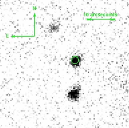
Figure 1: UVOT $v$-band image from $T_{0}+79{\rm\thinspace s}$ to $T_{0}+1539{\rm\thinspace s}$. The enhanced Swift XRT position is shown (Osborne et al., 2008), with an error circle of radius $1\aas@@fstack{\prime\prime}4$, corresponding to the 90% confidence limit, containing the optical afterglow candidate at an average $v$-band magnitude of 17.49.

In addition to Swift observations, and those instruments already mentioned, GRB 080310 was also observed on the ground with numerous optical and NIR facilities, including REM (Covino et al., 2008), VLT (Covino et al., 2008) and the Faulkes Telescope North. These observations are shown alongside the BAT and XRT light curves in Figure 3.

The Kast dual spectrometer at the Lick Observatory, California, obtained the first redshift estimation for this burst of $z$ = 2.4266 (Prochaska et al., 2008) using strong absorption features from Silicon, Carbon and Aluminium. This was later corroborated by the VLT-UVES instrument (Vreeswijk et al., 2008) and the Keck-DEIMOS spectrometer (Prochaska et al., 2008).

The following subsections describe the observations in more detail. The Swift data analysis was performed using release 2.8 of the Swift software tools. Parameter uncertainties are estimated at the 90% confidence level. We note that the optical datasets have been reduced using different methods, and fully investigated the effects of cross calibration errors, ensuring that our later analysis remained insensitive to their effects.

2.1 BAT

The BAT data were processed using the standard batgrbproduct script. The top four panels of Figure 2 show the BAT light curves displayed in the standard energy bands of $15-25\thinspace\rm{keV}$, $25-50\thinspace\rm{keV}$, $50-100\thinspace\rm{keV}$ and $100-150\thinspace\rm{keV}$, plotted with respect to the BAT trigger time ($T_{0}$). The binning is such that each bin satisfies a minimum signal-to-noise ratio of 5 and a minimum time bin size of $1{\rm\thinspace s}$.

The $\gamma$-ray light curve shows many peaks with the first at $T_{0}-60{\rm\thinspace s}$. The brightest peak extends from $T_{0}-12{\rm\thinspace s}$ to $T_{0}+7{\rm\thinspace s}$. This is followed by a period of no detectable emission before a weaker, broad series of peaks is seen from $T_{0}+180{\rm\thinspace s}$ to $T_{0}+360{\rm\thinspace s}$ (Tueller et al., 2008). The latter peak is consistent with the first strong flare seen in the XRT (see below). The BAT emission is strongest in the lower energy bands, below $\sim 100\thinspace\rm{keV}$. The $T_{90}$ is estimated to be $365\pm 20{\rm\thinspace s}$ (where the error includes systematics).

The total spectrum from $T_{0}-71.76{\rm\thinspace s}$ to $T_{0}+318.75{\rm\thinspace s}$ is well fit by a power-law of photon index $2.32\pm 0.16$, with a total fluence of $2.3\pm 0.2\times 10^{-6}{\rm{\rm\thinspace erg}{\rm\thinspace cm}^{-2}}$ over the $15-150\thinspace\rm{keV}$ band. The fluence ratio $S(25-50\thinspace\rm{keV})/S(50-100\thinspace\rm{keV})$ is $1.27\pm 0.17$ which puts GRB 080310 on the border of the X-ray-rich gamma-ray bursts and X-ray flash (XRF) according to the definition of Sakamoto et al. (2008).

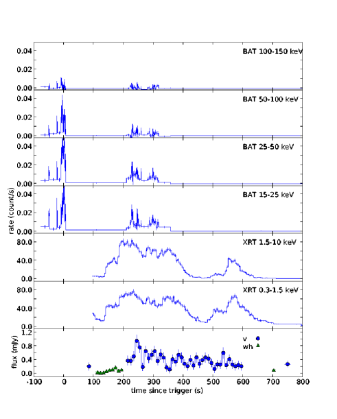
Figure 2: Swift prompt light curves from GRB 080310 in different energy bands. From top to bottom, BAT $100-150\thinspace\rm{keV}$, BAT $50-100\thinspace\rm{keV}$, BAT $25-50\thinspace\rm{keV}$, BAT $15-25\thinspace\rm{keV}$, XRT $1.5-10.0\thinspace\rm{keV}$, XRT $0.3-1.5\thinspace\rm{keV}$ and UVOT $v$ and white bands. Strictly, the count rates for BAT are per fully illuminated detector.

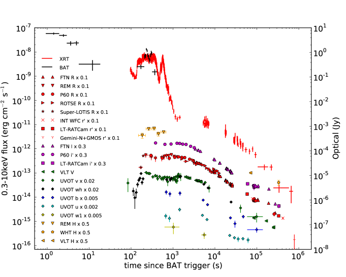
Figure 3: $\gamma$-ray to near IR light curves for GRB 080310, showing the energy bands used to observe the GRB and the instruments used to take the measurements. Data have been scaled from their actual values for viewing purposes.

2.2 XRT

The Swift XRT started observations of GRB 080310 $89{\rm\thinspace s}$ after the trigger, with windowed timing data ranging from $T_{0}+95{\rm\thinspace s}$ to $T_{0}+799{\rm\thinspace s}$ and photon counting mode data after this (Beardmore et al., 2008). As can be seen in Figure 2 the soft band XRT light curve initial fades until $T_{0}+130{\rm\thinspace s}$, before the burst rebrightens. This flaring activity continues until $T_{0}+420{\rm\thinspace s}$ before the count rate drops again briefly. A further flaring event is seen between $T_{0}+500{\rm\thinspace s}$ and $T_{0}+620{\rm\thinspace s}$, which is approximately half as bright as the first. There is significant spectral evolution during the flaring events, where the $S(1.5-10\thinspace\rm{keV})/S(0.3-1.5\thinspace\rm{keV})$ ratio shows a hardening in the spectrum at $T_{0}+135{\rm\thinspace s}$ to $T_{0}+200{\rm\thinspace s}$ and $T_{0}+500{\rm\thinspace s}$ to $T_{0}+565{\rm\thinspace s}$ before, in both instances, there is a softening as the flaring behaviour declines.

2.3 UVOT

UVOT observations began with a 100 second finding chart exposure taken at $T_{0}+99{\rm\thinspace s}$ (Hoversten & Cummings, 2008). This finding chart exposure was the sum of 10 individual 10 second exposures, with GRB 080310 being detected in all but the first exposure. At the time of GRB 080310 UVOT observations during the first orbit were taken in the event mode, which allows for higher timing resolution, while during subsequent orbits observations were taken in imaging mode. UVOT photometry was done using the publicly available FTOOLS data reduction suite, and is in the UVOT photometric system described in Poole et al. (2008). During the first 1,000 seconds the light curve is complex as shown in Figure 2, after which the the burst can be seen to fade in all the observed optical bands (Figure 3).

There are available data for the UVOT $white$, $v$, $b$, $u$ and $uvw1$. As this burst has a measured redshift of $z~{}=~{}2.43$ it is important to consider absorption from the intervening medium through which the emission must travel. Correction factors were calculated for Lyman absorption using the $GRBz$ code described in Curran et al. (2008). $GRBz$ uses the model presented by Madau (1995) to calculate the absorption from neutral Hydrogen in the intergalactic medium. Having found the correction factor for all the optical and near infrared bands presented in this work, we noted that it was only necessary to correct the data in the $b$, $u$ and $uvw1$ bands. Whilst the correction to both the $u$ and $b$ bands was not large, we found that the $uvw1$ data required a significant correction, within which there was a large uncertainty. Given that there were only two data points from UVOT in this band, we decided to remove them from any further analysis.

2.4 Faulkes Telescope North

Observations with the Faulkes Telescope North (FTN) started at 2008-03-10 09:31:07.3 (UT), 3.188 ks after the trigger. Data were reduced in a standard fashion using iraf (Tody, 1986). Calibration was performed using the SDSS data for the region (Adelman-McCarthy et al., 2007). For the $I$ and $R$ filters, the SDSS photometry was converted to the Johnson-Cousins system. Photometry was then performed using an aperture matched to the average seeing of the (combined) frames. For the conversion from magnitude to flux, the data were first corrected for Galactic extinction using the COBE-DIRBE extinction maps from Schlegel et al. (1998), and then converted using flux zero points from Fukugita et al. (1995) for optical and Tokunaga & Vacca (2005) for infrared. AB magnitudes were converted following Oke & Gunn (1983).

2.5 ROTSE

ROTSE-IIIb, located at McDonald Observatory, Texas, responded to GRB 080310 and began imaging 5.7 seconds after the GCN notice time (Yuan et al., 2008). Observations were carried out under fluctuating weather conditions. The optical transient (OT) was detected between 25 minutes and 3.5 hours after the trigger. To improve detection signal to noise ratio, sets of 4 to 11 images are co-added and exposures badly affected by weather are excluded. The OT is slightly blended with two nearby stars in the ROTSE images. We therefore subtract the scaled point spread functions (PSFs) of these two nearby stars and then apply PSF-matching photometry on the OT using our custom RPHOT package (Quimby et al., 2006). The analysis is further complicated by large seeing variation, particularly towards the end of the observation. The structure seen in the light curve during this time is likely not significant. The ROTSE-III unfiltered magnitudes are calibrated to SDSS $r$ using standard stars in the pre-burst SDSS observations (Cool et al., 2008).

2.6 REM

Early time optical and NIR data were collected using the 60-cm robotic telescope REM (Zerbi et al. 2001; Covino et al. 2004) located at the European Southern Observatory (ESO) La Silla observatory (Chile). The telescope simultaneously feeds, by means of a dichroic, the two focal instruments: REMIR (Conconi et al., 2004) a NIR camera, operating in the range 1.0 to 2.3 $\mu$m ($z^{\prime}$, $J$, $H$ and $K$) and ROSS (REM Optical Slitless Spectrograph; Tosti et al. 2004) an optical imager with spectroscopic (slitless) and photometric capabilities ($V$, $R$, $I$). Both cameras have a field of view of 10 $\times$ 10 arcmin².

REM reacted automatically after receiving the Swift alert for GRB 080310, and began observing about 150 seconds after the GRB trigger time (Covino et al., 2008).

Optical and NIR data were reduced following standard procedures. In particular, each single NIR observation with REMIR was performed with a dithering sequence of five images shifted by a few arcseconds. These images are automatically elaborated using the proprietary routine AQuA (Testa et al., 2004). The script aligns the images and co-adds all the frames to obtain one average image for each sequence. Astrometry was performed using USNO-B1 and 2MASS catalogue reference stars.

Photometry was derived by a combination of the SExtractor package (Bertin & Arnouts, 1996) and the photometric tools provided by the gaia package. The photometric calibration for the NIR was accomplished by applying average magnitude shifts computed using 2MASS isolated and non-saturated stars. The optical data were calibrated using instrumental zero points and checked with observations of standard stars in the field provided by Henden (2008).

2.7 VLT

VLT FORS1 $V$ and $R$ observations for GRB 080310 were automatically activated with the RRM mode allowing the telescope to react promptly to any alert. The field was acquired and the observations began less than seven minutes after the GRB trigger. Later VLT observations were obtained with ISAAC at about one day after the burst with the $J$, $H$ and $K$ filters. In addition linear polarimetry observations were carried out with FORS1 with the $V$ filter at approximately one, two and three days after the trigger.

Optical and NIR data were reduced following standard procedures with the tools of the ESO-eclipse package (Devillard, 1997). Polarimetric data were reduced again following standard procedures as discussed in Covino et al. (1999, 2002, 2003). Photometry was performed by means of the tools provided by the gaia package and with PSF photometry with the ESO-midas DAOPHOT context (Stetson, 1987).

The photometric calibration for the NIR was accomplished by applying average magnitude shifts computed using 2MASS isolated and non-saturated stars. The optical data were calibrated using instrumental zero points and checked with observations of standard stars in the field provided by Henden (2008). Linear polarimetry position angle was corrected by means of observations of polarimetric standard stars in the NGC 2024 region.

2.8 WHT

Late imaging was obtained with the 4.2m William Herschel Telescope (WHT), at Roque de los Muchachos Observatory (La Palma, Spain) using the Long-slit Intermediate Resolution Infrared Spectrograph (LIRIS) in its imaging mode. Observations consisted of $36\times 25$ second exposures in $H$-band, obtained on the 14th March 2008 from 04:36:28 to 04:53:41 UT. The data were reduced following standard procedures in iraf. For the photometric calibration, we used stars from the 2MASS catalogue as reference.

2.9 PAIRITEL

PAIRITEL (Bloom et al., 2006) responded to GRB 080310 and began taking data at 09:04:58 (UT) in the $J$, $H$, and $K$ filters simultaneously (Perley et al., 2008). The afterglow (Chornock et al., 2008) was well-detected in all three filters. Perley et al. (2008) also report on an SED constructed using data from PAIRITEL, KAIT and UVOT (Hoversten & Cummings, 2008), allowing a joint fit to be made and the estimation of a small amount ($A_{V}$ = 0.10 $\pm$0.05) of SMC-like host-galaxy extinction.

2.10 KAIT

The Katzman Automatic Imaging Telescope (KAIT), also at the Lick Observatory (Li et al., 2003), responded to the trigger and began taking unfiltered exposures starting 42 seconds after the trigger time. This paper includes 206 unfiltered data points, which have been reduced in a standard way and then calibrated to the $R$-band (Li et al., 2003). These data, once calibrated, are shown along with the PAIRITEL data in Figure 4.

The first KAIT data point has a central time of 57 seconds, with a total exposure time of 30 seconds. Given the highly variable nature of early time GRB emission, the large error bars on the value, the long duration over which the magnitude was measured and (as later discussed) its outlier nature, we felt that this magnitude did not provide a useful measure the $R$-band emission over this time. We therefore excluded it from the later analysis.

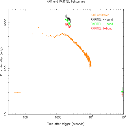
Figure 4: PAIRITEL and KAIT light curves for GRB 080310. The KAIT unfiltered data are calibrated to the $R$-band. All data have been corrected for dust extinction.

2.11 Gemini

Our last optical data were acquired with Gemini-North using the Gemini Multi-Object Spectrograph (GMOS) in imaging mode with the $r$-band filter. The observations began at 10:22UT on 19th March 2008 and consisted of $5\times 150$ second exposures. The data were reduced using the gemini-gmos routines within iraf. No significant flux was detected at the location of the afterglow, as reported in Table A5.

2.12 Polarization

Three linear polarimetric observation sets were carried out with the ESO-VLT during the late afterglow evolution as shown in Table 1. The observations allowed us to derive rather stringent upper limits although still compatible with past late-time afterglow detections (Covino et al. 2005, see also, however, Bersier et al. 2003) and substantially lower than the early time afterglow measurement by Steele et al. (2009) for GRB 090102. In the case of GRB 090102, however, the detection is taken at 160 seconds; a time when Steele et al. (2009) argue that the flux should be dominated by reverse shock emission.

The detection of linear polarization at the level of a few percent in the light from GRB optical afterglow is well within the prediction of the external shock scenario (Zhang & Mészáros 2004, and references therein) and indeed it is still one of the most relevant observational findings supporting it (e.g., Covino 2010). On the other hand, a comprehensive framework predicting the polarization degree and position angle evolution during the afterglow had to deal with the increasing complexity and variety of behaviours shown by the afterglow population. In general, the late-afterglow optical polarization is related to three main ingredients: the emission process able to generate highly polarized photons (i.e., synchrotron), the ultra-relativistic motion and the physical beaming of the outflow (Ghisellini & Lazzati, 1999; Sari, 1999). Therefore the polarization time-evolution is in principle a powerful diagnostic of the afterglow physics, and many attempts were carried out to compare observations to models (e.g., Lazzati et al. 2003, 2004) with particular emphasis to the jet structure (Rossi et al., 2004).

During the polarimetric observations of GRB 080310 the afterglow showed a smooth decay (see Figure 3) without any detectable temporal break or spectral change. Polarization below $\sim 2.5$% cannot put specific constraints on the afterglow modeling or the jet structure. These results, are however compatible with what would be expected at late times, as this is when the forward shock should dominate emission and the magnetization signal of the fireball is lost in the interaction with the surrounding medium.

Table 1: ESO-VLT polarimetric observations of the late afterglow of GRB 080310

$t-t_{0}$ (s)	$T_{exp}$ (s)	Polarization (%)	Band
87171	1447	$<2.5$	$V$
169501	1447	$<2.5$	$V$
253724	4607	$<2.6$	$V$

2.13 Observations from literature

Data from the Palomar 60 inch telescope (Cenko et al., 2006) were obtained from the Palomar 60 inch-Swift Early Optical Afterglow Catalog (Cenko et al., 2009), in which the 29 GRBs between the 1${}^{\textrm{st}}$ of April 2005 and the 31${}^{\textrm{st}}$ of March 2008 with P60 observations beginning within the first hour after the initial Swift-BAT trigger are presented.Cenko et al. (2009) reduce data in the iraf environment, using a custom pipeline detailed in Cenko et al. (2006). Magnitudes were calculated using aperture photometry and calibration performed using the USNO-B1 catalog and the data were corrected for dust extinction using the extinction maps of (Schlegel et al., 1998).

Further published data for GRB 080310 were obtained from Kann et al. (2010), in which SMARTS-ANDICAM data are detailed as part of an extensive survey of optical data for GRBs in both the pre-Swift and Swift eras. Kann et al. (2010) reduce their data using standard procedures in iraf and midas. Both aperture and PSF photometry were used in the derivation of magnitudes, when comparing to standard calibrator stars.

The 0.6m Super-LOTIS (Livermore Optical Transient Imaging System) telescope, located at the Steward Observatory (Kitt Peak, Arizona; Pérez-Ramírez et al. 2004) began $R$-band observations of the error region of GRB 080310 at 08:38:43 UT, 44 seconds after the start of the burst (Milne & Williams, 2008). The OT detected by Chornock et al. (2008) and confirmed by Cummings et al. (2008) was not apparent in the initial images, even when stacking the first three 10 second exposures. However, the subsequent 20 second exposures do show the optical transient without stacking, which suggests that the GRB brightened in the $R$-band during the first two minutes after detection. A nearby USNO-B star was used to derive the $R$ magnitude.

3 Modelling

To model the emission of GRB 080310 we begin by fitting the BAT and XRT data, before then extending the model into the lower energy bands.

3.1 Initial modelling of the high energy emission

We expand on the previous work done by Willingale et al. (2010), where a sample of 12 GRBs were selected and fitted using the pulse model of Genet & Granot (2009). In this model, the prompt emission component of GRB emission is split into a series of pulses, where each pulse is considered to be the result of a relativistically expanding thin spherical shell that emits isotropically. It was assumed that each of the pulses was in the fast cooling regime (Sari et al., 1998) and that each of the X-ray and $\gamma$-ray spectra could be fitted with a temporally evolving Band function (Band et al., 1993). A Band spectral energy distribution is a smoothly broken power-law. Below, we show a modified Band function, which includes temporal evolution.

$$B(z)=B\left\{\begin{array}[]{ll}z^{b_{1}-1}e^{-z},&\mbox{$z$ $\leq$ $b_{1}-b_{2}$,}\\ z^{b_{2}-1}\left(b_{1}-b_{2}\right)^{b_{1}-b_{2}}e^{-\left(b_{1}-b_{2}\right)},&\mbox{$z$ $>$ $b_{1}-b_{2}$,}\\ \end{array}\right.$$ (1)

where

$$z=\left(\frac{E}{E_{f}}\right)\left(\frac{T-T_{ej}}{T_{f}}\right)^{d}.$$ (2)

The times in Eqn 2 are all in the observed frame, where $T_{ej}$ is the time of shell ejection from the central engine and $T_{f}$ is the time at which the last photon arrives from the shell along the line of sight. $B$ is the normalisation to the Band function, with $b_{1}$ and $b_{2}$ being the low and high energy photon indices of the Band function, respectively. The spectral shape of each pulse evolves in time as determined by the temporal index $d$. In Willingale et al. (2010) $d=$ -1 due to the assumption that the emission process is synchrotron under the standard internal shock model. It is this value of temporal index that was also used by Genet & Granot (2009) in the original derivation of the pulse profiles, meaning that only a value of $d=$ -1 is strictly consistent with the original pulse model.

The prompt pulse model describes the morphology of the prompt light curve and the rapid decay phase as observed in the high-energy bands. In addition to this, an afterglow component was also included in the modelling as outlined in Willingale et al. (2007). The afterglow component has a functional form as outlined in Eqn 3, which comprises an exponential phase that transitions into a power-law decay.

$$f_{a}\left(t\right)=\left\{\begin{array}[]{ll}F_{a}\exp\left(\alpha_{a}-\frac{t\alpha_{a}}{T_{a}}\right)\exp\left(\frac{-T_{r}}{t}\right),&\mbox{$t$ $<$ $T_{a}$,}\\ F_{a}\left(\frac{t}{T_{a}}\right)^{-\alpha_{a}}\exp\left(\frac{-T_{r}}{t}\right),&\mbox{$t$ $\geq$ $T_{a}$.}\\ \end{array}\right.$$ (3)

In Eqn 3, $f_{a}\left(t\right)$ is the flux from the afterglow at time $t$, $F_{a}$ gives the flux at the transition time between the exponential and the power-law components, $T_{a}$. $T_{r}$ is the rise time and finally $\alpha_{a}$ is the index that governs the temporal decay of the power-law phase.

Combining the prompt pulses and the afterglow component we adopted the same method of fitting the data from the Swift BAT and XRT instruments as Willingale et al. (2010), by first identifying the individual pulses in the BAT light curve and allowing their parameters to be fitted by minimizing the $\chi^{2}$ fit statistic for both the BAT and XRT light curves. The afterglow component was then fitted by allowing the routine to find the optimum values for the characteristic times and normalizing flux shown in Eqn 3.

The simultaneous BAT and XRT fit is plotted in Figure 5 and shows several important characteristics of both the burst and the model. Firstly, there is a lot of structure evident in the light curves, particularly during the first 1000 seconds of the XRT light curves. In this fit, sixteen unique pulses have been identified and can be seen to fit the XRT data accurately. In the original fit from Willingale et al. (2010) there were only ten pulses, however this failed to fully model some of the structure in the softest BAT band (15-25 $\thinspace\rm{keV}$) between 200 and 400 seconds. The additional pulses now provide a better fit to this time, across all the BAT and XRT bands with a reduced $\chi^{2}$ statistic of 1.68 for 1212 degrees of freedom. The quality of this fit is formally not statistically acceptable, however the largest contribution to the $\chi^{2}$ value is from small scale intrinsic fluctuations in the data. The properties of the sixteen pulses are listed in Table 2.

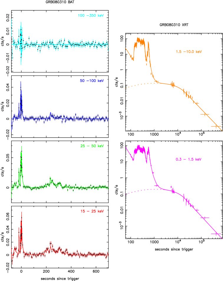
Figure 5: BAT and XRT data, showing the fitted Willingale et al. (2010) model. Left panels: BAT bands (Top to bottom: 100-350 $\thinspace\rm{keV}$, 50-100 $\thinspace\rm{keV}$, 25-50 $\thinspace\rm{keV}$ & 15-25 $\thinspace\rm{keV}$). Right panels: XRT bands (Top: XRT hard band, bottom: XRT soft band). Pulse parameters have been fixed, whilst the afterglow parameters have been fitted. Solid lines show the total fit (pulses and afterglow), whilst dashed lines show only the afterglow component to the fit.

Table 2: Properties of the prompt pulses identified in the BAT and XRT light curves. These include the peak time ($T_{pk}$), peak energy at this time ($E_{pk}$), the rise time ($T_{r}$) and arrival time of the last photon ($T_{f}$) for each pulse.

Pulse	$T_{pk}$ (s)	$E_{pk}$ (keV)	$T_{r}$ (s)	$T_{f}$ (s)	$b_{1}$
1	-52.8	200	9.7	44.5	-1.49
2	-16.0	200	5.0	6.0	-1.20
3	-4.6	200	3.8	11.7	-0.40
4	1.8	200	2.7	17.2	-1.50
5	159.0	12.3	25.3	74.0	-0.30
6	191.6	13.4	12.4	39.8	-0.02
7	210.0	21.3	10.0	46.7	-0.16
8	235.0	58.0	8.0	24.4	-0.13
9	251.8	42.0	10.0	52.4	-0.20
10	282.0	15.8	10.0	40.0	-0.10
11	308.7	16.1	15.0	32.5	0.24
12	342.7	7.8	15.0	40.1	-0.18
13	366.0	34.3	10.0	11.5	-0.38
14	390.0	1.2	23.0	56.1	0.21
15	513.8	3.8	31.1	193.8	-1.26
16	582.1	2.4	43.9	66.5	-0.09

3.2 Extrapolating to the optical and IR

Previously, no optical or IR data have been included when modelling the light curve and a fit to only the Swift BAT and XRT data has been produced (Figure 5). However, given the rapid response of optical and IR instruments to the trigger for GRB 080310 we extend the model to include these new sources of data.

The simplest approach to fitting the optical and IR light curves for GRB 080310 was to use the fitting routine from Willingale et al. (2010) and simply extrapolate the Band functions for both the pulses and also the afterglow to these lower energies. In this initial attempt all of the parameters previously discussed were held at the values obtained for the high energy fit, to see what modifications might be necessary to both components.

Figure 6: Optical and IR light curves obtained by extending the high energy fit to the prompt pulses and afterglow component.The spectral shape of the pulses is assumed to be a Band function extrapolated back to the optical and IR data ($K$, $H$, $J$, $I$, $R$, $V$, $B$ and $U$ bands). Vertical dashed lines denote times of interest later discussed, at which the SEDs are considered at in more detail. The coloured dashed lines show the afterglow component to the extrapolation for each band.

Whilst it provides an acceptable fit to the XRT and BAT bands, the original pulse model vastly over predicts the optical and IR fluxes from the pulses (Figure 6), which implies there must be a break in the pulse spectrum between the X-ray and the optical and IR energies. Such a break is expected in a synchrotron spectrum, but can also been seen in thermal spectra as the Rayleigh-Jeans tail. Additionally, the afterglow prediction from the BAT and XRT fit is not consistent with the optical data at late times where the prompt component to the light curve is negligible. Figure 6 also shows that the temporal decay index of the power-law phase of the afterglow gives rise to a decay which is more rapid than the optical data suggest.

An alternative method of reducing optical flux is to invoke dust absorption, however, as reported in Perley et al. (2008), extinction due to dust is low at $A_{V}~{}=~{}0.10~{}\pm 0.05$ at an average time of $T_{0}(+1,750)$ seconds for GRB 080310. As not only the late time emission seems unaffected by such absorption, but also by 2,000 seconds after trigger, we chose to favour a low energy spectral break in our modelling of the optical emission. The following sections of this paper detail the implementation of such alterations to the Willingale et al. (2010) model.

3.3 Modifications to the model

3.3.1 An additional spectral break

To reduce the flux from each pulse in the optical and IR light curves of GRB 080310 we introduced an additional break to the spectrum for each prompt pulse. An example of such a spectrum is shown in Figure 7, where a regular Band function has a low energy break below $E_{pk}$. To fully describe this break, three parameters are needed; a value of the break energy ($E_{a}$), the spectral index of the power-law slope in the low energy regime ($p_{a}$) and a temporal index which describes how the break energy evolves in time ($d_{a}$). The value of $E_{a}$ is defined at $T_{pk}$, when the emission from the pulse is at a maximum. The entire pulse spectrum already evolves in time, according to the index $d$ as shown in Eqn 2, and so the expectation was that the time evolution of $E_{a}$ would be related. Previously a value of $d=$ -1 was used, which when integrating of the Equal Arrival Time Surface (EATS) means a pure Band function can be recovered in the source frame given a Band function in the observed frame. Other values of $d$ prevent assumptions to be made concerning the source spectrum. We allowed the index $d_{a}$ to be fitted independently, to test whether the evolution of the break was the same as the rest of the spectrum. Again, we note that only $d_{a}=$ -1 is fully consistent with the original Genet & Granot (2009) pulse model. The functional form of the new spectral model for each pulse is shown in Eqn 4.

Figure 7: Example modified spectrum including additional spectral break.

$$N(E)=\left\{\begin{array}[]{ll}AE^{p_{a}-1}\exp\left(\frac{-E_{a}}{E_{c}}\right)E_{a}^{-\alpha},&\mbox{ $E$ $\leq$ $E_{a}$,}\\ AE^{b_{1}-1}\exp\left(\frac{-E}{E_{c}}\right),&\mbox{ $E_{a}$ $<$ $E$ $\leq$ $E_{pk}$,}\\ AE^{b_{2}-1}\exp\left(\alpha-\beta\right)E_{pk}^{-(\alpha-\beta)},&\mbox{ $E$ $>$ $E_{pk}$.}\\ \end{array}\right.$$ (4)

The model spectrum for photon emission assumes several things. Firstly, there is a single underlying population of relativistic electrons, whose energies can be described by a broken power law such as that described in Shen & Zhang (2009). Such a spectrum of electron energies leads to a similar photon spectrum: a singly broken power-law, which corresponds to the observed Band function. However, it would be unphysical for this spectral shape to extend indefinitely to low energies, particularly as the electron energy spectrum has an associated minimum energy $E_{m}$. This minimum electron energy has a related emission energy at a frequency $\nu_{m}$. With no self-absorption, the spectral index to the emission spectrum changes to $\frac{1}{3}$ at photon frequencies below $\nu_{m}$, but if self-absorption is present then at low energies we would expect to see a steeper spectral index of 2 if the absorption frequency is less than $\nu_{m}$ or alternatively a spectral index of $\frac{5}{2}$ in the case of $\nu_{m}~{}<~{}\nu_{a}$. In the former case, if there is an intervening spectral range between $\nu_{a}$ and $\nu_{m}$, a spectral index of $\frac{1}{3}$ is expected between these two frequencies.

To keep the model simple, due to the limited nature of the spectral information available, we only included a single additional break in the spectrum. By allowing the resultant spectral index to be constrained by the observations, rather than assuming a value, we hope to better understand the physics required to explain the spectrum of prompt GRB pulses.

3.3.2 The afterglow

As seen in Figure 6, prompt pulses without a low energy break significantly over predict the observed flux in the optical and IR light curves prior to 10,000 seconds. By introducing a low energy break to the pulse spectra, we hoped to completely remove the prompt contribution to the total emission, and model the entire light curve with afterglow emission. One reason for considering this is the smooth nature of the optical light curves. Whilst there is some variation during the plateau seen between 200 and 3,000 seconds, this is at a low level, and happens smoothly over a large period of time. If the prompt pulses observed at higher energies were also the dominant source of emission at these energies, then we might expect to see similar structure in the optical and IR light curves to that shown in Figure 5.

The first issue to address with the afterglow fit was to account for the small difference in temporal decay index ($\alpha_{a}$) between the higher and lower energy bands. To do so, we included an additional parameter that described the difference in this index, and allowed it to be fitted. By including this, we could account for the slightly shallower decay of the power-law phase in the optical and IR channels. The change in $\alpha_{a}$ required was found to be small, at a value of approximately 0.2, but the associated errors in each instance showed it to be inconsistent with zero. This may be explained physically by a slight curvature in the spectrum of the afterglow between the optical and X-ray bands. This, however, is not a large enough difference to suggest a spectral break, such as the one introduced to the prompt pulses. The GRB afterglow flux is also thought to be synchrotron emission. However, at these late times the radiation is usually assumed to come from an optically thin plasma, and so a self-absorption break would be expected at energies lower than the optical bands observed for GRB 080310. We also ruled out contamination in the optical and IR wavebands as being the source of this difference as any emission from the host should be constant with time. This should add a constant offset to the data, and should the afterglow emission reach a comparable order of magnitude, a plateau at the end of the optical decay would be expected. This plateau is not observed, and the difference between the low and high energy temporal decay indices of the afterglow is also determined by data prior to when the host would be seen to make a significant impact on the optical and IR light curves.

With no prompt component capable of rising quickly, we also had to modify the manner in which the afterglow rises, to account for the rapid increase in flux seen in the V-band data at approximately 100 seconds in Figure 3. To do this, we introduced a third part to the functional form that is shown Eqn 3. This extra regime is shown in the top line of Eqn 5, and describes a power-law rise in flux, with an index of 2. We also allowed the afterglow to be launched at a time that was independent to the trigger time of the GRB, by introducing a launch time ($T_{l}$), which offsets the afterglow in time to better fit the timing of the rise observed in the V-band. These modifications are shown in Eqn 5 and are used for the afterglow-dominated modelling only. In the case of the prompt dominated fit, we return to the afterglow model of Willingale et al. (2007) as explained in §3.5.

$$f_{a}(t)=\left\{\begin{array}[]{ll}F_{a}\exp\left(\alpha_{a}-\frac{(T_{r}-T_{l})\alpha_{a}}{T_{a}-T_{l}}\right)\left(\frac{t-T_{l}}{T_{r}-T_{l}}\right)^{2},&\mbox{ $t$ $\leq$ $T_{r}$,}\\ F_{a}\exp\left(\alpha_{a}-\frac{(t-T_{l})\alpha_{a}}{T_{a}-T_{l}}\right),&\mbox{ $T_{r}$ $<$ $t$ $\leq$ $T_{a}$,}\\ F_{a}\left(\frac{t-T_{l}}{T_{a}-T_{l}}\right)^{-\alpha_{a}},&\mbox{ $t$ $>$ $T_{a}$.}\\ \end{array}\right.$$ (5)

3.4 Afterglow dominated fit

Given the smooth nature of the optical and IR light curves, our initial use of the low-energy spectral break in the prompt pulse spectrum was to remove the prompt component to the optical light curves entirely, and try and explain the early time behaviour with only afterglow emission. To do this, the prompt pulses were initially switched off from the optical and near infrared fit. With these removed, the afterglow parameters $T_{l}$, $T_{r}$, $T_{a}$, $F_{a}$, $\alpha_{a}$ and the change between optical and high energy values of $\alpha_{a}$ were fitted. Having obtained values for these parameters using the fitting routine, we re-introduced the prompt pulses, allowing $p_{a}$ to be fitted, to find the minimum break in the pulse spectra required to remove the prompt optical and IR flux. Where the fit statistic tended to unphysical values of $p_{a}$ we checked the effects of forcing $p_{a}$ to be $\frac{5}{2}$. When this was undertaken, we found that whilst there was an increase in the reduced $\chi^{2}$ statistic, this was incredibly small, approximately $1\times 10^{-3}$,for 1642 degrees of freedom.

3.4.1 Light Curves

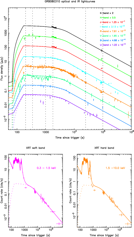
Figure 8: Simultaneous fit to optical, IR and XRT data, in which the early time optical and IR are fitted by the afterglow emission. Top panel: Optical and IR bands fitted with low energy break ($K$, $H$, $J$, $I$, $R$, $V$, $B$ and $U$ bands). Bottom left: XRT soft band fit. Bottom right: XRT hard band fit. The afterglow parameters are fitted, as are values for $d_{a}$, whilst $E_{a}=$ 0.3 keV and $p_{a}$ has been set to $\frac{5}{2}$. Coloured dashed lines show the afterglow component in each band. The reduced $\chi^{2}$ for this fit is 2.44 with 1,642 degrees of freedom.

Figure 8 shows the light curves for the best fit found using the method described above, for which a reduced $\chi^{2}$ value of 2.44 with 1,642 degrees of freedom was found. The late time XRT afterglow isn’t as well fitted as in the original Willingale et al. (2010) method (Figure 5), where only the high energy bands were included. This is particularly the case for the last data points, and those at the transition between the prompt and the afterglow phase in the X-ray bands. The cause of this is due to the greater number of optical points being the largest constraint on the afterglow parameters, particularly the characteristic times, $T_{a}$ and $T_{r}$. Because these times have changed from the original fit, the temporal decay index in the power-law phases has reduced from $1.58^{+0.04}_{-0.03}$ to $1.30^{+0.01}_{-0.01}$. The afterglow parameters all have a reduced error in this newer fit as the optical and IR data points allow for more accurate fitting with a greater quantity of data. The characteristic times also have improved accuracy, with $T_{r}$ = $223^{+16}_{-20}$ seconds, $T_{a}$ = $6,368^{+495}_{-50}$ seconds and $T_{l}$ = $120^{+9}_{-11}$ seconds. The errors quoted in this instance were obtained when floating all of the parameters mentioned simultaneously. Once the afterglow parameters were in place, the final bulk value of $p_{a}$ was found to tend to $5.6$, with a 1$\sigma$ lower limit of 5.5 and an unconstrained upper limit. The lower limit is tightly constraining, and likely due to the fitting routine trying to remove contributions from the brightest early pulses, which therefore affects the value assigned to the weaker pulses as well. The lack of an upper limit suggests that the fitting routine is attempting to remove the prompt component entirely from the optical emission, as driven by the morphology of the light curve particularly the dense sample of KAIT data points. The value of 5.6 is very significantly steeper than that expected at either 2 or $\frac{5}{2}$. The suggested lower limit from the $\chi^{2}$ distribution is surprisingly tight, given the shape of the curve obtained for the statistic when only varying $p_{a}$ as the distribution is remarkably flat for a broad range of values. Looking at the fit statistic by eye, it would appear that the expected values from synchrotron or thermal spectra are not entirely ruled out, but lie within the lower limits of where the fit is a faithful representation of the data. To test this, we forced $p_{a}$ to a value of $\frac{5}{2}$ for all the prompt pulses, and noticed that the value for the $\chi^{2}$ statistic increased by a nearly negligible amount. By using $p_{a}$ = $\frac{5}{2}$ self-absorption becomes a viable explanation for the physical mechanism causing the observed level of optical and near infrared flux. It is therefore this value that was adopted for $p_{a}$ for the prompt pulses when trying to suppress them at early times in the lower energy regimes.

The broad scale morphology of the optical and NIR light curves are described by the fast rising afterglow, with the rise observed in the $V$-band being fitted and the level of flux of the plateau seen between 100 and 1,000 seconds being consistently modelled in five of the six bands in which it can be seen. The exception to this is that the $U$-band model light curve morphology seems to over-predict the emission actually observed in the first 1,000 seconds, which may be a result of the correction required to removed the effects of absorption from the Lyman forest as described in the section detailing the UVOT observations. The $I$-, $R$- and $V$-band data during this plateau phase do appear to have a slight dip in flux, which is not picked up by the afterglow fit. Additionally, the first $V$-band points indicate a decline in flux prior to the launching of the afterglow. To fit this, one of the early time pulses would have to be switched on at low energies, implying that at the earliest times the prompt component is still important in the optical and IR regimes.

The $V$-band data between 100 and 1,000 seconds are from three sources, VLT $V$-band, UVOT $v$-band and the UVOT white filter, which is normalised to the $v$-band. This normalisation is done at a time when there is near simultaneous UVOT $v$-band and white filter coverage. The white data are then adjusted at this time, to make the observed flux the same as that in the $v$-band. The same correction factor is then applied to all the white filter points, which relies on an intrinsic assumption that the spectrum is not varying between the $v$-band and white filter for all observations. If the total GRB low energy emission is primarily from the afterglow, this assumption is accurate, as the spectral break in the Band function will not migrate to the optical part of the spectrum. We noted, upon inspection of the data, that the UVOT points between 300 and 2,000 seconds appear to not be entirely consistent with the near simultaneous VLT data. The VLT flux values have much lower associated error, which led to us reprocess the UVOT data, to verify the values. Doing this we obtained the same UVOT fluxes. To account for the discrepancy, we introduced a systematic error in the UVOT points at the level of 10% of the measured flux for each datapoint. Analysis of only the VLT data, still shows the deficit of flux, which we discuss throughout this work, at a level that is significant given the small errors associated with the data. As this feature is significant in instruments other than UVOT, we believe that the discrepancy from the UVOT instrument does not impinge on the main conclusions of this work.

Figure 3 would suggest that the decline in flux is not marked by a change of instrument.

The temporal index $d_{a}$ governing the time evolution of $E_{a}$ is tightly constrained in this model, to a value of $d_{a}$ = $-1.01^{+0.05}_{-0.03}$. Not only does this match the temporal evolution of the characteristic energy $E_{c}$ in Genet & Granot (2009), but the 1-$\sigma$ errors quoted are restricting. Having analysed the one dimensional $\chi^{2}$ surface, it is clear that a more rapid evolution of the temporal index allows the prompt pulses to peak at earlier times, when the normalising flux at the peak of each pulse is still significant, causing an over-prediction of early time flux. At lower values the $\chi^{2}$ distribution is fairly flat, as the prompt flux normalisation is so low, it cannot be seen to contribute to the total light curve.

3.4.2 Spectral Energy Distributions

Another way of comparing the model to the observed data is to consider the spectral energy distribution (SED) at fiducial times. The times selected are indicated in Figures 6, 8 and 10 as dashed vertical lines. These correspond to times of 350 seconds (where there are early-time optical data and the activity in both the X-ray and $\gamma$-ray bands), 1,800 seconds (a time where the high energy only model shown in Figure 6 suggests the afterglow is becoming significant), $2.5$ $\times$ $10^{4}$ and $1$ $\times$ $10^{5}$ seconds (both of which are later times that should be dominated by the afterglow). Figure 9 shows the model SED at these times, and also those at both 200 and 1,000 seconds. The times shown were chosen to both allow for comparison with the maximum number of bands (both optical and X-ray) at each time and to show times where the SED can discriminate between prompt and afterglow emission at optical and IR energies.The SEDs shown in Figure 9 are those for the fit where the afterglow dominates the entire low energy emission. In each case, error bars are plotted, but in some panels are too small to be seen.

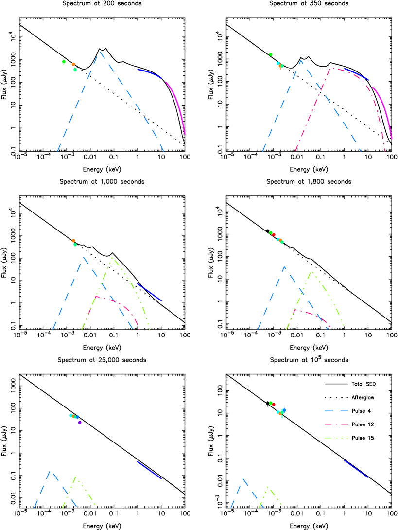
Figure 9: SEDs for fiducial times in the light curve of GRB 080310 using the afterglow model to fit the early time, low energy emission. Prompt pulses are included with a bulk value of $p_{a}$ = 2.5. The solid line is the total SED and the dotted line is the contribution from the afterglow component. Pulses 4, 12 and 15 are also shown by the dashed and dotted lines as outlined in the key shown in the bottom right panel. These are included as examples to show the evolution of some of the longer lasting pulses in the fit. The colours of the data points follow the same scheme as that used in the light curves, with the BAT and XRT data being represented by lines which extend along their entire coverage.

Figure 9 shows that by combining the prompt pulses and the afterglow component, the model SEDs have complicated structure at high energies. The first panel shows the SED at 200 seconds, a time by which the first six pulses have peaked. As an example of time evolution, the spectral contribution from pulse four is shown with the dashed line in this and subsequent panels. The temporal evolution of pulses 4, 12 and 15 can be traced through all six panels. At 200 seconds pulse 4 is the one of the three pulses causing deviation from the afterglow Band function (the others being pulses 1 and 6). Following it through all six panels of Figure 9 shows the general evolution of all the pulses. The peak flux reduces with time, and the energy at which this peak is seen becomes lower with increasing time also. By the late panels, the component of pulse 4 can still be seen on the axes, however, being several orders of magnitude lower than the afterglow Band function, it does not produce an observable feature in the total SED. Because the spectral index for all the pulses is at a value of $p_{a}$ = 2.5, before the peaks migrate to the optical regime, their contribution to the total flux at these energies is negligible. Once the peak has had time to evolve to such energies, the normalizing flux has been diminished, so the pulse contributions remain negligible.

Figure 9 also shows that the dominant pulses in the SED of GRB 080310 do not have to be those most recently launched. Pulse 12 is emitted after pulse 4, as shown in the first two panels of the figure. Despite this, pulse 12 has disappeared entirely by $2.5$ $\times$ $10^{4}$ seconds, whilst the earlier pulse can still be seen on the axes, even though the modelled emission is at a level significantly below the total SED. The bottom two panels show late times in the light curve, where only the afterglow contributes flux to the total SED. Looking only at the afterglow in all six panels, it can be seen that it varies very little at early times. This is due to the combination of a quick rise time after an early launch with a late transition time between the exponential and power-law decay phase for the afterglow component. This implies that there is a period where the afterglow effectively plateaus for a few thousand seconds. This behaviour can be identified in the light curves shown in Figure 8.

The SEDs in Figure 9 suggest that the optical emission is fitted by the extrapolation of the afterglow Band function, particularly at late times. The second panel is perhaps the most puzzling as the optical and near infrared data are aligned approximately with the afterglow SED, however there is a clear dip in the light curves, which suggests that a component which simply rises then falls smoothly cannot explain the morphology that is seen. We have not tried to fit a low energy break to the afterglow Band function, as discussed previously, because such a break is expected at energies well below the $H$-band, due to the optically thin nature of the circumburst medium. Additionally, the correct level of flux has been reproduced without the introduction of a further spectral break.

3.5 Early time prompt dominated fit

By fitting the optical and IR emission with only a significant afterglow component, there were discrepancies between the model and the data. Namely the potential decay before the sharp rise observed in the $V$-band and the deficit in flux observed in the $I$-, $V$- and $R$-bands between 300 and 2,000 seconds. In addition to this, the $U$-band data are over predicted, which is possibly due to the absorption correction from the Lyman forest as previously discussed, or alternatively could be better described with an alternative model. In an attempt to explain these features, we considered a model where these early-times were dominated by the prompt emission in the optical and near infrared regimes.

3.5.1 Light Curves

We first only considered the prompt pulses, by turning off the afterglow component and fitting only prior to 2,000 seconds. Once the early time emission was fitted, we then included the afterglow to account for the late time emission. The potential for degeneracy between $p_{a}$ and $E_{a}$ was considered, as the energy difference between the X-ray data and the optical and IR bands is over two orders of magnitude, while the $U$- and $K$-bands are only separated by less than a single order of magnitude. Data were not taken simultaneously in these two bands which are the most spectrally separated. It is therefore difficult to determine both $E_{a}$ and $p_{a}$ independently. For this reason the break energy was set to a value of 0.3 $\thinspace\rm{keV}$ (at $T_{pk}$) which is the soft end of the XRT spectral range. This implies that the fit to the high-energy regime remains unaltered, whilst giving the maximum energy range in the SED between $E_{a}$ and the optical and IR bands. Therefore the value for $p_{a}$ obtained is a lower limit, as moving $E_{a}$ to lower values would steepen the power-law index in the low energy part of the spectrum.

Initial attempts to model the low energy flux with prompt pulses held the parameters $p_{a}$, $d_{a}$ and $E_{a}$ to the same value for all pulses. This led to a bulk value of $p_{a}$ = $0.65_{-0.02}^{+0.02}$, which is significantly different from the spectral index of the Band function below $E_{pk}$, but not consistent with the expected values of $p_{a}$ if self-absorption was having an effect on the emission that is observed. The 1$\sigma$ limits on this value do not include $\frac{1}{3}$, which is what would be expected if there is an absence of self-absorption, and the optical and IR bands are below the emission frequency of electrons with the minimum energy in the electron population. The reduced $\chi^{2}$ value is 3.61 in this instance, with 1,642 degrees of freedom. There were still some issues with this fit, such as the fit not describing the slight decay followed by sharp rise in flux seen in the $V$-band. So we decided to allow all pulses to have independent values of $p_{a}$, to see if this could account for the features seen in the data. The method adopted to do this remained the same as that for the bulk value of $p_{a}$, and the light curves obtained are shown in Figure 10.

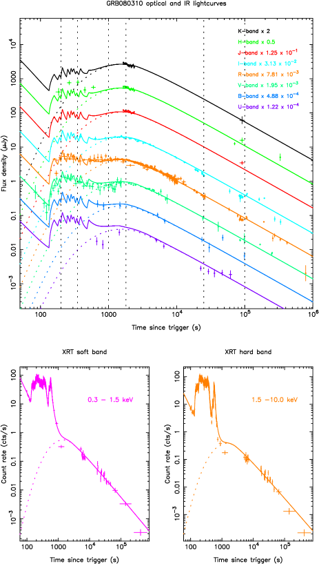
Figure 10: Simultaneous fit to optical, IR and XRT data, in which the early time optical and IR are fitted by the prompt emission. Top panel: Optical and IR bands fitted with low energy break ($K$, $H$, $J$, $I$, $R$, $V$, $B$ and $U$ bands). Bottom left: XRT soft band fit. Bottom right: XRT hard band fit. $E_{a}=$ 0.3 keV, $p_{a}$ and $d_{a}$ are allowed to float (producing a value of $d_{a}=$ -1.01) and the afterglow parameters ($T_{r}$, $T_{a}$, $\alpha_{a}$ and $F_{a}$) are also fitted. The reduced $\chi^{2}$ for this fit is 2.43 with 1,642 degrees of freedom.

Given the choice of two afterglow models; the original functional form of Willingale et al. (2007) and the modified version shown in Eqn 5, we found that in this instance, the better fit was obtained with the former, as the smoother peak to the afterglow component allowed for a closer fit to some of the $J$-, $K$- and $H$-band data at this time. This also removed a free parameter from the fitting routine. We still retained the difference between optical and high energy $\alpha_{a}$ to describe the late time decay. With these modifications, the early time prompt dominated model had a reduced $\chi^{2}$ of 2.43 for 1,642 degrees of freedom. This is significantly better than the prompt model with a bulk value of $p_{a}$ for all pulses, with a change in total $\chi^{2}$ of over 1,850.

There are little data to constrain $p_{a}$ for the first four pulses, which are predominantly observed with BAT, and so these values have large associated uncertainties. Despite this, it was clear that a large value of $p_{a}$ was required for pulses 1, 2 and 4, to allow for the decay and subsequent rise seen in the $V$-band data. The best fit to the initial decay was found by modelling it with pulse two, and suppressing pulses one and three so that they did not contribute to the optical and IR emission observed from the beginning of the optical coverage. When actually fitted, the values of $p_{a}$ for pulses 1, 2 and 4 all were larger than $\frac{5}{2}$, and so in the same manner as all the prompt pulses in the afterglow-dominated model, these were set to $p_{a}$ = $\frac{5}{2}$ as Figure 10 shows that the sharp rise is now well fitted by the rise of pulse four in a similar way to the simultaneous rise seen in the XRT data. The data obtained from KAIT have an earlier point at 57 seconds, which does not show this decay, it is difficult to fit this individual point, as whilst it is at an ideal time to investigate the prompt optical behaviour of the GRB, it is a 30 second observation, and so it is an average over a time during which large variations might be expected. This is why we have not tried to fully explain this point with our model and have removed it from the fitting undertaken. Indeed, non-detections from both Super-LOTIS and RAPTOR (Wozniak et al., 2008) at similar times to this KAIT datapoint offer further evidence towards the faintness of the emission in the optical regime at this time.

Analysis of the residuals for the optical, IR, XRT and BAT data show there are three clear contributions to the total $\chi^{2}$ statistic. The first contribution to the fit statistic is from the XRT afterglow component of the model. This deviates from the observed data at two times. Firstly, the transition from the rapid decay phase to the afterglow shows an over prediction by the model, as do the data after $10^{5}$ seconds. The latter of the two features could be explained by a late temporal break in the X-ray afterglow. Such a break should be achromatic, and therefore also observed in the late-time optical data. The final $R$-band observation, at approximately nine days after the trigger, is fainter than the extrapolation from the final power-law decay in the afterglow-dominated model, which would support the possibility of a jet break. With the prompt-dominated optical and IR model, there is a suggestion of either a plateau or rebrightening at approximately one day after the trigger, followed by a steeper decay. In both models, the data are too sparse to justify the inclusion of further parameters in the late-time modelling of the optical data.

The next significant contribution to the value of $\chi^{2}$ comes from the early-time REM data points between 150 and 600 seconds in the $H$-band. These are under predicted by the model as shown in Figure 10. Due to the sparse nature of the NIR data at this time, the fit is driven by the more densely sampled $V$- and $R$-band data. This discrepancy is better highlighted in the SEDs shown in Figure 11.

The other notable source of contribution to the fit statistic is the KAIT data. The data were initially reported in unfiltered magnitudes, with values ranging between 17^m and 20^m, and errors typically less than a tenth of a magnitude. With such small errors for over two hundred data points the contribution to the total validity of the fit from the intrinsic scatter of the dataset is significant, despite the fact that the data and model can be seen to agree by eye.

3.5.2 Spectral energy distributions

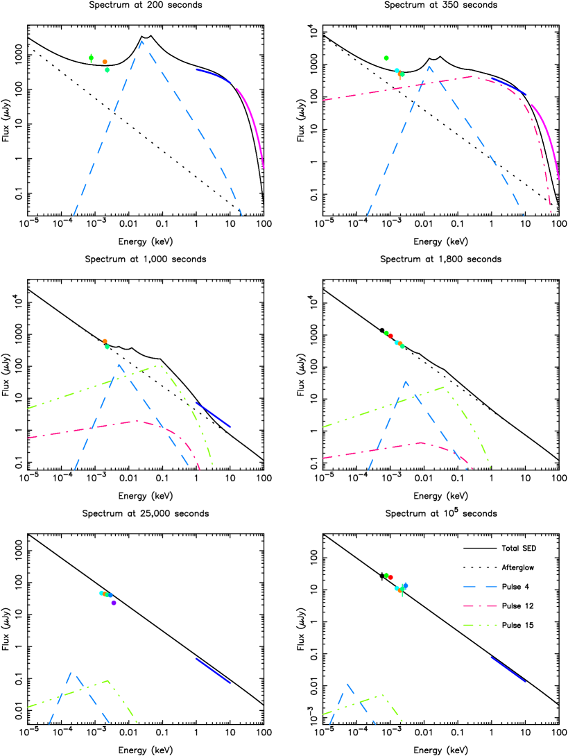
Figure 11: SEDs for fiducial times in the light curve of GRB 080310 using the prompt-dominated early time model. The solid line is the total SED and the dotted line is the contribution from the afterglow component. Pulses 4, 12 and 15 are also shown by the dashed and dotted lines as outlined in the key shown in the bottom right panel. These are included as examples to show the evolution of some of the longer lasting pulses in the fit. The colours of the data points follow the same scheme as that used in the light curves, with the BAT and XRT data being represented by lines which extend along their entire coverage.

As can be seen in the SEDs shown in Fig. 11, by introducing the prompt component to the spectrum of GRB 080310, each SED has structure beyond the simple Band function of the afterglow at earlier times in the low energy bands. For the prompt-dominated model of the early-time low energy emission, the spectral indices typically lie in the range -0.65 $<$ $p_{a}$ $<$ 1. This does not include the earliest pulses, which have a necessarily steep spectral index to prevent their emission dominating (and poorly fitting) the optical and IR light curves. These have been fixed to a value of $p_{a}$ = $\frac{5}{2}$, as well as pulses 8 and 16, which also require steep indices.

Unlike in the afterglow-dominated model, the SED at 350 seconds shows the optical and IR (particularly the $H$-band) model to disagree with the data; this is the most valuable of the SEDs in Figure 11, as it is one of the only two prior to the afterglow making the dominant contribution to the total low energy emission, and of these two has the best low energy coverage. The $R$-, $I$- and $V$-band data at this time are at approximately the correct level of flux for each band, although the $I$-band and $R$-band deviate from the expected shape of the SED. However the $H$-band data (which offers the largest range of spectral information when considered with the other three bands) is noticeably under predicted, as corroborated by the light curves in Figure 10. When inspected by eye, the four bands at this time could be thought to lie on a single power-law with a spectral index similar to that of the afterglow. This would lend more credence to the afterglow -dominated early-time optical and near infrared model.

The subsequent SEDs are all dominated by the Band function of the afterglow at optical and IR energies, and, despite the use of the original Willingale et al. (2007) afterglow model and changes in $T_{a}$, $F_{a}$, and $T_{r}$, the late time fit is similar to that obtained for the afterglow -dominated fit. The optical and near infrared data points are all over predicted at $2.5$ $\times$ $10^{5}$ seconds, which something that can be seen by looking at the light curves, particularly in the case of the UVOT $u$-band data. The $u$-band dataset displays some unusual characteristics, being significantly fainter than expected prior to 1,000 seconds and then appearing to plateau between $2$ $\times$ $10^{4}$ and $1$ $\times$ $10^{5}$ seconds. We considered the removal of this dataset from the analysis, but as both the values of parameters obtained for the best fit seem largely insensitive to the $u$-band data we retained them. This is a result of the relatively sparse coverage in the $u$-band, principally in comparison to that of the $R$-band, the weighting of the $u$-band data in determining the fit statistic is small.

4 Discussion

For direct comparison between the two models discussed in the previous section, their parameters have been included in Table 3. Given the degeneracy between $E_{a}$ and $p_{a}$ it isn’t possible to simultaneously fit exact values to both without a more extensive low energy coverage over a larger range of wavelengths. Because of this, $E_{a}$ was fixed at 0.3 keV, in an attempt to find a value of $p_{a}$.

Table 3: Pulse $p_{a}$ values and afterglow parameters for both the prompt and afterglow dominated early time optical emission models. Note that the value for $T_{l}$ in the prompt dominated model is untabulated, as the Willingale et al. (2007) model was used for the afterglow in this instance. All instances where $p_{a}$ = $\frac{5}{2}$ have the values fixed rather than fitted, and so no uncertainties were calculated for them.

Parameter	Parameter description	Afterglow	Prompt
		dominated	dominated
$p_{a}$ (pulse 1)	X-ray to optical spectral index	2.5	2.5
$p_{a}$ (pulse 2)	X-ray to optical spectral index	2.5	2.5
$p_{a}$ (pulse 3)	X-ray to optical spectral index	2.5	-0.65${}^{+0.59}_{-0.59}$
$p_{a}$ (pulse 4)	X-ray to optical spectral index	2.5	2.5
$p_{a}$ (pulse 5)	X-ray to optical spectral index	2.5	0.03${}^{+0.04}_{-0.07}$
$p_{a}$ (pulse 6)	X-ray to optical spectral index	2.5	0.11${}^{+0.46}_{-0.17}$
$p_{a}$ (pulse 7)	X-ray to optical spectral index	2.5	-0.11${}^{+0.43}_{-0.25}$
$p_{a}$ (pulse 8)	X-ray to optical spectral index	2.5	2.5
$p_{a}$ (pulse 9)	X-ray to optical spectral index	2.5	-0.06${}^{+0.09}_{-0.01}$
$p_{a}$ (pulse 10)	X-ray to optical spectral index	2.5	-0.01${}^{+0.26}_{-0.26}$
$p_{a}$ (pulse 11)	X-ray to optical spectral index	2.5	-0.11${}^{+1.00}_{-0.30}$
$p_{a}$ (pulse 12)	X-ray to optical spectral index	2.5	0.17${}^{+0.19}_{-0.11}$
$p_{a}$ (pulse 13)	X-ray to optical spectral index	2.5	1.0${}^{+0.22}_{-0.22}$
$p_{a}$ (pulse 14)	X-ray to optical spectral index	2.5	0.04${}^{+0.11}_{-0.08}$
$p_{a}$ (pulse 15)	X-ray to optical spectral index	2.5	0.35${}^{+0.08}_{-0.09}$
$p_{a}$ (pulse 16)	X-ray to optical spectral index	2.5	2.5${}^{+}_{-}$
$T_{l}$ (seconds)	Afterglow launch time	120${}^{+9}_{-11}$	-
$T_{r}$ (seconds)	Afterglow rise time	223${}^{+16}_{-20}$	1000${}^{+435}_{-131}$
$T_{a}$ (seconds)	End time of afterglow plateau phase	6368${}^{+501}_{-495}$	2937${}^{+1056}_{-1346}$
$\alpha_{a}$	Afterglow temporal decay index	1.30${}^{+0.01}_{-0.01}$	1.31${}^{+0.01}_{-0.01}$
$\Delta\alpha_{a}$	$\Delta\alpha_{a}$ between optical and X-ray decays	0.21${}^{+0.03}_{-0.04}$	0.18${}^{+0.1}_{-0.03}$
$F_{a}$ ($\gamma$.cm-2.s-1)	Integrated Flux at $T_{a}$	2.34${}^{+0.08}_{-0.08}$ $\times$ 10-2	2.77${}^{+0.23}_{-0.16}$ $\times$ 10-2

There is no clear difference in the fit statistic for either of the models presented in this work. The difference in total $\chi^{2}$ is less than 30 over such a large range of degrees of freedom. Whilst numerically, this difference is in favour of the prompt-dominated early-time optical and near infrared model, we do not believe that the magnitude of the difference is enough to warrant favouring one model above the other.

For the afterglow-dominated early-time model the fitted bulk low-energy spectral index for the prompt pulses is unphysically steep ($p_{a}$ = 5.6). However, the change in fit statistic when forcing this value to one consistent with self-absorption was near negligible, which is why we therefore adopted the less extreme value. In contrast, most values of $p_{a}$ are more reasonable (-0.65 $<$ $p_{a}$ $<$ 1) when the early-time low-energy emission is dominated by the prompt pulses identified at higher energies. This is not, however, true for all the pulses. It was necessary to suppress pulses 1, 2, 4, 8 and 16 with positive, steep low energy spectral indices so that the optical and IR emission was not over predicted. To understand this behaviour we looked at the one dimensional $\chi^{2}$ distribution for $p_{a}$ of the earliest of these three pulses. We found that the distribution reduced asymptotically at higher values of $p_{a}$, meaning that there was no clear minimum. However, the actual reduction in the fit statistic achieved by reducing the low energy spectral index rapidly dropped, so this decrease in $\chi^{2}$ value quickly stopped making a significant difference to the quality of the total fit compared to other contributions to the $\chi^{2}$ statistic. After establishing this, we again adopted values of $p_{a}$ = $\frac{5}{2}$ in these instances, with a minimal increase of $\chi^{2}$ being introduced as a result.

Given the variations in $p_{a}$ for the prompt dominated model, we tried to relate these values to other parameters of the pulses, such as pulse duration ($T_{pk}$) and the low energy photon index of the Band functions for each pulse ($b_{1}$). We found no correlations between $p_{a}$ and the other pulse parameters.

In the afterglow dominated fit, the prompt component is several orders of magnitude fainter than the observed emission. Additionally, with positive values of $p_{a}$, time is required for the peak of the pulse spectrum to migrate to the optical and IR bands, before which the spectrum is rising at these energies. The pulse emission is largest around $E_{a}$, the evolution of which is governed by the temporal index $d_{a}$, which has been shown to be negative. This means that the pulse energy decreases with increasing time. In addition to this, the normalization of each pulse scales with $t^{-1}$, which means that when the peak of emission reaches the optical part of the spectrum the total flux is reduced. To illustrate the prompt component in this scenario, we subtracted the afterglow component from the afterglow-dominated model, and produced Figure 12, which shows the $H$-band prompt-only light curve that underlies the afterglow emission.

Figure 12: Modelled $H$-band light curve showing the prompt component only for the afterglow dominated fit.

The afterglow-dominated, early-time optical model required three alterations to the afterglow component; a change of temporal power-law index between high and low energies, a power-law rise at early times and a variable launch time $T_{l}$. However, even with these modifications, there were several features of the data that were not entirely modelled in this scenario, including the apparent decay in the $V$-band prior to the rapid rise and the slight deficit in flux between 300 and 2,000 seconds. The tendency towards unphysical values of $p_{a}$ also suggested that fitting the early-time emission with a fast rising afterglow may not provide the best model of the observed flux. The SEDs of Figure 9 confirm that the afterglow-dominated fit provides a reasonable fit to the data and that at 350 seconds, which is a time where at high energies the prompt components are dominant, the afterglow Band function fits both the level and slope of the SED.

When fitting the early-time flux with the prompt pulse emission model we first adopted a single value of $p_{a}$ which was held constant for all pulses. The low energy spectral index obtained was $p_{a}=$0.65, however most of the early time emission was hidden by the tail of one of the earliest prompt pulses. Aside from a poor fit to the $H$-band data, the fast rise seen in the $V$-band was not well represented in this instance, so the pulses were allowed to have independent values of $p_{a}$. This produced a better fit to the data, significantly improving the $\chi^{2}$ statistic. The fast rise in the $V$-band, and the small scale variations in the light curves seem to be represented well by this model. There were, however, discrepancies with this alternative. Firstly, the $H$-band data were under predicted by the model, which can be seen in both the light curves and SEDs shown for this model. The SEDs also show that, at 350 seconds, the optical SED appears to be more accurately represented by a single power-law which agrees more with the nature of the afterglow. Three of the first four pulses (and also pulses 8 and 16) tend towards an unphysically steep spectral index when fitted. As with the afterglow-dominated model, constraining the values of $p_{a}$ to $\frac{5}{2}$ in these instances does not significantly reduce the quality of the fit obtained.

The other values of $p_{a}$ for the prompt-dominated fit could be consistent with the energy bands lying below the energy of emission from the least energetic electron in the relativistic population responsible for the observed photons. We found no relation between the low energy spectral index for each pulse and any other pulse parameter, giving no insight into the cause of the variation of $p_{a}$. An interesting result is the marked difference between pulses 1, 2, 4, 8 and 16 when compared with all the other pulses. $p_{a}$ for these early pulses indicates their emission is from an optically thick environment in the optical regime. Another implication is that these pulses must be launched from a different environment than the other eleven which have far shallower spectral indices at low energies.

One additional benefit to the prompt-dominated model was the ability to return to the simpler afterglow model of Willingale et al. (2007), as the rapid rise seen in the $V$-band was attributed to the rise of pulse four.

An alteration attempted with the prompt-dominated early-time model was to introduce an offset to the onset of the afterglow. It was hoped that by allowing the afterglow to rise earlier, the SED at 350 seconds could reconciled with the model. This was found not to be possible, as this returned the model to something resembling the afterglow-dominated fit, and therefore we were unable to model the small scale variations and observed optical deficit in the plateau between 300 and 2,000 seconds.

Both of the alternative models presented in Figures 8 to 11 are poor at fitting the transition between the rapid decay phase and the afterglow plateau observed in the X-rays. We attempted to better model this by allowing the afterglow to rise at a later time than presented in either of the two fits highlighted in Table 3. By doing so, it was possible to improve the quality of the high energy afterglow fit, but to the detriment of that obtained for the optical data. With an afterglow that rises later but more quickly, the optical data between 3,000 seconds and 8,000 seconds are under predicted by the model suggested. With a larger number of data points, and correspondingly better statistics, the optical points were those that we therefore favoured. The prompt-dominated, early-time optical and IR model described in Table 3 and illustrated in Figures 10 and 11 summarize this model. Unfortunately, the XRT coverage contains a gap during the afterglow plateau phase, and therefore the exact morphology of this component, which would help significantly constrain the rise of the afterglow, is unknown at these times.

An alternative suggestion, given the acceptable fit at approximately 2,000 seconds in all the available optical IR bands, to explain the factor of two or three difference between the X-ray data and model at this time would be to include a spectral break in the afterglow spectrum. Whilst this may improve the fit at these times, the later afterglow coverage between 10⁴ and 10⁵ seconds show both the higher and lower energy bands to be modelled at the correct level.

Additionally, a large contribution to the $\chi^{2}$ distribution was from the optical and IR data, particularly the KAIT dataset, with low magnitude errors. Whilst the observational errors in these datapoints may be as reported, each of the datasets had to be calibrated so they all were in standard bands. In doing so the systematic errors associated with these data points increased. We considered this, and added a systematic of 0.03^m to every optical or IR point. The quoted values for the fit statistics include this systematic source of error.

Knowing the characteristic times of the afterglow for each of the two models allows us to calculate the initial bulk Lorentz factor in both an interstellar medium (ISM) like or wind dominated circumburst environment. To do so we used Eqns 6 (Molinari et al., 2007) and 7 (Sari & Piran, 1999).

$$\frac{\Gamma_{0,ISM}}{2}=\left(\frac{3E_{iso}\left(1+z\right)^{3}}{32\pi nm_{p}c^{5}\eta t_{peak}^{3}}\right)^{\frac{1}{8}},$$ (6)

$$\frac{\Gamma_{0,wind}}{2}=\left(\frac{E_{iso}\left(1+z\right)}{8\pi Am_{p}c^{3}\eta t_{peak}}\right)^{\frac{1}{4}}.$$ (7)

In the equations above $E_{iso}$ is the isotropic equivalent energy of the GRB, $\eta$ is the radiative efficiency of the fireball, $z$ is the measured redshift, $n$ is the number density of the circumburst medium and $A$ is a normalization for the density in the wind-like case (where $\rho~{}\propto~{}r^{-2}$). As with (Molinari et al., 2007), we assume that $n$ = 1 cm^-3, $\eta$ = 0.2 and $A$ = 3 $\times$ 10³⁵ cm^-1.

$t_{peak}$ is the time at which the afterglow peaks, and can be calculated using Eqn 8, taken from Willingale et al. (2007):

$$t_{peak}=\left(\frac{T_{r}T_{a}}{\alpha_{a}}\right)^{\frac{1}{2}}.$$ (8)

The derived values of $t_{peak}$ and the initial bulk Lorentz factors are shown in Table 4.

Table 4: $t_{peak}$ values and initial bulk Lorentz factors for both the prompt and afterglow-dominated early-time optical emission models in both an ISM and wind like environment.

Model	$t_{peak}$ (s)	$\Gamma_{0,ISM}$	$\Gamma_{0,wind}$
Prompt	$1497^{+845}_{-714}$	$169.1^{+41.5}_{-21.0}$	$75.1^{+34.6}_{-11.1}$
Afterglow	$1044.^{+112}_{-122}$	$193.6^{+43.3}_{-6.1}$	$82.2^{+36.6}_{-4.1}$

The calculated values show that an ISM type circumburst medium leads to higher Lorentz factors, which is consistent with the results shown for a larger sample by Evans et al. (2011, Submitted). By definition the afterglow-dominated model peaks at an earlier time, which means that the initial bulk Lorentz factor is necessarily higher for this case, as demonstrated in Table 4. It is worth noting, however, that when considering the errors quoted, the prompt-dominated values cannot be said to be distinct from the corresponding values derived from the afterglow-dominated fit.

5 Conclusions

In this work, we have taken the pulse model of Genet & Granot (2009) and used it in a similar manner to Willingale et al. (2010) to reproduce the prompt light curve of GRB 080310. Combining it with an afterglow model (Willingale et al., 2007), we have tried to produce a simultaneous fit to not only the data from the Swift XRT and BAT instruments, but also the available optical and IR datasets. The aims behind this work were to establish the origin of the observed early-time optical and IR emission, and to attribute it to either the prompt or afterglow component of the GRB.

The first conclusion of this work is that a low-energy break is required in the spectra of prompt pulses in order to fit the optical and near IR flux, regardless of the origin of this emission.

The simplest model considered for the optical and IR was to use this low energy break to remove the prompt component entirely from the observed emission. Whilst this successfully recreated the broad scale structure of the optical and IR light curves, and the SEDs also appear satisfactory, the value of $p_{a}$ to which the fitting tended to was unphyiscal ($p_{a}$ = 5.6) which is inconsistent with that expected for a realistic spectrum, such as synchrotron radiation below the minimum emitted photon energy ($E_{m}$) for which $p_{a}$ should be $\frac{1}{3}$ or synchrotron self absorption, where $p_{a}$ is expected to be $\frac{5}{2}$ or 2, when the self absorption frequency is above or less than $E_{m}$ respectively. However, having looked at the one dimensional $\chi^{2}$ surface for $p_{a}$, we found that the distribution asymptotes to a better fit at large values of $p_{a}$. As a result we used a more realistic value of $p_{a}$ = $\frac{5}{2}$, which didn’t significantly reduce the quality of the fit. The implications of this are that self absorption is a necessary mechanism in order to fit the optical and near infrared flux observed, when assuming the prompt pulses of the high energy light curves do not contribute at early times in the lower energy bands.

Morphological inconsistencies in the light curves required the exploration of an alternative solution. This alternative was to allow the prompt emission to dominate the early times of the optical and IR light curves. An initial treatment of the prompt radiation, in which a single value for $p_{a}$ was assigned to all pulses, proved insufficient to fit the data. Following this, by allowing the pulses to have independent values of $p_{a}$, a fit of similar statistical merit to the afterglow-dominated model was obtained (Figures 10 and 11). With this model, an additional break was still required for all the prompt pulses, but with a variety of values of $p_{a}$. For five pulses (particularly three of the earliest four) steep spectral indices were required, tending to unphysical values when fitted. As before, in these instances, we found in these instances that it was possible to fix the appropriate values of $p_{a}$ to $\frac{5}{2}$ without significantly altering the quality of the fit. This again suggests that self absorption could be an important mechanism by which the prompt emission is suppressed in the optical and infrared regimes. For those pulses whose spectrum required a break, but not to the extent of pulses 1, 2, 4, 8 or 16, we suggest that the break energy is at a value between the optical and X-ray bands, but given the degeneracy between $p_{a}$ and $E_{a}$ have not fitted it. These pulses could then also have a value of $p_{a}$ = $\frac{5}{2}$, but peak at an energy nearer to that of the optical bands.

From the results obtained, it is unclear whether the optical and IR emission of GRB 080310 originates from central engine or afterglow activity. Neither case accurately describes all of the data. The afterglow-dominated model is insufficient to describe all of the structure seen in the optical light curves, however, the SEDs produced, particularly at 350 seconds suggest that the optical and near infrared are more faithfully represented by afterglow emission. To help discriminate between prompt and afterglow emission as a source for early time emission a similar analysis is required on a larger sample of GRBs. Bursts in such a sample have several important pre-requisites. Firstly, good continuous optical data are required from very early to late times, preferably in several bands, simultaneously. Having such a data point from KAIT though, highlights that at the earliest times high temporal resolution is required too, as GRBs are highly variable during their prompt phases.

GRBs which will be the best candidates for further analysis will be those that contain pulse structure in the optical light curves. If these pulses are simultaneous with similar structure at higher energies, then it is likely they share a common origin. In contrast to this, should the pulses occur at markedly different times then an alternative mechanism must be found to explain their behaviour. The ideal type of burst for this analysis would therefore be one which has a long duration as observed in BAT (or Fermi GBM) and exhibits strong flaring behaviour after the first hundred seconds in the X-ray regime. Such times are not only feasible for ground based follow-up, but also allow for sufficient temporal resolution to discern any features at these lower energies.

Appendix A Optical and near infrared data

Data from the Swift satellite are publically available. In addition to this Tables 5 - 12 detail the ground-based observations taken in the optical and near IR regimes, alongside the Swift-UVOT observations used in this analysis.

Table 5: All near infrared observations which were calibrated to the $K$-band, showing the central time after trigger of each exposure, exposure time ($T_{exp}$), filter, instrument, flux and flux errors. The filters quoted are the original filters that observations were taken, before conversion to the standard filters used in the later analysis. Fluxes are extinction corrected and any external references are cited. A full version of this table is available online.

Time after trigger (s)	$T_{exp}$ (s)	Filter	Instrument	Flux ($\mu$Jy)	Flux error ($\pm\mu$Jy)	External sources
1650	47	$K$	PAIRITEL	1469.20	101.21
1723	47	$K$	PAIRITEL	1395.98	95.66
1796	47	$K$	PAIRITEL	1405.27	103.07
1868	47	$K$	PAIRITEL	1315.23	96.35
1941	47	$K$	PAIRITEL	1212.27	92.56
2013	47	$K$	PAIRITEL	1171.55	92.63

Table 6: All near infrared observations which were calibrated to the $H$-band, showing the central time after trigger of each exposure, exposure time ($T_{exp}$), filter, instrument, flux and flux errors. The filters quoted are the original filters that observations were taken, before conversion to the standard filters used in the later analysis. Fluxes are extinction corrected and any external references are cited. A full version of this table is available online.

Time after trigger (s)	$T_{exp}$ (s)	Filter	Instrument	Flux ($\mu$Jy)	Flux error ($\pm\mu$Jy)	External sources
185	36	$H$	REM-REMIR	820.92	222.12
264	36	$H$	REM-REMIR	1521.60	225.43
354	36	$H$	REM-REMIR	1578.70	250.66
448	36	$H$	REM-REMIR	942.54	201.13
598	86	$H$	REM-REMIR	1122.79	131.21
1650	47	$H$	PAIRITEL	1174.00	65.33

Table 7: All near infrared observations which were calibrated to the $J$-band, showing the central time after trigger of each exposure, exposure time ($T_{exp}$), filter, instrument, flux and flux errors. The filters quoted are the original filters that observations were taken, before conversion to the standard filters used in the later analysis. Fluxes are extinction corrected and any external references are cited. A full version of this table is available online.

Time after trigger (s)	$T_{exp}$ (s)	Filter	Instrument	Flux ($\mu$Jy)	Flux error ($\pm\mu$Jy)	External sources
1650	47	$J$	PAIRITEL	961.77	44.42
1723	47	$J$	PAIRITEL	903.55	41.16
1796	47	$J$	PAIRITEL	932.98	47.86
1868	47	$J$	PAIRITEL	879.73	43.09
1941	47	$J$	PAIRITEL	928.43	44.19
2013	47	$J$	PAIRITEL	887.46	43.31

Table 8: All optical observations which were calibrated to the $I$-band, showing the central time after trigger of each exposure, exposure time ($T_{exp}$), filter, instrument, flux and flux errors. The filters quoted are the original filters that observations were taken, before conversion to the standard filters used in the later analysis. Fluxes are extinction corrected and any external references are cited. A full version of this table is available online.

Time after trigger (s)	$T_{exp}$ (s)	Filter	Instrument	Flux ($\mu$Jy)	Flux error ($\pm\mu$Jy)	External sources
384	60	i’	P60	650.01	69.31	Cenko et al. (2009)
642	60	i’	P60	571.37	60.92	Cenko et al. (2009)
899	60	i’	P60	587.38	33.37	Cenko et al. (2009)
1246	120	i’	P60	632.30	35.93	Cenko et al. (2009)
1448	60	i’	P60	620.76	23.30	Cenko et al. (2009)
1541	45	$I_{c}$	SMARTS-ANDICAM	676.00	32.00	Kann et al. (2010)

Table 9: All optical observations which were calibrated to the $R$-band, showing the central time after trigger of each exposure, exposure time ($T_{exp}$), filter, instrument, flux and flux errors. The filters quoted are the original filters that observations were taken, before conversion to the standard filters used in the later analysis. Fluxes are extinction corrected and any external references are cited. A full version of this table is available online.

Time after trigger (s)	$T_{exp}$ (s)	Filter	Instrument	Flux ($\mu$Jy)	Flux error ($\pm\mu$Jy)	External sources
57	30	unfiltered	KAIT	29.70	9.45
162	20	unfiltered	KAIT	571.23	10.62
171	20	$R$	Super-LOTIS	218.11	39.33	Milne & Williams (2008)
195	10	$R$	Super-LOTIS	634.87	48.55	Milne & Williams (2008)
224	36	$R$	REM-ROSS	683.41	161.25
254	20	unfiltered	KAIT	781.29	7.23

Table 10: All optical observations which were calibrated to the $V$-band, showing the central time after trigger of each exposure, exposure time ($T_{exp}$), filter, instrument, flux and flux errors. The filters quoted are the original filters that observations were taken, before conversion to the standard filters used in the later analysis. Fluxes are extinction corrected and any external references are cited. A full version of this table is available online.

Time after trigger (s)	$T_{exp}$ (s)	Filter	Instrument	Flux ($\mu$Jy)	Flux error ($\pm\mu$Jy)	External sources
84	10	V	UVOT	246.60	140.41
113	10	white	UVOT	115.97	43.37
123	10	white	UVOT	62.36	40.39
133	10	white	UVOT	102.54	43.27
143	10	white	UVOT	215.19	50.65
153	10	white	UVOT	321.34	57.17

Table 11: All optical observations which were calibrated to the $b$-band, showing the central time after trigger of each exposure, exposure time ($T_{exp}$), filter, instrument, flux and flux errors. The filters quoted are the original filters that observations were taken, before conversion to the standard filters used in the later analysis. Fluxes are extinction corrected and any external references are cited. A full version of this table is available online.

Time after trigger (s)	$T_{exp}$ (s)	Filter	Instrument	Flux ($\mu$Jy)	Flux error ($\pm\mu$Jy)	External sources
690	10	$b$	UVOT	451.91	87.74
843	10	$b$	UVOT	382.97	82.63
1465	20	$b$	UVOT	406.60	79.25
5247	199	$b$	UVOT	213.69	15.71
6682	199	$b$	UVOT	139.11	14.72
23481	906	$b$	UVOT	40.52	4.67

Table 12: All optical observations which were calibrated to the $u$-band, showing the central time after trigger of each exposure, exposure time ($T_{exp}$), filter, instrument, flux and flux errors. The filters quoted are the original filters that observations were taken, before conversion to the standard filters used in the later analysis. Fluxes are extinction corrected and any external references are cited. A full version of this table is available online.

Time after trigger (s)	$T_{exp}$ (s)	Filter	Instrument	Flux ($\mu$Jy)	Flux error ($\pm\mu$Jy)	External sources
670	20	$u$	UVOT	143.74	35.38
823	20	$u$	UVOT	114.74	33.43
1440	20	$u$	UVOT	261.99	48.14
5041	200	$u$	UVOT	152.79	11.27
6477	200	$u$	UVOT	102.75	10.28
22568	906	$u$	UVOT	23.23	2.85

References

- Adelman-McCarthy et al. (2007) Adelman-McCarthy J. K., et al., 2007, ApJS, 172, 634
- Akerlof et al. (1999) Akerlof C., et al., 1999, Nature, 398, 400
- Band et al. (1993) Band D., et al., 1993, ApJ, 413, 281
- Barthelmy et al. (2005) Barthelmy S. D., et al., 2005, ApJ, 635, L133
- Beardmore et al. (2008) Beardmore A. P., Osborne J. P., Starling R. L. C., Page K. L., Evans P. A., Cummings J. R., 2008, GRB Coordinates Network, 7399
- Bersier et al. (2003) Bersier D., et al., 2003, ApJ, 583, L63
- Bertin & Arnouts (1996) Bertin E., Arnouts S., 1996, A&AS, 117, 393
- Blake et al. (2005) Blake C. H., et al., 2005, Nature, 435, 181
- Bloom et al. (2006) Bloom J. S., Starr D. L., Blake C. H., Skrutskie M. F., Falco E. E., 2006, in C. Gabriel, C. Arviset, D. Ponz, & S. Enrique ed., Astronomical Data Analysis Software and Systems XV Vol. 351 of Astronomical Society of the Pacific Conference Series, Autonomous Observing and Control Systems for PAIRITEL, a 1.3m Infrared Imaging Telescope. p. 751
- Burrows et al. (2005) Burrows D. N., et al., 2005, Space Sci. Rev., 120, 165
- Cenko et al. (2006) Cenko S. B., et al., 2006, PASP, 118, 1396
- Cenko et al. (2009) Cenko S. B., et al., 2009, ApJ, 693, 1484
- Chornock et al. (2008) Chornock R., Foley R. J., Li W., Filippenko A. V., 2008, GRB Coordinates Network, 7381
- Conconi et al. (2004) Conconi P., et al., 2004, in A. F. M. Moorwood & M. Iye ed., Society of Photo-Optical Instrumentation Engineers (SPIE) Conference Series Vol. 5492 of Presented at the Society of Photo-Optical Instrumentation Engineers (SPIE) Conference, The commissioning of the REM-IR camera at La Silla. pp 1602–1612
- Cool et al. (2008) Cool R. J., Eisenstein D. J., Hogg D. W., Blanton M. R., Schlegel D. J., Brinkmann J., Lamb D. Q., Schneider D. P., vanden Berk D. E., 2008, GRB Coordinates Network, 7396
- Covino (2010) Covino S., 2010, GRB afterglow polarimetry past, present and future. p. 215
- Covino et al. (1999) Covino S., et al., 1999, A&A, 348, L1
- Covino et al. (2002) Covino S., et al., 2002, A&A, 392, 865
- Covino et al. (2003) Covino S., et al., 2003, A&A, 400, L9
- Covino et al. (2004) Covino S., et al., 2004, in A. F. M. Moorwood & M. Iye ed., Society of Photo-Optical Instrumentation Engineers (SPIE) Conference Series Vol. 5492 of Presented at the Society of Photo-Optical Instrumentation Engineers (SPIE) Conference, REM: a fully robotic telescope for GRB observations. pp 1613–1622
- Covino et al. (2008) Covino S., et al., 2008, GRB Coordinates Network, 7385
- Covino et al. (2005) Covino S., Rossi E., Lazzati D., Malesani D., Ghisellini G., 2005, in L. Burderi, L. A. Antonelli, F. D’Antona, T. di Salvo, G. L. Israel, L. Piersanti, A. Tornambè, & O. Straniero ed., Interacting Binaries: Accretion, Evolution, and Outcomes Vol. 797 of American Institute of Physics Conference Series, Gamma-Ray Bursts and Afterglow Polarisation. pp 144–149
- Covino et al. (2008) Covino S., Tagliaferri G., Fugazza D., Chincarini G., 2008, GRB Coordinates Network, 7393
- Cummings et al. (2008) Cummings J. R., et al., 2008, GRB Coordinates Network, 7382
- Curran et al. (2008) Curran P. A., Wijers R. A. M. J., Heemskerk M. H. M., Starling R. L. C., Wiersema K., van der Horst A. J., 2008, A&A, 490, 1047
- Devillard (1997) Devillard N., 1997, The Messenger, 87, 19
- Evans et al. (2009) Evans P. A., et al., 2009, MNRAS, 397, 1177
- Evans et al. (2011) Evans P. A., Willingale R., O’Brien P. T., Osborne J. P., 2011, MNRAS, Submitted
- Fukugita et al. (1995) Fukugita M., Shimasaku K., Ichikawa T., 1995, PASP, 107, 945
- Gehrels et al. (2004) Gehrels N., et al., 2004, ApJ, 611, 1005
- Genet & Granot (2009) Genet F., Granot J., 2009, MNRAS, 399, 1328
- Ghisellini & Lazzati (1999) Ghisellini G., Lazzati D., 1999, MNRAS, 309, L7
- Henden (2008) Henden A., 2008, GRB Coordinates Network, 7631
- Hoversten & Cummings (2008) Hoversten E. A., Cummings J. R., 2008, GRB Coordinates Network, 7398
- Kann et al. (2010) Kann D. A., et al., 2010, ApJ, 720, 1513
- Lazzati et al. (2003) Lazzati D., et al., 2003, A&A, 410, 823
- Lazzati et al. (2004) Lazzati D., et al., 2004, A&A, 422, 121
- Li et al. (2003) Li W., Filippenko A. V., Chornock R., Jha S., 2003, PASP, 115, 844
- Madau (1995) Madau P., 1995, ApJ, 441, 18
- Margutti et al. (2010) Margutti R., et al., 2010, MNRAS, 406, 2149
- Milne & Williams (2008) Milne P. A., Williams G. G., 2008, GRB Coordinates Network, 7387
- Molinari et al. (2007) Molinari E., et al., 2007, A&A, 469, L13
- Nousek et al. (2006) Nousek J. A., et al., 2006, ApJ, 642, 389
- Nysewander et al. (2009) Nysewander M., Reichart D. E., Crain J. A., Foster A., Haislip J., Ivarsen K., Lacluyze A., Trotter A., 2009, ApJ, 693, 1417
- O’Brien et al. (2006) O’Brien P. T., et al., 2006, ApJ, 647, 1213
- Oke & Gunn (1983) Oke J. B., Gunn J. E., 1983, ApJ, 266, 713
- Osborne et al. (2008) Osborne J. P., Beardmore A. P., Evans P. A., Goad M. R., 2008, GRB Coordinates Network, 7394, 1
- Page et al. (2007) Page K. L., et al., 2007, ApJ, 663, 1125
- Panaitescu et al. (2006) Panaitescu A., Mészáros P., Gehrels N., Burrows D., Nousek J., 2006, MNRAS, 366, 1357
- Pérez-Ramírez et al. (2004) Pérez-Ramírez D., Park H. S., Williams G. G., the Superlotis Team 2004, AN, 325, 667
- Perley et al. (2008) Perley D. A., Bloom J. S., Li W., 2008, GRB Coordinates Network, 7406
- Poole et al. (2008) Poole T. S., et al., 2008, MNRAS, 383, 627
- Prochaska et al. (2008) Prochaska J. X., Foley R. J., Holden B., Magee D., Cooper M., Dutton A., 2008, GRB Coordinates Network, 7397, 1
- Prochaska et al. (2008) Prochaska J. X., Murphy M., Malec A. L., Miller K., 2008, GRB Coordinates Network, 7388
- Quimby et al. (2006) Quimby R. M., et al., 2006, ApJ, 640, 402
- Racusin et al. (2009) Racusin J. L., et al., 2009, ApJ, 698, 43
- Rees & Meszaros (1992) Rees M. J., Meszaros P., 1992, MNRAS, 258, 41
- Roming et al. (2005) Roming P. W. A., et al., 2005, Space Sci. Rev., 120, 95
- Rossi et al. (2004) Rossi E. M., Lazzati D., Salmonson J. D., Ghisellini G., 2004, MNRAS, 354, 86
- Sakamoto et al. (2008) Sakamoto T., et al., 2008, ApJ, 679, 570
- Sari (1999) Sari R., 1999, ApJ, 524, L43
- Sari & Piran (1997) Sari R., Piran T., 1997, ApJ, 485, 270
- Sari & Piran (1999) Sari R., Piran T., 1999, ApJ, 520, 641
- Sari et al. (1998) Sari R., Piran T., Narayan R., 1998, ApJ, 497, L17
- Schady et al. (2007) Schady P., et al., 2007, MNRAS, 380, 1041
- Schlegel et al. (1998) Schlegel D. J., Finkbeiner D. P., Davis M., 1998, ApJ, 500, 525
- Shen & Zhang (2009) Shen R., Zhang B., 2009, MNRAS, 398, 1936
- Steele et al. (2009) Steele I. A., Mundell C. G., Smith R. J., Kobayashi S., Guidorzi C., 2009, Nature, 462, 767
- Stetson (1987) Stetson P. B., 1987, PASP, 99, 191
- Tagliaferri et al. (2005) Tagliaferri G., et al., 2005, Nature, 436, 985
- Testa et al. (2004) Testa V., Antonelli L. A., Di Paola A., Melandri A., Calzoletti L., Cunniffe R., Zerbi F. M., Chincarini G., Rodono M., Conconi P., Covino S., Cutispoto G., Molinari E., Tosti G., 2004, in H. Lewis & G. Raffi ed., Society of Photo-Optical Instrumentation Engineers (SPIE) Conference Series Vol. 5496 of Presented at the Society of Photo-Optical Instrumentation Engineers (SPIE) Conference, AQuA: an automatic pipeline for fast transients detection. pp 729–737
- Tody (1986) Tody D., 1986, in D. L. Crawford ed., Society of Photo-Optical Instrumentation Engineers (SPIE) Conference Series Vol. 627 of Society of Photo-Optical Instrumentation Engineers (SPIE) Conference Series, The IRAF Data Reduction and Analysis System. pp 733–+
- Tokunaga & Vacca (2005) Tokunaga A. T., Vacca W. D., 2005, PASP, 117, 421
- Tosti et al. (2004) Tosti G., et al., 2004, in A. F. M. Moorwood & M. Iye ed., Society of Photo-Optical Instrumentation Engineers (SPIE) Conference Series Vol. 5492 of Presented at the Society of Photo-Optical Instrumentation Engineers (SPIE) Conference, The REM optical slitless spectrograph (ROSS). pp 689–700
- Tueller et al. (2008) Tueller J., et al., 2008, GRB Coordinates Network, 7402
- Vestrand et al. (2005) Vestrand W. T., et al., 2005, Nature, 435, 178
- Vreeswijk et al. (2008) Vreeswijk P. M., Jakobsson P., Jaunsen A. O., Oslo U., Ledoux C., 2008, GRB Coordinates Network, 7391
- Willingale et al. (2010) Willingale R., Genet F., Granot J., O’Brien P. T., 2010, MNRAS, 403, 1296
- Willingale et al. (2007) Willingale R., O’Brien P. T., Osborne J. P., Godet O., Page K. L., Goad M. R., Burrows D. N., Zhang B., Rol E., Gehrels N., Chincarini G., 2007, ApJ, 662, 1093
- Wozniak et al. (2008) Wozniak P., Vestrand W. T., Wren J., Davis H., 2008, GRB Coordinates Network, 7403, 1
- Yuan et al. (2008) Yuan F., Quimby R., Swan H., Akerlof C., 2008, GRB Coordinates Network, 7411
- Zerbi et al. (2001) Zerbi R. M., et al., 2001, AN, 322, 275
- Zhang et al. (2006) Zhang B., Fan Y. Z., Dyks J., Kobayashi S., Mészáros P., Burrows D. N., Nousek J. A., Gehrels N., 2006, ApJ, 642, 354
- Zhang & Mészáros (2004) Zhang B., Mészáros P., 2004, International Journal of Modern Physics A, 19, 2385