Satellite Galaxy Number Density Profiles in the Sloan Digital Sky Survey

Abstract

We study the spatial distribution of satellite galaxies around isolated primaries using the Sloan Digital Sky Survey (SDSS) spectroscopic and photometric galaxy catalogues. We select isolated primaries from the spectroscopic sample and search for potential satellites in the much deeper photometric sample. For specific luminosity primaries we obtain robust statistical results by stacking as many as $\sim\negthinspace 50,000$ galaxy systems. We find no evidence for any anistropy in the satellite galaxy distribution relative to the major axes of the primaries. We derive accurate projected number density profiles of satellites down to 4 magnitudes fainter than their primaries. We find the normalized satellite profiles generally have a universal form and can be well fitted by projected NFW profiles. The NFW concentration parameter increases with decreasing satellite luminosity while being independent of the luminosity of the primary except for very bright primaries. The profiles of the faintest satellites show deviations from the NFW form with an excess at small galactocentric projected distances. In addition, we quantify how the radial distribution of satellites depends on the colour of the satellites and on the colour and concentration of their primaries.

1 Introduction

In the $\rm{\Lambda CDM}$ model, smaller structures falling into larger haloes can survive there as substructures and host observed satellite galaxies. Therefore, the distribution of satellites around primaries holds important information about galaxy formation, the population of substructures and even the nature of dark matter. In the past decade or so, fainter satellites around the Milky Way (MW) and M31 have been discovered in the Sloan Digital Sky Survey (SDSS) (e.g. Grebel, 2000; van den Bergh, 2000; Zucker et al., 2004; Willman et al., 2005; Zucker et al., 2006, 2007; Martin et al., 2006; Martin et al., 2008; Irwin et al., 2007; Simon & Geha, 2007; Belokurov et al., 2008; Liu et al., 2008; Watkins et al., 2009; Slater, Bell, & Martin, 2011), which have proven to be important observational data widely used to constrain the cosmological model (e.g. Klypin, Zhao, & Somerville, 2002; Lovell et al., 2011). In addition, these data can constrain attempts to understand the formation of galaxies in subhalos using semi-analytic modelling techniques (e.g. Benson et al., 2002; Koposov et al., 2009; Muñoz et al., 2009; Busha et al., 2010; Cooper et al., 2010; Macciò et al., 2010; Li, De Lucia, & Helmi, 2010; Font et al., 2011; Wang et al., 2012) and full N-body/gasdynamic simulations to investigate the physics of satellite galaxies (e.g. Libeskind et al., 2007; Okamoto & Frenk, 2009; Okamoto et al., 2010; Wadepuhl & Springel, 2011; Parry et al., 2011).

The large body of work on satellite galaxies reflects the fact that they are not only a critical small scale test of the $\rm{\Lambda CDM}$ model, but also a probe of the nature of dark matter; yet the satellite data with which all theories and models are compared with are merely those of two primaries, the MW and M31. Although the satellite populations of MW and M31 are known better than other satellite systems, there is no guarantee that they are typical. Clearly, robust and reliable tests of cosmological and galaxy formation models require comparison with a statistically representative sample of galaxies and their satellites.

Early studies were limited by the relatively small satellite samples available at the time (Holmberg, 1969; Lorrimer et al., 1994; Zaritsky et al., 1993, 1997b). With the advent of large galaxy redshift surveys such as the 2dF Galaxy Redshift Survey (2dFGRS; Colless et al., 2001) and the SDSS (York et al., 2000), it is now possible to construct external galaxy samples spanning a much larger volume. Studies with significantly improved statistics have been carried out using these new surveys. For example, Sales & Lambas (2004) studied the spatial distribution of satellites around primaries using the 2dFGRS. More recently Yang et al. (2006) studied how spectroscopically identified satellite galaxies were distributed in SDSS groups relative to the orientation of the central galaxy. However, due to the flux limit of redshift surveys, analyzing the satellite systems of external isolated galaxies is still challenging because typically only one or two satellites are detected per primary galaxy. In addition, the real space position of satellites with respect to their primaries is uncertain due to redshift space distortions and projection effects. To circumvent the aforementioned problems, we (Guo et al., 2011, hereafter Paper I) have developed a method of stacking the primaries and their satellites in order to obtain a fair and complete sample that can yield statistically robust results for certain classes of primary galaxies. This method has been successfully applied to the estimation of the satellite luminosity functions of isolated primary galaxies in the SDSS.

In this work, for the same primary and satellite samples we explored in Paper I, we are now interested in the average spatial profile of the distribution of these satellites around their primaries. These density profiles are an important tracer of the distribution of substructures in the primary halo and can provide us with useful information to test current models of the formation and evolution of dark matter haloes.

In the cold dark matter (CDM) cosmological model, the density profiles of dark matter haloes follow a universal form (Navarro, Frenk, & White, 1996, 1997, hereafter NFW profiles) with an inner cusp, $\rho(r)\propto r^{-1}$, and an outer slope of $\rho(r)\propto r^{-3}$. The transition scale, $r_{\rm s}$, is normally specified through the concentration, $c=r_{200}/r_{\rm s}$, where $r_{200}$ is defined as the radius enclosing a mean interior density 200 times the critical density. Besides the overall mass profile, it is remarkable that the spatial distribution of dark matter substructures, which could host satellites galaxies, also follows this universal form independent of the mass of the substructures (Diemand, Moore, & Stadel, 2004; Springel et al., 2008; Ludlow et al., 2009). However, the number of observed satellite galaxies around the MW and M31 is much smaller than the number of substructures predicted by $\rm{\Lambda CDM}$ (Klypin et al., 1999; Moore et al., 1999), giving rise to the so-called “missing satellites problem”. Statistically robust number density profiles of observed satellites will certainly help us understand how satellite galaxies populate the substructures. In addition, a reliable density profile is required to extrapolate the incomplete observational data of satellites around the MW and M31 to compare with models (e.g. Koposov et al., 2008; Tollerud et al., 2008).

The recognition of the importance of the spatial profiles of systems of satellite galaxies has resulted in many studies. Early work with samples from a limited volume have mainly focused on fitting the slope of the density profile of satellite galaxies around isolated primaries (Lake & Tremaine, 1980; Vader & Sandage, 1991; Lorrimer et al., 1994). With large galaxy redshift surveys, the dependence of the profiles on the colour and morphology of primaries has begun to be explored (e.g. Sales & Lambas, 2005; Chen et al., 2006). Klypin & Prada (2009) studied the projected number density profiles and velocity dispersion around isolated red primaries using the SDSS redshift sample. More et al. (2009) used an iterative method, tested on mock galaxy catalogues, to find satellite systems around central galaxies with a range of luminosities in the SDSS. The distribution of velocities of the satellites was used to infer mass-to-light ratios as a function of central galaxy luminosity. Closely related to this are studies of the radial distributions of satellite galaxies in clusters, groups (Li et al., 2007; Wang et al., 2011) and on smaller scales (Watson et al., 2012). Further work has focused on the distribution of satellites around intermediate redshift galaxies (Nierenberg et al., 2011), elliptical primaries (Smith, Martínez, & Graham, 2004) and isolated galaxies in the SDSS (Lares, Lambas, & Domínguez, 2011). Besides the studies that statistically estimate mean number density profiles, Kim et al. (2011) have directly measured the number density profile of the nearby field galaxy M106.

In this paper, we are not only interested in the projected number density profile of satellites around isolated primary galaxies binned by luminosity, colour and morphology, but also on the dependence of the profiles on the properties of the satellites themselves. To this end, we select our primary samples from the SDSS DR8 spectroscopic sample ($\sim 660~{}000$ galaxies) and satellite candidates from the photometric samples ($\sim 96~{}000~{}000$ galaxies) with the same criteria as in Paper I to build significantly large samples. We restrict the photometric sample to galaxies brighter than $m_{r}=20.5$ as in Paper I (See Paper I, Section 4) to ensure completeness. Based on these large samples, we explore the dependence of the density profiles on the properties of primaries and satellites.

The remainder of this paper is organised as follows. In Section 2, we briefly describe the selection of primary galaxies and their satellites; in Section 3, we develop a method for estimating the projected satellite number density profile; in Section 4, we present our estimate of the projected satellite number density for different primary samples. We conclude, in Section 5, with a summary and discussion of our results. Throughout the paper we assume a fiducial ${\rm\Lambda CDM}$ cosmological model with $\Omega_{M}=0.3$, $\Omega_{\Lambda}=0.7$ and $H_{0}=70$km s^-1 Mpc^-1.

2 Sample and Method

2.1 Data and sample selection

We have built two separate catalogues similar to those in Paper I. The smaller one is of galaxies from the main SDSS spectroscopic catalogue from which we select our primary galaxies (hereafter the spectroscopic catalogue). The larger one is of galaxies with photometric redshifts and magnitudes from which we select the neighbouring galaxies (hereafter the photometric catalogue). The spectroscopic catalogue is constructed from the SDSS DR8 spectroscopic subsample (north galactic cap) including all objects with high quality redshifts (zconf $>0.7$ and specClass $=2$) and a Petrosian magnitude $r\leq 17.77$. The photometric galaxy catalogue is from the SDSS DR8 photometric subsample (north galactic cap) and includes only objects that have photometric redshifts, none of the flags BRIGHT, SATURATED, or SATUR_CENTER set and model magnitudes $r\leq 22.0$. We select only objects with corresponding entries in the SDSS database PhotoZ table, which naturally selects galaxies and excludes stars. As galaxies with $r\leq 17.77$ are included in both SDSS catalogues, a small fraction of the photometric catalogue galaxies also have spectroscopic redshifts. We use de-reddened model $ugriz$ magnitudes and $k$-correct all galaxies to $z=0$ with the IDL code of Blanton & Roweis (2007). We estimate $V$-band magnitudes from $g$ and $r$-band magnitudes assuming $V=g-0.55(g-r)-0.03$ (Smith et al., 2002) and all our sample selection and magnitude cuts are performed using this $V$-band magnitude.

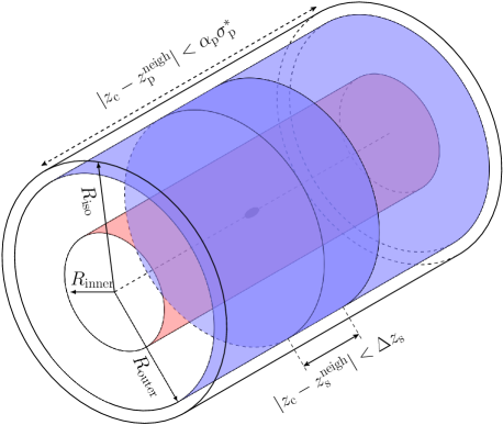
Figure 1: Schematic diagram of the sample selection procedure. For each acceptable primary, there should be no neighbouring, sufficiently bright, galaxies within a cylinder of radius $R_{\rm iso}$, centred on the primary, and nearby in redshift space. As defined in Fig. 1 in Paper I, nearby means either $|z_{\rm c}-z_{\rm s}^{\rm neigh}|<\Delta z_{\rm s}$, where $\Delta z_{\rm s}$ is the maximum allowed spectroscopic redshift difference between a primary ($\rm c$) and another galaxy ($\rm s$), or $|z_{\rm c}-z_{\rm p}^{\rm neigh}|<\alpha_{\rm p}\sigma_{\rm p}^{*}$, where $\sigma_{\rm p}$ is the measurement error of the photometric redshift and $\alpha_{\rm p}$ is the tolerance of the error, for galaxies that have no spectroscopic redshift. Satellites will lie nearby in redshift space and within the cylinder of radius $R_{\rm{inner}}$ (red), whereas the local background to be subtracted is determined from the volume between this inner cylinder and the outer one with radius $R_{\rm{outer}}$.

Our sample of isolated primary galaxies is chosen using the same criteria as in Paper I, illustrated in Fig. 1. We select primary galaxy candidates of absolute magnitude, $M_{\rm p}$, in the range $M_{\rm{C}}-\Delta M_{\rm{bin}}<M_{\rm p}\leq M_{\rm{C}}+\Delta M_{\rm{bin}}$. We then filter these primary candidates, using a series of criteria summarised in figure 1 of Paper I, to guarantee that a) there are no luminous neighbouring galaxies projected within $2R_{\rm inner}$ of the primary, unless these luminous neighbours are sufficiently separated in redshift from the primary and appear here due to a chance projection; b) the satellite search areas (projected distance $R_{\rm inner}$ from the primary) around each primary do not overlap with each other. Further details of the generation of the two samples are may be found in Paper I. The values of the selection parameters, $\{\Delta M_{\rm{bin}},\Delta M_{\rm{faint}},\Delta z_{\rm{s}},\alpha_{\rm{p}},m_{\rm v}^{\rm lim}\}=\{0.5,0.5,0.002,2.5,20.5\}$, are the same as the default values in Paper I. Here $\Delta M_{\rm{bin}}$ is the half-width of the primary magnitude $M_{\rm{c}}$ bin, $\Delta M_{\rm{faint}}$ is the magnitude difference between the primaries and satellites used to isolate primaries, $\Delta z_{\rm{s}}$ and $\alpha_{\rm{p}}$ are the parameters used to exclude galaxies that are at a significantly different spectroscopic redshift and photometric redshift respectively. The meaning of these parameters is explained in Fig. 1 (see section 2 of Paper I for more details). One small change relative to Paper 1 is that $R_{\rm{inner}}$ is chosen to increase with increasing primary luminosity, in order to ensure that no satellites are missed for the most luminous primaries.

2.2 Estimating the projected satellite number density profile

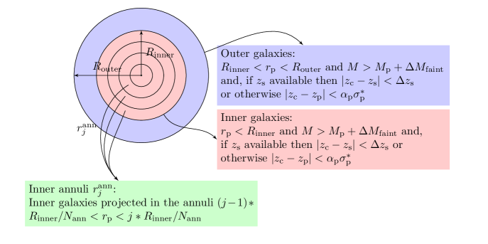
Figure 2: Schematic showing the selection of potential satellite galaxies in annuli of radii $r^{\rm ann}_{j}$ within $R_{\rm{inner}}$ and a reference sample bounded by the radii $R_{\rm{inner}}<r<R_{\rm outer}$, used to subtract the residual contaminating background. For both samples we apply the stated redshift cuts to reduce background contamination. We also apply the stated absolute magnitude cut to both samples (assuming the neighbouring galaxies are at the same redshift as the primary) though this cut is redundant unless $R_{\rm{outer}}>2R_{\rm{inner}}$ as otherwise the existence of such bright neighbouring galaxies would automatically lead to the exclusion of the primary galaxy.

Once our primary galaxies are defined, their potential satellites are found from the photometric galaxy catalogue as depicted in Fig. 2. The method we use is similar to that in Paper I, except that for each primary, the number of galaxies is counted and binned by their projected radial distances from the primary, $N(r^{\rm ann}_{j})$, as well as by their luminosity. That is, for the $i$th primary galaxy, the number of inner galaxies in each annulus, $N^{\rm{inner}}_{i}(r^{\rm ann}_{j})$, is found by counting all the neighbouring galaxies within the annulus of radius $r_{j}^{\rm ann}$ that satisfy the following conditions: at least $\Delta M_{\rm{faint}}$ fainter than the primary; if they have a spectroscopic redshift, $z_{\rm{s}}$, then they should satisfy $|z_{\rm{c}}-z_{\rm{s}}|<\Delta z_{\rm{s}}$; or if they only have a photometric redshift $z_{\rm{p}}$, then they should satisfy $|z_{\rm{c}}-z_{\rm{p}}|<\alpha_{\rm{p}}\sigma_{\rm{p}}^{*}$, where $\sigma_{\rm{p}}^{*}$ is the error in the photometric redshift as defined in Paper 1. The number of outer galaxies, $N^{\rm{outer}}_{i}$, is determined by applying the same conditions to galaxies in the outer area between $R_{\rm{inner}}$ and $R_{\rm{outer}}$. Assuming, for now, that few genuine satellites will be projected beyond $R_{\rm{inner}}$ we can estimate the surface density of genuine satellites in each annulus as

$$\Sigma^{\rm{sat}}_{i}(r^{\rm ann}_{j})=\frac{N^{\rm{inner}}_{i}(r^{\rm ann}_{j})}{A^{\rm{ann}}_{ij}}-\frac{N^{\rm{outer}}_{i}}{A^{\rm{outer}}_{i}},$$ (1)

where $A^{\rm{ann}}_{ij}$ and $A^{\rm{outer}}_{i}$ are the areas of the inner annulus and outer region respectively. If necessary, we take account of the sky coverage of SDSS DR8 by reducing the areas $A^{\rm{ann}}_{ij}$ and $A^{\rm{outer}}_{i}$ by the amounts defined by the DR7 mask described in Norberg et al. (2011).

Because of the apparent magnitude limit of SDSS, which we take to be $m^{\rm lim}=20.5$, we count the faintest satellites only at low redshift and are progressively limited to more and more luminous satellites with increasing redshift. To account for this and construct an unbiased estimate of the projected satellite number density profile over all primary galaxies, we accumulate the area contributed by the $i$th primary to the $j$th annulus for the detection of satellites brighter than $M_{\rm sat}^{\rm trun}$,

$$A_{ij}^{\rm p}(M_{\rm sat}^{\rm trun})=\left\{\begin{array}[]{ll}A_{ij}&M_{\rm sat}^{\rm trun}<M_{i}^{\rm{lim}}\\ 0&M_{\rm sat}^{\rm trun}>M_{i}^{\rm{lim}}\ .\end{array}\right.$$ (2)

Here $A_{ij}$ is the unmasked area of the $j$th annulus surrounding the $i$th primary and $M_{i}^{\rm lim}$ is the absolute magnitude that corresponds to the apparent magnitude limit, $m^{\rm{lim}}$, of the SDSS photometric catalogue at the redshift of the primary, $M_{i}^{\rm lim}=m^{\rm{lim}}-5\log_{10}(D^{L}_{i})-K(z_{i})$, where $D^{L}_{i}$ and $K(z_{i})$ are the corresponding luminosity distance and $k$-correction. This contributing area is set to zero if any potential satellites within the magnitude bin are too faint to be included, in which case we exclude this primary and its satellites as its contribution to the mean projected satellite number density profile would be incomplete. We further define $N^{\rm sat}_{ij}(M_{\rm sat}^{\rm trun})$ to be the number of detected potential satellites brighter than $M_{\rm sat}^{\rm trun}$ in the $j$th annulus surrounding the $i$th primary and $N^{\rm bck}_{i}(M_{\rm sat}^{\rm trun})$ to be the corresponding number of detected galaxies in the outer annulus, $R_{\rm{inner}}<r<R_{\rm{outer}}$, whose unmasked area is $A^{\rm outer}_{i}$. Hence we can express the mean surface density of satellite galaxies brighter than $M_{\rm sat}^{\rm trun}$ in the $j$th annulus as

$${\widetilde{\Sigma}^{\rm{sat}}(r_{j}^{\rm ann},M_{\rm sat}^{\rm trun})}=\frac{\sum_{i}N^{\rm sat}_{ij}(M_{\rm sat}^{\rm trun})}{\sum_{i}A_{ij}}-\frac{\sum_{i}N^{\rm bck}_{i}}{\sum_{i}A^{\rm outer}_{i}}.$$ (3)

In practice, we divide the projected radial distance from the primary into $20$ bins ($j=1,2,\cdots,20$). Because of a concern that the SDSS data reduction pipeline may occasionally misclassifies fragments of the spiral arms of bright galaxies as separate galaxies we exclude individual annuli that are within 1.5 times the Petrosian radius, $R_{90}$, of the primary galaxy. We set our magnitude limit, $M_{\rm sat}^{\rm trun}$, either by absolute value, such as $-20,-19,-18$, or by magnitude relative to the corresponding primary, $M_{\rm sat}^{\rm trun}=M_{\rm p}+1.0,2.0,3.0$. We present results using both thresholds so that we can determine whether the number density profiles depend on the absolute luminosity of satellites or on the relative luminosity between satellites and their primaries.

The process of estimating the projected satellite number density profiles is quite similar to estimating the satellite luminosity functions in Paper I. We divide our primaries into three luminosity bins centred on $M_{\rm{c}}=-21.25,-22.0,-23.0$. The choice of the parameters $R_{\rm{inner}}$ and $R_{\rm{outer}}$ are a balance between making them sufficiently large to avoid severely truncating the density profiles and making them too large such that our sample shrinks due to the selection process excluding overlapping systems. A sensible choice is to set $R_{\rm{inner}}$ to exceed the anticipated size of the satellite system, $r_{200}$, and $R_{\rm{outer}}$ to be roughly a factor of two larger so as to get a good, but still local, estimate of the background density. Here we have adopted the following values of $(R_{\rm{inner}},R_{\rm{outer}})$, $(0.3,0.6),(0.4,0.8)$ and $(0.55,0.9)~{}{\rm Mpc}$ for primaries in magnitude bins, $M_{\rm{c}}=-21.25,-22.0$ and $-23.0$, respectively. The values of $R_{\rm{inner}}$ have been compared with the mean of the estimated $r_{200}$ values for each galaxy in the chosen magnitude bin (see Section 3) and are found all to be larger, suggesting that the search radii for the different primary magnitude bins are sufficiently large to capture all satellites. Additional reassurance is provided by the tests in Appendix C, which show that the profiles are insensitive to changes in the values of $R_{\rm{inner}}$ or $R_{\rm{outer}}$.

2.3 Exploring the angular distribution of satellites

The projected radial satellite number density profile, $\Sigma^{\rm sat}(r)$, which is the focus of this paper, is the azimuthal average of the 2D surface density, $\Sigma^{\rm sat}(r,\theta)$, where $\theta$ can be taken as the position angle between the major axis of the primary and the line connecting the primary and satellite (see Fig 3). The angular dependence of this distribution may also carry information on the formation and evolution of the satellites around their primaries. For example, if we assume that the satellite galaxies inhabit an unbiased set of dark matter subhalos, then we would expect satellites to cluster preferentially along the major axis of the halo (Libeskind et al., 2005). Moreover, it is known that the host halos of satellite systems are accreted from filaments, which can cause the angular distribution of satellites around primaries to be anisotropic (Hartwick, 2000). In fact, numerous such anisotropies have been observed. For example, the famous “Holmberg Effect” (Holmberg, 1969), suggests satellites of isolated, large, and inclined spiral galaxies are preferentially located along the minor axes of their primaries, a result supported by Zaritsky et al. (1997b). However Yang et al. (2006), Azzaro et al. (2007), Brainerd (2005) and Agustsson & Brainerd (2011) found the opposite effect that satellites prefer alignment with the major axis, especially for the satellites of red primaries. Since the direct observation of satellite systems is not easy, the sample of external satellite systems is limited in both volume and quality. These contradictory results may suggest that the mean amplitude of the anisotropy could be very weak, or the form of the anisotropy could be dependent on the selection of the primaries or even the satellites themselves.

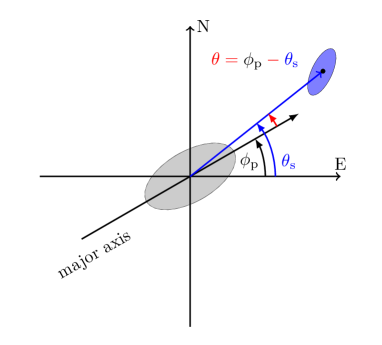
Figure 3: Schematic showing the definition of the position angle $\theta$ which characterises the angular position of the satellite relative to the direction of the primary galaxy’s major axis. The grey and blue ellipses are the primary and satellite galaxy, respectively. The angle $\phi_{\rm p}$ is the position angle of the primary.

It is therefore interesting to attempt to quantify the mean anisotropy of our large sample of satellite galaxies. We characterise the angular distribution using the position angle $\theta$ described in Fig. 3. The assumed elliptical symmetry of the primary implies that $\theta$ ranges from $0^{\circ}$ to $90^{\circ}$ with these extremes indicating that the satellites are located along the major or minor axis respectively. The anisotropy of the angular distribution is then quantified by the probability distribution of the angle $\theta$. In practice, accurate measurement of $\theta$ requires a robust measurement of the position angle $\phi_{\rm p}$ defining the orientation of the primaries. To achieve this, we adopt the same selection criteria as Siverd, Ryden, & Gaudi (2009). We only select primaries and their satellites that satisfy the condition, $q_{\rm iso}<0.9$ and $q_{\rm mom}<0.9$, where $q_{\rm iso}$ is the isophotal axis ratio defined as $q_{\rm iso}=a_{\rm iso}/b_{\rm iso}$ and $q_{\rm mom}$ is the adaptive moments axis ratio, $q_{\rm mom}=((1-e)/(1+e))^{1/2}$ where $e=(e^{2}_{+}+e^{2}_{\times})^{1/2}$ (Ryden, 2004). We also exclude the primaries together with their satellites if there is a discrepancy of more than $15$ degrees between the measured isophotal and de Vaucouleurs position angles, $\Delta\theta_{\rm p}^{\rm iso-mod}>15^{\circ}$.

For our sample of selected satellite systems, the number of satellites located at angle $\theta_{j}$ around the $i$th primary, can be estimated as

$$N^{\rm sat}_{i}(\theta_{j})=N_{i}^{\rm inner}(\theta_{j})-\frac{A^{\rm{inner}}_{i}}{A^{\rm{outer}}_{i}}\left\langle N_{i}^{\rm outer}(\theta_{j})\right\rangle,$$ (4)

where $\left\langle N_{i}^{\rm outer}(\theta_{j})\right\rangle$ represents the azimuthal average as we assume the background galaxies are, on average, isotropically distributed. Note that to avoid biasing the angular distribution we exclude systems that are incomplete due to the survey mask. We can then define an unbiased estimator of the average distribution of the satellite position angle $\theta$ for all selected primaries as

$$\widetilde{N}(\theta_{j},M_{\rm sat}^{\rm trun})=\frac{\sum_{i}N^{\rm sat}(\theta_{j},M_{\rm sat}^{\rm trun})}{N_{j}^{\rm prim}(M_{\rm sat}^{\rm trun})}.$$ (5)

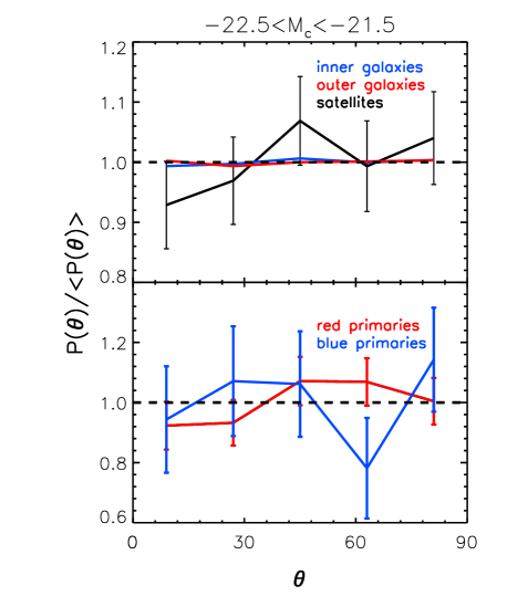
Figure 4: The probability distribution, $P(\theta)$, of the position angle $\theta$ of satellite galaxies. In the top panel the blue and red lines show the distributions, $P^{\rm inner}(\theta)$, of inner galaxies, and $P^{\rm outer}(\theta)$, of outer galaxies, respectively. The inferred distribution for true satellite galaxies, $\widetilde{P}^{\rm sat}(\theta)$, is shown by the black line. The lower panel shows the distributions for red and blue primary subsamples, as the red and blue solid lines respectively. The error bars are calculated from $1000$ bootstrap resamplings. The expectation for a uniform distribution is shown by the dashed lines in the two panels.

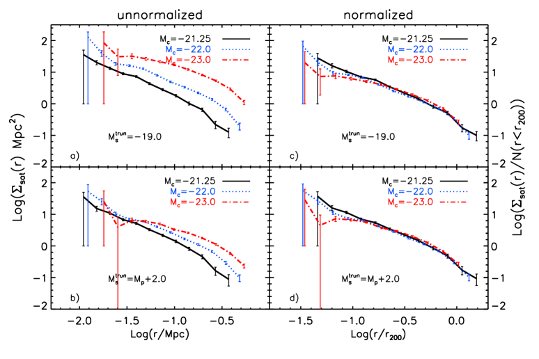
Figure 5: The mean projected number density profiles of satellites around primaries for various selections of primaries and satellites. The left hand panels (a and b) show the mean number densities and the right hand panels (c and d) show the same profiles but now normalized by the total number of satellites within the $r_{200}$ radius (see right-hand axis) and with the radius expressed in units of the adopted mean $r_{200}$ radius of the primaries. In each panel the different coloured lines correspond to primaries of differing luminosity as indicated in the legend. The profiles in the upper panels (a and c) are for satellite samples brighter than $M_{\rm sat}^{\rm trun}=-19$, while the lower panels (b and d) are for satellites that are less than 2.0 magnitudes fainter than their respective primaries. The error bars show the errors on the mean profiles estimated by bootstrap resampling.

The normalized probability distribution of $\theta$ for primaries in the magnitude bin $M_{\rm{c}}=-22.0$ is shown in Fig. 4. The blue, red and black solid lines in the top panel are the probability distributions of $\theta$ for inner galaxies, $P^{\rm inner}(\theta)$, outer galaxies, $P^{\rm outer}(\theta)$, and that inferred for satellite galaxies, $\widetilde{P}(\theta)$, respectively. In the bottom panel of Fig. 4, we show the probability distribution of $\theta$ for two satellite subsamples split by rest frame colour of their primary galaxies. These samples are divided according to the well-known colour bimodality in the colour-magnitude plane (e.g. Strateva et al., 2001; Baldry et al., 2004; Zehavi et al., 2005). Following Zehavi et al. (2005), we use an equivalent colour criterion of ${}^{0.0}(g-r)_{\rm{cut}}=0.19-0.24M_{r}$ (not identical to Zehavi et al. as our magnitudes are $k$-corrected to $z=0.0$ rather than $z=0.1$). The probability distributions of $\theta$ in Fig. 4 are all consistent with isotropic distributions. This is confirmed by a two-sample Kolmogorov-Smirnov (KS) test that compares the distributions of inner and outer galaxies for the whole primary sample and also the subsamples of red and blue primaries. The two-sample KS probabilities from the whole sample, blue and red primary subsamples are $0.64,0.37,0.87$ respectively, which implies that the pairs of distributions have no statistically significant differences. The same tests for primaries in other magnitude bins show similar results.

Therefore, with our satellite system sample, we find that there is no statistically significant evidence that the distribution of satellites around primaries is anisotropic. This could signify that the anisotropy of the distribution of satellites around isolated primaries is intrinsically insignificant. However, one also has to keep in mind that our inner sample includes contamination from interlopers, because these are only rejected using inaccurate photometric redshifts, and this could dilute any intrinsic anisotropy signal.

3 Results

We now return to the azimuthally averaged density profiles. Density profiles for satellites brighter than $M_{\rm sat}^{\rm trun}$ around primaries of magnitude $M_{\rm c}$ are shown in Fig. 5 for a variety of primary magnitude bins and satellite magnitude cuts. Panels 5a and 5b show that the number of satellites increases with increasing primary luminosity and extends to larger radii. To investigate the variation in profile shape between different subsamples of satellites and primaries, it is helpful to use scaled variables. To this end, we recast the profiles in terms of $x=r/r_{200}$ and divide the number densities by the total number of satellites within $r_{200}$.

The values of $r_{200}$ used to scale the radii can be determined from the stellar masses, themselves inferred from the measured galaxy luminosities and colours, and the abundance matching technique of Guo et al. (2010), which gives

$$\frac{M_{*}}{M_{\rm halo}}=c\left[\left(\frac{M_{\rm halo}}{M_{0}}\right)^{-\alpha}+\left(\frac{M_{\rm halo}}{M_{0}}\right)^{\beta}\right]^{-\gamma},$$ (6)

where $c=0.129$, $M_{0}=10^{11.4}~{}\rm{M_{\sun}}$, $\alpha=0.926$, $\beta=0.261$ and $\gamma=2.440$ are fitted constants. The halo mass can be related to a radius through

$$M_{\rm halo}=\frac{4\pi}{3}200\rho_{\rm crit}r^{3}_{\rm 200}.$$ (7)

Figure 6: The dependence of the scaled satellite density profiles on satellite luminosity for primaries in the magnitude range $-22.5<M_{\rm p}<-21.5$. The different panels show different satellite selections. The upper panels, which are very similar, show profiles for satellites brighter than a threshold that is either a fixed value (panel a) or specified as a magnitude difference with respect to the corresponding primary (panel c; see legend). The lower two panels show profiles for satellites in bands of magnitude again either specified between fixed values (panel b) or between values relative to the corresponding primary (panel d).

For the primary galaxies there is a significant uncertainty in the stellar mass that is inferred from the measured luminosities and colours. Thus, rather than using the individual $r_{200}$ values to normalise satellite number density profiles for each primary before stacking them together, the mean $r_{200}$ for all primaries in the luminosity bin of interest is determined and a single rescaling is performed on the unscaled, stacked profile. Using $r_{200}$ values determined in this way, the $M_{c}=-21.25$ and $-22.0$ samples line up very well, as shown in panels 5c and 5d. However, the $M_{c}=-23.0$ results, not shown in Fig. 5, are slightly offset. For these, the most luminous primaries, the relation between stellar mass and halo mass becomes very flat and there is a large spread in the halo mass corresponding to a given stellar mass. This makes the assignment of a value of $r_{200}$ to these primaries extremely uncertain. The directly inferred virial radius is 0.73 Mpc but we find that a smaller value of 0.52 Mpc results in better scalings. Given the large uncertainty in this assignment, it is not unreasonable to adopt this smaller value. We shall do this in what follows but this uncertainty must be borne in mind when interpreting the results for the brightest primary bin. The final values of $r_{200}$ for the three primary magnitude bins are $0.24,0.37,0.52~{}{\rm Mpc}$, the first two of which come directly from equation (7). By adopting these mean $r_{200}$ values, we have a mass-to-light ratio increasing with luminosity as $M/L_{V}\propto L_{V}^{0.42}$. This is similar to the relation found by Prada et al. (2003), albeit for the B-band, from a set of spectroscopically selected satellites from SDSS. For $M_{V}$ =-22, we find that $M/L_{V}$=140.

First, we explore the dependence of the normalized profiles on the luminosity of the satellites. In Fig. 6, we show normalized profiles for primaries of fixed luminosity ($-22.5<M_{\rm p}<-21.5$) with a variety of different satellite selections. In all cases we find the outer shapes of the density profiles to be very similar. The only variation is on small scales (roughly $r/r_{200}<0.1$) where the density profile is steeper and higher for the faintest satellites.

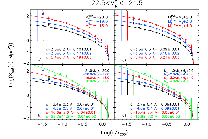
Figure 7: Fits to the satellite density profiles of primaries of magnitude $-22.5<M_{\rm p}<-21.5$ using projected, background-subtracted NFW profiles. The various panels show different selections of satellites as in Fig. 6, except that here we have not normalized the profiles, but instead allowed the amplitude, $A$, of the fitted profiles to float. The measured profiles are shown by the data points and the best fitting NFW profiles are plotted as solid lines. The best fitting amplitudes and concentrations are listed in the legends in each panel.

We examine the shape of these density profiles more systematically in Fig. 7 where we fit the unnormalized density profiles using an analytic model. We have chosen to fit our satellite profiles using NFW profiles as they are known to be good fits to both dark matter haloes (Navarro, Frenk, & White, 1996, 1997) and to the distribution of substructures within them (Diemand, Moore, & Stadel, 2004; Springel et al., 2008; Ludlow et al., 2009). To perform these fits we first project the NFW profile and subtract from it the mean density in an outer “background” annulus as described in Appendix A, so as to match the background subtraction process that we have applied to our observational data. We then perform a fit using $\Sigma^{\rm sat}(r)=A\hat{\Sigma}(r,c,r_{\rm 200})/M_{\rm 200}$, where $A$ is a scale factor, $c$ is the concentration, and $\hat{\Sigma}(r,c,r_{\rm 200})$ is the projected NFW profile with background subtracted as given in Eqn. 18. The $r_{200}$ radius is fixed to the respective values that we have adopted for each of our bins of primary magnitude.

Fig. 7 shows the resulting fits. The bright satellites, such as satellites with magnitudes $-21.0<M_{s}<-20.0$ or $M_{\rm p}+1.0<M_{s}<M_{\rm p}+2.0$ are very well fitted by the projected and background subtracted NFW profiles. The NFW fits also remain good descriptions of the data for the cumulative samples of satellites defined by a faint magnitude threshold. For these samples, shown in the upper panels of Fig. 7, the concentration increases steadily with decreasing luminosity. In the lower panels of Fig. 7, which show density profiles for satellites in differential bands of luminosity, we see both a stronger dependence of concentration on luminosity and small deviations from the NFW form for the faintest satellite samples.

We now turn to the dependence of the satellite profiles on the magnitude of the primaries. In Fig. 8 we show fits of the projected and background-subtracted NFW profiles to satellite profiles of primaries in each of our three magnitude bins. Each of the panels corresponds to a different selection of satellites. We see that NFW fits are good descriptions of the satellite distribution regardless of the luminosity of the primary. The right hand panels of Fig. 8 show the density profiles and fits for sets of satellites defined by fixed offsets in magnitude from the magnitude of their respective primary. If the combined primary and satellite systems scaled in a self-similar way we would expect the three density profiles in each of these panels to lie on top of each other. In contrast, in each panel, we see systematic variations in the shape and amplitude of the profiles with the primary luminosity. If instead we look at the left hand panels, which show satellites selected in different fixed magnitude bands, then we see that the concentration decreases steeply with increasing satellite luminosity, but is less dependent on the luminosity of the primary. With the exception of the brightest primary magnitude bin ($M_{\rm{c}}=-23.0$), the satellites of a given luminosity are more or less distributed in the same way about primaries of different luminosity. Only the normalization of the profile, as parameterized by $A$, increases with increasing primary luminosity. This depends quite strongly on luminosity going roughly as the luminosity to the power of $2.5$. If we normalized each of these satellite profiles as we did in Fig. 6, then their shapes would show very little variation with primary luminosity.

For the case of primaries in the $M_{\rm{c}}=-23.0$ bin, the measured concentrations for the satellite distributions are systematically lower than those of similar luminosity satellites around less luminous primaries. The reason for this is not clear. It may be that this result reflects the actual satellite distribution around bright primaries. However, it could be an artefact of the estimation procedure. One possibility is that the non-linearity of the halo mass-stellar mass relation (Guo et al., 2010) means that the range of actual halo mass increases in the brightest primary bin. Thus, stacking all primaries using a single $r_{200}$ value may be introducing errors that would smear out the resulting profile. Another potential source of systematic error comes from the tendency for faint satellites to be missed around bright primaries because of inaccuracies in the sky-subtraction (Mandelbaum et al., 2005). Even with the updated sky-subtraction algorithm employed for DR8 there may still be some residual loss of faint satellites around the brightest primary galaxies (Aihara et al., 2011).

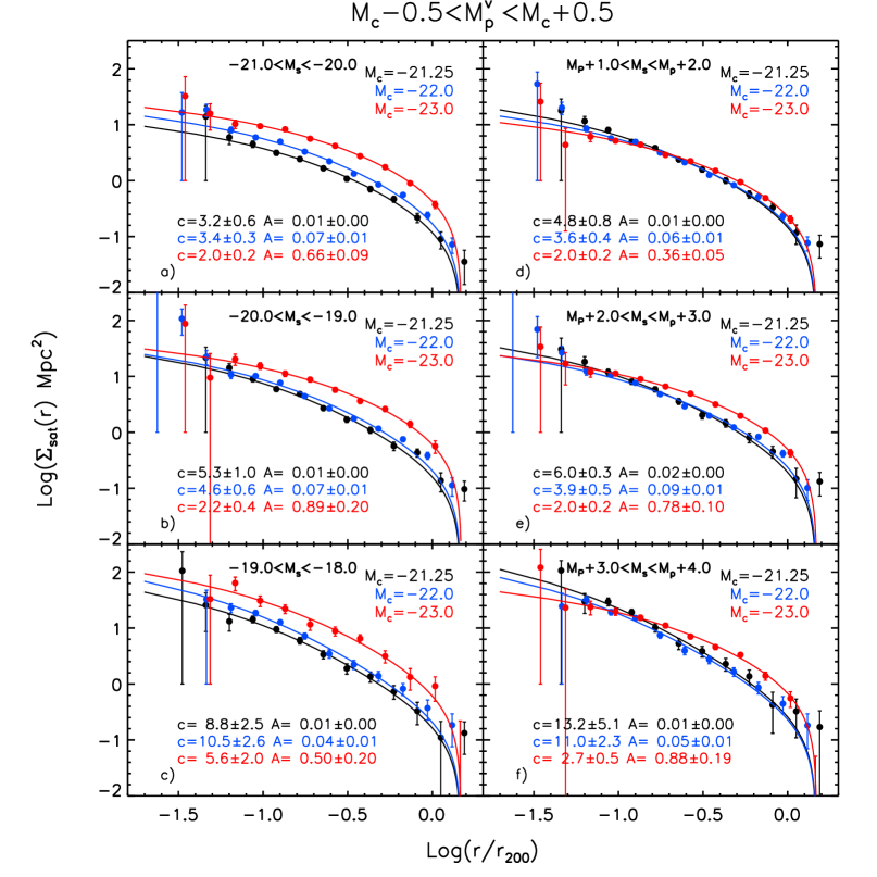
Figure 8: NFW fits to the density profiles of satellites around primaries of different luminosity. Each panel shows fits for the three different bins of primary luminosity indicated in the legends. The different panels correspond to different selections of satellites. The panels on the left, a), b) and c), are for successively fainter bands of satellite luminosity as indicated on the legend, with the range of satellite magnitudes being the same for each primary. In contrast the panels on the right, d), e) and f), are for bins of satellite magnitude that are specified as an offset relative to the magnitude of their respective primary.

3.1 Colour and type dependence

Our large sample of satellite systems enables us to divide our samples by the colour or the type of the primaries. Fig. 9 shows the resulting profiles when primaries of $V$-band magnitude $-22.0\pm 0.5$ are split by colour and by concentration. Panels a) and c) of Fig. 9 show that the normalized profile of satellites around blue primaries is more concentrated than that around red primaries. Panels b) and d) split the sample into early and late types, where early type is defined as having a concentration index $\mathcal{C}\equiv{petroR_{90}}/{petroR_{50}}\geq 2.6$, with $petroR_{90}$ and $petroR_{50}$ being the SDSS Petrosian 90% and 50% light radii respectively. This division roughly separates early type (E/S0) from late-type (Sa/b/c, Irr) galaxies (Shimasaku et al., 2001). We also see the amplitude of the profiles of late types is suppressed with respect to that of the early types. However, the concentration indices, $c$, from the fits similarly show that the concentration of satellites around late types is higher than that of early types.

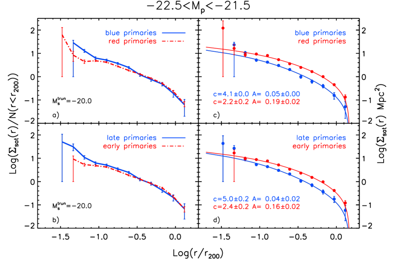
Figure 9: The satellite profiles for primary galaxies of magnitude $-22.5<M_{\rm p}<-21.5$ split by the type (concentration) and colour of the primary. Panels a) and b) show the normalized profiles while panels c) and d) show NFW fits to the unnormalized profiles (see right hand axis). In the upper panels the blue lines refer to blue primaries and red lines to red primaries, while in the lower panels blue refers to late-type primaries and red to early types.

We can also use the colour information available in SDSS to probe the properties of the satellites. Firstly, for the bin of primary magnitude, $M_{\rm{c}}=-22.0$, we divide the satellites into two luminosity bins, $-21.0<M_{\rm s}<-20.0$ and $-20.0<M_{\rm s}<-19$ and into red and blue subsamples using the same cut as before. Fig. 10a,b,d and e show the measured profiles of these blue and red satellites and NFW fits. We first note from Fig. 10d and e that for these relatively bright satellite samples the abundance of blue satellites is greater than that of red satellites at all radii, with this difference increasing for the fainter sample. The profiles of the brighter satellites have a similar shape for red and blue satellites, while the fainter red satellites have an excess at $\sim 0.1r_{200}$ relative to the fainter blue satellites. To investigate whether these differences are driven by the colours of the associated primary galaxies we further split the satellites brighter than $M_{\rm s}^{\rm trun}<-20$ by the colour of their primary. The results are shown in Fig. 10c and f. Both red and blue primaries have more blue than red satellites. The concentrations of red and blue satellites around blue primaries are similar. Red primaries have lower concentrations for both their red and blue satellites, with the blue satellites having a particularly low concentration. The colour of the primary appears to be more important than that of the satellite in determining the concentration of the satellites. As shown in Fig. 8, the satellite luminosity also has a strong effect.

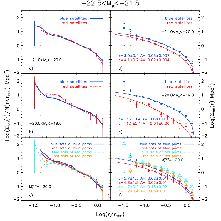
Figure 10: Satellite density profiles split by the colour and luminosity of the satellites. Panels a) and b) compare the profiles of blue (blue solid line) and red (red dot-dashed line) satellites for two different bins of satellite luminosity (see legend). Panels d) and e) show the corresponding unscaled profiles as red and blue symbols together with curves depicting NFW fits. The best fitting amplitudes and concentrations are given in the legends. For satellites brighter than -20.0, panels c) and f) compare the profiles of red and blue satellites around red and blue primaries. The profiles for blue primaries are shown with solid lines and those for red primaries with dashed lines. The blue and cyan lines are for blue satellites and red and orange lines for red satellites as detailed in the legends. In panel f) the smooth curves show the NFW fits to the corresponding unscaled profiles and again the best fit parameters are listed in the legend.

4 Discussion

Using a stacking analysis we have estimated the mean projected density profiles of satellite galaxies around a large sample of isolated primary galaxies selected from the SDSS DR8 spectroscopic galaxy catalogue and we have quantified how they depend on the properties of the satellites and primaries. The selection of primaries and the local background subtraction technique, which makes use of photometric redshifts, is the same as in Paper I (Guo et al., 2011) where we estimated the mean satellite luminosity functions of these systems. Our main conclusions are:

(i) We find no evidence for any anistropy in the satellite galaxy distribution relative to the major axes of the primaries.

(ii) The projected number density profiles of satellites brighter than a $V$-band magnitude of $-17$ are well determined for three separate bins of primary magnitude, $-21.25,-22,0,-23.0$.

(iii) Apart from the faintest satellites, for which there is a slight excess at small galactocentric projected distance, all other density profiles are well fitted by projected NFW profiles that have been background subtracted to match the procedure that has been applied to the data.

(iv) The concentration of the NFW fits decreases systematically with increasing satellite luminosity and is almost independent of the luminosity of the primaries (see Fig. 8). Thus, bright satellites have more extended distributions and fainter satellites are more centrally concentrated.

(v) The radial distribution of satellites is dependent on the colour and morphology of their primaries. Satellites are more numerous around red/early primaries and have more extended, lower concentration, distributions (see Fig. 9).

(vi) The radial distribution of satellites also depends on the colour of the satellites. Blue satellites are more numerous than red satellites at all radii (for the luminosity range we probe) and faint red satellites are more centrally concentrated (higher NFW concentration) than faint blue satellites. Further sub-divided samples show that the concentration of the blue or red satellite profile depends more on the colour of the primaries than it does on the colour of the satellites.

As a check of potential systematic effects in our results, we have also performed the same analysis using the SDSS DR7 dataset. Generally, the results based on DR7 are consistent with those from DR8, although we do observe some differences in the distribution of faint satellites. This is most likely due to less accurate photometric reduction and sky-background subtraction for DR7 (see Appendix B for more details).

With the advantage of our large and carefully selected samples, we have discovered a variety of interesting information about the projected number density profiles, which it has not been possible to quantify clearly in previous work. However, even with a very limited sample, a pioneering study by Lorrimer et al. (1994) found that the distribution of satellites is dependent on the morphology of primaries. They found that the number of satellites around early-type primaries is greater than that about late-type primaries and that the concentration of the satellite distribution is higher around early type primaries. We confirm the greater abundance of satellites around early-type primaries, but contrary to Lorrimer et al. (1994) we find higher concentrations for satellite systems around late-type primaries. More recently, van den Bosch et al. (2005), Sales & Lambas (2005) and Chen et al. (2006) studied the projected number density profiles of satellites of isolated galaxies using larger samples from the Two Degree Field Galaxy Redshift Survey (2dFGRS) and SDSS. Although van den Bosch et al. (2005) cautioned that the profiles from 2dFGRS were incomplete because of incompleteness in close galaxy pairs, their study revealed that satellites followed NFW profiles. Sales & Lambas (2005) found that the profiles of satellites depart from a power law at small galactocentric projected distance, and that they are dependent on the colour of the primaries, which is similar to our conclusions (iv) and (v). They also found the distribution of satellites to depend on their colour, but argued that this may be caused by the correlation between satellites and primaries. In our study, conclusion (vi) shows that the distribution of satellites not only depends on the properties of satellites, but also depends on the colour of primaries. Chen et al. (2006) and Tollerud et al. (2011) selected samples only from the SDSS spectroscopic catalogue in their studies. Tollerud et al. (2011) found the 3D number density profiles of satellites can be fitted by a power-law with a slope $\rho\propto r^{-1.8}$. After projecting, the slope of this density profile will be close to ours. With a careful treatment of interlopers, they fitted the profiles with a power-law form and found them to be independent of the luminosity of the primaries. These conclusions are consistent with ours. Very recently, Lares, Lambas, & Domínguez (2011) estimated the radial density profiles of satellites around primary samples brighter than $-20.5$ and $-21.5$. They also found the amplitudes of the profiles depend on the luminosity of the primaries, and the shapes on their colour.

The physics of the projected number density profiles of satellites involves both the physics of the hierarchical assembly of dark matter halos and the physics of the galaxy formation that occurs in these assembling halos. Hence quantifying these profiles will help constrain both galaxy formation models and the nature of the dark matter. We expect that our profile results and those of others will be an important input into refining theoretical models and the next incarnation of full N-body/gasdynamic simulation that can resolve the physics of the formation of satellite galaxies.

Appendix A The Projected NFW Profile with background subtraction

The NFW density profile (Navarro, Frenk, & White, 1996, 1997) is

$$\rho(r)=\frac{\delta_{\rm c}\rho_{\rm c}}{(r/r_{\rm s})(1+r/r_{\rm s})^{2}},$$ (8)

where $\rho_{\rm c}$ is the critical density, $\delta_{\rm c}$ is the characteristic overdensity of the halo and $r_{\rm s}$ is a characteristic scale length. Conventionally, the scale length is specified in terms of a concentration defined as $c=r_{\rm 200}/r_{\rm s}$, where the $r_{200}$ radius is defined as the radius at which the mean interior density is $200\rho_{\rm c}$. With these definitions it follows that

$$\delta_{c}=\frac{200}{3}\frac{c^{3}}{\ln(1+c)-c/(1+c)}.$$ (9)

We can integrate along a line of sight to obtain the projected surface mass density

$$\Sigma(R)=2\delta_{\rm c}\rho_{\rm c}r_{\rm s}\int_{R}^{\infty}\frac{1}{\sqrt{r^{2}-R^{2}}\,(r/r_{\rm s})\,(1+r/r_{\rm s})^{2}}{\rm d}r,$$ (10)

where $R$ is the projected distance from the centre of the halo. This integral can be solved analytically (Bartelmann, 1996) and expressed as

$$\Sigma(x)=\left\{\begin{array}[]{ll}\frac{\displaystyle{2\delta_{\rm c}\rho_{\rm c}r_{\rm s}}}{\displaystyle{(x^{2}-1)}}\left[\displaystyle{1-\frac{2}{\sqrt{(1-x^{2})}}{\rm arctanh}\sqrt{\frac{1-x}{1+x}}}\right]&\\ \hskip 142.26378ptx<1,&\\ \displaystyle{\frac{2\delta_{\rm c}\rho_{\rm c}r_{\rm s}}{3}}\hskip 110.96556ptx=1,&\\ &\\ \displaystyle{\frac{2\delta_{\rm c}\rho_{\rm c}r_{\rm s}}{(1-x^{2})}}\left[\displaystyle{1-\frac{2}{\sqrt{(x^{2}-1)}}{\rm arctan}\sqrt{\frac{x-1}{1+x}}}\right]&\\ \hskip 142.26378ptx>1,&\end{array}\right.$$ (17)

where $x=R/r_{s}$. In our profile measurements, we remove the contamination of interlopers by subtracting the mean density of galaxies in an outer annulus. This outer annulus will also contain genuine satellites that are in the outer annulus of the density profile. Hence, to compare fairly with the measured profiles, we should apply the same background subtraction process to the projected NFW profile. We denote the resulting background-subtracted projected NFW profile as

$$\hat{\Sigma}(x)=\Sigma(x)-\frac{2r_{s}^{2}}{3r_{200}^{2}}\int_{x_{200}}^{2x_{200}}\Sigma(x)\,x\,{\rm d}x.$$ (18)

These background-subtracted profiles are compared to their unsubtracted counterparts in Fig. 11. The subtracted profiles tend to zero at projected $R/r_{200}\sim 1.4$.

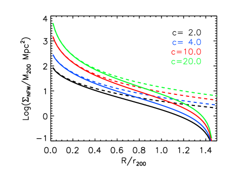
Figure 11: A comparison of projected NFW profiles (dashed lines) and background-subtracted projected NFW profiles (solid lines) for different values of the concentration, $c$. The projected radius, $R$, is expressed in units of the $r_{200}$ radius, $r_{200}$.

Appendix B Comparison of results from DR8 with DR7

We have performed our measurement of satellite number density profiles for both the SDSS DR8 and DR7. This helps to quantify the impact on the number density profiles of the different sky-subtraction algorithms used to define these galaxy catalogues. Looking at images of some of our primary galaxies in DR7, there were occasions when close-in satellite galaxies existed that were not present in DR8. The suggestion is that these are spurious fragments of the primary galaxy itself, following inexact subtraction of the background sky level. One would expect such a problem to be worse for lower luminosity satellites and also if the inner radius cut to be considered is reduced beyond our default 1.5 times the Petrosian $R_{90}$. Fig. 12 shows some illustrative results where satellites down to 0.5 times the Petrosian $R_{90}$ have been included in the profiles around $M_{\rm{c}}=-23.0$ primaries. There is a tendency for DR7 to have extra low luminosity satellites near to the primary, which is not shared by DR8. This is particularly evident in the lower panel. Furthermore, while the DR8 profile is robust to changing the inner radius cut, the result for the low luminosity satellite profile around bright primaries from DR7 changes significantly. We conclude that DR7 contains more spurious fragmentation of bright primary galaxies, and that DR8 is preferable for our study, both in terms of the reliability of the faint galaxies and their improved photometry.

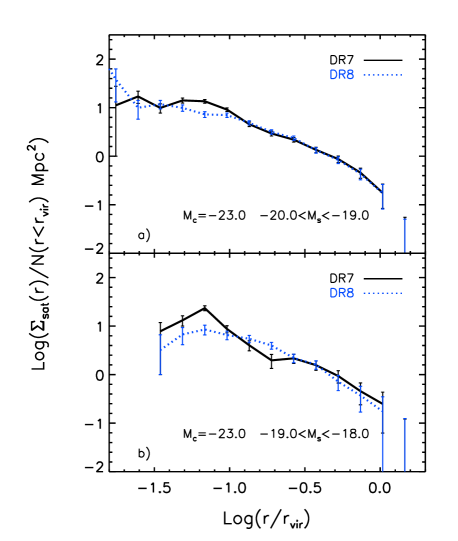
Figure 12: A comparison of profiles based on SDSS DR8 and DR7 for a) more luminous satellites, and b) less luminous satellites. The black (solid) lines are the profiles from DR7. The blue (dotted) lines are the profiles from DR8. A cut at 0.5 times the Petrosian $R_{90}$ radius is used to highlight the difference.

Appendix C Validation of the satellite search parameters

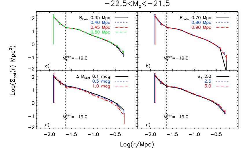
Figure 13: The effect on the estimated number density profiles of varying the parameters {$R_{\rm{inner}},R_{\rm{outer}},\Delta M_{\rm{faint}},\alpha_{\rm{p}}$} from their default values, {0.3 Mpc,0.6 Mpc,0.5,2.5}, as indicated in the legends. Some error bars for different datasets have been slightly shifted for clarity.

In Fig. 13, we show the effect on the estimated number density profiles of varying various satellite search parameters. Panel (a) demonstrates that varying $R_{\rm inner}$ between 0.35 and 0.50 Mpc does not change the profiles significantly, because $R_{\rm inner}=0.35$ Mpc is already large enough to enclose the whole satellite system for primaries satisfying $-22.5<M_{\rm p}<-21.5$. The satellite number density profile is similarly robust to changes in $R_{\rm{outer}}$, which is the outer radius for the background region, as shown in panel (b). The next panel shows the effect of varying $\Delta M_{\rm{faint}}$, the parameter used to determine if a primary is isolated. There is a very weak variation of the profile shown in panel (c), with primaries allowed to have neighbours with a magnitude difference as small as $\Delta M_{\rm{faint}}=0.1$ having slightly more satellites than those with larger magnitude differences to their neighbours, more in keeping with the term isolated. Besides the physically motivated parameters, we also test the parameters of the estimation method. The parameter $\alpha_{\rm{p}}$ helps us to distinguish genuine satellite galaxies from background galaxies by excluding galaxies that are at a significantly different redshift. Panel (d) shows that our results are insensitive to reasonable changes in the value of $\alpha_{\rm{p}}$.

References

- (1)
- Agustsson & Brainerd (2010) Agustsson I., Brainerd T. G., 2010, ApJ, 709, 1321
- Agustsson & Brainerd (2011) Agustsson I., Brainerd T. G., 2011, arXiv, arXiv:1110.5920
- Aihara et al. (2011) Aihara H., et al., 2011, ApJS, 193, 29
- Azzaro et al. (2007) Azzaro M., Patiri S. G., Prada F., Zentner A. R., 2007, MNRAS, 376, L43
- Belokurov et al. (2008) Belokurov V., Walker M. G., Evans N. W., et al., 2008, ApJ, 686, L83
- Benson et al. (2002) Benson, A. J., Frenk, C. S., Lacey, C. G., Baugh, C. M., & Cole, S. 2002, MNRAS, 333, 177
- Baldry et al. (2004) Baldry I. K., Glazebrook K., Brinkmann J., Ivezić Ž., Lupton
- Bartelmann (1996) Bartelmann M., 1996, A&A, 313, 697
- Brainerd (2005) Brainerd T. G., 2005, ApJ, 628, L101 R. H., Nichol R. C., Szalay A. S., 2004, ApJ, 600, 681
- Blanton & Roweis (2007) Blanton M. R., Roweis S., 2007, AJ, 133, 734
- Bullock, Kravtsov & Weinberg (2000) Bullock, J. S., Kravtsov, A. V. & Weinberg, D. H.2000, ApJ, 539, 517
- Busha et al. (2010) Busha M. T., Alvarez M. A., Wechsler R. H., Abel T., Strigari L. E., 2010, ApJ, 710, 408
- Chen et al. (2006) Chen J., Kravtsov A. V., Prada F., Sheldon E. S., Klypin A. A., Blanton M. R., Brinkmann J., Thakar A. R., 2006, ApJ, 647, 86
- Colless et al. (2001) Colless M., et al., 2001, MNRAS, 328, 1039
- Cooper et al. (2010) Cooper A. P., et al., 2010, MNRAS, 406, 744
- Diemand, Moore, & Stadel (2004) Diemand J., Moore B., Stadel J., 2004, MNRAS, 352, 535
- Font et al. (2011) Font A. S., et al., 2011, arXiv, arXiv:1103.0024
- Grebel (2000) Grebel E. K., 2000, in Star Formation from the Small to the Large Scale, edited by F. Favata, A. Kaas, A. Wilson, vol. 445 of ESA Special Publication, 87
- Guo et al. (2010) Guo Q., White S., Li C., Boylan-Kolchin M., 2010, MNRAS, 404, 1111
- Guo et al. (2011) Guo Q., Cole S., Eke V., Frenk C., 2011, MNRAS, 417, 370
- Hartwick (2000) Hartwick F. D. A., 2000, AJ, 119, 2248
- Holmberg (1969) Holmberg E., 1969, ArA, 5, 305
- Irwin et al. (2007) Irwin M. J., Belokurov V., Evans N. W., et al., 2007, ApJ, 656, L13
- Kim et al. (2011) Kim E., Kim M., Hwang N., Lee M. G., Chun M.-Y., Ann H. B., 2011, MNRAS, 412, 1881
- Klypin et al. (1999) Klypin, A., Kravtsov, A. V., Valenzuela, O., & Prada, F. 1999, ApJ, 522, 82
- Klypin, Zhao, & Somerville (2002) Klypin A., Zhao H., Somerville R. S., 2002, ApJ, 573, 597
- Klypin & Prada (2009) Klypin A., Prada F., 2009, ApJ, 690, 1488
- Kauffmann et al. (1993) Kauffmann, G., White, S. D. M., & Guiderdoni, B. 1993, MNRAS, 264, 201
- Koposov et al. (2008) Koposov, S., et al. 2008, ApJ, 686, 279
- Koposov et al. (2009) Koposov, S. E., Yoo, J., Rix, H.-W., Weinberg, D. H., Macciò, A. V.; Escudé, J. M. 2009, ApJ, 696, 2179
- Lake & Tremaine (1980) Lake G., Tremaine S., 1980, ApJ, 238, L13
- Lares, Lambas, & Domínguez (2011) Lares M., Lambas D. G., Domínguez M. J., 2011, AJ, 142, 13
- Li et al. (2007) Li C., Jing Y. P., Kauffmann G., Börner G., Kang X., Wang L., 2007, MNRAS, 376, 984
- Li, De Lucia, & Helmi (2010) Li Y.-S., De Lucia G., Helmi A., 2010, MNRAS, 401, 2036
- Libeskind et al. (2005) Libeskind N. I., Frenk C. S., Cole S., Helly J. C., Jenkins A., Navarro J. F., Power C., 2005, MNRAS, 363, 146
- Libeskind et al. (2007) Libeskind, N. I., Cole, S., Frenk, C. S., Okamoto, T., Jenkins, A. 2007, MNRAS, 374, 16L
- Liu et al. (2008) Liu C., Hu J., Newberg H., Zhao Y., 2008, A&A, 477, 139
- Lorrimer et al. (1994) Lorrimer S. J., Frenk C. S., Smith R. M., White S. D. M., Zaritsky D., 1994, MNRAS, 269, 696
- Lovell et al. (2011) Lovell M., et al., 2011, arXiv, arXiv:1104.2929
- Ludlow et al. (2009) Ludlow A. D., Navarro J. F., Springel V., Jenkins A., Frenk C. S., Helmi A., 2009, ApJ, 692, 931
- Macciò et al. (2010) Macciò A. V., Kang X., Fontanot F., Somerville R. S., Koposov S., Monaco P., 2010, MNRAS, 402, 1995
- Mandelbaum et al. (2005) Mandelbaum R., et al., 2005, MNRAS, 361, 1287
- Martin et al. (2008) Martin N. F., de Jong J. T. A., Rix H.-W., 2008, ApJ, 684, 1075
- Martin et al. (2006) Martin, N. F., Ibata, R. A., Irwin, M. J., Chapman, S., Lewis, G. F., Ferguson, A. M. N., Tanvir, N., & McConnachie, A. W. 2006, MNRAS, 371, 1983
- More et al. (2009) More S., van den Bosch F. C., Cacciato M., Mo H. J., Yang X., Li R., 2009, MNRAS, 392, 801
- Moore et al. (1999) Moore, B., Ghigna, S., Governato, F., Lake, G., Quinn, T., Stadel, J., & Tozzi, P. 1999, ApJ, 524, L19
- Muñoz et al. (2009) Muñoz, J. A., Madau, P. Loeb, A., Diemand, J. 2009, MNRAS, 400, 1593
- Navarro, Frenk, & White (1997) Navarro J. F., Frenk C. S., White S. D. M., 1997, ApJ, 490, 493
- Navarro, Frenk, & White (1996) Navarro J. F., Frenk C. S., White S. D. M., 1996, ApJ, 462, 563
- Nierenberg et al. (2011) Nierenberg A. M., Auger M. W., Treu T., Marshall P. J., Fassnacht C. D., 2011, ApJ, 731, 44
- Norberg et al. (2011) Norberg P., Gaztanaga E., Baugh C. M., Croton D. J., 2011, arXiv, arXiv:1106.5701
- Okamoto & Frenk (2009) Okamoto T., Frenk C. S., 2009, MNRAS, 399, L174
- Okamoto et al. (2010) Okamoto, T., Frenk, C. S., Jenkins, A., & Theuns, T. 2010, MNRAS, 406, 208 Simon J. D., Geha M., 2007, ApJ, 670, 313
- Parry et al. (2011) Parry O. H., Eke V. R., Frenk C. S., Okamoto T., 2011, arXiv, arXiv:1105.3474
- Prada et al. (2003) Prada F., et al., 2003, ApJ, 598, 260.
- Ryden (2004) Ryden B. S., 2004, ApJ, 601, 214
- Sales & Lambas (2004) Sales L., Lambas D. G., 2004, MNRAS, 348, 1236
- Sales & Lambas (2005) Sales L., Lambas D. G., 2005, MNRAS, 356, 1045
- Shimasaku et al. (2001) Shimasaku K., et al., 2001, AJ, 122, 1238
- Siverd, Ryden, & Gaudi (2009) Siverd R. J., Ryden B. S., Gaudi B. S., 2009, arXiv, arXiv:0903.2264
- Simon & Geha (2007) Simon, J. D., Geha, M., 2007, ApJ, 670, 313
- Slater, Bell, & Martin (2011) Slater C. T., Bell E. F., Martin N. F., 2011, arXiv, arXiv:1110.5903
- Smith et al. (2002) Smith J. A., et al., 2002, AJ, 123, 2121
- Smith, Martínez, & Graham (2004) Smith R. M., Martínez V. J., Graham M. J., 2004, ApJ, 617, 1017
- Somerville (2002) Somerville, R. S. 2002, ApJ, 572, L23
- Springel et al. (2008) Springel V., et al., 2008, MNRAS, 391, 1685
- Strateva et al. (2001) Strateva I., et al., 2001, AJ, 122, 1861
- Tollerud et al. (2008) Tollerud, E. J., Bullock, J. S., Strigari, L. E., & Willman, B. 2008, ApJ, 688, 277
- Tollerud et al. (2011) Tollerud E. J., Boylan-Kolchin M., Barton E. J., Bullock J. S., Trinh C. Q., 2011, ApJ, 738, 102
- Toth & Ostriker (1992) Toth G., Ostriker J. P., 1992, ApJ, 389, 5
- Vader & Sandage (1991) Vader J. P., Sandage A., 1991, ApJ, 379, L1
- van den Bergh (2000) van den Bergh S., 2000, The galaxies of the Local Group, Cambridge Univ. Press, Cambridge
- van den Bosch et al. (2005) van den Bosch F. C., Yang X., Mo H. J., Norberg P., 2005, MNRAS, 356, 1233
- Wadepuhl & Springel (2011) Wadepuhl M., Springel V., 2011, MNRAS, 410, 1975
- Wang et al. (2012) Wang J., Frenk C. S., Navarro J. F., Gao L., Sawala T., 2012, arXiv, arXiv:1203.4097
- Wang et al. (2008) Wang Y., Yang X., Mo H. J., Li C., van den Bosch F. C., Fan Z., Chen X., 2008, MNRAS, 385, 1511
- Wang et al. (2011) Wang W., Jing Y. P., Li C., Okumura T., Han J., 2011, ApJ, 734, 88
- Watkins et al. (2009) Watkins L. L., Evans N. W., Belokurov V., et al., 2009, MNRAS, 398, 1757
- Watson et al. (2012) Watson D. F., Berlind A. A., McBride C. K., Hogg D. W., Jiang T., 2012, ApJ, 749, 83
- Willman et al. (2005) Willman B., et al., 2005, ApJ, 626, L85
- Yang et al. (2006) Yang X., van den Bosch F. C., Mo H. J., Mao S., Kang X., Weinmann S. M., Guo Y., Jing Y. P., 2006, MNRAS, 369, 1293
- York et al. (2000) York D. G., et al., 2000, AJ, 120, 1579
- Zaritsky et al. (1993) Zaritsky D., Smith R., Frenk C., White S. D. M., 1993, ApJ, 405, 464
- Zaritsky et al. (1997b) Zaritsky D., Smith R., Frenk C., White S. D. M., 1997b, ApJ, 478, 39
- Zehavi et al. (2005) Zehavi I., et al., 2005, ApJ, 630, 1
- Zucker et al. (2007) Zucker D. B., et al., 2007, ApJ, 659, L21
- Zucker et al. (2006) Zucker D. B., et al., 2006, ApJ, 643, L103
- Zucker et al. (2004) Zucker D. B., et al., 2004, ApJ, 612, L121