TUM-HEP-824/12 FLAVOUR(267104)-ERC-7

Complete NLO QCD Corrections for Tree Level $\Delta F=2$ FCNC Processes:

Colourless Gauge Bosons and Scalars
Andrzej J. Buras^a,b and Jennifer Girrbach^b,c
a Physik Department, Technische Universität München, D-85748 Garching, Germany

^b TUM-IAS, Lichtenbergstr. 2a, D-85748 Garching, Germany

^c Excellence Cluster Universe, TUM, Boltzmannstraße 2, D-85748 Garching

Abstract
Anticipating the important role of tree level FCNC processes in the indirect search for new physics at distance scales as short as $10^{-19}-10^{-21}$ m, we present complete NLO QCD corrections to tree level $\Delta F=2$ processes mediated by heavy colourless gauge bosons and scalars. Such contributions can be present at the fundamental level when the GIM mechanism is absent as in numerous $Z^{\prime}$ models, gauged flavour models with new very heavy neutral gauge bosons and Left-Right symmetric models with heavy neutral scalars. They can also be generated at one loop in models having GIM at the fundamental level and Minimal Flavour Violation of which Two-Higgs Doublet models with and without supersymmetry are the best known examples. In models containing vectorial heavy fermions that mix with the standard chiral quarks and models in which $Z^{0}$ and SM neutral Higgs $H^{0}$ mix with new heavy gauge bosons and scalars in the process of electroweak symmetry breaking also tree-level $Z^{0}$ and SM neutral Higgs $H^{0}$ contributions to $\Delta F=2$ processes are possible. In all these extensions new local operators absent in the SM are generated having Wilson coefficients that are generally much stronger affected by renormalization group QCD effects than it is the case of the SM operators. The new aspect of our work is the calculation of $\mathcal{O}(\alpha_{s})$ corrections to matching conditions for the Wilson coefficients of the contributing operators in the NDR-$\overline{\text{MS}}$ scheme that can be used in all models listed above. This allows to reduce certain unphysical scale and renormalization scheme dependences in the existing NLO calculations. We show explicitly how our results can be combined with the analytic formulae for the so-called $P_{i}^{a}$ QCD factors that include both hadronic matrix elements of contributing operators and renormalization group evolution from high energy to low energy scales. For the masses of heavy gauge bosons and scalars ${\cal O}(1)\,{\rm TeV}$ the remaining unphysical scale dependences for the mixing amplitudes $M_{12}$ are reduced typically from $10-25\%$, depending on the operator considered, down to $1-2\%$.

1 Introduction

The absence of tree level flavour changing neutral currents (FCNC) within the Standard Model (SM), known under the name of the GIM mechanism [1], played a very important role in the construction of this model and undoubtedly contributed to its successes in an important manner. Not only are tree level FCNC processes mediated by $Z$ boson and the Higgs absent in this model, but also the breakdown of the GIM mechanism at the one-loop level, governed by the hierarchical structure of quark masses and of the CKM matrix, appears to be an adequate description of existing data on FCNC processes within the experimental and theoretical uncertainties.

Beyond the SM the GIM mechanism ceases to be a general property and there exist a number of popular models in which FCNC processes take place already at the tree level. The best known are various versions of the so-called $Z^{\prime}$ models [2] in which new neutral heavy weak boson ($Z^{\prime}$) mediate FCNC processes already at tree level. Similarly the heavy gauge bosons in the gauged flavour models [3] imply FCNCs at the tree-level. This is also the case in models based on left-right symmetry, where tree level heavy neutral Higgs exchanges contribute to $\Delta F=2$ amplitudes.

Effective tree-level contributions to $\Delta F=2$ observables can also be generated at one loop in models having GIM at the fundamental level and Minimal Flavour Violation of which Two-Higgs Doublet Models with and without supersymmetry are the best known examples. In models with heavy vectorial fermions that mix with the standard chiral quarks and models in which $Z^{0}$ and SM neutral Higgs $H^{0}$ mix with new heavy gauge bosons and scalars in the process of electroweak symmetry breaking also tree-level $Z^{0}$ and SM neutral Higgs $H^{0}$ contributions to $\Delta F=2$ processes are possible. In all these extensions new local operators absent in the SM are generated having Wilson coefficients that are generally much stronger affected by renormalization group QCD effects than it is the case of the SM operators.

Extensive model independent analyses of various authors of $\Delta F=2$ processes, in particular in [4, 5, 6], demonstrate very clearly that in the presence of $\mathcal{O}(1)$ FCNC couplings of heavy gauge bosons and scalars, their masses must be above $100~{}$TeV, corresponding to distance scales as short as $10^{-21}~{}$m, in order to satisfy the present experimental bounds. With couplings significantly suppressed, these masses can be lowered to the $1~{}\text{TeV}-10~{}\text{TeV}$ range and even lower scales, which are in the LHC reach.

While until now no definite signs of new physics have been observed at the LHC, we expect that in the coming years new phenomena, new particles and forces, will be discovered and their nature tested both in high energy processes governed by ATLAS and CMS and low-energy high precision experiments with prominent role played by LHCb, Belle II, $K^{+}\to\pi^{+}\nu\bar{\nu}$ experiment at CERN and later by the Super-B factory in Rome and the X–project at Fermilab.

It is conceivable that these experiments will answer some of the present questions, simultaneously opening new ones that will require to search for new physics beyond the reach of the LHC. While loop diagrams, like penguin diagrams of various sorts and box diagrams dominated the physics of flavour changing neutral current (FCNC) processes in the last thirty years both within the SM and several of its extensions, we should hope that in the case of new particles with masses above $10\,{\rm TeV}$ this role will be taken over by tree-level diagrams. The reason is simple. Internal particles with such large masses, if hidden in loop diagrams, will quite generally imply very small effects that will be very difficult to measure. On the other hand tree diagrams could still provide a large window to these very short distance scales.

Anticipating this future role of tree level diagrams we make another look at the NLO QCD corrections to $\Delta F=2$ processes like $K^{0}-\bar{K}^{0}$ and $B^{0}_{d,s}-\bar{B}^{0}_{d,s}$ mixings mediated by tree level heavy neutral gauge bosons and scalars. New contributions of this type imply the presence of new four-fermion operators in addition to the SM $(V-A)\times(V-A)$ operator. They have been classified in [7, 8, 9, 10] and we will list them below in the basis of [10].

Concerning QCD corrections, what is known are the renormalization group evolution matrices at the NLO level and the values of the hadronic matrix elements calculated using lattice methods. This information allows to study QCD effects in $\Delta F=2$ processes in a meaningful manner because only at the NLO level the Wilson coefficients can be properly combined with the hadronic matrix elements calculated by lattice methods at low energy scales.

Now as pointed out in [11] instead of evaluating the hadronic matrix elements at the low energy scale we can choose to evaluate them at the high scale $\mu_{\rm in}$ at which heavy particles are integrated out. Thus the amplitude for a given $M-\overline{M}$ mixing ($M=K,B_{d},B_{s}$) is given simply by

$$A(M\to\overline{M})=\langle\overline{M}|{\cal H}_{\text{ eff}}^{\Delta F=2}|M\rangle=\kappa\sum_{i,a}C^{a}_{i}(\mu_{\rm in})\langle\overline{M}|Q^{a}_{i}(\mu_{\rm in})|M\rangle\,,$$ (1)

with $\kappa$ specified below. Here the sum runs over all the contributed operators which will be listed in Section 2. The matrix elements for $B^{0}_{d}-\bar{B}^{0}_{d}$ mixing are for instance given then as follows [11, 12]

$$\langle\bar{B}_{d}^{0}|Q_{i}^{a}(\mu_{\rm in})|B_{d}^{0}\rangle=\frac{1}{3}m_{B_{d}}F_{B_{d}}^{2}P_{i}^{a}(B_{d})\equiv\bar{P}^{a}_{i}(\mu_{\rm in})\,,$$ (2)

where the coefficients $P_{i}^{a}(B_{d})$, in which the scale $\mu_{\rm in}$ has been suppressed, collect compactly all RG effects from scales below $\mu_{\rm in}$ as well as hadronic matrix elements obtained by lattice methods at low energy scales. Analytic formulae for these coefficients are given in [11] while the recent application of this method can be found in [13, 14, 15, 16, 17]. As the Wilson coefficients $C_{i}(\mu_{\rm in})$ depend directly on the loop functions, tree diagram results and fundamental parameters of a given theory, this formulation is very transparent and interesting short distance NP effects are not hidden by complicated QCD effects.

In this approach the hadronic matrix elements in Eq. (1) are usually calculated in a particular renormalization scheme at the matching scale $\mu_{\text{in}}$. This scale, while being of the order of the masses of heavy particles that have been integrated out, does not have to be equal to these masses. As the amplitude on the l.h.s of Eq. (1) cannot depend on the choice of the renormalization scheme and on the precise value of the scale $\mu_{\text{in}}$, these unphysical dependences have to be cancelled by the ones present also in the Wilson coefficients $C_{i}^{a}(\mu_{\text{in}})$. To this end these coefficients have to be known at the NLO level which requires the calculation of ${\cal O}(\alpha_{s})$ corrections to penguin diagrams, box diagrams and in particular tree diagrams in the full theory and matching this calculation to the corresponding effective theory.

Now in most applications to date the coefficients $C_{i}^{a}(\mu_{\text{in}})$ in the extensions of the SM have been calculated at the leading order, leaving some left-over unphysical scheme and scale dependences in the resulting physical amplitudes. While presently these dependences are significantly smaller than the present uncertainties in the evaluation of the hadronic matrix elements, the situation could change in this decade. In the SM these coefficients are known at the NLO and in a few processes at the NNLO level. An up-to-date review can be found in [18].

The goal of our paper is the evaluation of $C_{i}^{a}(\mu_{\text{in}})$ for the cases of tree-level colourless neutral gauge boson and neutral scalar exchanges at the NLO level. This amounts to the calculation of ${\cal O}(\alpha_{s})$ corrections to the tree diagrams in question. We will also show explicitly how our results should be combined with the coefficients $P_{i}^{a}$ so that our final results will be mixing amplitudes at the NLO level that are general enough to be used for any model in which tree-level contributions to $\Delta F=2$ processes from colourless neutral gauge boson and scalar exchanges are present. The analysis of coloured gauge bosons and scalars is in progress but the calculations in this case are more involved and we will present them in a separate publication [19].

Our paper is organized as follows: In Section 2 we recall the general structure of the effective Hamiltonian for $\Delta F=2$ processes and we give the full list of four-fermion operators that contribute to these transitions. In Section 3, the most important section of our paper, we describe the calculation of one-loop QCD corrections to the coefficients $C_{i}^{a}$ in the NDR-$\overline{\text{MS}}$ scheme and collect our results. The separate results for the amplitudes in the full theory and the effective theory given in the Appendices C and D should enable interested readers to check our calculations. In Section 4 we demonstrate analytically that the new contributions remove unphysical scale dependences in the formulae present in the literature. In Section 5 we combine our results with the $P_{i}^{a}$ QCD factors of [11] obtaining in this manner the complete NLO results for the $\Delta F=2$ amplitudes governed by tree-level exchanges of colourless gauge bosons and scalars. This section can be considered as a compendium of the master formulae for tree-level contributions to the mixing amplitudes at the NLO level that are valid in any extension of the SM in which such contributions are present. In Section 6 we demonstrate numerically that the resulting amplitudes practically do not depend on the detail choice of the matching scale. We conclude with a brief summary in Section 7.

2 Theoretical Framework

2.1 Preliminaries

While in the SM only one operator contributes to each $\Delta F=2$ transition in the $K$ and $B$ systems, in the tree level FCNC transition considered here there are eight such operators of dimension six. Consequently the renormalization group (RG) QCD analysis becomes more involved and due to the presence of right-handed and scalar currents and the resulting structure of the new operators QCD corrections play a much more important role in new physics contributions than in the SM contributions. Therefore also the unphysical renormalization scheme and scale dependences are much more pronounced when not all NLO QCD corrections are taken into account.

In what follows, after listing all contributing operators we will summarize the effective Hamiltonian for $\Delta F=2$ transitions.

2.2 Local Operators

The contributing four-fermion operators can be split into five separate sectors, according to the chirality of the quark fields they contain. For definiteness, we shall consider operators responsible for the $K^{0}$–$\bar{K}^{0}$ mixing. The operators belonging to the first three sectors (VLL, LR and SLL) read [10] :

$$\begin{split}Q_{1}^{\rm VLL}(K)&=(\bar{s}^{\alpha}\gamma_{\mu}P_{L}d^{\alpha})(\bar{s}^{\beta}\gamma^{\mu}P_{L}d^{\beta})\,,\\[11.38109pt] Q_{1}^{\rm LR}(K)&=(\bar{s}^{\alpha}\gamma_{\mu}P_{L}d^{\alpha})(\bar{s}^{\beta}\gamma^{\mu}P_{R}d^{\beta})\,,\\ Q_{2}^{\rm LR}(K)&=(\bar{s}^{\alpha}P_{L}d^{\alpha})(\bar{s}^{\beta}P_{R}d^{\beta})\,,\\[11.38109pt] Q_{1}^{\rm SLL}(K)&=(\bar{s}^{\alpha}P_{L}d^{\alpha})(\bar{s}^{\beta}P_{L}d^{\beta})\,,\\ Q_{2}^{\rm SLL}(K)&=(\bar{s}^{\alpha}\sigma_{\mu\nu}P_{L}d^{\alpha})(\bar{s}^{\beta}\sigma^{\mu\nu}P_{L}d^{\beta})\,\end{split}$$ (3)

where $\sigma_{\mu\nu}=\frac{1}{2}[\gamma_{\mu},\gamma_{\nu}]$ and $P_{L,R}=\frac{1}{2}(1\mp\gamma_{5})$. The operators belonging to the two remaining sectors (VRR and SRR) are obtained from $Q_{1}^{\rm VLL}$ and $Q_{i}^{\rm SLL}$ by interchanging $P_{L}$ and $P_{R}$. In the SM only the operator $Q_{1}^{\rm VLL}(K)$ is present. The operators relevant for $B_{q}$ ($q=d,s$) are obtained by replacing in (3) $K$ by $B_{q}$, $s$ by $b$ and $d$ by $q$.

2.3 Effective Hamiltonian

The effective Hamiltonian for $\Delta F=2$ transitions can be written in a general form as follows

$${\cal H}_{\text{ eff}}^{\Delta F=2}=\kappa\sum_{i,a}C_{i}^{a}(\mu)Q_{i}^{a}\,,$$ (4)

where $Q_{i}^{a}$ are the operators given in Eq. (3) and $C_{i}^{a}(\mu)$ their Wilson coefficients evaluated at a scale $\mu$ at which the hadronic matrix elements are evaluated. The overall factor $\kappa$ depends on the contributing particles and will be chosen such that for non-vanishing Wilson coefficients $C_{i}^{a}(\mu_{\rm in})=1$ in the LO. The scale $\mu$ can be the low energy scale $\mu_{L}$ at which actual lattice calculations are performed or any other scale, in particular the matching scale $\mu_{\text{in}}$ as in Eq. (1). In this case the matrix elements are obtained by evolving by means of RG equations the lattice results from $\mu_{L}$ to $\mu_{\text{in}}$. The result of this evolution is given in Eq. (2). The general NLO formulae for the coefficients $P_{i}^{a}$ as functions of the QCD coupling constant and the hadronic $B_{i}$ parameters calculated by lattice methods are presented in [11].

As already emphasized in the Introduction, this formulation is very powerful as it applies to any extension of the SM. What distinguishes various NP scenarios are

• the contributing operators $Q_{i}^{a}$,

• their Wilson coefficients $C_{i}^{a}(\mu_{\rm in})$ which depend directly on the fundamental parameters of a given theory.

The results of tree-level and loop calculations performed at the matching scale $\mu_{\text{in}}$ at which the heavy particles are integrated out depend explicitly on the these fundamental parameters which allows to see very transparently the short distance NP effects that are not hidden by complicated QCD effects which necessarily take place between high energy and low energy scales.

2.4 The Operator Structure from Tree Level Exchanges

In the present paper we will consider FCNC $\Delta F=2$ amplitudes generated through tree-level very heavy gauge boson and scalar exchanges independently whether flavour violating neutral couplings in question have been generated at the fundamental level or through loop corrections. The only assumption that we will make in the present paper is that exchanged neutral gauge bosons and scalars are colourless as in many NP scenarios listed above.

It is instructive to compare the operator structures in the effective Hamiltonian for $\Delta F=2$ transitions at scales ${\cal O}(\mu_{\rm in})$ resulting from tree-level exchanges that differ when gauge bosons and scalars with colour or without colour are exchanged. We have:

• A tree level exchange of a colourless gauge boson with LH and RH couplings generates at $\mu_{\text{in}}$ the operators $Q_{1}^{\rm VLL}$, $Q_{1}^{\rm VRR}$ and $Q_{1}^{\rm LR}$. This is an example of $Z^{\prime}$ models and gauge flavour models [3]. Also tree-level $Z^{0}$ can be generated in some extensions of the SM, in particular when new heavy neutral gauge bosons mix with $Z^{0}$ and heavy vectorial fermions mix with chiral quarks of the SM. When QCD corrections at the $\mu_{\text{in}}$ are taken into account also the operator $Q_{2}^{\rm LR}$ is generated but its Wilson coefficient is suppressed by $\alpha_{s}(\mu_{\text{in}})$ relative to other operators as we will see in the next section.

• A tree level exchange of a gauge boson carrying colour generates the operators $Q_{1}^{\rm VLL}$, $Q_{1}^{\rm VRR}$, $Q_{1}^{\rm LR}$ and $Q_{2}^{\rm LR}$ even without including QCD corrections. An example is the tree-level exchange of the KK-gluon in the RS models.

• A tree level exchange of a colourless Higgs scalar generates the operators $Q_{1}^{\rm SLL}$, $Q_{1}^{\rm SRR}$ and $Q_{2}^{\rm LR}$. When QCD corrections at the $\mu_{\text{in}}$ are taken into account also the operators $Q_{2}^{\rm SLL}$, $Q_{2}^{\rm SRR}$ and $Q_{1}^{\rm LR}$ are generated but their Wilson coefficient are suppressed by $\alpha_{s}(\mu_{\text{in}})$ relative to other operators as we will see in the next section. Such heavy scalars are present in supersymmetric models and in left-right symmetric models. Tree level exchanges of the SM $H^{0}$ could also be generated in certain models.

• A tree level exchange of a Higgs scalar carrying colour generates the operators $Q_{1,2}^{\rm SLL}$, $Q_{1,2}^{\rm SRR}$ and $Q_{1,2}^{\rm LR}$ even without the inclusion of QCD corrections.

As already stated before we concentrate here on the colourless gauge bosons and scalars. The case of coloured gauge bosons and scalars will be discussed elsewhere [19].

3 Matching Conditions

3.1 Preliminaries

The calculations of ${\cal O}(\alpha_{s})$ QCD corrections to Wilson coefficients are by now standard and have been described in several papers. In particular in Section 5.4.2 of [20] all necessary steps have been presented in detail in the case of charged currents within the SM, while [21] presents the calculation of ${\cal O}(\alpha_{s})$ corrections to $C_{1}^{\text{VLL}}$ within the SM. The novel feature of the calculations present below when compared with these two papers is the appearance of new operators but the procedure is the same:

Step 1

We first calculated the amplitudes in the full theory. They are given in the case of a gauge boson exchange and a scalar exchange in Figs. 1 and 2, respectively. In the presence of massless gluons one encounters infrared divergences. We have regulated these divergences by a common external momentum $p$ with $-p^{2}>0$ for all external massless fields as done in [20]. Equally well they could be regulated by setting all external momenta to zero but giving the external quarks non-vanishing masses as done in [21]. As the Wilson coefficients cannot depend on the employed infrared regulator, the same result should be obtained in both cases. In fact in the case of gauge boson exchanges we have performed also calculations with the mass regulator obtaining the same results for the Wilson coefficients.

The ultraviolet divergences present in the vertex diagrams in Figs. 1 and 2 have been regulated using dimensional regularization with anti-commuting $\gamma_{5}$ in $4-2\epsilon$ dimensions.

Step 2

We have calculated the matrix elements of contributing operators by evaluating the diagrams in Fig. 3 making the same assumptions about the external fields as in the first step. In contrast to step 1 one has to renormalize the operators. This we do in the $\overline{\text{MS}}$ renormalization scheme with anti-commuting $\gamma_{5}$, which corresponds to the NDR scheme of [22] used also in [10] and [11].

Step 3

We finally inserted the results of the two steps above into the formula like the one in Eq. (1) and comparing the coefficients of operators appearing on the l.h.s (full theory) and r.h.s (effective theory) we found the coefficients $C_{i}^{a}(\mu_{\rm in})$. As these coefficients cannot depend on the infrared behaviour of the theory, the dependences on $p^{2}$ found in the first two steps have to cancel each other in the evaluation of $C_{i}^{a}(\mu_{\rm in})$. Indeed we verified this explicitly. The interested reader can do this as well by inspecting our intermediate results that we present in Appendices C and D. The appearance of the renormalization scale $\mu_{\rm in}$ can be traced to the use of dimensional regularization and the renormalization in the $\overline{\text{MS}}$ scheme.

Very often in analyses in which NP contributions are governed by box diagrams the overall factor in front of the sum in Eq. (1) is chosen as in the SM. However, in our analysis it will be more convenient to use in each case the normalization in which the Wilson coefficient of the leading operator evaluated at the matching scale is equal to unity in the absence of QCD corrections. In this manner the applications of our formulae in various models will be facilitated. In what follows we will first present the general structure of the effective Hamiltonian in each case. Subsequently we will list our results for the Wilson coefficients including ${\cal O}(\alpha_{s})$ corrections.

Figure 1: Tree level diagram and one-loop QCD corrections to $\Delta S=2$ transition mediated by a gauge boson in the full theory. The mirror diagrams are not shown.

Figure 2: Tree level diagram and one-loop QCD corrections to $\Delta F=2$ transition mediated by a scalar particle in the full theory. The mirror diagrams are not shown.

Figure 3: Leading order and one-loop diagrams in the effective theory. The mirror diagrams are not shown.

3.2 Results

Defining the general couplings through the Feynman rules in Fig. 4 we find the following results.

Figure 4: Feynman rules for colourless neutral gauge boson $A$ with mass $M_{A}$, and neutral colourless scalar particle $H$ with mass $M_{H}$, where $i,\,j$ denote different quark flavours and $\alpha,\,\beta$ the colours.

3.2.1 Colourless gauge boson

$$\begin{split}\mathcal{H}_{\text{eff}}^{\Delta S=2}=&\frac{(\Delta_{L}^{sd}(A))^{2}}{2M_{A}^{2}}C_{1}^{\text{VLL}}(\mu)Q_{1}^{\text{VLL}}+\frac{(\Delta_{R}^{sd}(A))^{2}}{2M_{A}^{2}}C_{1}^{\text{VRR}}(\mu)Q_{1}^{\text{VRR}}\\ &+\frac{\Delta_{L}^{sd}(A)\Delta_{R}^{sd}(A)}{M_{A}^{2}}\left[C_{1}^{\text{LR}}(\mu)Q_{1}^{\text{LR}}+C_{2}^{\text{LR}}(\mu)Q_{2}^{\text{LR}}\right]\,.\end{split}$$ (5)

The operator $Q_{2}^{\text{LR}}$ is only generated at one-loop but not present at tree level. Consequently its Wilson coefficient is $\mathcal{O}(\alpha_{s})$. We find for an arbitrary number of colours $N$

$$\begin{split}C_{1}^{\text{VLL}}(\mu)=C_{1}^{\text{VRR}}(\mu)&=1+\frac{\alpha_{s}}{4\pi}\left(1-\frac{1}{N}\right)\left(-3\log\frac{M_{A}^{2}}{\mu^{2}}+\frac{11}{2}\right)\\ &=1+\frac{\alpha_{s}}{4\pi}\left(-2\log\frac{M_{A}^{2}}{\mu^{2}}+\frac{11}{3}\right)\,,\end{split}$$ (6)

$$\begin{split}C_{1}^{\text{LR}}(\mu)&=1+\frac{\alpha_{s}}{4\pi}\frac{3}{N}\left(-\log\frac{M_{A}^{2}}{\mu^{2}}-\frac{1}{6}\right)\\ &=1+\frac{\alpha_{s}}{4\pi}\left(-\log\frac{M_{A}^{2}}{\mu^{2}}-\frac{1}{6}\right)\,,\end{split}$$ (7)

$$C_{2}^{\text{LR}}(\mu) =\frac{\alpha_{s}}{4\pi}\left(-6\log\frac{M_{A}^{2}}{\mu^{2}}-1\right)\,.$$ (8)

3.2.2 Colourless scalar

$$\begin{split}\mathcal{H}_{\text{eff}}^{\Delta S=2}=&-\frac{(\Delta_{L}^{sd}(H))^{2}}{2M_{H}^{2}}\left[C_{1}^{\text{SLL}}(\mu)Q_{1}^{\text{SLL}}+C_{2}^{\text{SLL}}(\mu)Q_{2}^{\text{ SLL}}\right]\\ &-\frac{(\Delta_{R}^{sd}(H))^{2}}{2M_{H}^{2}}\left[C_{1}^{\text{SRR}}(\mu)Q_{1}^{\text{SRR}}+C_{2}^{\text{SRR}}(\mu)Q_{2}^{\text{SRR}}\right]\\ &-\frac{\Delta_{L}^{sd}(H)\Delta_{R}^{sd}(H)}{M_{H}^{2}}\left[C_{1}^{\text{LR}}(\mu)Q_{1}^{\text{LR}}+C_{2}^{\text{LR}}(\mu)Q_{2}^{\text{LR}}\right]\,.\end{split}$$ (9)

The operators $Q_{2}^{\text{SLL/SRR}}$ and $Q_{1}^{\text{LR}}$ are generated by QCD corrections. We find for an arbitrary number of colours $N$

$$C_{1}^{\text{SLL}}(\mu)=C_{1}^{\text{SRR}}(\mu) =1+\frac{\alpha_{s}}{4\pi}\left(-3\log\frac{M_{H}^{2}}{\mu^{2}}+\frac{9}{2}\right)\,,$$ (10)

$$\begin{split}C_{2}^{\text{SLL}}(\mu)=C_{2}^{\text{SRR}}(\mu)&=\frac{\alpha_{s}}{4\pi}\frac{2-N}{4N}\left(\log\frac{M_{H}^{2}}{\mu^{2}}-\frac{3}{2}\right)\\ &=\frac{\alpha_{s}}{4\pi}\left(-\frac{1}{12}\log\frac{M_{H}^{2}}{\mu^{2}}+\frac{1}{8}\right)\,,\end{split}$$ (11)

$$C_{1}^{\text{LR}}(\mu) =-\frac{3}{2}\frac{\alpha_{s}}{4\pi}\,,$$ (12)

$$C_{2}^{\text{LR}}(\mu) =1-\frac{\alpha_{s}}{4\pi}\frac{3}{N}=1-\frac{\alpha_{s}}{4\pi}\,.$$ (13)

The formulae presented in this subsection are the main results of our paper.

4 Renormalization Scale Dependence

One of the main virtues of our calculation of $\mathcal{O}(\alpha_{s})$ corrections to Wilson coefficients at the high energy matching scale $\mu_{\rm in}$ is the cancellation of the $\mu_{\rm in}$ dependence of the renormalization group evolution matrix by the $\mu_{\rm in}$ dependence of the Wilson coefficients in question. This cancellation requires particular values of the coefficients of the $\log(M^{2}/\mu_{\rm in}^{2})$ in $C_{i}(\mu_{\rm in})$ where $M$ stands for the mass of a heavy gauge boson or heavy scalar involved. As this cancellation constitutes an important test of our results it is useful to derive a general condition on the coefficients of $\log(M^{2}/\mu_{\rm in}^{2})$ in $C_{i}(\mu_{\rm in})$.

To this end let us look as an example at the evolution matrix $\hat{U}(\mu_{b},\,\mu_{\rm in})$ defined by

$$\vec{C}(\mu_{b})=\hat{U}(\mu_{b},\,\mu_{\rm in})\vec{C}(\mu_{\rm in}),$$ (14)

Here $\vec{C}(\mu)$ is a column vector of Wilson coefficients. Expanding then this matrix around the two fixed scales $m_{b}$ and $M$ keeping only the logarithmic terms one obtains

$$\hat{U}(\mu_{b},\,\mu_{\rm in})=\left(\mathds{1}+\frac{\alpha_{s}(\mu_{b})}{4\pi}\frac{\hat{\gamma}^{(0)\top}}{2}\log\frac{\mu_{b}^{2}}{m_{b}^{2}}\right)\hat{U}(m_{b},\,M)\left(\mathds{1}+\frac{\alpha_{s}(\mu_{\rm in})}{4\pi}\frac{\hat{\gamma}^{(0)\top}}{2}\log\frac{M^{2}}{\mu_{\rm in}^{2}}\right)\,,$$ (15)

where $\hat{\gamma}^{(0)}$ is the coefficient of $\alpha_{s}$ in the one loop anomalous dimension matrix that describes the mixing of operators:

$$\hat{\gamma}=\frac{\alpha_{s}}{4\pi}\hat{\gamma}^{(0)}+\mathcal{O}(\alpha_{s}^{2})\,.$$ (16)

Note that it is $\hat{\gamma}^{(0)\top}$ and not $\hat{\gamma}^{(0)}$ that enters (15). Moreover, in the study of the $\mu_{\rm in}$ dependence in the case of the scalar exchange one has to take into account that in this case the $m^{2}(\mu_{\rm in})$ dependence is hidden in the coefficients $(\Delta_{L/R}^{ij}(H))^{2}$.

Considering then the cases of colourless gauge bosons and scalars we find that the following quantities should be $\mu_{\rm in}$-independent:

$$R^{\text{gauge}} =\hat{U}(\mu_{b},\,\mu_{\rm in})\vec{C}(\mu_{\rm in})\,,$$ (17a)

$$R^{\text{scalar}} =\hat{U}(\mu_{b},\,\mu_{\rm in})\vec{C}(\mu_{\rm in})m^{2}(\mu_{\rm in})\,.$$ (17b)

For VLL (VRR) the column vector $\vec{C}(\mu)$ is just a one-dimensional one, while it is two-dimensional for LR and SLL (SRR) systems. We write next

$$\vec{C}(\mu_{\rm in})=\vec{C}_{0}-\frac{\alpha_{s}(\mu_{\rm in})}{4\pi}\vec{K}\log\frac{M^{2}}{\mu_{\rm in}^{2}}\,,$$ (18)

where we suppressed $\mu_{\rm in}$ independent $\mathcal{O}(\alpha_{s})$ terms. Moreover, the leading logarithm at ${\cal O}(\alpha_{s})$ in $m^{2}(\mu_{\rm in})$ is given in

$$m^{2}(\mu_{\rm in})=m^{2}(M)\left(1+\frac{\alpha_{s}(\mu_{\text{in}})}{4\pi}\gamma^{(0)}_{m}\log\frac{M^{2}}{\mu_{\rm in}^{2}}\right)\,,$$ (19)

with $\gamma^{(0)}_{m}$ governing the scale dependence of the quark masses in QCD.

Imposing (17), the conditions for $\vec{K}$ to ensure $\mu_{\rm in}$ independence of resulting amplitudes in these two cases read

$$\vec{K}^{\text{gauge}} =\frac{\hat{\gamma}^{(0)\top}}{2}\vec{C}_{0}\,,$$ (20a)

$$\vec{K}^{\text{scalar}} =\left[\frac{\hat{\gamma}^{(0)\top}}{2}+\gamma^{(0)}_{m}\mathds{1}\right]\vec{C}_{0}\,,$$ (20b)

where $\mathds{1}$ is a unit matrix. Thus the coefficients of logarithms in $\vec{C}(\mu_{\rm in})$ can be found without the calculation of the loop diagrams in Fig. 1-3 but the formulae in Eq. (20) serve as a useful check of our results for logarithmic terms. These terms are renormalization scheme independent and while cancelling the $\mu_{\rm in}$ dependence of $\hat{U}(\mu_{b},\,\mu_{\rm in})$ in perturbation theory cannot remove its renormalization scheme dependence at the NLO level. To this end the $\mathcal{O}(\alpha_{s})$ non-logarithmic terms have to be calculated which constitutes the main new result of our paper.

In order to be able to use the relations in Eq. (20) we recall the relevant one-loop anomalous dimension matrices [10]:

$$\gamma^{(0)\text{VLL}}=6-\frac{6}{N}=4\,,\qquad\gamma^{(0)}_{m}=6C_{F}=3N-\frac{3}{N}=8,$$ (21)

$$\hat{\gamma}^{(0)\text{LR}}=\begin{pmatrix}\frac{6}{N}&12\\ 0&-6N+\frac{6}{N}\end{pmatrix}=\begin{pmatrix}\frac{6}{N}&12\\ 0&-2\gamma^{(0)}_{m}\end{pmatrix}=\begin{pmatrix}2&12\\ 0&-16\end{pmatrix}$$ (22)

$$\hat{\gamma}^{(0)\text{SLL}}=\begin{pmatrix}-6N+6+\frac{6}{N}&\frac{1}{2}-\frac{1}{N}\\ -24-\frac{48}{N}&2N+6-\frac{2}{N}\end{pmatrix}=\begin{pmatrix}-2\gamma^{(0)}_{m}+6&\frac{1}{2}-\frac{1}{N}\\ -24-\frac{48}{N}&\gamma^{(0)}_{m}\frac{2}{3}+6\end{pmatrix}=\begin{pmatrix}-10&\frac{1}{6}\\ -40&\frac{34}{3}\end{pmatrix}$$ (23)

Inserting these formulae into (20) we indeed verify that the coefficients $\vec{K}^{\text{gauge}}$ and $\vec{K}^{\text{scalar}}$ of logarithmic terms calculated by us are correct: they are consistent with the $\mu_{\rm in}$-independence of the resulting physical amplitudes at this order of perturbation theory.

It is instructive to compare the structure of the cancellation of the $\mu_{\rm in}$-dependence in the case of the gauge boson exchange with the one of the scalar exchange:

• In the gauge boson case the $\mu_{\rm in}$-dependence of $\hat{U}(\mu_{b},\,\mu_{\rm in})$ can only be cancelled by the corrections calculated by us.

• The case of scalar exchange with LR couplings is quite different. Here the $\mu_{\rm in}$-dependence of $\hat{U}(\mu_{b},\,\mu_{\rm in})$ is totally cancelled by the one of the $m^{2}(\mu_{\rm in})$ so that even without our corrections the amplitudes are $\mu_{\rm in}$ independent. Indeed the $C_{1,2}^{\rm LR}$ coefficients in the scalar case do not contain any logarithmic terms at ${\cal O}(\alpha_{s})$. This type of cancellation can be traced to the fact that the anomalous dimension of the $Q_{2}^{\rm LR}$ operator is as seen in Eq. (22) up to the sign equal twice the anomalous dimension of the mass operator. The role of our calculation is then the removal of the renormalization scheme dependence.

• In the case of SLL operators the cancellation in question is not as pronounced because as seen in Eq. (23) the anomalous dimensions of the relevant operators receive additional contributions beyond $\gamma^{(0)}_{m}$. In this case our calculation removes both scale and renormalization scheme dependences.

5 Mixing Amplitudes at the NLO Level

5.1 Preliminaries

Having calculated ${\cal O}(\alpha_{s})$ corrections to the Wilson coefficients at the matching scale $\mu_{\rm in}$ we can obtain the complete NLO expressions for various tree-level contributions to the off-diagonal elements $M_{12}$ for the $K$ and $B_{s,d}$ systems. We will present only explicit expressions for $\Delta S=2$ transition. Analogous expressions for $B_{s,d}$ systems can be easily obtained in the same manner.

In presenting our results we will use the so-called $P_{i}^{a}$ QCD factors of [11] that include both hadronic matrix elements of contributing operators and renormalization group evolution from high energy to low energy scales. These factors depend on the system considered, depend on the high energy matching scale and depend on the renormalization scheme used to renormalize the operators. The formulae for these factors have been given in [11] in the NDR-$\overline{\text{MS}}$ renormalization scheme of [22]. This scheme dependence is cancelled by the non-logarithmic ${\cal O}(\alpha_{s})$ corrections calculated by us. The logarithmic corrections cancel the scale dependence of $P^{a}_{i}$ as explained in the previous section.

The formulae for various contributions to $M_{12}$ are easily obtained from the Hamiltonians presented in Section 3 by replacing the operators by the corresponding hadronic matrix elements in Eq. (2) denoted there shortly by $\bar{P}^{a}_{i}(\mu_{\rm in})$. For completeness we recall the formulae for $P^{a}_{i}(\mu_{\rm in})$ [11]:

$$P_{1}^{\rm VLL}(\mu_{\rm in})=\left[\eta(\mu_{L},\mu_{\rm in})\right]_{\rm VLL}B^{\rm VLL}_{1}(\mu_{L}),$$ (24)

$$P_{1}^{\rm LR}(\mu_{\rm in})=-\frac{1}{2}\left[\eta_{11}(\mu_{L},\mu_{\rm in})\right]_{\rm LR}\left[B^{\rm LR}_{1}(\mu_{L})\right]_{\rm eff}+\frac{3}{4}\left[\eta_{21}(\mu_{L},\mu_{\rm in})\right]_{\rm LR}\left[B^{\rm LR}_{2}(\mu_{L})\right]_{\rm eff},$$ (25)

$$P_{2}^{\rm LR}(\mu_{\rm in})=-\frac{1}{2}\left[\eta_{12}(\mu_{L},\mu_{\rm in})\right]_{\rm LR}\left[B^{\rm LR}_{1}(\mu_{L})\right]_{\rm eff}+\frac{3}{4}\left[\eta_{22}(\mu_{L},\mu_{\rm in})\right]_{\rm LR}\left[B^{\rm LR}_{2}(\mu_{L})\right]_{\rm eff},$$ (26)

$$P_{1}^{\rm SLL}(\mu_{\rm in})=-\frac{5}{8}\left[\eta_{11}(\mu_{L},\mu_{\rm in})\right]_{\rm SLL}\left[B^{\rm SLL}_{1}(\mu_{L})\right]_{\rm eff}-\frac{3}{2}\left[\eta_{21}(\mu_{L},\mu_{\rm in})\right]_{\rm SLL}\left[B^{\rm SLL}_{2}(\mu_{L})\right]_{\rm eff},$$ (27)

$$P_{2}^{\rm SLL}(\mu_{\rm in})=-\frac{5}{8}\left[\eta_{12}(\mu_{L},\mu_{\rm in})\right]_{\rm SLL}\left[B^{\rm SLL}_{1}(\mu_{L})\right]_{\rm eff}-\frac{3}{2}\left[\eta_{22}(\mu_{L},\mu_{\rm in})\right]_{\rm SLL}\left[B^{\rm SLL}_{2}(\mu_{L})\right]_{\rm eff},$$ (28)

where $\mu_{L}$ is a low energy scale at which hadronic matrix elements are evaluated. Explicit formulae for the QCD-NLO factors $\left[\eta_{ij}(\mu_{L},\mu_{\rm in})\right]_{a}$ are given in [11].

The effective parameters $\left[B^{a}_{i}(\mu_{L})\right]_{\rm eff}$ are defined in the case of $K^{0}-\bar{K}^{0}$ mixing ($\mu_{L}=2\,{\rm GeV}$) by

$$\left[B^{a}_{i}(\mu_{L})\right]_{\rm eff}\equiv\left(\frac{m_{K}}{m_{s}(\mu_{L})+m_{d}(\mu_{L})}\right)^{2}B^{a}_{i}(\mu_{L})=25.61\left[\frac{98~{}{\rm MeV}}{m_{s}(\mu_{L})+m_{d}(\mu_{L})}\right]^{2}B^{a}_{i}(\mu_{L}).$$ (29)

In the case of $B_{d,s}^{0}-\bar{B}_{d,s}^{0}$ mixings one has to make the replacements $\mu_{L}\to\mu_{b}$ and $m^{2}_{K}F_{K}^{2}\to m^{2}_{B_{q}}F_{B_{q}}^{2}$. Then in the case of $B_{d}^{0}-\bar{B}^{0}_{d}$ system (at $\mu_{b}=4.6$)

$$\left[B^{a}_{i}(\mu_{b})\right]_{\rm eff}\equiv\left(\frac{m_{B}}{m_{b}(\mu_{b})+m_{d}(\mu_{b})}\right)^{2}B^{a}_{i}(\mu_{b})=1.68\left[\frac{4.08~{}{\rm GeV}}{m_{b}(\mu_{b})+m_{d}(\mu_{b})}\right]^{2}B^{a}_{i}(\mu_{b}),$$ (30)

with an analogous formula for the $B_{s}^{0}-\bar{B}^{0}_{s}$ system.

We list now the final NLO expressions for the mixing amplitudes.

5.2 Colourless gauge boson

$$\begin{split}M_{12}^{\star}(\Delta S=2)=&\frac{(\Delta_{L}^{sd}(A))^{2}}{2M_{A}^{2}}C_{1}^{\text{VLL}}(\mu_{A})\bar{P}_{1}^{\text{VLL}}(\mu_{A})+\frac{(\Delta_{R}^{sd}(A))^{2}}{2M_{A}^{2}}C_{1}^{\text{VRR}}(\mu_{A})\bar{P}_{1}^{\text{VLL}}(\mu_{A})\\ &+\frac{\Delta_{L}^{sd}(A)\Delta_{R}^{sd}(A)}{M_{A}^{2}}\left[C_{1}^{\text{LR}}(\mu_{A})\bar{P}_{1}^{\text{LR}}(\mu_{A})+C_{2}^{\text{LR}}(\mu_{A})\bar{P}_{2}^{\text{LR}}(\mu_{A})\right]\,.\end{split}$$ (31)

The relevant Wilson coefficients are given in Section 3.2.1.

5.3 Colourless scalar

$$\begin{split}M_{12}^{\star}(\Delta S=2)=&-\frac{(\Delta_{L}^{sd}(H))^{2}}{2M_{H}^{2}}\left[C_{1}^{\text{SLL}}(\mu_{H})\bar{P}_{1}^{\text{SLL}}(\mu_{H})+C_{2}^{\text{SLL}}(\mu_{H})\bar{P}_{2}^{\text{SLL}}(\mu_{H})\right]\\ &-\frac{(\Delta_{R}^{sd}(H))^{2}}{2M_{H}^{2}}\left[C_{1}^{\text{SRR}}(\mu_{H})\bar{P}_{1}^{\text{SRR}}(\mu_{H})+C_{2}^{\text{SRR}}(\mu_{H})\bar{P}_{2}^{\text{SRR}}(\mu_{H})\right]\\ &-\frac{\Delta_{L}^{sd}(H)\Delta_{R}^{sd}(H)}{M_{H}^{2}}\left[C_{1}^{\text{LR}}(\mu_{H})\bar{P}_{1}^{\text{LR}}(\mu_{H})+C_{2}^{\text{LR}}(\mu_{H})\bar{P}_{2}^{\text{LR}}(\mu_{H})\right]\,.\end{split}$$ (32)

The relevant Wilson coefficients are given in Section 3.2.2.

We would like to emphasize that the formulae of this Section together with the QCD factors $\eta_{ij}$ presented in Section 3 of [11] and the coefficients $C^{a}_{i}(\mu_{\rm in})$ calculated in Section 3 of the present paper are valid for the tree level contributions of colourless bosons and scalars in any extension of the SM in which such contributions are present. The only model dependence enters through the couplings $\Delta_{L,R}^{ij}$ and the gauge boson and scalar masses. In particular the coefficients $P^{a}_{i}$ are universal in a given meson system and given renormalization scheme. With our normalization of $C^{a}_{i}(\mu_{\rm in})$ also these coefficients are universal except for the scale $\mu_{\rm in}$ of NP and the same renormalization scheme used to evaluate $P^{a}_{i}$. In the process of multiplying $C^{a}_{i}(\mu_{\rm in})$ and $P^{a}_{i}$ terms ${\cal O}(\alpha_{s}^{2})$ have to be removed.

6 Numerical Analysis

We will now compute the size of ${\cal O}(\alpha_{s})$ corrections and their impact on the reduction of the unphysical $\mu_{\rm in}$-dependence present in the analyses in the literature. It should be recalled that the actual size of the corrections calculated by us is not the most important result as these corrections are given in a particular renormalization scheme, the NDR-$\overline{\text{MS}}$ scheme. They could be different in another scheme. But then also the $P_{i}^{a}$ factors would be different so that the final result for the physical mixing amplitudes $M_{12}$ would be renormalization scheme independent up to ${\cal O}(\alpha_{s}^{2})$ corrections, that is NNLO corrections. Thus the important result of our paper is that we provide for the first time mixing amplitudes resulting from tree level decays including NLO QCD corrections that are renormalization scheme independent and which do not depend on a precise choice of the matching scale. Both statements are valid up to NNLO corrections.

There are four linear combinations of $P_{i}^{a}$ and of the $C_{i}^{a}$ that should be scale and renormalization scheme independent. As we normalized the non-vanishing $C_{i}^{a}$ at LO to unity, these combinations are model independent. The model dependence enters only through the fermion-boson couplings and heavy boson masses characteristic for a given model. The linear combinations in question in the case of the $K$ system are given as follows:

Gauge Bosons:

$$R_{1}^{K} =C_{1}^{\text{VLL}}(\mu_{A})P_{1}^{\text{VLL}}(\mu_{A})\,,$$ (33)

$$R_{2}^{K} =C_{1}^{\text{LR}}(\mu_{A})P_{1}^{\text{LR}}(\mu_{A})+C_{2}^{\text{LR}}(\mu_{A})P_{2}^{\text{LR}}(\mu_{A})\,,$$ (34)

with the $P_{i}^{a}$ factors evaluated using hadronic $K^{0}-\bar{K}^{0}$ matrix elements at scale $\mu_{L}=2\,{\rm GeV}$.

Scalars:

$$R_{3}^{X} =\left(C_{1}^{\text{SLL}}(\mu_{H})P_{1}^{\text{SLL}}(\mu_{H})+C_{2}^{\text{SLL}}(\mu_{H})P_{2}^{\text{SLL}}(\mu_{H})\right)\frac{m^{2}(\mu_{H})}{m^{2}(M_{H})}\,,$$ (35)

$$R_{4}^{X} =\left(C_{1}^{\text{LR}}(\mu_{H})P_{1}^{\text{LR}}(\mu_{H})+C_{2}^{\text{LR}}(\mu_{H})P_{2}^{\text{LR}}(\mu_{H})\right)\frac{m^{2}(\mu_{H})}{m^{2}(M_{H})}\,.$$ (36)

Note that even if the quantities $R_{2}$ and $R_{4}$ appear at first sight to be the same they differ from each other because the Wilson coefficients of the $Q_{1,2}^{\rm LR}$ operators for the gauge boson case are different than for the Higgs case.

In Figs. 5 we plot $R_{i}^{K}$ as functions of the matching scales setting as an example the masses of gauge bosons and scalars to $1\,{\rm TeV}$. Since the $\mu_{\rm in}$ dependence is the same in the $B$ and $K$ system we do not show the results for $B$ mesons. They only differ in magnitude from each other because the hadronic matrix elements hidden in $P_{i}^{a}$ are different in these two meson sectors. Moreover, QCD effects are generally stronger in the $K$ system because the renormalization group evolution is over a larger range of scales.

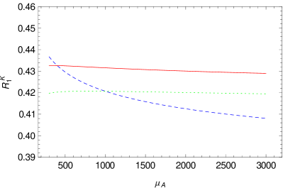
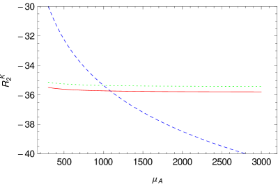
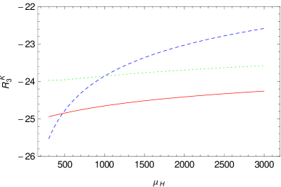
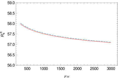
Figure 5: The quantities $R_{i}^{K}$ defined in Eq. (33)–(36) as a function of $\mu_{A,H}$ for $M_{A,H}=1~{}$TeV. In the first row are the results for the gauge boson exchange and in the second row for scalar exchange. The dashed blue line represents the LO calculation for the Wilson coefficients, the dotted green line includes only logarithmic $\mathcal{O}(\alpha_{s})$ corrections which reduces the scale dependence and the solid red line includes both logarithmic and non-logarithmic $\mathcal{O}(\alpha_{s})$ corrections that is important for the cancellation of scale and scheme dependence.

In order to find numerical values of $P_{i}^{a}$ one needs the values of the corresponding non-perturbative parameters $B^{a}_{i}$ defined in [11]. These are given in terms of the parameters $B_{i}$ used in [8, 9, 23, 24] as follows:

$$B_{1}^{\text{VLL}}(\mu_{0})=B_{1}^{\text{VRR}}(\mu_{0})=B_{1}(\mu_{0})\,,$$ (37a)

$$B_{1}^{\text{LR}}(\mu_{0})=B_{5}(\mu_{0})\,,$$ (37b)

$$B_{2}^{\text{LR}}(\mu_{0})=B_{4}(\mu_{0})\,,$$ (37c)

$$B_{1}^{\text{SLL}}(\mu_{0})=B_{2}^{\text{SRR}}(\mu_{0})=B_{2}(\mu_{0})\,,$$ (37d)

$$B_{2}^{\text{SLL}}(\mu_{0})=B_{2}^{\text{SRR}}(\mu_{0})=\frac{5}{3}B_{2}(\mu_{0})-\frac{2}{3}B_{3}(\mu_{0})\,.$$ (37e)

The values for $B_{i}$ in the $\overline{\rm MS}$-NDR scheme extracted from [23] for the $K^{0}-\bar{K}^{0}$ system are collected in Table 1, together with the relevant value of $\mu_{0}$.

	$B_{1}$	$B_{2}$	$B_{3}$	$B_{4}$	$B_{5}$	$\mu_{0}$
$K^{0}$-$\bar{K}^{0}$	0.57	0.68	1.10	0.81	0.56	2.0  GeV

Table 1: Values of the parameters $B_{i}$ in the $\overline{\text{MS}}$-NDR scheme obtained in [23] for $K^{0}-\bar{K}^{0}$ system. The scale $\mu_{0}$ at which $B_{i}$ are evaluated is given in the last column.

In each case we vary conservatively the matching scale between $300\,{\rm GeV}$ and $3000\,{\rm GeV}$ and show in each plot three curves:

• The result without the inclusion of ${\cal O}(\alpha_{s})$ corrections as used until now in the literature (blue, dashed line).

• The result after only logarithmic terms in the ${\cal O}(\alpha_{s})$ have been included. They are crucial for the cancellation of the matching scale dependence (green, dotted line).

• The result after the inclusion of non-logarithmic ${\cal O}(\alpha_{s})$ corrections that are crucial for the cancellation of the renormalization scheme dependence (red, solid line).

These plots are self-explanatory and we make only a few comments:

• As expected the dotted green lines cross the dashed blue lines at $\mu_{A,H}=1000\,{\rm GeV}$.

• The crossing point between the solid red and dashed blue lines is generally at $\mu_{A,H}$ that differs from the mass $M_{A,H}=1000\,{\rm GeV}$ of the exchanged particle. The modest size of these differences shows that these corrections are small, of ${\cal O}(5)\%$ in the NDR-$\overline{\text{MS}}$ scheme.

• In the case of gauge boson exchanges the matching scale dependence of roughly $10(25)\%$ for VLL(LR) operators in the range considered, when ${\cal O}(\alpha_{s})$ corrections are not taken into account, has been reduced down to $1-2\%$ after the inclusion of these corrections.

• In the case of scalar exchanges the matching scale dependence in the case of the SLL sector of roughly $10\%$ in the range considered, when ${\cal O}(\alpha_{s})$ corrections are not taken into account, has been reduced down to $1-2\%$ after the inclusion of ${\cal O}(\alpha_{s})$ corrections.

• In the case of LR operators in the scalar case there is basically no left-over scale dependence even in the LO as we explained at the end of Section 4.

This reduction of scale uncertainties cannot be appreciated at present in view of significant uncertainties in the values of the $B_{i}$ parameters, as seen in Table 1, but the recent advances in lattice calculations allow for optimism and we expect that during this decade these uncertainties could be reduced below $5\%$ and then the calculations presented here will turn out to be important.

7 Summary

If there is a new physics at distance scales as short as $10^{-19}-10^{-21}$ m, it will manifest itself primarily not through penguin and box diagrams as in the SM but through tree level FCNC processes. The best known examples of such NP are various versions of the so-called $Z^{\prime}$ models in which new neutral heavy weak boson ($Z^{\prime}$) mediate FCNC processes already at tree level. Gauged flavour models with new very heavy neutral gauge bosons and Left-Right symmetric models with heavy neutral scalars are other prominent examples where tree-level contributions to $\Delta F=2$ amplitudes are present.

Effective tree-level contributions to $\Delta F=2$ observables can also be generated at one loop in models having GIM at the fundamental level and Minimal Flavour Violation of which Two-Higgs Doublet Models with and without supersymmetry are the best known examples. In models with heavy vectorial fermions that mix with the standard chiral quarks and models in which $Z^{0}$ and SM neutral Higgs $H^{0}$ mix with new heavy gauge bosons and scalars in the process of electroweak symmetry breaking also tree-level contributions to $\Delta F=2$ processes mediated by $Z^{0}$ and SM neutral Higgs $H^{0}$ are possible. In all these extensions new local operators absent in the SM are generated having Wilson coefficients that are generally much stronger affected by renormalization group QCD effects than it is the case of the SM operators.

Present studies of renormalization group QCD effects performed at the NLO level in many extensions of the SM use the so-called $P_{i}^{a}$ QCD factors [11] that include both hadronic matrix elements of contributing operators and renormalization group evolution from high energy to low energy scales. These factors represent the dominant part of any NLO QCD analysis but do not take into account ${\cal O}(\alpha_{s})$ corrections to Wilson coefficients at the matching scale which separates the full and effective theories. Therefore basically all published calculations that considered tree level decays suffer from some unphysical scale and renormalization scheme dependences. While presently these unphysical effects are much smaller than the uncertainties in the hadronic matrix elements of contributing operators, the situation could change in this decade due to important progress in lattice simulations with dynamical fermions [25, 26, 27, 28, 29, 30, 31, 32, 33].

While a general calculations of ${\cal O}(\alpha_{s})$ corrections to Wilson coefficients, when the leading contributions come from loop diagrams, is very model dependent, a rather general analysis can be done for tree level exchanges so that the final results depend only on the couplings of exchanged bosons (vectors and scalars), on the QCD colour factors and the QCD coupling constant.

The main goal of our analysis was to provide analytical formulae for arbitrary number of colours ($N$) for the ${\cal O}(\alpha_{s})$ corrections in question in the case of tree level $\Delta F=2$ processes mediated by heavy colourless gauge bosons and scalars. The results for the Wilson Coefficients and effective Hamiltonians for these cases are collected in Section 3, while the corresponding mixing amplitudes at the NLO level that combine our results with the known $P_{i}^{a}$ QCD factors are presented in Section 5. In Section 6 we demonstrated that the unphysical scale dependences have practically been removed by our calculations. This is particularly important for the LR system in the case of gauge boson exchanges, where the scale dependence at LO is sizeable. The Appendices collect certain technicalities about the evanescent operators and intermediate results in the full and effective theories which should enable interested readers to check our calculations.

Acknowledgements

We would like to thank Gerhard Buchalla, Andreas Kronfeld, Mikolaj Misiak and Ulrich Nierste for discussions. This research was done in the context of the ERC Advanced Grant project “FLAVOUR”(267104) and was partially supported by the DFG cluster of excellence “Origin and Structure of the Universe”.

Appendix A The issue of Evanescent Operators

It is well known that in the process of NLO calculations in the NDR-$\overline{\text{MS}}$ scheme, where ultraviolet divergences are regulated dimensionally, the so-called evanescent operators that vanish in $D=4$ dimensions have to be considered. They arise in particular when complicated Dirac structures are projected onto the chosen basis of physical operators. The treatment of this operators in the process of matching considered by us must be consistent with the one used in the calculation of two-loop anomalous dimensions.

We have used the $P_{i}^{a}$ QCD factors from [11] which were based on the two-loop anomalous dimensions of operators calculated in [10]. Therefore it is mandatory for us to treat evanescent operators appearing in our calculations in the same manner as done in [10]. Now, the latter paper used the treatment of evanescent operators as proposed in the context of the formulation of the NDR-$\overline{\text{MS}}$ scheme introduced in [22]. The virtue of this treatment is that the evanescent operators defined in this scheme influence only two-loop anomalous dimensions. By definition they do not contribute to the matching and to the finite corrections to the matrix elements of renormalized operators calculated by us. They are simply subtracted away in the process of renormalization. This issue is summarized in Section 6.9.4 of [20], where further references can be found. A very important paper in this context is [34]. Therefore effectively the calculations presented here were based on the projections listed in the next appendix that leave out the evanescent operators on the r.h.s.

In this context we should warn the reader that the NDR-$\overline{\text{MS}}$ scheme used in [35], while sharing all the virtues of the scheme of [22] uses different projections in the SLL sector. This implies different two-loop anomalous dimensions for the SLL operators, that is also different $P_{i}^{\rm SLL}$ and also different ${\cal O}(\alpha_{s})$ terms in $C_{i}^{\rm SLL}(\mu_{\rm in})$ so that the physical amplitudes are the same in both schemes. The relation between these two schemes has been worked out in [12].

Another technical issue is related to the Fierz-vanishing evanescent operators, which have to be considered when one wants to relate the operators with non-singlet structures like

$$\tilde{Q}_{1}^{\rm SLL} = (\bar{s}^{\alpha}P_{L}d^{\beta})(\bar{s}^{\beta}P_{L}d^{\alpha}),$$ (38)

$$\tilde{Q}_{2}^{\rm SLL} = (\bar{s}^{\alpha}\sigma_{\mu\nu}P_{L}d^{\beta})(\bar{s}^{\beta}\sigma^{\mu\nu}P_{L}d^{\alpha})$$ (39)

to the operators $Q_{1,2}^{\rm SLL}$ used by us. In $D=4-2\epsilon$ dimensions the usual $D=4$ identities

$$\tilde{Q}_{1}^{\rm SLL}\mathrel{\mathop{\kern 0.0pt=}\limits_{D=4}}-\frac{1}{2}\,Q_{1}^{\rm SLL}+\frac{1}{8}\,Q_{2}^{\rm SLL},$$ (40)

$$\tilde{Q}_{2}^{\rm SLL}\mathrel{\mathop{\kern 0.0pt=}\limits_{D=4}}6\,Q_{1}^{\rm SLL}+\frac{1}{2}\,Q_{2}^{\rm SLL}.$$ (41)

do not work and one has to add evanescent operators on the r.h.s of these equations. However again, even if the inclusion of the latter operators was relevant for the calculation of two-loop anomalous dimensions of the physical operators in [10], it turns out that they do not contribute to the matching as long as the infrared divergences are not regulated dimensionally. As in our paper we regulated such divergences by a non-vanishing $p^{2}$, we can use the relations in Eq. (40) and Eq. (41) without taking the Fierz-vanishing evanescent operators in question into account. As discussed in [10] these “problems” are absent in the case of other operators.

Appendix B Projections

We list projections of all Dirac structures on physical operators that we encountered in our calculations. These projections correspond to the so-called “Greek method” as described in Section 6.9 of [22]. The evanescent operators, relevant in this renormalization scheme only at two-loop level, are defined as the differences of l.h.s and r.h.s of these equations. See [10] for more details. We define $\sigma_{\mu\nu}=\frac{1}{2}\left[\gamma_{\nu},\,\gamma_{\nu}\right]$.

$$\gamma_{\alpha}\gamma_{\beta}\gamma_{\mu}(1\pm\gamma_{5})\gamma^{\beta}\gamma^{\alpha}\otimes\gamma^{\mu}(1\pm\gamma_{5})=4(1-2\epsilon)\,\gamma_{\mu}(1\pm\gamma_{5})\otimes\gamma^{\mu}(1\pm\gamma_{5})$$ (42a)

$$\gamma_{\mu}(1\pm\gamma_{5})\gamma_{\alpha}\gamma_{\beta}\otimes\gamma^{\mu}(1\pm\gamma_{5})\gamma^{\alpha}\gamma^{\beta}=4(4-\epsilon)\,\gamma_{\mu}(1\pm\gamma_{5})\otimes\gamma^{\mu}(1\pm\gamma_{5})$$ (42b)

$$\gamma_{\mu}(1\pm\gamma_{5})\gamma_{\alpha}\gamma_{\beta}\otimes\gamma^{\beta}\gamma^{\alpha}\gamma^{\mu}(1\pm\gamma_{5})=4(1-2\epsilon)\,\gamma_{\mu}(1\pm\gamma_{5})\otimes\gamma^{\mu}(1\pm\gamma_{5})$$ (42c)

$$\gamma_{\alpha}\gamma_{\beta}\gamma_{\mu}(1\pm\gamma_{5})\gamma^{\beta}\gamma^{\alpha}\otimes\gamma^{\mu}(1\mp\gamma_{5})=4(1-2\epsilon)\,\gamma_{\mu}(1\pm\gamma_{5})\otimes\gamma^{\mu}(1\mp\gamma_{5})$$ (43a)

$$\gamma_{\mu}(1\pm\gamma_{5})\gamma_{\alpha}\gamma_{\beta}\otimes\gamma^{\mu}(1\mp\gamma_{5})\gamma^{\alpha}\gamma^{\beta}=4(1+\epsilon)\,\gamma_{\mu}(1\pm\gamma_{5})\otimes\gamma^{\mu}(1\mp\gamma_{5})$$ (43b)

$$\gamma_{\mu}(1\pm\gamma_{5})\gamma_{\alpha}\gamma_{\beta}\otimes\gamma^{\beta}\gamma^{\alpha}\gamma^{\mu}(1\mp\gamma_{5})=\,16(1-\epsilon)\gamma_{\mu}(1\pm\gamma_{5})\otimes\gamma_{\mu}(1\mp\gamma_{5})$$ (43c)

$$\gamma_{\nu}\gamma_{\mu}(1\mp\gamma_{5})\gamma^{\mu}\gamma^{\nu}\otimes(1\pm\gamma_{5})=16(1-\epsilon)\,(1\mp\gamma_{5})\otimes(1\pm\gamma_{5})$$ (44a)

$$(1\mp\gamma_{5})\gamma_{\mu}\gamma_{\nu}\otimes(1\pm\gamma_{5})\gamma^{\mu}\gamma^{\nu}=4(1+\epsilon)\,(1\mp\gamma_{5})\otimes(1\pm\gamma_{5})$$ (44b)

$$(1\mp\gamma_{5})\gamma_{\mu}\gamma_{\nu}\otimes\gamma^{\mu}\gamma^{\nu}(1\pm\gamma_{5})=4(1-2\epsilon)\,(1\mp\gamma_{5})\otimes(1\pm\gamma_{5})$$ (44c)

$$\gamma_{\nu}\gamma_{\mu}(1\pm\gamma_{5})\gamma^{\mu}\gamma^{\nu}\otimes(1\pm\gamma_{5})=16(1-\epsilon)\,(1\pm\gamma_{5})\otimes(1\pm\gamma_{5})$$ (45a)

$$\begin{split}&(1\pm\gamma_{5})\gamma_{\mu}\gamma_{\nu}\otimes(1\pm\gamma_{5})\gamma^{\mu}\gamma^{\nu}\\ &\quad=(4-2\epsilon)\,(1\pm\gamma_{5})\otimes(1\pm\gamma_{5})+\sigma_{\mu\nu}(1\pm\gamma_{5})\otimes\sigma^{\mu\nu}(1\pm\gamma_{5})\end{split}$$ (45b)

$$\begin{split}&(1\pm\gamma_{5})\gamma_{\mu}\gamma_{\nu}\otimes\gamma^{\nu}\gamma^{\mu}(1\pm\gamma_{5})\\ &\quad=(4-2\epsilon)\,(1\pm\gamma_{5})\otimes(1\pm\gamma_{5})-\sigma_{\mu\nu}(1\pm\gamma_{5})\otimes\sigma^{\mu\nu}(1\pm\gamma_{5})\end{split}$$ (45c)

$$\gamma^{\alpha}\gamma^{\beta}\sigma^{\mu\nu}(1\pm\gamma_{5})\gamma_{\beta}\gamma_{\alpha}\otimes\sigma^{\mu\nu}(1\pm\gamma_{5})=0$$ (46a)

$$\begin{split}&\sigma_{\mu\nu}(1\pm\gamma_{5})\gamma_{\alpha}\gamma_{\beta}\otimes\sigma^{\mu\nu}(1\pm\gamma_{5})\gamma^{\alpha}\gamma^{\beta}\\ &\quad=(48-80\epsilon)\,(1\pm\gamma_{5})\otimes(1\pm\gamma_{5})+(12-6\epsilon)\,\sigma_{\mu\nu}(1\pm\gamma_{5})\otimes\sigma^{\mu\nu}(1\pm\gamma_{5})\end{split}$$ (46b)

$$\begin{split}&\sigma_{\mu\nu}(1\pm\gamma_{5})\gamma_{\alpha}\gamma_{\beta}\otimes\gamma^{\beta}\gamma^{\alpha}\sigma^{\mu\nu}(1\pm\gamma_{5})\\ &\quad=-(48-80\epsilon)\,(1\pm\gamma_{5})\otimes(1\pm\gamma_{5})+(12-14\epsilon)\,\sigma_{\mu\nu}(1\pm\gamma_{5})\otimes\sigma^{\mu\nu}(1\pm\gamma_{5})\end{split}$$ (46c)

Appendix C Matrix Elements of Operators

After quark wave function renormalization and operator renormalization we get

$$\langle Q_{1}^{\text{VLL}}\rangle =\left[1+2C_{F}\frac{\alpha_{s}}{4\pi}\log\frac{\mu^{2}}{-p^{2}}-3\frac{N-1}{N}\frac{\alpha_{s}}{4\pi}\left(\log\frac{\mu^{2}}{-p^{2}}+\frac{7}{3}\right)\right]Q_{1}^{\text{VLL}}$$ (47)

$$\begin{split}\langle Q_{1}^{\text{LR}}\rangle&=\left[1+2C_{F}\frac{\alpha_{s}}{4\pi}\log\frac{\mu^{2}}{-p^{2}}\right]Q_{1}^{\text{LR}}-6\frac{\alpha_{s}}{4\pi}\left(\log\frac{\mu^{2}}{-p^{2}}+\frac{1}{3}\right)\left(\frac{1}{2N}Q_{1}^{\text{LR}}+Q_{2}^{\text{LR}}\right)\end{split}$$ (48)

$$\begin{split}\langle Q_{2}^{\text{LR}}\rangle&=\left[1+8C_{F}\frac{\alpha_{s}}{4\pi}\left(1+\log\frac{\mu^{2}}{-p^{2}}\right)\right]Q_{2}^{\text{LR}}+6\frac{\alpha_{s}}{4\pi}\left(\frac{1}{2N}Q_{2}^{\text{LR}}+\frac{1}{4}Q_{1}^{\text{LR}}\right)\end{split}$$ (49)

$$\begin{split}\langle Q_{1}^{\text{SLL}}\rangle&=\left[1+8C_{F}\frac{\alpha_{s}}{4\pi}\left(1+\log\frac{\mu^{2}}{-p^{2}}\right)\right]Q_{1}^{\text{SLL}}\\ &\quad-\frac{\alpha_{s}}{4\pi}\left(2+\log\frac{\mu^{2}}{-p^{2}}\right)\left(\frac{N-2}{4N}Q_{2}^{\text{SLL}}+3Q_{1}^{\text{SLL}}\right)\end{split}$$ (50)

$$\begin{split}\langle Q_{2}^{\text{SLL}}\rangle&=Q_{2}^{\text{SLL}}-48\frac{\alpha_{s}}{4\pi}\left(\log\frac{\mu^{2}}{-p^{2}}+\frac{1}{3}\right)\left(-\frac{N+2}{4N}Q_{1}^{\text{SLL}}+\frac{1}{16}Q_{2}^{\text{SLL}}\right)\\ &\quad-4\frac{\alpha_{s}}{4\pi}\left(\frac{N-2}{4N}Q_{2}^{\text{SLL}}+3Q_{1}^{\text{SLL}}\right)\end{split}$$ (51)

We remark that for the matching performed in this paper only the ${\cal O}(\alpha_{s})$ corrections to the matrix elements $\langle Q_{1}^{\text{VLL}}\rangle$, $\langle Q_{1}^{\text{LR}}\rangle$ and $\langle Q_{1}^{\text{SLL}}\rangle$ matter. We give the remaining matrix elements as they are relevant for NLO matching when coloured gauge bosons and scalars are exchanged [19].

Appendix D Amplitudes in the Full Theory

Colourless gauge boson exchange (after quark wave function renormalization):

$$(\mathcal{A}^{\text{VLL}}_{1})^{\text{gauge}}= \frac{(\Delta_{L}^{sd}(A))^{2}}{2M_{A}^{2}}\left[1+2C_{F}\frac{\alpha_{s}}{4\pi}\log\frac{\mu^{2}}{-p^{2}}-3\frac{N-1}{N}\frac{\alpha_{s}}{4\pi}\left(\frac{1}{2}+\log\frac{M^{2}_{A}}{-p^{2}}\right)\right]Q_{1}^{\text{VLL}}$$ (52)

$$\begin{split}(\mathcal{A}^{\text{LR}}_{1})^{\text{gauge}}=&\frac{\Delta_{L}^{sd}(A)\Delta_{R}^{sd}(A)}{M_{A}^{2}}\left[\left(1+2C_{F}\frac{\alpha_{s}}{4\pi}\log\frac{\mu^{2}}{-p^{2}}\right)Q_{1}^{\text{LR}}\right.\\ &\qquad\qquad\qquad\quad\left.-\frac{\alpha_{s}}{4\pi}\left(\frac{1}{2}+\log\frac{M^{2}_{A}}{-p^{2}}\right)\left(\frac{3}{N}Q_{1}^{\text{LR}}+6Q_{2}^{\text{LR}}\right)\right]\end{split}$$ (53)

Colourless scalar exchange (after quark wave function and quark mass renormalization):

$$(\mathcal{A}^{\text{LR}}_{2})^{\text{scalar}}= -\frac{\Delta_{L}^{sd}(H)\Delta_{R}^{sd}(H)}{M_{H}^{2}}\left[1+8C_{F}\frac{\alpha_{s}}{4\pi}\left(1+\log\frac{\mu^{2}}{-p^{2}}\right)\right]Q_{2}^{\text{LR}}$$ (54)

$$\begin{split}(\mathcal{A}^{\text{SLL}}_{1})^{\text{scalar}}=&-\frac{(\Delta_{L}^{sd}(H))^{2}}{2M_{H}^{2}}\left[\left(1+8C_{F}\frac{\alpha_{s}}{4\pi}\left(1+\log\frac{\mu^{2}}{-p^{2}}\right)\right)Q_{1}^{\text{SLL}}\right.\\ &\qquad\qquad\qquad\quad\left.-\frac{\alpha_{s}}{4\pi}\left(\frac{1}{2}+\log\frac{M^{2}_{H}}{-p^{2}}\right)\left(\frac{N-2}{4N}Q_{2}^{\text{SLL}}+3Q_{1}^{\text{SLL}}\right)\right]\end{split}$$ (55)

References

• [1] S. L. Glashow, J. Iliopoulos, and L. Maiani, Weak interactions with lepton-hadron symmetry, Phys. Rev. D 2 (Oct, 1970) 1285–1292.
• [2] P. Langacker, The Physics of Heavy $Z^{\prime}$ Gauge Bosons, Rev.Mod.Phys. 81 (2009) 1199–1228, [arXiv:0801.1345].
• [3] B. Grinstein, M. Redi, and G. Villadoro, Low Scale Flavor Gauge Symmetries, JHEP 1011 (2010) 067, [arXiv:1009.2049].
• [4] UTfit Collaboration Collaboration, M. Bona et. al., Model-independent constraints on $\Delta$ F=2 operators and the scale of new physics, JHEP 0803 (2008) 049, [arXiv:0707.0636].
• [5] M. Antonelli, D. M. Asner, D. A. Bauer, T. G. Becher, M. Beneke, et. al., Flavor Physics in the Quark Sector, Phys.Rept. 494 (2010) 197–414, [arXiv:0907.5386].
• [6] G. Isidori, Y. Nir, and G. Perez, Flavor Physics Constraints for Physics Beyond the Standard Model, Ann.Rev.Nucl.Part.Sci. 60 (2010) 355, [arXiv:1002.0900].
• [7] J. A. Bagger, K. T. Matchev, and R.-J. Zhang, QCD corrections to flavor changing neutral currents in the supersymmetric standard model, Phys.Lett. B412 (1997) 77–85, [hep-ph/9707225].
• [8] M. Ciuchini, E. Franco, V. Lubicz, G. Martinelli, I. Scimemi, et. al., Next-to-leading order QCD corrections to $\Delta F=2$ effective Hamiltonians, Nucl.Phys. B523 (1998) 501–525, [hep-ph/9711402].
• [9] M. Ciuchini, V. Lubicz, L. Conti, A. Vladikas, A. Donini, et. al., $\Delta M_{K}$ and $\epsilon_{K}$ in SUSY at the next-to-leading order, JHEP 9810 (1998) 008, [hep-ph/9808328]. Erratum added online, Mar/29/2000.
• [10] A. J. Buras, M. Misiak, and J. Urban, Two loop QCD anomalous dimensions of flavor changing four quark operators within and beyond the standard model, Nucl.Phys. B586 (2000) 397–426, [hep-ph/0005183].
• [11] A. J. Buras, S. Jager, and J. Urban, Master formulae for $\Delta F=2$ NLO QCD factors in the standard model and beyond, Nucl.Phys. B605 (2001) 600–624, [hep-ph/0102316].
• [12] M. Gorbahn, S. Jager, U. Nierste, and S. Trine, The supersymmetric Higgs sector and $B-\bar{B}$ mixing for large $\tan\beta$, Phys.Rev. D84 (2011) 034030, [arXiv:0901.2065].
• [13] A. J. Buras, M. V. Carlucci, S. Gori, and G. Isidori, Higgs-mediated FCNCs: Natural Flavour Conservation vs. Minimal Flavour Violation, JHEP 1010 (2010) 009, [arXiv:1005.5310].
• [14] A. J. Buras, G. Isidori, and P. Paradisi, EDMs versus CPV in $B_{s,d}$ mixing in two Higgs doublet models with MFV, Phys.Lett. B694 (2011) 402–409, [arXiv:1007.5291].
• [15] A. J. Buras, K. Gemmler, and G. Isidori, Quark flavour mixing with right-handed currents: an effective theory approach, Nucl.Phys. B843 (2011) 107–142, [arXiv:1007.1993].
• [16] M. Blanke, A. J. Buras, K. Gemmler, and T. Heidsieck, $\Delta F=2$ observables and $B\to X_{q}\gamma$; in the Left-Right Asymmetric Model: Higgs particles striking back, arXiv:1111.5014.
• [17] A. J. Buras, M. V. Carlucci, L. Merlo, and E. Stamou, Phenomenology of a Gauged $SU(3)^{3}$ Flavour Model, arXiv:1112.4477.
• [18] A. J. Buras, Climbing NLO and NNLO Summits of Weak Decays, arXiv:1102.5650.
• [19] A. J. Buras and J. Girrbach, “Complete NLO QCD Corrections for Tree Level $\Delta F=2$ FCNC Processes: Coloured Gauge Bosons and Scalars.” , in preparation.
• [20] A. J. Buras, Weak Hamiltonian, CP violation and rare decays, hep-ph/9806471. To appear in ’Probing the Standard Model of Particle Interactions’, F.David and R. Gupta, eds., 1998, Elsevier Science B.V.
• [21] A. J. Buras, M. Jamin, and P. H. Weisz, Leading and next-to-leading QCD corrections to $\varepsilon$ parameter and $B^{0}-\bar{B}^{0}$ mixing in the presence of a heavy top quark, Nucl. Phys. B347 (1990) 491–536.
• [22] A. J. Buras and P. H. Weisz, QCD Nonleading Corrections to Weak Decays in Dimensional Regularization and ’t Hooft-Veltman Schemes, Nucl.Phys. B333 (1990) 66.
• [23] R. Babich et. al., $K^{0}-\bar{K}^{0}$ mixing beyond the standard model and CP-violating electroweak penguins in quenched QCD with exact chiral symmetry, Phys. Rev. D74 (2006) 073009, [hep-lat/0605016].
• [24] D. Becirevic, V. Gimenez, G. Martinelli, M. Papinutto, and J. Reyes, B-parameters of the complete set of matrix elements of $\Delta B=2$ operators from the lattice, JHEP 04 (2002) 025, [hep-lat/0110091].
• [25] RBC Collaboration, D. J. Antonio et. al., Neutral kaon mixing from 2+1 flavor domain wall QCD, Phys. Rev. Lett. 100 (2008) 032001, [hep-ph/0702042].
• [26] C. Aubin, J. Laiho, and R. S. Van de Water, The Neutral kaon mixing parameter B(K) from unquenched mixed-action lattice QCD, Phys.Rev. D81 (2010) 014507, [arXiv:0905.3947].
• [27] J. Laiho, E. Lunghi, and R. S. Van de Water, Lattice QCD inputs to the CKM unitarity triangle analysis, Phys. Rev. D81 (2010) 034503, [arXiv:0910.2928]. Updates available on http://latticeaverages.org/.
• [28] T. Bae, Y.-C. Jang, C. Jung, H.-J. Kim, J. Kim, et. al., $B_{K}$ using HYP-smeared staggered fermions in $N_{f}=2+1$ unquenched QCD, Phys.Rev. D82 (2010) 114509, [arXiv:1008.5179].
• [29] ETM Collaboration Collaboration, M. Constantinou et. al., $B_{K}$-parameter from $N_{f}$ = 2 twisted mass lattice QCD, Phys.Rev. D83 (2011) 014505, [arXiv:1009.5606].
• [30] Y. Aoki, R. Arthur, T. Blum, P. Boyle, D. Brommel, et. al., Continuum Limit of $B_{K}$ from 2+1 Flavor Domain Wall QCD, Phys.Rev. D84 (2011) 014503, [arXiv:1012.4178].
• [31] C. McNeile, C. Davies, E. Follana, K. Hornbostel, and G. Lepage, High-Precision $f_{B_{s}}$ and HQET from Relativistic Lattice QCD, arXiv:1110.4510.
• [32] C. Bouchard, E. Freeland, C. Bernard, A. El-Khadra, E. Gamiz, et. al., Neutral $B$ mixing from $2+1$ flavor lattice-QCD: the Standard Model and beyond, arXiv:1112.5642.
• [33] for the Fermilab Lattice Collaboration, for the MILC Collaboration Collaboration, E. Neil et. al., B and D meson decay constants from 2+1 flavor improved staggered simulations, arXiv:1112.3978.
• [34] S. Herrlich and U. Nierste, Evanescent operators, scheme dependences and double insertions, Nucl.Phys. B455 (1995) 39–58, [hep-ph/9412375].
• [35] M. Beneke, G. Buchalla, C. Greub, A. Lenz, and U. Nierste, Next-to-leading order QCD corrections to the lifetime difference of $B_{s}$ mesons, Phys.Lett. B459 (1999) 631–640, [hep-ph/9808385].