Towards the production of ultracold ground-state RbCs molecules:
Feshbach resonances, weakly bound states, and coupled-channel model

Abstract

We have studied interspecies scattering in an ultracold mixture of ⁸⁷Rb and ¹³³Cs atoms, both in their lowest-energy spin states. The three-body loss signatures of 30 incoming $s$- and $p$-wave magnetic Feshbach resonances over the range 0 to 667 G have been catalogued. Magnetic field modulation spectroscopy was used to observe molecular states bound by up to 2.5 MHz$\times h$. We have created RbCs Feshbach molecules using two of the resonances. Magnetic moment spectroscopy along the magneto-association pathway from 197 to 182 G gives results consistent with the observed and calculated dependence of the binding energy on magnetic field strength. We have set up a coupled-channel model of the interaction and have used direct least-squares fitting to refine its parameters to fit the experimental results from the Feshbach molecules, in addition to the Feshbach resonance positions and the spectroscopic results for deeply bound levels. The final model gives a good description of all the experimental results and predicts a large resonance near 790 G, which may be useful for tuning the interspecies scattering properties. Quantum numbers and vibrational wavefunctions from the model can also be used to choose optimal initial states of Feshbach molecules for their transfer to the rovibronic ground state using stimulated Raman adiabatic passage (STIRAP).

I Introduction

Dilute quantum gases are ideal for studying many-body physics, because they provide model systems in which the parameters can be precisely controlled. External fields can be used to tune the effective isotropic contact interactions between the particles, and the geometry and strength of the confining optical potentials can be controlled by laser beams. For example, quantum-gas analogues of superconductivity Zwierlein et al. (2005) and the superfluid-to-Mott-insulator quantum phase transition Greiner et al. (2002) have been observed in the laboratory, and their properties have been shown to agree beautifully with the predictions from theoretical models Giorgini et al. (2008). Recently, quantum gases of particles with long-range anisotropic interactions have been created Griesmaier et al. (2005, 2006); Ni et al. (2008). For particles with permanent electric dipole moments, the range of the dipole-dipole interactions can be much larger than typical optical lattice spacings, and interesting new quantum phases and quantum information applications have been proposed Góral et al. (2002); Büchler et al. (2007); Micheli et al. (2007); Pupillo et al. (2008); Wall and Carr (2009). A quantum gas of ⁴⁰K⁸⁷Rb ground-state molecules is the only such system that presently exists in the laboratory Ni et al. (2008).

Our goal is to generate a dipolar quantum gas of ground-state ⁸⁷Rb¹³³Cs, which, unlike KRb, is expected to be collisionally stable because both the exchange reaction 2RbCs $\rightarrow$ Rb₂ + Cs₂ and trimer formation reactions are endothermic Żuchowski and Hutson (2010). Although other approaches are under development Bethlem and Meijer (2003); Sage et al. (2005); Deiglmayr et al. (2008); Aikawa et al. (2010), the only method currently available to produce high phase-space density gases of ground-state molecules is to create weakly bound molecules from ultracold atomic gases by magnetic tuning across a Feshbach resonance Regal et al. (2003); Herbig et al. (2003), and then to transfer the molecules to the rovibronic ground state by stimulated Raman adiabatic passage (STIRAP) Bergmann et al. (1998); Winkler et al. (2007); Danzl et al. (2008); Ni et al. (2008); Lang et al. (2008); Mark et al. (2009); Danzl et al. (2010). As a first step, we have performed evaporative cooling on Rb and Cs samples in separate optical traps, combining them at the end to obtain an Rb-Cs mixture with high phase-space density Lercher et al. (2011). We have successfully used this mixture to produce ultracold samples of weakly bound RbCs Debatin et al. (2011). In this paper, we present a combined experimental and theoretical study of the interspecies Feshbach resonances and weakly bound molecular energy levels of Rb-Cs and use the results to develop an accurate coupled-channel model of the interaction, based on the derived interaction potentials for the molecular states $X\,^{1}\Sigma^{+}$ and $a\,^{3}\Sigma^{+}$.

II Overview

The work described in this paper involved a close collaboration between experiment and theory. At the start of the work, the Feshbach resonances and bound states observed experimentally Pilch et al. (2009) were unassigned. In initial theoretical work, we developed preliminary coupled-channel models of the bound states and scattering and used these to propose assignments of quantum numbers to observed energy levels and Feshbach resonances. Experiments were then carried out to test the assignments and extend the early measurements. The whole process was repeated several times. However, to aid understanding, we will describe the experiments in Section III below using quantum numbers based on our final understanding from theory (Section IV), even though the quantum numbers were not known at the outset.

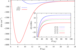
Figure 1: [Color online.] Molecular potential energy curves $V_{0}(R)$ and $V_{1}(R)$ for the singlet and triplet states of RbCs correlating with two separated ${}^{2}S_{1/2}$ ground-state atoms. The inset shows an expanded view of the long-range potentials separating to the four different hyperfine thresholds at zero field, labelled by $(f_{{}^{87}{\rm Rb}},f_{{}^{133}{\rm Cs}})$, but no longer by singlet or triplet.

Two alkali-metal atoms in ${}^{2}S$ states interact at short range to form singlet ($X\,^{1}\Sigma^{+}$) and triplet ($a\,^{3}\Sigma^{+}$) states. Docenko et al. Docenko et al. (2011) have carried out an extensive spectroscopic study of these states by Fourier transform spectroscopy and have developed potential energy curves as shown in Fig. 1. They were able to observe the vibrational ladder up to high-lying levels with outer turning points around 1.5 nm, at which point the coupling between singlet and triplet molecular states is already significant. They also identified in the observed spectra accidental coincidences of singlet and triplet levels deeper within the potential wells, which fixed their relative energy position very well. In the present work, we initially constrained the short-range part of the potential to follow these curves and adjusted the long-range parameters to reproduce the Feshbach resonances and weakly bound states.

The bound states (Feshbach molecules) that are of most interest in the present paper have binding energies of at most a few MHz$\times h$ and require a quite different description. For a heteronuclear bialkali molecule, there are 4 field-free atomic thresholds, which for ⁸⁷Rb¹³³Cs may be labelled in increasing order of energy by $(f_{\rm Rb},f_{\rm Cs})$ = (1,3), (2,3), (1,4), and (2,4), as shown in the inset of Fig. 1. In a magnetic field, each threshold splits into $(2f_{\rm Rb}+1)(2f_{\rm Cs}+1)$ sublevels labelled $|f_{\rm Rb},m_{\rm Rb}\rangle+|f_{\rm Cs},m_{\rm Cs}\rangle$. The Feshbach molecules might be described using two different sets of quantum numbers, either $(f_{\rm Rb},m_{\rm Rb},f_{\rm Cs},m_{\rm Cs})$ or $(f_{\rm Rb},f_{\rm Cs},F,M_{F})$, where $F$ is the resultant of $f_{\rm Rb}$ and $f_{\rm Cs}$ and $M_{F}=m_{\rm Rb}+m_{\rm Cs}$. In the non-rotating case $F$ and $M_{F}$ are exact quantum numbers if there is no external field, but if there is an external magnetic field, it mixes states with different $F$ values, destroying the exactness of $F$ as a quantum number; the character of the Feshbach molecules at the magnetic fields considered here is more accurately described by $(f_{\rm Rb},m_{\rm Rb},f_{\rm Cs},m_{\rm Cs})$. For high magnetic fields, $f_{\rm Rb}$ and $f_{\rm Cs}$ are also no longer good quantum numbers.

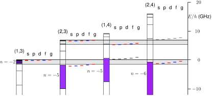
Figure 2: [Color online.] Thresholds for ⁸⁷Rb¹³³Cs and the “bins” (vertical boxes) below each threshold within which each vibrational state must lie for any value of the scattering length. The horizontal boxes, 1.5 GHz deep, show the energy range within which bound levels can cause resonances at the $|1,1\rangle+|3,3\rangle$ and $|2,-1\rangle+|3,3\rangle$ thresholds at fields under 500 G. The vibrational “bin” for each hyperfine state that contains bound states that can cause resonances at the lowest threshold is colored. Selected levels are shown (short horizontal lines) as a function of $L$ ($s$, $p$, $d$, $f$, $g$ for $L=0$, 1, 2, 3, 4) for the specific choice of scattering length that gives a least-bound state for $L=0$ with 110(20) kHz below threshold. For fields below 500 G, only levels $|n(f_{\rm Rb},f_{\rm Cs})\rangle=|{-2}(1,3)\rangle$ and $|{-6}(2,4)\rangle$ can cause resonances at the $|1,1\rangle+|3,3\rangle$ threshold and only levels $|{-4}(1,4)\rangle$ and $|{-2}(2,3)\rangle$ can cause resonances at the $|2,-1\rangle+|3,3\rangle$ threshold.

Additional quantum numbers are needed for the molecules’ end-over-end angular momentum $L$ and the molecular vibration. For near-dissociation levels it is convenient to specify the vibrational quantum number with respect to the asymptote of the atom pair, so that the topmost level is $n=-1$, the next is $n=-2$, and so on. Each level lies within a “bin” below its associated dissociation threshold, with the boundaries of the bins determined by the long-range forces between the atoms. For RbCs, using the published values of the long-range dispersion coefficients, Derevianko et al. (2001); Porsev and Derevianko (2003), which are the same for the singlet and triplet potentials, we find that the $n=-1$ level lies between zero and $-165$ MHz, and the $n=-2$ level lies between $-165$ and $-1150$ MHz. Subsequent lower bin boundaries lie at 3.7, 8.6, 16.7 and 28.8 GHz below threshold for $n=-3$ to $-6$, respectively. As shown below, the actual levels for ⁸⁷RbCs lie close to the top of their bins.

Feshbach resonances occur at fields where a bound state exists at the same energy as the colliding atoms. Zero-energy Feshbach resonances are caused by molecular levels that cross atomic thresholds as a function of magnetic field. Since the level shifts due to the Zeeman effect at fields below 500 G are not more than 1.5 GHz, there is only one vibrational level below each field-free threshold that can cause Feshbach resonances at the $|1,1\rangle+|3,3\rangle$ threshold, as shown in Fig. 2; these are $n=-5$, $-5$ and $-6$ for levels associated with $(f_{\rm Rb},f_{\rm Cs})=(2,3)$, (1,4) and (2,4), respectively. In addition to this, levels very close to dissociation ($n=-1$ or $-2$) corresponding to the same zero-field threshold as the incoming wave can also cause low-field resonances. Fig. 2 also shows the situation at the $|2,-1\rangle+|3,3\rangle$ threshold, which will be considered in Section IV.7.2.

In the general case we label weakly bound states with a complete set of quantum numbers $|n(f_{\rm Rb},f_{\rm Cs})L(m_{\rm Rb},m_{\rm Cs}),M\rangle$, with $L=0,1,2$, etc. designated by $s$, $p$, $d$, etc. $M$ is the sum of all angular momenta projected onto the field axis, $M=m_{\rm Rb}+m_{\rm Cs}+M_{L}$, and is the only exactly conserved quantum number in an external field. Since, however, $M$ is always 4 for the levels studied in this paper (except in sections IV.7.1 and IV.7.2), we will omit it in the following discussion. All other angular momenta are approximate quantum numbers, but are sufficient for proper labeling. We characterize by $L_{\text{c}}=0,1,...$ the partial wave character of the continuum scattering process and speak of incoming $s$- and $p$-wave resonances for $L_{\text{c}}=0$ and $L_{\text{c}}=1$, respectively.

III The Experiments

III.1 Feshbach resonances

Magnetic Feshbach resonances are an important tool for the production of weakly bound molecules and for tuning the scattering length, which determines the elastic and inelastic scattering properties of cold atomic gases Chin et al. (2010). In addition, their positions provide important clues to the molecular bound state structure that lies below the scattering threshold. In previous work Pilch et al. (2009) we observed 23 resonances over the range 0 to 300 G, using a mixture of the lowest spin states, ⁸⁷Rb$|1,1\rangle$ and ¹³³Cs$|3,3\rangle$. Since this mixture was prepared by evaporating both species simultaneously in the same optical trap, interspecies three-body recombination loss and heating Chin et al. (2010) limited the evaporative cooling efficiency, resulting in comparatively high temperatures of 7 $\mu$K and low particle densities of about $5\times 10^{11}$ cm^-3 for each species.

In the current experiment, the mixture is created by combining separately cooled atomic clouds Lercher et al. (2011), so it is much colder (100 to 200 nK) and denser ($5\times 10^{12}$ cm^-3) and gives a much better signal-to-noise ratio for the loss features discussed below. We stop the evaporation procedure before the onset of condensation, because we have previously found the two Bose-Einstein condensates (BECs) to be immiscible Lercher et al. (2011). We hold the mixture at constant magnetic field $B$ for 200 ms. Enhanced losses that occur simultaneously for Rb and Cs are attributed to three-body recombination Chin et al. (2010) at an interspecies Feshbach resonance. We associate the field value $B$ at which maximum atom loss occurs with the pole of the resonance. For example, Fig. 3 shows the atom loss in the vicinity of the resonance near $197$ G.

For sufficiently wide resonances, we find that the number of Rb atoms exhibits a maximum at fields just above resonance. Rb has a lower trap depth than Cs and thus bears most of the heat load through evaporation when the two species are in thermal equilibrium Lercher et al. (2011). Reduced thermalization with Cs at zero interspecies scattering length reduces the heat load on the Rb part of the sample and thus leads to less loss of Rb atoms. This simple explanation allows us to provide an estimate for the resonance width $\Delta$: It is the difference between the field values for the minima (for Rb and Cs) and the maximum (for Rb) as indicated in Fig. 3. A detailed comparison with calculated widths requires a thorough analysis, including three-body and evaporation effects, and will be made in a future publication.

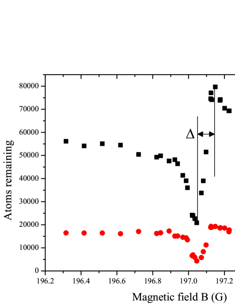
Figure 3: [Color online.] Example of a Feshbach resonance scan showing simultaneous loss for Rb and Cs near 197.06(5) G for a hold time of $200$ ms. The maximum for the number of Rb atoms to the right of the resonance is attributed to the zero crossing for the interspecies scattering length. The difference in the positions of the minima and the maximum as indicated gives an estimate for the resonance width $\Delta$.

As part of this work, we have scanned over a wider range (0 to 667 G) than in Ref. Pilch et al. (2009), finding 7 new incoming $s$-wave resonances in addition to those reported in Ref. Pilch et al. (2009). The old and new resonances are collected together in Table 1. The resonances observed for temperatures $\leq 200$ nK are assigned as incoming $s$-wave ($L_{\text{c}}\!=\!0$) resonances, while those observed at 7 $\mu$K and not observed at 200 nK are assigned as incoming $p$-wave ($L_{\text{c}}\!=\!1$) resonances. The magnetic field is calibrated near each resonance using Rb microwave transitions. The calibration in our previous work Pilch et al. (2009) was based on low-field data and was found to deviate from the current calibration by as much as 0.5 G when extrapolated to 300 G. The positions of the incoming $p$-wave resonances have therefore been scaled to the new calibration, using the incoming $s$-wave resonances observed in both experiments as a reference. The incoming $p$-wave resonances from 258 to 272 G have been remeasured at $4\ \mu$K with the new calibration.

Table 1: ⁸⁷Rb$|1,1\rangle$ + Cs$|3,3\rangle$ Feshbach resonances observed over the range 0–667 G for $s$-wave scattering and 0–300 G for $p$-wave scattering. The magnetic field uncertainties result from a quadrature of resonance position uncertainty due to atom number noise, and an estimated field calibration error of 0.03 G. Resonances too narrow to allow a clear width measurement have no width indicated.

$s$-wave		$p$-wave
Field $B$ (G)	Width $\Delta$ (G)	Field $B$ (G)
181.64(8)	0.27(10)	128.00(25)∗
197.06(5)	0.09(1)	129.60(25)∗
217.34(5)	0.06(1)	140.00(25)∗
225.43(3)	0.16(1)	140.50(25)∗
242.29(5)		234.35(25)∗
247.32(5)	0.09(3)	235.96(25)∗
272.80(4)		258.10(11)
273.45(4)		259.60(11)
273.76(4)		264.19(11)
279.12(5)	0.09(3)	266.23(11)
286.76(5)		271.73(11)
308.44(5)		289.97(25)∗
310.69(6)	0.60(4)	292.08(25)∗
314.74(11)	0.18(10)
352.65(34)	2.70(47)
381.34(5)
421.93(5)

^∗From Ref. Pilch et al. (2009) with field rescaled to current calibration.

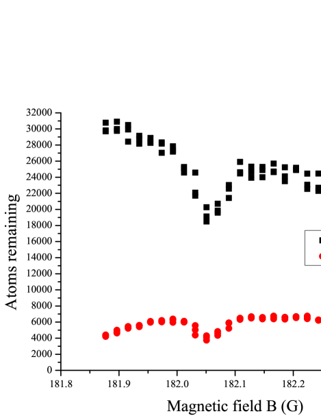
Figure 4: [Color online.] Measurement of the binding energy of the Feshbach molecules. This is an example of a field modulation free-bound resonance scan showing simultaneous loss for Rb and Cs for a hold time of $900$ ms. The modulation frequency is held fixed at $f_{\text{m}}=330$ kHz.

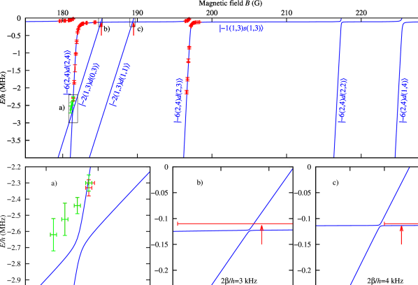
Figure 5: [Color online.] Weakly bound states of RbCs obtained by free-bound (red) and bound-free (green) magnetic-field modulation spectroscopy, together with levels calculated for the final, fitted potentials (blue solid lines). All levels are shown relative to dissociation limit Rb $|1,1\rangle$ + Cs $|3,3\rangle$ at the given magnetic field value $B$. Avoided crossings between the least-bound state and the ramping $n=-2$ levels are shown as red arrows. The smaller panels below, labeled a), b), and c) refer to the areas on the larger panel marked by rectangles and the same labels. The quantity $2\beta$ is the minimum separation in energy between the two states.

III.2 Magnetic-field modulation spectroscopy

We have used magnetic-field modulation spectroscopy Regal et al. (2003); Thompson et al. (2005); Weber et al. (2008); Lange et al. (2009) on our atom mixture to measure binding energies of Feshbach molecules. A set of auxiliary coils modulates the magnetic field $B$ along the quantization axis by up to 0.2 G. Atom losses occur when the modulation frequency $f_{\text{m}}$ is resonant with a free-bound transition (Fig. 4). We observe the losses by holding $f_{\text{m}}$ fixed and scanning $B$, or by holding $B$ fixed and scanning $f_{\text{m}}$. We find that the free-bound signal dies off for $f_{\text{m}}$ above 2.5 MHz and attribute this to lower field amplitudes generated by the coils due to their increased impedance at high frequencies and to the Bessel-function-squared dependence of the coupling strength on the binding energy Beaufils et al. (2010).

The binding energies obtained in this way near the Feshbach resonances at 181.6 G and 197 G are plotted in Fig. 5. Two avoided crossings close below threshold can clearly be identified. We attribute these to the presence of a bound state running parallel to the atomic threshold (with the same magnetic moment as the atom pair) with a binding energy of approximately $110\pm 20$ kHz$\times h$. This “least-bound state” $|n(f_{\rm Rb}f_{\rm Cs})L(m_{\rm Rb}m_{\rm Cs})\rangle=|{-1}(1,3)s(1,3)\rangle$ cannot be observed directly with the modulation technique except near avoided crossings, because the initial and final states involved are exactly equal in all spin quantum numbers; they thus do not differ in magnetic moment and magnetic dipole transitions between them are forbidden. The least-bound state causes avoided crossings directly below the Feshbach resonances by the same coupling mechanism as the Feshbach resonances, and the resulting mixed states can be observed near these crossings. The binding energy of the least-bound state allows us to estimate the interspecies background scattering length as $+645(60)\ a_{0}$ for this scattering channel. This value is further refined in Section IV.6 below. The large value for the scattering length is responsible for the large background interspecies thermalization and three-body loss rates observed previously Lercher et al. (2011); Cho et al. (2011); McCarron et al. (2011).

III.3 Feshbach molecules

To create Feshbach molecules, we sweep the magnetic field $B$ adiabatically from high to low field across one of the Feshbach resonances. The weakly bound molecules formed in this way can collide with atoms and decay to deeply bound states. We must therefore remove the atoms quickly. In previous experiments it was found that the atoms can be removed from the molecular cloud with radiation pressure from a laser (see e.g. Refs. Takekoshi et al. (1998); Xu et al. (2003); Thalhammer et al. (2006)). Here, however, we find that the difference in magnetic moments between the atoms and molecules can be made large enough that the Stern-Gerlach effect due to the magnetic levitation gradient can be used to separate atoms and molecules, allowing us to produce pure samples of 2000 to 4000 RbCs molecules starting from approximately 150000 Rb and 60000 Cs atoms Lercher et al. (2011). The temperature of the molecular cloud is approximately the same as that of the atomic sample, i.e. $100$ to $200$ nK.

We magnetoassociate at either the 197.06 or the 225.43 G resonance, entering the bound-state manifold as seen in Fig. 5. Below each of these Feshbach resonances, there is a strongly avoided crossing with the least-bound state, which we cannot jump over with our finite magnetic switching capability. As a result, immediately after magnetoassociation, the molecules transfer into the least-bound state $|{-1}(1,3)s(1,3)\rangle$, which has a magnetic moment $\mu=-1.3\mu_{\rm B}$, almost identical to that of the free atom pair. In order to separate the atomic and molecular clouds, we switch off the crossed optical dipole force trap confining the atom/molecule mixture and quickly (in 0.5 ms) sweep $B$ down to the next avoided crossing, below the 181.64 or 217.34 G resonance, respectively.

In the case of magnetoassociation at 197.06 G, we cross over onto the low-field-seeking state $|{-6}(2,4)d(2,4)\rangle$ (with $\mu\!=\!+2.0\mu_{\rm B}$) near 182 G, and then use another avoided crossing (Fig. 5, panel (a)) to transfer to the high-field-seeking state $|{-2}(1,3)d(0,3)\rangle$ (with $\mu=-0.9\mu_{\rm B}$). Just before we take the first of these two crossovers, the magnetic field gradient is ramped up to a value suitable for levitating the $|{-2}(1,3)d(0,3)\rangle$ molecules. At this moment, the molecules are still in the least-bound state $|{-1}(1,3)s(1,3)\rangle$ and are pushed upwards together with the atoms. Rb $|1,1\rangle$ and Cs $|3,3\rangle$ have nearly the same magnetic-moment-to-mass ratio at these field values and thus move together. A large downward impulse is imparted to the molecules as they pass through the low-field-seeking state. This separates the atomic cloud from the molecular cloud. After going through the second crossover, the molecules become high-field seekers that are levitated exactly against gravity, and the optical dipole force trap is turned on again, trapping the molecules. The Stern-Gerlach separation takes 3 ms and produces a pure sample of up to 4000 molecules. These are observed by a dissociation ramp backwards along the previous path, after which the Rb and Cs atom clouds are imaged separately.

In the case of magnetoassociation at 225.43 G, we cross over near 217 G onto the $|{-6}(2,4)d(2,2)\rangle$ state, which is also strongly low-field-seeking. To levitate the molecules in this state, the direction of the current in the gradient coils must be switched, causing a delay that results in additional atom-molecule collisions. In this case, we produce pure clouds of typically 2000 molecules.

We note that the molecule creation efficiency of less than $10\%$ is much lower than can be reached under optimized conditions for single-species experiments, e.g. more than $25\%$ or even $30\%$ Mark et al. (2007); Knoop et al. (2008); Mark et al. (2005) for the creation of Feshbach molecules in a single-species BEC, and more than $90\%$ Danzl et al. (2010) for the creation of Feshbach molecules in the two-atom shell of a single-species atomic Mott-insulator state. For the present experiment we believe that we are limited by phase-space density, which is of order unity for both clouds before they are brought to overlap. We expect to increase the molecule creation efficiency greatly once we are capable of overlapping the two atomic samples in the quantum-degenerate regime in the presence of an optical lattice, as discussed in Ref. Lercher et al. (2011).

III.4 Magnetic moment spectroscopy

We have measured the magnetic moments of the Feshbach molecules along the high-field-seeking sections of the 197.06 G magnetoassociation route. After re-trapping the pure $|{-2}(1,3)d(0,3)\rangle$ molecular cloud, we backtrack to a magnetic field value $B$ where we are interested in measuring the magnetic moment, and change the magnetic field gradient. The dipole trap is then switched off and after 10–15 ms the molecules are dissociated and the fragments are imaged. The field gradient that exactly levitates the molecules is scaled to the field gradient needed to levitate Rb atoms at the same magnetic field value. The Breit-Rabi equation is used to calculate the Rb$|1,1\rangle$ magnetic moment at this field, and we multiply this by the scaling factor (considering also the atomic and molecular masses) to get the molecular magnetic moment. The measured magnetic moments (Fig. 6) are consistent with those expected from the coupled-channel calculations, which confirms our interpretation of the 197.06 G magnetoassociation route. The error in the magnetic moment is dominated by the error in judging the correct levitation gradient due to the large cloud sizes which result from expansion during the levitation period. Since the experiment takes place in a field gradient, the error in the magnetic field measurement is due mainly to the difference in vertical position between the atomic Rb cloud used for microwave-based magnetic field calibration and the molecular cloud.

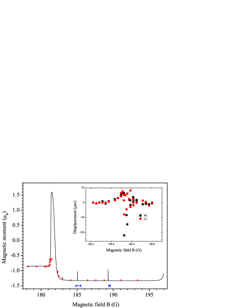
Figure 6: [Color online.] Calculated (solid line) and measured (red points) molecular magnetic moment along the magnetoassociation route starting at the 197.06 G Feshbach resonance. The two horizontal error bars mark the estimated field values for two weak avoided crossings, which we detect by variations in the cloud displacement at fixed gradient field; see inset. The crossings are visible here as spikes in the calculated curve and are indicated more explicitly in Figs. 5b and  5c. Inset: Cloud displacement as a function of magnetic field $B$ near the weak avoided crossing at $B=189.50\,$G. The strong variation in the displacement data indicates the presence of the crossing. Similar data is obtained for the weak avoided crossing near $B=185.17\,$G.

Magnetic moment spectroscopy has also allowed us to estimate the magnetic field values at which the two $|{-2}(1,3)d\rangle$ states cross the least-bound state, as shown by arrows in Fig. 5. Results for one of the crossings are shown in the inset to Fig. 6. A very small increase in the magnetic moment is seen near 189.50 G, which we interpret as a partial crossover onto $|2(1,3)d(1,1)\rangle$ during the magnetic field sweep before levitation; the corresponding avoided crossing is illustrated in Fig. 5(c). We have tried to cross over to this state adiabatically but have not been successful, most likely due to technical magnetic field fluctuations. The $|-(1,3)d(0,3)\rangle\leftrightarrow|{-1}(1,3)s(1,3)\rangle$ crossing, illustrated in Fig. 5(b), has also been observed in this way. The magnetic moment signal produced by these crossings is difficult to analyze because it is so weak, and the error bars shown in Fig. 5 simply span the range over which the magnetic moment deviates from its background value.

III.5 Bound-free modulation spectroscopy and binding energy of the $|{-2}(1,3)d(0,3)\rangle$ state

The binding energy of the $|{-2}(1,3)d(0,3)\rangle$ state proved to be difficult to measure directly, presumably due to extremely weak coupling to the atomic scattering channel. However, it was possible to observe this state in the vicinity of the crossing with $|{-6}(2,4)d(2,4)\rangle$, as shown in Fig. 5(a), using bound-free magnetic-field modulation spectroscopy Regal et al. (2003). In this version of modulation spectroscopy, molecules that are produced by magnetoassociation (as described in subsection III.3) are dissociated when the energy $hf_{\text{m}}$ corresponding to the modulation frequency $f_{\text{m}}$ is equal to or slightly greater than the binding energy. The threshold frequency at which molecules begin to be destroyed is associated with the binding energy. We observe the bound-free transition by omitting from our experimental sequence the reverse magnetoassociation ramp that is used to observe the molecules. Any atoms that appear after applying the modulation are assumed to be produced from molecule-atom transitions. Because the atomic signal background is now very low, this method has inherent signal-to-background advantages over free-bound spectroscopy, but the low number of molecules increases the statistical noise. The $|{-2}(1,3)d(0,3)\rangle$ state was observable only due to mixing with $|{-6}(2,4)d(2,4)\rangle$ near the crossover at about 2.5 MHz$\times h$ binding energy. This is consistent with the fact that no Feshbach resonance could be found for the $|{-2}(1,3)d(0,3)\rangle$ state near its predicted intersection with the incoming scattering channel. Power broadening causes the binding energy of the most deeply bound states to be underestimated. While this effect was extrapolated to zero intensity, the error bars shown in Fig. 5 reflect our best estimate of the possible systematic error that remains.

IV Theory and Calculations

The Hamiltonian for the interaction of two alkali-metal atoms may be written as

$$\frac{\hbar^{2}}{2\mu}\left[-R^{-1}\frac{d^{2}}{dR^{2}}R+\frac{\hat{L}^{2}}{R^{2}}\right]+\hat{h}_{1}+\hat{h}_{2}+\hat{V}(R),$$ (1)

where $\mu$ is the reduced mass and $\hat{L}$ is the operator for the end-over-end angular momentum of the two atoms about one another. The monomer Hamiltonians including Zeeman terms are

$$\hat{h}_{j}=\zeta\hat{\imath}_{j}\cdot\hat{s}_{j}+g_{e}\mu_{\rm B}B\,\hat{s}_{zj}+g_{n}\mu_{\rm B}B\,\hat{\imath}_{zj},$$ (2)

where $\hat{s}_{1}$ and $\hat{s}_{2}$ represent the electron spins of the two atoms and $\hat{\imath}_{1}$ and $\hat{\imath}_{2}$ represent the nuclear spins. The constants $g_{e}$ and $g_{n}$ are the electron and nuclear $g$-factors, $\mu_{\rm B}$ is the Bohr magneton, and $\hat{s}_{z}$ and $\hat{\imath}_{z}$ represent the $z$-components of $\hat{s}$ and $\hat{\imath}$ along a space-fixed $Z$ axis whose direction is defined by the external magnetic field $B$. The atomic $g$-factors were taken from the 2006 CODATA adjustment of fundamental constants Mohr et al. (2007) and the ⁸⁷Rb hyperfine constant from Bize et al. Bize et al. (1999). The Cs hyperfine constant is exact by definition.

The interaction between the two atoms $\hat{V}(R)$ is

$${\hat{V}}(R)=\hat{V}^{\rm c}(R)+\hat{V}^{\rm d}(R).$$ (3)

Here $\hat{V}^{\rm c}(R)=V_{0}(R)\hat{\cal{P}}^{(0)}+V_{1}(R)\hat{\cal{P}}^{(1)}$ is an isotropic potential operator that depends on the potential energy curves $V_{0}(R)$ and $V_{1}(R)$ for the respective $X{}^{1}\Sigma_{g}^{+}$ singlet and $a{}^{3}\Sigma_{u}^{+}$ triplet states of the diatomic molecule. The singlet and triplet projectors $\hat{\cal{P}}^{(0)}$ and $\hat{\cal{P}}^{(1)}$ project onto subspaces with total electron spin quantum numbers 0 and 1 respectively. Figure 1 shows the two potential energy curves for RbCs. The term $\hat{V}^{\rm d}(R)$ represents small, anisotropic spin-dependent couplings, which are responsible for the avoided crossings described in the experimental section and are discussed further in Section IV.3 below.

IV.1 Computational methods for bound states and scattering

The three theoretical groups working on this problem used different sets of computer codes that gave results in agreement with one another. The methods used in Hannover to interpret the Fourier transform spectra and Feshbach resonance positions are described in Ref. Pashov et al. (2007). Those used at Temple University and NIST are described in Ref. Tiesinga et al. (1998). The methods used at Durham are described below.

For the scattering and Feshbach bound states, we solve the Schrödinger equation by coupled-channel methods, using a basis set for the electron and nuclear spins in a fully decoupled representation,

$$|s_{\rm Rb}m_{s,{\rm Rb}}\rangle|i_{\rm Rb}m_{i,{\rm Rb}}\rangle|s_{\rm Cs}m_{s,{\rm Cs}}\rangle|i_{\rm Cs}m_{i,{\rm Cs}}\rangle|LM_{L}\rangle.$$ (4)

The matrix elements of the different terms in the Hamiltonian in this basis set are given in the Appendix of Ref. Hutson et al. (2008). The calculations in this paper used basis sets with all possible values of $m_{s}$ and $m_{i}$ for both atoms, truncated at $L_{\rm max}=2$ unless otherwise indicated.

Scattering calculations are carried out using the MOLSCAT package Hutson and Green (1994), as modified to handle collisions in magnetic fields González-Martínez and Hutson (2007). At each magnetic field $B$, the wavefunction log-derivative matrix at collision energy $E$ is propagated from $R=0.3$ to 2.5 nm using the propagator of Manolopoulos Manolopoulos (1986) with a fixed step size of 0.02 pm and from 2.5 to 1,500 nm using the Airy propagator Alexander and Manolopoulos (1987) with a variable step size controlled by the parameter TOLHI=$10^{-5}$ Alexander (1984). Scattering boundary conditions Johnson (1973) are applied at $R=1,500$ nm to obtain the scattering S-matrix. The energy-dependent $s$-wave scattering length $a(k)$ is then obtained from the diagonal S-matrix element in the incoming $L=0$ channel using the identity Hutson (2007)

$$a(k)=\frac{1}{ik}\left(\frac{1-S_{00}}{1+S_{00}}\right),$$ (5)

where $k^{2}=2\mu E/\hbar^{2}$. For $L=1$, this is generalized by replacing $a$ with $a_{1}^{3}$ and $k$ with $k^{3}$.

Weakly bound levels for Feshbach molecules are obtained using a variant of the propagation method described in Ref. Hutson et al. (2008). The log-derivative matrix is propagated outwards from $R=0.3$ to 2.5 nm with a fixed step size of 0.02 pm and inwards from 1,500 and 2.5 nm with a variable step size. In Ref. Hutson et al. (2008), bound-state energies at a fixed value of the magnetic field $B$ were located using the BOUND package Hutson (1993), which converges on energies where the smallest eigenvalue of the log-derivative matching determinant is zero Hutson (1994). However, for the purposes of the present work we used a new package, FIELD, which instead works at fixed binding energy and converges in a similar manner on the magnetic fields at which bound states exist. BOUND and FIELD both implement a node-count algorithm Hutson (1994) which makes it straightforward to ensure that all bound states that exist in a particular range of energy or field are located.

Zero-energy Feshbach resonances can in principle be located as fields $B_{\rm res}$ at which the scattering length $a(B)$ passes through a pole. However, with this method it is necessary first to search for poles, and it is quite easy to miss narrow resonances. Since resonances occur at fields where there is a bound state at zero energy, the FIELD package provides a much cleaner approach: simply running FIELD at zero energy provides a complete list of all fields at which zero-energy Feshbach resonances exist.

IV.2 Representation of the potential curves

The singlet and triplet curves are represented as described by Docenko et al. Docenko et al. (2011). In a central region from $R^{\rm SR}_{S}$ to $R^{\rm LR}_{S}$, with $S=0$ or 1 for the singlet or triplet state, respectively, the curves are well determined by the Fourier transform spectra and are represented as finite power expansions of a nonlinear function $\xi$ that depends on the internuclear separation $R$,

$$V_{S}(R)=hc\sum_{i=0}^{n}a_{i}\xi^{i}(R),$$ (6)

where

$$\xi(R)=\frac{R-R_{\rm m}}{R+bR_{\rm m}}.$$ (7)

The quantities $a_{i}$ and $b$ are fitting parameters, and $R_{\rm m}$ is chosen to be near the equilibrium distance. At long range ($R>R^{\rm LR}_{S}$), the potentials are

$$\begin{split}V_{S}^{\rm LR}(R)=-C_{6}/R^{6}-C_{8}/R^{8}-C_{10}/R^{10}\\ -(-1)^{S}V_{\rm exch}(R),\end{split}$$ (8)

where the dispersion coefficients $C_{n}$ are common to both potentials. The exchange contribution is Smirnov and Chibisov (1965)

$$V_{\rm exch}(R)=A_{\rm ex}(R/a_{0})^{\gamma}\exp(-\beta R/a_{0}),$$ (9)

and makes an attractive contribution for the singlet and a repulsive contribution for the triplet. $\beta$ and $\gamma$ are related via $\gamma=7/\beta-1$ and are obtained from the ionization energies of Rb and Cs Smirnov and Chibisov (1965), and $A_{\rm ex}$ is a fitting parameter. The mid-range potentials are constrained to match the long-range potentials at $R_{S}^{\rm LR}$. Lastly, the potentials are extended to short range ($R<R_{S}^{\rm SR}$) with simple repulsive terms,

$$V_{S}^{\rm SR}(R)=A^{\rm SR}_{S}+B^{\rm SR}_{S}[a_{0}/R]^{N},$$ (10)

where $A^{\rm SR}_{S}=V_{S}(R_{S}^{\rm SR})-B^{\rm SR}_{S}[a_{0}/R_{S}^{\rm SR}]^{N}$ is chosen to match the short-range and mid-range potentials at $R_{S}^{\rm SR}$.

IV.3 Magnetic dipole interaction and second-order spin-orbit coupling

At long range, the coupling $\hat{V}^{\rm d}(R)$ of Eq. 3 has a simple magnetic dipole-dipole form that varies as $1/R^{3}$ Stoof et al. (1988); Moerdijk et al. (1995). However, for heavy atoms it is known that second-order spin-orbit coupling provides an additional contribution that has the same tensor form as the dipole-dipole term and dominates at short range Mies et al. (1996); Kotochigova et al. (2000). In the present work, $\hat{V}^{\rm d}(R)$ is represented as

$$\hat{V}^{\rm d}(R)=\lambda(R)\left(\hat{s}_{1}\cdot\hat{s}_{2}-3(\hat{s}_{1}\cdot\vec{e}_{R})(\hat{s}_{2}\cdot\vec{e}_{R})\right)\,,$$ (11)

where $\vec{e}_{R}$ is a unit vector along the internuclear axis and $\lambda$ is an $R$-dependent coupling constant. This term couples the electron spins of Rb and Cs atoms to the molecular axis. In particular, it couples the even partial waves ($s$, $d$, …) with one another and does the same for the odd partial waves ($p$, $f$, …).

In the present work the second-order term was evaluated from electronic structure calculations in a manner similar to that described in Ref. Kotochigova et al. (2000), using a relativistic configuration-interaction valence bond (RCI-VB) method. The molecular wave function is constructed from atomic orbitals localized at the different atomic centers. Configuration interaction (CI) coefficients are obtained by solving a generalized eigenvalue matrix problem of the relativistic electronic Hamiltonian based on a nonorthogonal basis set. At short internuclear separations, the one-electron orbitals from different centers have considerable overlap or nonorthogonality, which gives rise to a large exchange interaction and thereby creates the bond. For large internuclear separations, the molecular wave function automatically obtains a pure atomic form, which is the correct asymptotic limit for any molecular wave function. In our version of the RCI-VB method, the atomic Slater determinants are constructed from one-electron numerical Dirac-Fock functions for occupied core and valence orbitals and numerical Sturmian functions for virtual or unoccupied orbitals. These Sturmian orbitals are obtained by solving integro-differential Dirac-Fock-Sturm equations Kotochigova and Tiesinga (2005).

For RbCs, all occupied orbitals up to the 4s² shell in Rb and the 5s² shell in Cs are defined as the core orbitals. The 4p⁶ orbitals in Rb and 5p⁶ orbitals in Cs are included in the core-valence subspace, allowing single and double excitations. The 5s, 5p, 4d, 6s, and 6p orbitals of Rb and 6s, 6p, 5d, 7s, and 7p orbitals of Cs are added to the active subspace with single, double, and triple occupancy. In addition, we included virtual Sturm 5d, 4f, 7s, and 7p orbitals of Rb and 6d, 4f, 8s, and 8p orbitals of Cs to complete the active space. Up to double occupancy is allowed for these virtual orbitals.

Our relativistic valence bond method calculates the second-order spin-orbit splitting nonperturbatively. The calculation finds the energetically lowest $\Omega=0^{-}$ and $1$ states, which correspond to the two fine-structure components of the $S=1$ $a{}^{3}\Sigma^{+}$ Born-Oppenheimer potential. We denote the relativistic potentials by $V_{S,\Omega}(R)$. The difference $V_{1,1}(R)-V_{1,0^{-}}(R)=-(3/2)\lambda(R)$ provides the second-order spin-orbit splitting shown in Fig. 7. Also shown is the strength of the spin-spin dipole interaction, which leads to a splitting between the $0^{-}$ and $1$ Born-Oppenheimer potentials with opposite sign compared to the second order spin-orbit contribution.

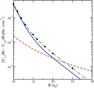
Figure 7: [Color online] Study of the second-order spin-orbit interaction energy $V_{1,1}(R)-V_{1,0^{-}}(R)$ as a function of internuclear separation $R$. The filled circles are the result of the ab initio RCI-VB electronic structure calculation. The green dash-dotted is a fit to the ab initio values using the functional form of Eq. 12. The blue line corresponds to the second-order spin-orbit interaction energy optimized to reproduce the location of the observed magnetic Feshbach resonances for A${}_{\rm 2SO}^{\rm long}$ = -0.03310. For comparison the absolute value of the corresponding splitting due to the magnetic dipole-dipole interaction is shown by a red dashed line.

The second-order spin-orbit splitting has a nearly exponential dependence on $R$ and lies about half-way between the values for Rb₂ and Cs₂ molecules calculated previously Kotochigova et al. (2000). The results of the electronic structure calculations were fitted to a biexponential form, so that the overall form of $\lambda(R)$ is

$$\lambda(R) \!\!= \!\!E_{\rm h}\alpha^{2}\bigg{[}A_{\rm 2SO}^{\rm short}\exp\left(-\beta_{\rm 2SO}^{\rm short}(R/a_{0})\right)$$ (12)

$$\!\!+ \!\!\!\!A_{\rm 2SO}^{\rm long}\exp\left(-\beta_{\rm 2SO}^{\rm long}(R/a_{0})\right)+\frac{1}{(R/a_{0})^{3}}\bigg{]},$$

where $\alpha\approx 1/137$ is the atomic fine-structure constant. The parameters obtained from fitting to the electronic structure calculations are $A_{\rm 2SO}^{\rm short}=-50.974$, $A_{\rm 2SO}^{\rm long}=-0.0525$, $\beta_{\rm 2SO}^{\rm short}=0.80$ and $\beta_{\rm 2SO}^{\rm long}=0.28$. However, in fitting to the weakly bound levels, this coupling function was found to be too strong to reproduce the avoided crossings shown in Fig. 5. We therefore retained the functional form (12) but allowed the parameter $A_{\rm 2SO}^{\rm long}$ to vary in the least-squares fit to the experimental results described below.

IV.4 Assignment of quantum numbers

At the start of this work, the singlet and triplet scattering lengths $a_{S}$ and $a_{T}$ for RbCs were unknown within wide ranges and there was no assignment of quantum numbers to the Feshbach resonances of Ref. Pilch et al. (2009). However, the identification of a bound state in the $|1,1\rangle+|3,3\rangle$ channel bound by only about 110 kHz placed the possible values of $a_{S}$ and $a_{T}$ along a well-defined curve in the upper-right quadrant of $a_{S},a_{T}$ space. We therefore used a pre-publication version of the mid-range RbCs potentials of Docenko et al. Docenko et al. (2011), modified to allow us to vary the scattering lengths, and carried out coupled-channel calculations at a number of points along this line to identify lists of $s$-wave Feshbach resonances. By altering the long-range coefficients and inner-wall parameters of this potential, we were able to produce a resonance pattern that approximately matched the experimental one, and also gave a pattern of bound states similar to that from free-bound spectroscopy. A key feature that strengthened our confidence in this assignment was that it predicted two very weak crossings between the least-bound state near 110 kHz and two $n=-2$ states, as shown in Fig. 5. The presence of these crossings was then confirmed by experiment as described in Section III.4 above.

At around this time, the final version of the spectroscopic potentials of Ref. Docenko et al. (2011) became available. These had different numbers of singlet and triplet bound states from the preliminary version, but approximately the correct scattering lengths. We therefore used this potential to produce resonance patterns and a bound state map of the region immediately below the lowest threshold. This gave a good match to the experimentally observed Feshbach resonance positions, but placed the two $n=-2$ states that cross the least-bound state between 180 G and 190 G at fields about 3 G too low. In addition, the avoided crossings between the $n=-6$ states and the least-bound state were broader than was found experimentally. We therefore embarked on a two-part least-squares refinement, beginning from the potential of Ref. Docenko et al. (2011), as described below.

IV.5 Least-squares refinement

The Feshbach bound states and resonance positions are strongly sensitive to the long-range potential and to the scattering lengths, but only weakly sensitive to the details of the potential in the well region. The Fourier Transform spectra, by contrast, are very sensitive to the well region. The potentials are determined in an iterative loop using the data sequentially, as was successfully applied for example in Ref. Pashov et al. (2007). First, in the least-squares fit to weakly bound states and Feshbach resonance positions, the potential curves in the central region were held fixed but the long-range coefficients $C_{6}$ and $C_{8}$ were allowed to vary. In addition, the parameters $B_{0}^{\rm SR}$ and $B_{1}^{\rm SR}$ were varied, allowing the inner walls of the two potential curves to move sufficiently to adjust the singlet and triplet scattering lengths independently of $C_{6}$ and $C_{8}$. The scaling factor for the long-range part of the 2nd-order spin-orbit coupling was also varied in this step. In the second step, the long-range function was held fixed and the inner parts of the potentials were varied to fit the large set of results from Fourier Transform spectroscopy, adding as data the uncoupled last-bound levels constructed from the fit in the first step. Two iterations were sufficient to achieve convergence between the two different least-squares procedures.

The propagator approach to locating bound states and resonances, implemented in the BOUND and FIELD programs, is fast enough to be incorporated in a least-squares fitting program. Nevertheless, it is still slow enough that these calculations form the major time-consuming step in a least-squares refinement procedure. Furthermore, the parameter set used is highly correlated. Under these circumstances, a fully automated approach to fitting is unreliable: individual least-squares steps often reach points in parameter space where the levels have moved too far to be identified reliably, particularly in the early stages of fitting. We therefore carried out this stage of the fitting using the I-NoLLS package Law and Hutson (1997) (Interactive Non-Linear Least-Squares), which gives the user interactive control over step lengths and assignments as the fit proceeds. This allowed us to converge on a minimum in the sum of weighted squares in a relatively small number of steps.

The measurements on weakly bound states described above complement the measurements of the positions of Feshbach resonances. In particular: (i) the position of the least-bound state is sensitive to the background scattering length in the incoming $|1,1\rangle$ + $|3,3\rangle$ channel; (ii) the strengths of the avoided crossings between the least-bound state and the ramping $n=-6$ states from the (2,4) threshold are sensitive to the magnitude of the 2nd-order spin-orbit coupling; (iii) the positions of the $n=-2$ states associated with the (1,3) threshold, observed through their avoided crossings with the least-bound state, are sensitive to the long-range $C_{6}$ coefficient, but relatively uncontaminated by the influence of $C_{8}$, which becomes important for deeper levels. In combination with the Feshbach resonances due to $n=-6$ states, whose position is significantly influenced by the $C_{8}$ coefficient, the $n=-2$ levels open the way for $C_{6}$ and $C_{8}$ to be determined separately.

Table 2: Quality of fit to Feshbach bound states and resonance positions. Top section: a complete list of the fields (in G) for all calculated $s$-wave resonances in the region 10 to 560 G using an $sd$ basis, together with quantum labels as explained in the text. Some calculated resonances have not been observed experimentally. Center section: fields used to characterize the ramping states $|-6(2,4)d(2,4)\rangle$ and $|-6(2,4)d(2,3)\rangle$ and their avoided crossings with the least-bound state. Bottom section: the binding energy of the $|-2(1,3)d(0,3)\rangle$ bound state at 181.18 G, just below its crossing with $|-6(2,4)d(2,4)\rangle$. For all states here, the total angular projection quantum number $M$ is 4. The uncertainties quoted here are those that define the weights used in our least-squares fit.

$B_{\rm calc}$		$B_{\rm obs}$	$B_{\rm obs}-B_{\rm calc}$			Unc.		quantum labels
87.25								$\left|-2\,(1,3)\,d\,(-1,3)\right\rangle$
123.09								$\left|-2\,(1,3)\,d\,(0,2)\right\rangle$
181.63		181.64		$0.01$		0.10		$\left|-6\,(2,4)\,d\,(2,4)\right\rangle$
197.07		197.06		$-0.01$		0.046		$\left|-6\,(2,4)\,d\,(2,3)\right\rangle$
217.33		217.34		$0.01$		0.047		$\left|-6\,(2,4)\,d\,(2,2)\right\rangle$
225.47		225.43		$-0.04$		0.034		$\left|-6\,(2,4)\,d\,(1,4)\right\rangle$
242.25		242.29		0.04		0.047		$\left|-6\,(2,4)\,d\,(2,1)\right\rangle$
247.28		247.32		0.04		0.048		$\left|-6\,(2,4)\,d\,(1,3)\right\rangle$
272.81		272.80		$-0.01$		0.043		$\left|-6\,(2,4)\,d\,(2,0)\right\rangle$
		273.45				0.04
273.69		273.76		0.07		0.043		$\left|-6\,(2,4)\,d\,(1,2)\right\rangle$
279.02		279.12		0.10		0.048		$\left|-6\,(2,4)\,s\,(2,2)\right\rangle$
286.68		286.76		0.08		0.047		$\left|-6\,(2,4)\,d\,(0,4)\right\rangle$
308.45		308.44		$-0.01$		0.045		$\left|-6\,(2,4)\,d\,(1,1)\right\rangle$
310.71		310.69		$-0.02$		0.056		$\left|-6\,(2,4)\,s\,(1,3)\right\rangle$
314.56		314.74		0.18		0.11		$\left|-6\,(2,4)\,d\,(0,3)\right\rangle$
352.74		352.65		$-0.09$		0.34		$\left|-6\,(2,4)\,s\,(0,4)\right\rangle$
353.57								$\left|-6\,(2,4)\,d\,(0,2)\right\rangle$
381.28		381.34		0.06		0.047		$\left|-6\,(2,4)\,d\,(-1,4)\right\rangle$
408.63								$\left|-2\,(1,3)\,d\,(1,2)\right\rangle$
422.04		421.93		$-0.11$		0.047		$\left|-6\,(2,4)\,d\,(-1,3)\right\rangle$
552.75								$\left|-6\,(2,4)\,d\,(-2,4)\right\rangle$
185.24		185.34∗		0.10		0.35		$\left|-2\,(1,3)\,d\,(0,3)\right\rangle$
189.47		189.66†		0.19		0.10		$\left|-2\,(1,3)\,d\,(1,1)\right\rangle$

	$B_{\rm calc}$	$B_{\rm obs}$	$B_{\rm obs}-B_{\rm calc}$	Unc.
$B_{(2,4)}$ at $-1.02$ MHz	181.729	181.758	0.030	0.03
$B_{(2,3)}$ at $-0.84$ MHz	196.978	196.946	$-0.019$	0.02
$B^{+}_{(2,4)}$ at $-0.030$ MHz	181.381	181.380
$B^{-}_{(2,4)}$ at $-0.210$ MHz	182.358	182.316	$-0.042$	0.03
$B^{-}_{(2,4)}-B^{+}_{(2,4)}$	0.977	0.936	$-0.041$	0.07
$B^{+}_{(2,3)}$ at $-0.030$ MHz	196.991	196.950
$B^{-}_{(2,3)}$ at $-0.185$ MHz	197.300	197.278	$-0.022$	0.03
$B^{-}_{(2,3)}-B^{+}_{(2,3)}$	0.309	0.328	0.019	0.06
	$-E_{\rm calc}$	$-E_{\rm obs}$	$-E_{\rm obs}+E_{\rm calc}$	Unc.
$E^{-2}_{(0,3)}$ at 181.18 G	2.767	2.525	$-0.242$	0.10
(MHz)

^∗ Resonance position extrapolated from avoided crossing at 185.17 G. ^† Resonance position extrapolated from avoided crossing at 189.50 G.

Once we were confident of the assignment of the weakly bound states and Feshbach resonances, we therefore carried out least-squares refinement of the potential using the I-NoLLS package in the 5-parameter space $B_{0}^{\rm SR}$, $B_{1}^{\rm SR}$, $C_{6}$, $C_{8}$, $A_{\rm 2SO}^{\rm long}$. The set of experimental results used for this stage of fitting is listed in Table 2. It consists of the magnetic fields for all the measured $s$-wave resonances, except the resonance at 273.45 G, which we attribute to a bound state of $g$ character, and is supplemented by a selection from the measurements of the binding energies: (i) two additional resonance positions for the $n=-2$ states, obtained from the positions of the avoided crossings between the $n=-2$ states and the least-bound state by a (very short) extrapolation to zero energy using the calculated slopes of the $n=-2$ states; (ii) fields at which the bound states $|{-6}(2,4)d(2,4)\rangle$ and $|{-6}(2,4)d(2,3)\rangle$ exist near 1 MHz; (iii) four fields at which bound states exist near 110 kHz, designated $B^{+}_{(m_{\rm Rb},m_{\rm Cs})}$ and $B^{-}_{(m_{\rm Rb},m_{\rm Cs})}$, just above and just below the avoided crossings between the least-bound state and the $|{-6}(2,4)d(2,4)\rangle$ and $|{-6}(2,4)d(2,3)\rangle$ states; to improve the determination of the 2nd-order spin-orbit coupling, two of these were included as field differences $B^{-}-B^{+}$ between levels just above and just below each crossing; (iv) the energy of the $|{-2}(1,3)d(0,3)\rangle$ state at 181.18 G, just below its crossing with $|{-6}(2,4)d(2,4)\rangle$. The quantity optimized in the least-squares fits was the sum of squares of residuals ((observed $-$ calculated)/uncertainty), with the uncertainties listed in Table 2.

Table 3: Potential parameters and derived quantities resulting from least-squares fitting to Feshbach bound states and resonance positions.

	fitted value		95% confidence			sensitivity
			limit
$B_{0}^{\rm SR}$ ($E_{\rm h}$)	6960	.7	710			0.5
$B_{1}^{\rm SR}$ ($E_{\rm h}$)	19793	.3	110			0.1
$A^{\rm long}_{\rm 2SO}$	$-0$	.0331	0	.0028		0.0001
$C_{6}$ ($E_{\rm h}a_{0}^{6}$)	5693	.7056	2	.2		0.0004
$C_{8}$ ($E_{\rm h}a_{0}^{8}$)	796487	.36	1900			0.3
derived	value		uncertainty
parameters
$a_{S}$ ($a_{0}$)	997		11
$a_{T}$ ($a_{0}$)	513	.3	2	.2

Table 4: Parameters of the analytic representation of the potential of state $X^{1}\Sigma^{+}$. The energy reference is the dissociation asymptote.

	$R<R_{\mathrm{SR}}=$ 0.3315 nm
$A^{\mathrm{SR}\ast}_{0}/hc$	-0.407634031$\times 10^{4}$ cm-1
$B^{\mathrm{SR}}_{0}/hc$	1.52770630$\times 10^{9}$ cm-1
$N_{0}$	7
	$R_{\mathrm{SR}}\leq R\leq R_{\mathrm{LR}}=$ 1.150 nm
$b$	$0.09$
$R_{\mathrm{m}}$	0.442708150 nm
$a_{0}$	-3836.36509 cm-1
$a_{1}$	-0.0369980716645394794 cm-1
$a_{2}$	0.447519742785341805$\times 10^{5}$ cm-1
$a_{3}$	-0.134065881674135253$\times 10^{5}$ cm-1
$a_{4}$	-0.112246913875781145$\times 10^{6}$ cm-1
$a_{5}$	-0.680373468487243954$\times 10^{5}$ cm-1
$a_{6}$	0.124395856928352383$\times 10^{6}$ cm-1
$a_{7}$	-0.527808915105630062$\times 10^{6}$ cm-1
$a_{8}$	0.160604050855185674$\times 10^{7}$ cm-1
$a_{9}$	0.856669313055434823$\times 10^{7}$ cm-1
$a_{10}$	-0.423220682973604128$\times 10^{8}$ cm-1
$a_{11}$	-0.846286860630152822$\times 10^{8}$ cm-1
$a_{12}$	0.775110557475278497$\times 10^{9}$ cm-1
$a_{13}$	0.208102060193851382$\times 10^{9}$ cm-1
$a_{14}$	-0.762262944271048737$\times 10^{10}$ cm-1
$a_{15}$	0.645280096247728157$\times 10^{10}$ cm-1
$a_{16}$	0.358089708848128967$\times 10^{11}$ cm-1
$a_{17}$	-0.685156406423631516$\times 10^{11}$ cm-1
$a_{18}$	-0.340359743040435295$\times 10^{11}$ cm-1
$a_{19}$	0.204117122912590576$\times 10^{12}$ cm-1
$a_{20}$	-0.207876500106921722$\times 10^{12}$ cm-1
$a_{21}$	0.712777331768994293$\times 10^{11}$ cm-1
	$R>R_{\mathrm{LR}}$
$C_{6}$	5693.7056 $E_{\rm h}a_{0}^{6}$
$C_{8}$	796487.36 $E_{\rm h}a_{0}^{8}$
$C_{10}$	95332817 $E_{\rm h}a_{0}^{10}$
${A_{\mathrm{ex}}}/hc$	0.37664685$\times 10^{3}$ cm-1
${\gamma}$	5.427916
${\beta}$	1.0890

^∗ This parameter is set to give continuity between the short-range and mid-range functional forms.

Table 5: Parameters of the analytic representation of the potential of state $a^{3}\Sigma^{+}$. The energy reference is the dissociation asymptote.

	$R<R_{\mathrm{SR}}=$ 0.522 nm
$A^{\mathrm{SR}\ast}_{1}/hc$	-0.500680370$\times 10^{3}$ cm-1
$B^{\mathrm{SR}}_{1}/hc$	4.34413885$\times 10^{9}$ cm-1
$N_{1}$	7
	$R_{\mathrm{SR}}\leq R\leq R_{\mathrm{LR}}=$ 1.200 nm
$b$	$0.06$
$R_{\mathrm{m}}$	0.62193776 nm
$a_{0}$	-259.33587 cm-1
$a_{1}$	0.1466188573699344914 cm-1
$a_{2}$	0.525743927693154455$\times 10^{4}$ cm-1
$a_{3}$	-0.122790966318838728$\times 10^{5}$ cm-1
$a_{4}$	0.175565797136193828$\times 10^{4}$ cm-1
$a_{5}$	0.173795490253058379$\times 10^{5}$ cm-1
$a_{6}$	-0.119112720845007316$\times 10^{5}$ cm-1
$a_{7}$	-0.245659148870101490$\times 10^{5}$ cm-1
$a_{8}$	0.303380094883701415$\times 10^{6}$ cm-1
$a_{9}$	-0.100054913157079869$\times 10^{7}$ cm-1
$a_{10}$	-0.296340813141656632$\times 10^{6}$ cm-1
$a_{11}$	0.997302450614721887$\times 10^{7}$ cm-1
$a_{12}$	-0.272673123492070958$\times 10^{8}$ cm-1
$a_{13}$	0.323269132716538832$\times 10^{8}$ cm-1
$a_{14}$	-0.147953587185832486$\times 10^{8}$ cm-1
	$R>R_{\mathrm{LR}}$
$C_{6}$	5693.7056 $E_{\rm h}a_{0}^{6}$
$C_{8}$	796487.36 $E_{\rm h}a_{0}^{8}$
$C_{10}$	95332817 $E_{\rm h}a_{0}^{10}$
${A_{\mathrm{ex}}}/hc$	0.37664685$\times 10^{3}$ cm-1
${\gamma}$	5.427916
${\beta}$	1.0890

^∗ This parameter is set to give continuity between the short-range and mid-range functional forms.

IV.6 Final potential

At the conclusion of the two-part least-squares refinement procedure described above, we arrived at the potentials given in Tables 3, 4 and 5. Table 3 gives the parameters from fitting to the Feshbach bound states and resonance positions, whereas Tables 4 and 5 give the full potentials for the singlet and triplet states, respectively.

Although the Feshbach bound states and resonance positions do allow all 5 parameters in Table 3 to be extracted, they are very highly correlated. The table therefore gives both 95% confidence limits and parameter sensitivities as defined by Le Roy Le Roy (1998). The 95% confidence limits are correlated properties that describe the uncertainty in an individual parameter, but the parameters need to be specified to within their sensitivities, not their confidence limits, in order to reproduce the results of the calculations.

The new version of the electronic potentials for the RbCs ground-state system reproduces the Fourier transform spectra as accurately as the original version of Ref. Docenko et al. (2011), with the important improvement that it can also accurately reproduce properties relating to the very top of the electronic potentials, such as Feshbach spectra. There are some remaining deviations between the observed and calculated positions of the $n=-2$ states as shown in the lower panels of Figure 5, but in view of the possible systematic errors in the corresponding measurements described in Sections III.5 and III.4 above, these are not a great cause for concern.

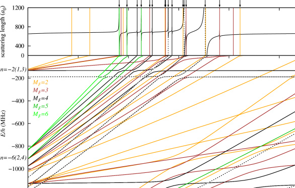
Figure 8: [Color online.] Weakly bound states of RbCs for $M=4$ at fields up to 550 G, calculated using the final fitted potentials, together with the scattering length at the $|1,1\rangle+|3,3\rangle$ threshold, calculated at $E=160$ nK. Bound states are plotted in a colour corresponding to their value of $M_{F}$, as shown on the figure. States arising from $L=2$ ($d$ states) are shown as solid lines, and from $L=0$ ($s$ states) are shown as dashed lines. The resonance positions are marked on the scattering length plot as vertical lines with the same color as the bound state that they arise from. The slanted text on the left-hand axis and below the bottom axis indicates which vibrational and hyperfine manifold the $L=2$ bound states arise from. The least-bound state $|{-1}(1,3)s(1,3)\rangle$ is within the thickness of the zero line on this scale. The observed positions of incoming $s$-wave resonances are shown as arrows above the plot.

The final results for the resonance positions and weakly bound states are listed in Table 2, together with the quality of fit to the experimental data and the quantum label assignments. The calculated $s$-wave scattering length and its match to the resonance positions is shown in Figure 8, together with an overview of the bound states responsible for the resonances.

The singlet and triplet scattering lengths $a_{S}$ and $a_{T}$ obtained from the fitted potentials are included in Table 3, together with their fully correlated uncertainties, calculated as described in Ref. Le Roy (1998). The background scattering length derived for the $|1,1\rangle+|3,3\rangle$ channel is $651\pm 10\ a_{0}$, calculated at $B=500$ G far from resonances. We have also calculated the binding energy of the least-bound state for $L=0$ at $B=211$ G (this value was chosen to represent a value far from resonance within the region for which experimental values are available) and found it to be $110\pm 2$ kHz $\times h$.

IV.7 Independent tests and predictions

IV.7.1 Resonances in $p$-wave scattering

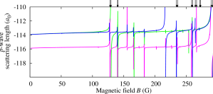
Figure 9: [Color online.] The $p$-wave scattering lengths at the $|1,1\rangle+|3,3\rangle$ threshold for the three values of $M$ allowed for $p$-wave scattering of Rb + Cs, calculated at $E=7\ \mu$K using the final fitted potentials. Results for $M_{F}=3$, 4, and 5 are shown as blue (dark gray), magenta (gray), and green (light gray), respectively. The observed positions of $p$-wave resonances are shown as arrows at the top of the graph.

As described above, some of the resonances observed by Pilch et al. Pilch et al. (2009) do not appear for the Rb+Cs mixture at the lower temperatures studied in the present work and are assigned as resonances in $p$-wave scattering. When $L_{\text{c}}=1$, $M_{L_{\text{c}}}$ can take values $-1$, 0 or +1, so $M$ can be 3, 4, or 5 at the $|1,1\rangle+|3,3\rangle$ threshold with $M_{F}=4$. Figure 9 compares the observed $p$-wave resonance positions with the $p$-wave scattering lengths for these three values of $M$, calculated using the fitted potentials. It may be seen that the observed resonances correspond quite well to a subset of the calculated resonances, although it is not altogether clear why Pilch et al. Pilch et al. (2009) observed some $p$-wave resonances and not others.

IV.7.2 Resonances at the $|2,-1\rangle+|3,3\rangle$ threshold

In addition to the resonances at the lowest threshold, Pilch et al. Pilch et al. (2009) observed two resonances at an excited threshold with the Rb atoms in their $|2,-1\rangle$ state, at 162.3 and 179.1 G. At this threshold inelastic scattering is possible, and trap loss can occur through either 2-body or 3-body collisions. The scattering length is complex, $a(B)=\alpha(B)-i\beta(B)$, and the inelastic collision rate is proportional to $\beta(B)$. Fig. 10 shows the real and imaginary parts of the $s$-wave and $p$-wave scattering lengths at this threshold, calculated using the fitted potentials, and compares them to the experimental resonance positions. It may be seen that the two observed resonances are in good agreement with the calculation, with the high-field resonance arising from $s$-wave scattering and the low-field resonance from $p$-wave scattering.

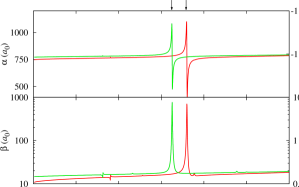
Figure 10: [Color online.] The real and imaginary parts of the complex scattering length at the Rb $|2,-1\rangle$ + Cs $|3,3\rangle$ threshold, calculated using the final fitted potentials: $s$-wave (red, dark gray, left-hand axis) and $p$-wave (green, light gray, right-hand axis). The observed resonance positions are shown as arrows at the top of the graph. The three components of the $p$-wave scattering length are indistinguishable on this scale.

IV.7.3 Unassigned resonance

As noted above, there is one resonance observed in $s$-wave scattering, at 273.45 G, that does not appear in coupled-channel calculations on the fitted potential using a basis set with $L_{\rm max}=2$. However, there are numerous additional resonances that appear when basis sets including more partial waves are used. In particular, a calculation including $L=4$ functions yields an additional resonance at 275.07 G that arises from the $\left|-6\,(2,4)\,g\,(-2,4)\right\rangle$ state. The exact position of this resonance is quite sensitive to variations of the potential within its uncertainty and is plausibly responsible for the otherwise unassigned resonance.

IV.7.4 High-field scattering

The resonances listed in Table 2, at fields up to 553 G, include all those expected from $|{-6}(2,4)d\rangle$ states. However, there are additional resonances that appear at higher field, mostly due to $s$ and $d$ states of $|{-5}(2,3)\rangle$. Some of the corresponding bound states appear in Fig. 8. Figure 11 shows the $s$-wave scattering length at fields up to 1000 G; in particular, the comparatively wide resonance near 790 G (with width $\Delta=4.2$ G) is due to the $|{-5}(2,3)s(2,2)\rangle$ state. This wide resonance may be useful for tuning interspecies scattering properties, and for studying few-body properties such as interspecies Efimov resonances Kraemer et al. (2006). In particular, since there is a very broad Feshbach resonance for Cs in state $|3,3\rangle$ with a pole at $787$ G Berninger et al. (2011), Rb+Cs mixtures may make it possible to study Efimov physics near overlapping Feshbach resonances.

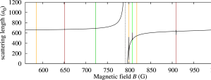
Figure 11: [Color online.] RbCs scattering length at the $|1,1\rangle+|3,3\rangle$ threshold at fields above 560 G, calculated at $E=160$ nK using the final fitted potential. Resonance positions are marked by vertical lines, with the value of $M_{F}$ of the corresponding bound state indicated using the same color scheme as in Fig. 8.

V Outlook

We have studied and modeled interspecies scattering in an ultracold Rb-Cs gas mixture with the aim of finding an assignment for the observed interspecies Feshbach resonances and in particular to understand the spectrum of weakly bound RbCs molecules.

Our results are of great importance for the production of ultracold samples of heteronuclear molecules and for the generation of dipolar quantum gases made of RbCs molecules. With recent work on optical one- and two-photon spectroscopy Debatin et al. (2011) we are now poised to perform stimulated ground-state transfer using the STIRAP technique. We expect that a three-dimensional optical lattice will allow us to maximize the molecule creation and state transfer efficiencies, as in recent work on Cs₂ Danzl et al. (2010). As detailed in Ref. Lercher et al. (2011), interspecies Feshbach tuning will be used to bring a superfluid sample of Rb atoms into overlap with a single-atom-per-site Mott insulator for Cs, in order to optimize the Rb-Cs pair-creation efficiency. With sufficiently high efficiencies, the creation of a dipolar quantum gas of RbCs molecules is within reach.