Sampling properties of directed networks

Abstract

For many real-world networks only a small “sampled” version of the original network may be investigated; those results are then used to draw conclusions about the actual system. Variants of breadth-first search (BFS) sampling, which are based on epidemic processes, are widely used. Although it is well established that BFS sampling fails, in most cases, to capture the IN-component(s) of directed networks, a description of the effects of BFS sampling on other topological properties are all but absent from the literature. To systematically study the effects of sampling biases on directed networks, we compare BFS sampling to random sampling on complete large-scale directed networks. We present new results and a thorough analysis of the topological properties of seven different complete directed networks (prior to sampling), including three versions of Wikipedia, three different sources of sampled World Wide Web data, and an Internet-based social network. We detail the differences that sampling method and coverage can make to the structural properties of sampled versions of these seven networks. Most notably, we find that sampling method and coverage affect both the bow-tie structure, as well as the number and structure of strongly connected components in sampled networks. In addition, at low sampling coverage (i.e. less than 40%), the values of average degree, variance of out-degree, degree auto-correlation, and link reciprocity are overestimated by 30% or more in BFS-sampled networks, and only attain values within 10% of the corresponding values in the complete networks when sampling coverage is in excess of 65%. These results may cause us to rethink what we know about the structure, function, and evolution of real-world directed networks.

I Introduction

In the last decade, a flood of research on systems that can be represented as networks has revealed that most differ markedly from simple random graph models Strogatz2001 ; Albert2002 ; Dorogovtsev2002 ; Newman2003 . For example, many exhibit a broad, or “scale-free” degree distribution, making them robust to random failures but rendering them vulnerable to targeted attacks Albert2000 ; Cohen2000 ; Cohen2001 . Complex networks research also offers a framework for representing biological processes such as gene regulation Davidson2002 , protein-protein interactions HJeong2001 ; Mering2002 , and even connections between diseases and symptoms KGoh2007 ; Yildirim2007 . Our growing understanding of how epidemics spread on networks has led to parallel insights into the propagation of information, fashions, ideas, and fads Grassberger1983 ; PastorSatorras2001 ; PastorSatorras2001a ; Zanette2001 ; Kuperman2001 ; Moreno2004 ; Lind2007 . Complex network studies have incorporated features such as the weight and direction of links to describe systems more precisely. Link directionality plays a particularly important role in dynamics, as small changes to link structure can completely change the dynamics on a network DUHwang2005 ; Nishikawa2006 ; SMPark2006 ; SWSon2009 . Thus, capturing the directional structure is essential to understanding the dynamics on directed networks, much as the connectivity structure is essential to dynamic processes on undirected networks.

One impediment, however, is that it is difficult, if not impossible, to obtain a complete list of links for many networks, including, for example, the World Wide Web (WWW) or large-scale gene-regulatory networks. The Web changes so quickly that by the time one could have covered it, it would be substantially transformed Ntoulas2004 ; WWWSize . Even if one somehow managed to completely map its structure at some point in time, analyzing such a large network, estimated to contain at least 19 billion pages WWWSize , would present further impediments. There is no way to avoid biases because the Web can only be sampled by following directional hyperlinks, which leaves portions inaccessible. Furthermore, as has been found to be the case with sampled, undirected networks, the sampled Web’s appearance might even fundamentally change depending on the type of sampling method used SamplingBook ; Newman2003a . If we are to have a clear and reliable picture of large-scale directed networks and their statistical properties, it is important that we quantitatively understand the effects of sampling biases on the properties of interest, as well as why such biases arise. Insight into these questions stands to impact structure-exploiting search and ranking algorithms, such as Google’s PageRank PageRank ; Son2012 , and may cause us to rethink what we know about the structure, function, and evolution of real-world networks.

Up to now the statistical properties of sampled undirected networks have been investigated in several papers. Stumpf et al. Stumpf2005 ; Stumpf2005a studied the degree distribution of two random networks – one that had been sampled “uniformly” by picking nodes at random, and one that was subject to connectivity-dependent sampling – both analytically and numerically. Lee et al. SHLee2006 also studied, numerically, the effects of random sampling and snowball sampling snowball , on statistical properties of real scale-free networks – including degree distribution exponents, betweenness centrality exponents, assortativity, and clustering coefficient – demonstrating that these quantities could be either overestimated or underestimated, depending on the fraction of the network sampled and the type of sampling method used. Kurant et al. Kurant2010 ; Kurant2011 provided a detailed analytic treatment of measurement bias due to random sampling and breadth-first search (BFS) sampling BFS , showing that, for example, BFS sampling can lead to overestimation of average degree, and random sampling to underestimation.

In the case of directed networks, however, even though the structural properties of many directed real-world networks have been examined Dorogovtsev2001 ; Garlaschelli2004 ; Bianconi2008 ; Leicht2008 ; Donato2008 , much less work has addressed the statistical properties that result from sampling them Becchetti2006 ; Wangt2010 . The majority of numerical studies in these works were not performed at a level of rigor sufficient to produce meaningful statistics. Also, the researchers began their studies with already-biased network data since they were obtained using a web crawler.

For these reasons, we investigate the biases induced by sampling large-scale directed networks starting with complete networks that differ from one another structurally. Several structural properties such as average degree, variance in degree, degree auto-correlation, reciprocity, assortativity, and component structure – all of which are defined in later sections – are analyzed to give a more complete picture of sampling-induced biases. Because we know the full, final structure we can accurately measure how systematic errors in measured quantities are affected by sampling coverage and sampling method. We find that the earlier conclusions in SHLee2006 ; Kurant2011 regarding biases in average degree of undirected networks due to random sampling and BFS sampling also hold for directed networks. On the other hand, in direct contradiction with Becchetti2006 , we conclude that both random sampling and BFS sampling overestimate edge reciprocity in the networks we study. We show that both sampling methods overestimate degree auto-correlation, sometimes by nearly 400%. In addition, we find that random sampling and BFS sampling affect the variance of in- and out-degree differently: both are underestimated by random sampling while variance in in-degree is underestimated and variance in out-degree overestimated by BFS sampling. Finally, we expand on the work in Becchetti2006 by providing a thorough examination of component sizes and abundances under random sampling and BFS sampling.

In Sec. II, we define the large-scale structural properties of directed networks, the so-called “bow-tie” structure Broder2000 , and introduce the complete networks studied in this work. We also provide a detailed accounting of the sampling methods used. In Sec. III, we present results for BFS sampling and uniform, random sampling on these networks and, where possible, provide arguments regarding how sampling can lead to measurement bias. We systematically study how accuracy is affected by the fraction of the network sampled in the two cases. Finally, summary and concluding remarks are given in Sec. IV.

II Properties of Directed Networks

II.1 Directed Networks and Bow-Tie Structure

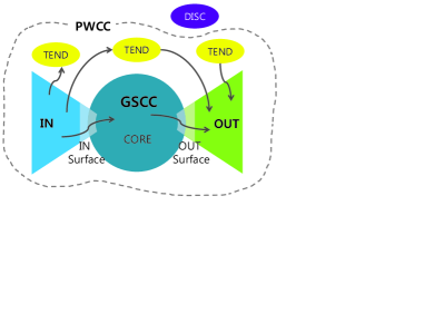
Figure 1: (Color online) Schematic of components and surfaces of a directed network. The giant strongly connected component (GSCC) and the in- and out-components (IN and OUT) account for the “bow-tie” structure. Together with tendrils (TEND), these components form the primary weakly connected component (PWCC). Portions of the network that are not connected to the PWCC are disconnected components (DISC). Nodes of the GSCC that are directly connected to nodes of IN or OUT form the surface of the GSCC; the nodes in IN or OUT to which GSCC surface nodes connect form the IN and OUT surfaces.

Table 1: Summary of component ratios for the data sets. $N_{0}$ is the total number of nodes in the networks, $N_{SCC}$ is the number of SCCs in the networks, and the component ratios mean how many nodes are placed in each component. Surface nodes ratio is the percentage of the surface nodes.

Network	$N_{0}$	$N_{\rm SCC}$	Components (%)				Surface Nodes (%)
			GSCC	OUT	IN	TEND	in GSCC	in PWCC
BerkStan	654,782	107,858	51.1	19.1	24.4	5.4	9.6	20.0
Google	855,802	355,451	50.8	19.4	21.1	8.7	41.9	52.2
Stanford	255,265	29,157	59.0	26.4	12.8	1.7	7.4	18.3
RaySoda	17,852	10,455	39.6	14.1	39.6	6.7	75.3	80.8
Wiki2005	1,596,970	490,715	69.1	2.2	28.6	0.1	43.5	59.8
Wiki2006	2,935,761	928,028	68.3	1.5	30.1	0.2	45.1	61.1
Wiki2007	3,512,462	1,148,923	67.2	1.4	31.4	0.1	46.5	62.4

If one explores a directed network by following links, some portions of the network are reachable while other portions may not be. It might be possible to go from one site to another, while the return journey is impossible. This results in a component picture of a directed network, as shown in Fig. 1. We can define a set of nodes among which a path both to and from all other nodes in the set exists. This is a strongly connected component (SCC) Tarjan1972 . A directed network can be decomposed into SCCs if isolated nodes, or nodes with only a single incoming or outgoing link are considered to be their own SCC. Then Tarjan’s algorithm Tarjan1972 can be easily modified to identify the network’s SCCs. The largest SCC is called the giant strongly connected component (GSCC), and corresponds to the knot in the so-called bow-tie structure Broder2000 . However, we can also ignore link directionality and identify the sets of nodes that are connected. These are weakly connected components (WCC). A fragmented network may contain several WCCs; the largest of these is called the giant weakly connected component (GWCC) Dorogovtsev2001 and the WCC which contains the GSCC is defined as the primary weakly connected component (PWCC). Usually the PWCC is identical to the GWCC.

The out-component(s) (OUT) of a network are found by starting from the GSCC and following outgoing links. All those nodes that can be reached from the GSCC but that do not have paths back are part of an out-component. Conversely, all nodes that can reach the GSCC following directed links, but that cannot be reached from it form the in-component(s) (IN) of the network. The IN and OUT correspond to the two wings of the bow-tie, shown in Fig. 1. All other nodes that are in the PWCC but that are not themselves part of the GSCC, IN, or OUT form tendrils (TEND). (Note that our definition of TEND is not the same as in previous works Becchetti2006 ; Broder2000 , as we include within tendrils what they call tubes – direct bridges between IN and OUT.) Any other nodes in the network must be disconnected from the PWCC and are therefore said to be disconnected components (DISC). The GSCC connects with IN and OUT through surfaces of these components. The GSCC-surface is comprised of the nodes in the GSCC that share links with nodes in IN or OUT components; nodes in IN that adjoin the GSCC form the IN-surface; and the nodes in OUT that abut the GSCC form the OUT-surface. The set of nodes in the GSCC, excluding the surface nodes, is its core Donato2008 ; Levene2004 (see Fig. 1). Cores for IN and OUT can also be defined. Broder et al. reported that $~{}30\%$ of their sampling of the WWW is GSCC, while IN and OUT each have roughly 23% of the nodes Broder2000 . This type of result varies strongly from network to network. Such differences between many real-world, directed networks are pointed out in the next section.

II.2 Data Sets

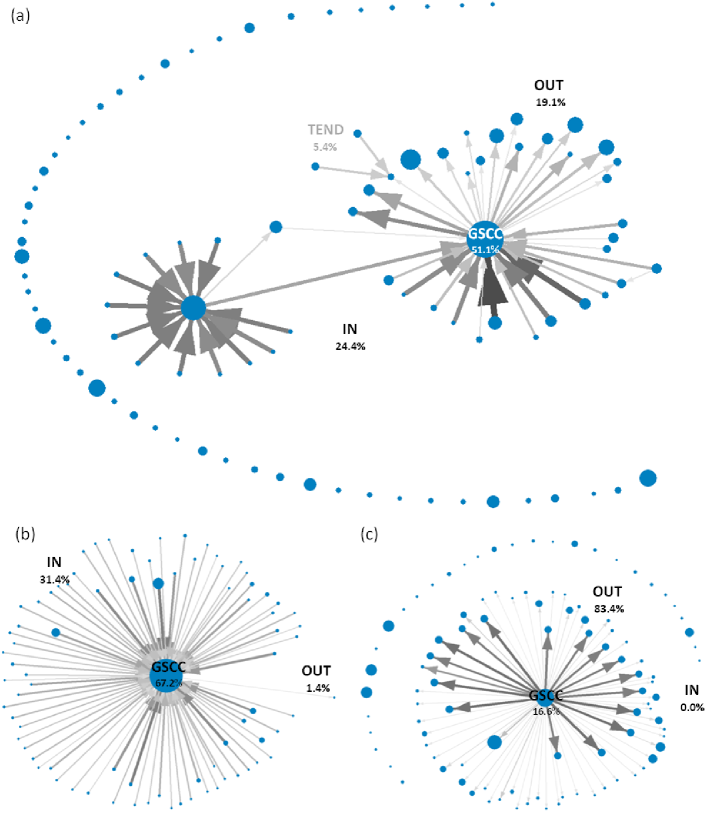
Figure 2: (Color online) SCC diagram for (a) BerkStan data StanfordDataset ; Leskovec2008 , (b) Wiki2007 WikiDataset , and (c) Notre Dame data Albert1999b (not otherwise analyzed, but shown here for its distinctive structure). For better visualization, only the 100 largest SCCs have been displayed. Each circle corresponds to a SCC, whose size is proportional to the logarithm of the number of nodes in the SCC. The width and intensity of the color of the directed links are proportional to their weight, and self-links are omitted. This SCC diagram shows the heterogeneity that can exist for the simple bow-tie diagram.

Table 2: Summary of the basic network properties for the data sets. $N_{0}$ is the number of nodes in the GWCC; $\langle k_{\rm in(out)}\rangle$ is the average incoming (outgoing) degree, always $\langle k_{\rm in}\rangle=\langle k_{\rm out}\rangle$; $\sigma^{2}_{\rm in}$ and $\sigma^{2}_{\rm out}$ are the variances of in- and out-degree, respectively; $r_{a}$ is the degree auto-correlation; $R$ is the global reciprocity; and $r_{\rm ii}$, $r_{\rm io}$, $r_{\rm oi}$, and $r_{\rm oo}$ are the in-degree/in-degree, in-degree/out-degree, out-degree/in-degree, and out-degree/out-degree assortativities.

Network	$N_{0}$	$\langle k_{\rm in}\rangle$	$\sigma^{2}_{\rm in}$	$\sigma^{2}_{\rm out}$	$r_{a}$	$R$	$r_{\rm ii}$	$r_{\rm io}$	$r_{\rm oi}$	$r_{\rm oo}$
BerkStan	654,782	11.45	84,871.8	276.3	0.043	0.244	-0.011	0.036	-0.184	0.481
Google	855,802	5.92	1,573.0	43.9	0.136	0.306	-0.014	0.033	-0.066	0.056
Stanford	255,265	8.75	30,532.2	137.6	0.046	0.262	-0.013	0.007	-0.134	0.031
RaySoda	17,852	9.47	2,995.3	268.2	0.331	0.202	-0.048	0.048	-0.125	0.093
Wiki2005	1,596,970	12.37	43,931.4	985.1	0.203	0.122	-0.014	0.017	-0.070	-0.032
Wiki2006	2,935,761	12.69	56,821.4	1,095.8	0.196	0.118	-0.008	0.014	-0.051	-0.034
Wiki2007	3,512,462	12.82	63,526.7	1,101.7	0.198	0.118	-0.007	0.013	-0.048	-0.032

We analyze seven networks: three sampled Web data sets from different sources, one complete social network, and three versions of the entire English language Wikipedia network. The Web data is a combined set of Web pages from the University of California Berkeley (berkeley.edu) and Stanford University (stanford.edu), denoted by “BerkStan”, Web pages solely from Stanford University (stanford.edu), denoted by “Stanford”, and a set of Web pages released by Google in 2002 as a part of the Google Programming Contest. All three of these data sets are available for download from the Stanford Large Network Dataset Collection StanfordDataset ; Leskovec2008 . In addition, we have gathered social network data from an amateur photographers’ website, RaySoda RaySoda , where each node corresponds to a photographer, and where a directed link from A to B indicates that A follows B. The largest networks we analyze are the Wikipedia networks Wikipedia ($\sim\mathcal{O}(10^{6})$ nodes) – three networks collected at different times (2005, 2006, and 2007). These networks, downloaded from WikiDataset , contain nodes representing five types of Wikipedia page: articles, categories, portals, disambiguations, and redirects note . The number of nodes in our networks is different from those in Buriol2006 since the networks in Buriol2006 contain only article pages, while ours contain the full collection of pages in the “main” name space of Wikipedia.

We have elected these seven networks for analysis, not only because they vary substantially in size, but also because they have different structural properties. As can be seen in Fig. 2 and Table  1, the relative sizes of components can span a wide range: the BerkStan data epitomize the classical bow-tie, with the bulk of nodes residing in the GSCC and the remainder balanced between IN and OUT; the Wikipedia networks, on the other hand, display almost no OUT, but instead show a tendency for roughly 67% of the nodes to comprise the GSCC, and the rest, the IN; conversely, the nodes of the Notre Dame data Albert1999b (which is shown in Fig. 2(c) for comparison, but is otherwise not analyzed in this paper), depicting webpages within the nd.edu domain tend to concentrate in the OUT, revealing no IN and a GSCC containing less than 20% of the network’s mass. This structure reflects how that dataset was obtained: webpages were gathered by crawling outward from a particular starting page.

Remarkably, even with these strong differences in gross global structure, we find, as shown in the next sections, many common trends in the effects of sampling biases on the measured properties of these networks. For all data sets, basic network properties, including degree distributions, average degree, variance in in- and out-degrees, degree auto-correlation, reciprocity, and four types of assortativity, are determined, and these properties, as well as component analyses, are defined and presented in corresponding subsections on sampling. All basic properties are summarized in Tables 1 and 2, and the values reported therein are later used for comparison with our sampling studies. Because it will be necessary to avoid trivial sampling failures (resulting from, for example, network disconnectedness), we consider for analysis only the GWCC of each network, which by virtue of the fact that, in all cases, it contains more than 90% of the network, is also the PWCC.

II.3 Sampling Methods

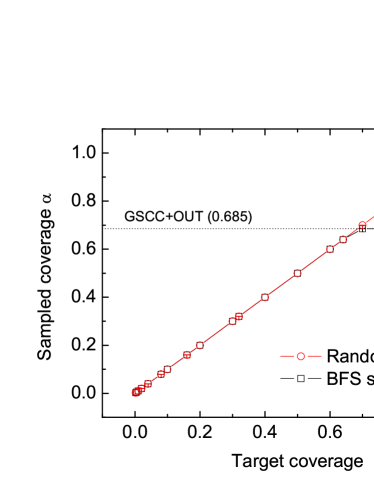
Figure 3: (Color online) Sampled coverages using two different sampling methods. While random sampling is able to achieve the targeted coverage, in most cases, BFS only covers up to the size of the GSCC and OUT. The graph shows the 2007 Wikipedia data which contains 3,512,462 nodes, and for which the combined fraction of nodes in GSCC and OUT is about 68.5%.

We use two sampling methods: uniform random sampling and breadth-first search (BFS) sampling. For the former, each node is selected independently and with equal probability. This method is not feasible on the real WWW, but it is a good basis for comparison since it is analytically tractable and is related to well-known percolation phenomena Albert2000 ; Cohen2000 ; Cohen2001 . The latter method is more complex but has been broadly adopted for web crawling, and so is important to analyze SamplingBook ; Newman2003a ; Kurant2010 ; Kurant2011 . Starting from a few randomly-selected nodes (seeds), neighboring nodes connected by outgoing links are visited at each successive step like a process of gossip spreading Lind2007 . At the outset, the seeds are added to the BFS queue. One at a time, the outgoing links of these seeds are explored, and the visited neighbours are added to the queue. We define the growing front nodes to be those nodes in the sampled network whose outgoing links have not yet been explored – i.e. those nodes most recently added to the queue. Before sampling begins, a targeted sampling coverage – the fraction of the network one wishes to sample – is also chosen. When this coverage is reached, the process terminates and all edges connecting already visited nodes are included as part of the final sampled network. This procedure is analogous to web crawling, initiating with several portal pages from which Web pages are iteratively gathered.

While BFS sampling will always cover the entire network in an undirected (connected) network, this is not the case when BFS is used to sample directed networks. In the worst case scenario, if one chooses as a starting node a node with no outgoing links, the procedure cannot proceed to the next step. We always choose $n=10$ seed nodes as starting nodes both to decrease the likelihood of this type of failure and to minimize the effects of interference between random and BFS sampling. When we sample $N$ nodes from among the $N_{0}$ nodes of the real network in order to achieve a sampling coverage, $\alpha=N/N_{0}$, randomly selecting $n$ nodes as seeds affects the sampling properties of BFS, so that as $n\to N$, BFS sampling simply becomes random sampling.

In this paper, we consider coverages of 0.25% to 100%. Mostly the sampled coverage matches the target coverage as shown in Fig. 3. However, because BFS sampling gathers new nodes by successively exploring nodes’ outgoing neighbours, its coverage cannot exceed the combined size of the GSCC and OUT, which may relate with the “reachability” in directed networks Lind2007 . We analyze all properties of the sampled network as a function of the sampled coverage $\alpha$. For every coverage, each sampling method was executed one hundred times on each network.

II.4 Sampling Measurements

We measure the following directed network properties: average degree $\langle k\rangle$, variances of incoming and outgoing degrees ($\sigma^{2}_{\rm in}$, $\sigma^{2}_{\rm out}$), degree auto-correlation $~{}r_{a}$ Dorogovtsev2002 ; Newman2003 , link reciprocity $R$ Garlaschelli2004 , and four kinds of assortativity ($r_{\rm ii}$, $r_{\rm io}$, $r_{\rm oi}$, and $r_{\rm oo}$) JFoster2010 . These will be defined in corresponding subsections. In addition, SCC analyses are performed, and we study how the SCCs and bow-tie structure change in response to sampling. For each sampling coverage, we record the ratios between the sizes of the GSCC, OUT, IN, TEND, and DISC, as well as how many nodes comprise these components’ surfaces – i.e., their points of contact Donato2008 ; Levene2004 . We further measure how, for BFS, the growing front ratio depends on $\alpha$. All the basic measurements for the complete data sets are summarized in Tables 1 and 2 as a baseline to compare with sampling results.

III Sampling Results

III.1 Average Degree and Degree Variances

Each node $i$ in a directed network has a number, $k_{\rm in}^{i}$, of incoming links (pointing to the node) and a number, $k_{\rm out}^{i}$, of outgoing links (pointing away from the node). The average total degree of a directed network is $\langle k\rangle=\langle k_{\rm in}\rangle+\langle k_{\rm out}\rangle$, where $\langle k_{\rm in}\rangle=N^{-1}\sum_{i\in\mathbb{V}}k^{i}_{\rm in}$, and similarly for $\langle k_{\rm out}\rangle$. Here $N$ is the number of sampled nodes in the network and $\mathbb{V}$ is the set of sampled nodes. Of course, $\langle k_{\rm in}\rangle=\langle k_{\rm out}\rangle={\langle k\rangle}/{2}$. The variances for in- and out-degrees are $\sigma_{\rm in}^{2}=N^{-1}\sum_{i\in\mathbb{V}}(k^{i}_{\rm in})^{2}-\langle k_{\rm in}\rangle^{2}$, and $\sigma_{\rm out}^{2}$ is similarly defined. Each network has a broad in-degree distribution and a narrower out-degree distribution. Therefore all networks exhibit a higher variance of in-degree than that of out-degree as indicated in Table 2.

For undirected networks, in the case of uniform random sampling, the sampled degree distribution $p^{\prime}(k)$ can be written as,

$$p^{\prime}(k)=\sum_{k_{0}=k}^{\infty}p(k_{0}){k_{0}\choose k}\alpha^{k}(1-\alpha)^{k_{0}-k},$$ (1)

where $p(k)$ is the degree distribution of the original network and $\alpha$ is the sampled coverage Cohen2000 ; Stumpf2005 ; Stumpf2005a ; SHLee2006 . Equation (1) also describes the incoming and outgoing degree distribution of randomly sampled directed networks, where $k$ and $k_{0}$ are replaced with $k_{\rm in}$ and $k_{0,\rm in}$ (or $k_{\rm out}$ and $k_{0,\rm out}$ respectively). The average degree of the sampled network, $\langle k\rangle^{\prime}$, is

$$\langle k\rangle^{\prime} = \sum_{k=1}^{\infty}kp^{\prime}(k)=\alpha\sum_{k_{0}=1}^{\infty}k_{0}p(k_{0})=\alpha\langle k\rangle,$$ (2)

where $\langle k\rangle$ is the average degree of the original network.

The variance of the degree under uniform random sampling is obtained from

$$\langle k^{2}\rangle^{\prime} = \sum_{k=1}^{\infty}k^{2}p^{\prime}(k)=\alpha^{2}\langle k^{2}\rangle+\alpha(1-\alpha)\langle k\rangle,$$ (3)

giving

$$\sigma^{\prime 2} = \langle k^{2}\rangle^{\prime}-\left(\langle k\rangle^{\prime}\right)^{2}=\alpha^{2}\langle k^{2}\rangle+\alpha(1-\alpha)\langle k\rangle-\alpha^{2}\langle k\rangle^{2}$$ (4)

$$= \alpha^{2}\sigma^{2}+\alpha(1-\alpha)\langle k\rangle$$

where $\sigma^{2}$ represents the variance in degree of the original network. The same formulas, Eqs. (3) and (4), also hold for the variances of the in- and out-degree, respectively. Thus $\sigma_{\rm in}^{\prime 2}$ and $\sigma_{\rm out}^{\prime 2}$ are both quadratic functions of $\alpha$, although with different coefficients ($\sigma_{\rm in}^{2}\neq\sigma_{\rm out}^{2}$). When the coverage $\alpha$ is small, $\sigma^{\prime 2}$ increases linearly with $\alpha$; for large $\alpha$ it increases quadratically.

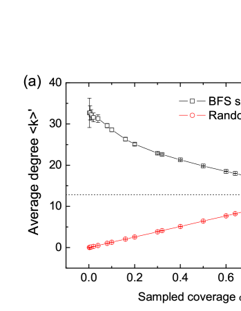
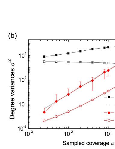
Figure 4: (Color online) Behaviors of the average degree (a) and the variance of the in-degree and out-degree (b) as a function of sampling coverage, $\alpha$, for each sampling method in the Wiki2007 data. (a) In the case of BFS sampling, the average degree approaches its asymptotic value– the average degree of the combined GSCC and OUT– from above, since BFS is biased to the high degree nodes. The average degree for random sampling is just linearly proportional to the sampling coverage. (b) The variances for in- and out-degrees for random sampling increase quadratically as sampled coverage increases, but those of BFS approach their real values from opposite directions. The gray lines behind the random sampling data are calculated from Eq. (4). Hereafter all the error bar means the standard deviation of the measured variables over sampling realizations.

This quadratic relation is shown for Wiki2007 in Fig. 4(b). The gray lines behind the random sampling data indicate the results calculated from Eq. (4). Since the variance of the incoming degree is much larger than the average degree, $\sigma_{\rm in}^{\prime 2}$ seems to be purely quadratic in this plot, but the variance of the outgoing degree, $\sigma_{\rm out}^{\prime 2}$, shows the transition from a linear to a quadratic function as $\alpha$ increases. As can be seen in Fig. 4(b), random sampling severely underestimates variances of in- and out-degree (by as much as two orders of magnitude even at $\sim 10\%$ coverage). This underestimation results from the quadratic dependence of Eq. (4) on $\alpha$.

As shown in Fig. 4, BFS sampling does not obey these simple mathematical relationships. Since BFS follows outgoing links and reaches hub nodes at early times SHLee2006 ; Becchetti2006 , one could have an argument that the average degree of BFS-sampled networks overestimates the average degree. However, this can only be true when the networks contain loops. In the case of a tree, since the network resulting from BFS sampling is still a tree, the average degree is $2-\frac{2}{N}$ very close to $\langle k\rangle=2-\frac{2}{N_{0}}\approx 2$. The average degree of BFS-sampled networks is related to the loop structures and clustering. Therefore we measure the size of the growing front under BFS sampling and the number of directed links pointing into the already sampled networks as shown in Figs. 5(a) and (b). In early stages of BFS sampling, although most nodes lie in the growing front, the fraction of their links pointing back to the already sampled nodes is surprisingly high.

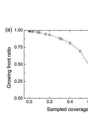
Figure 5: (Color online) For BFS sampling of Wiki2007 data, (a) growing front ratio as a function of coverage and (b) directed links ratio (the fraction of edges in the growing front that point outside (circles) or back into (squares) the already sampled network). Note that even for small coverage a substantial fraction of links directing from the growing front point back to the already sampled network.

BFS sampling also overestimates variance of out-degree, but underestimates variance of in-degree as can be seen in Fig. 4(b). However, these errors are less severe than for random sampling. Variance of in-degree is underestimated in BFS sampling for the same reason it is underestimated in random sampling, although the misestimations are less severe since the correlated loop structures affects the directed link ratio of the growing front as shown in Fig. 5(b). Variance in out-degree is overestimated for a different reason: visited nodes have the same out-degree in the sampled networks as they do in the original networks, while the out-degree of growing front nodes is not fully counted. As $\alpha$ increases, the effect of the growing front nodes diminishes. Indeed the fraction of directed (and unexplored) links pointing outside of the sampled network shrinks quickly even though the fraction of nodes on the growing front decreases much more slowly, as shown in Fig. 5(a) and (b).

III.2 Degree Auto-correlation

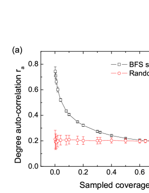
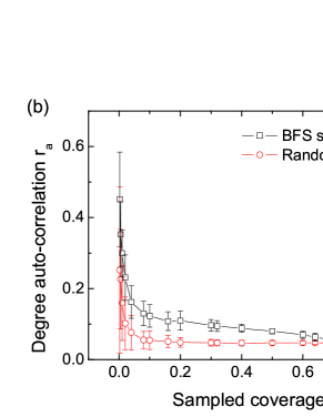
Figure 6: (Color online) Degree auto-correlation for (a) Wiki2007 data and (b) Stanford data under both sampling methods. BFS sampling significantly overestimates this quantity.

Table 3: Summary of incoming and outgoing degree and average local reciprocity for each component. Here $\langle\cdot\rangle$ means the average over nodes in each component.

Component	Wiki2007				Google
	size (%)	$\langle k_{\rm in}\rangle$	$\langle k_{\rm out}\rangle$	$\langle R_{i}\rangle$	size (%)	$\langle k_{\rm in}\rangle$	$\langle k_{\rm out}\rangle$	$\langle R_{i}\rangle$
GSCC	67.2	18.72	17.76	0.122	50.8	9.51	8.40	0.330
OUT	1.4	15.88	0.04	0.0004	19.4	3.46	1.35	0.292
IN	31.4	0.11	2.84	0.006	21.1	1.47	5.87	0.188
TEND	0.1	1.06	0.44	0.090	8.7	1.25	1.76	0.190
GWCC	100.0	12.82		0.118	100.0	5.92		0.306

Degree auto-correlation quantifies the extent to which nodes of high in-degree also have high out-degree, and is defined as $r_{a}={\rm Cov}(k_{\rm in},k_{\rm out})/\sigma_{\rm in}\sigma_{\rm out}$. The covariance is given by, ${\rm Cov}(k_{\rm in},k_{\rm out})=N^{-1}\sum_{i\in\mathbb{V}}k_{\rm in}^{i}k_{\rm out}^{i}-\langle k_{\rm in}\rangle\langle k_{\rm out}\rangle$. All networks, except for BerkStan and Stanford, have moderately high degree auto-correlation ($r_{a}>0.1$).

In the case of random sampling, the degree auto-correlation, $r_{a}$, is unbiased if $\alpha$ is large enough to ensure an adequate density of links, since the in- and out-degrees for each node are sampled randomly. Figures 6(a) and (b) show this effect, although, for small $\alpha$, some nodes are isolated and therefore have no in- or out-degree, trivially causing an increase in degree auto-correlation (Fig. 6(b)). As can also be seen in Figs. 6, BFS enhances – by up to 400% – degree auto-correlation at low sampling coverage.

III.3 Reciprocity

The link reciprocity R is defined as the fraction of links in a network that participate in a two-way relationship, i.e., $R\equiv L_{\leftrightarrow}/L$, where $L_{\leftrightarrow}$ means the number of edges belonging to bidirectional connections and $L$ is the total number of links in the network Garlaschelli2004 . For each node $i$, we can also similarly define a local recicprocity $R_{i}$, which is the fraction of node $i$’s edges belonging to bidirectional connections.

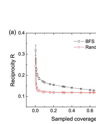
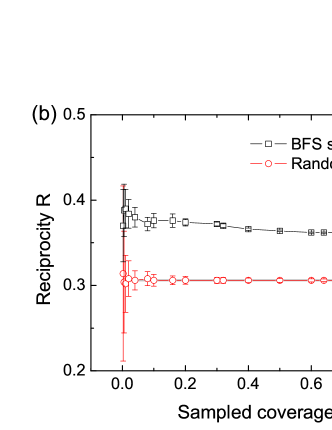
Figure 7: (Color online) Reciprocity changes as sampled coverage increases for Wiki2007 (a) and Google (b) data. Except for an initial state that results from the presence of self-links, random sampling shows constant reciprocity while BFS sampling approaches the true value slowly from above. The gray lines behind the random sampling data are the theoretical prediction for random sampling.

For random sampling, in the absence of self-links (i.e. links that start and end on the same node), reciprocity is constant, independent of sampling coverage, since any pair of nodes is chosen with the same probability as any other pair of nodes. If, however, self-links are present, the reciprocity under random sampling is higher than that of the true network since the self-links (which are reciprocal by definition) appear with probability $\alpha>\alpha^{2}$. The reciprocity with respect to $\alpha$ is $R(\alpha)\approx R(1+\alpha^{-1}c/L_{\leftrightarrow})$, where $c/L_{\leftrightarrow}$ is the fraction of self-links among bidirectional links. Thus, one can see that in the presence of self-links, the reciprocity is no longer constant, but quickly approaches its asymptotic value as ${\alpha}$ increases. The data in Fig. 7(a) illustrate this effect for Wiki2007 which exhibits a small fraction ($<0.4\%$) of self-links among all bidirectional links. The gray lines in the figures are the expectation lines from the above equation and agree perfectly with the data.

For BFS sampling, however, reciprocity is significantly overestimated, and only slowly approaches its true value. At least part of the bias for reciprocity under BFS comes from the fact that we only include links in the growing front if they point back to the previously sampled graph. This introduces a bias to increase reciprocity. This type of overestimation is actually present at any sampling coverage for an additional reason: BFS sampling (in most cases) only gathers information about the GSCC and OUT components, but not about the IN and other components, and since reciprocal links always tie two nodes into one component, there are naturally more reciprocal links in the GSCC than there are in other components as summarized in Table 3; thus there is overrepresentation of bidirectional links, relative to the total number of links, and reciprocity is artificially high as shown most clearly in Fig. 7(b) for the Google data.

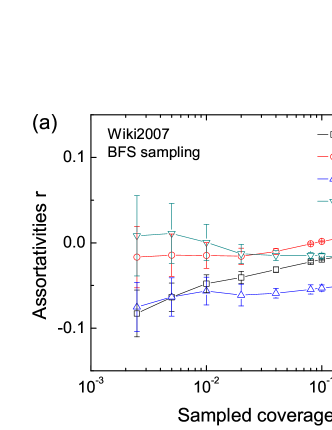
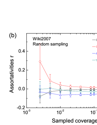
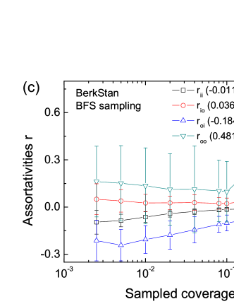
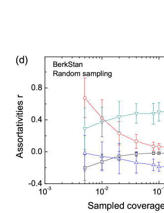
Figure 8: (Color online) Four kinds of assortativity for BFS-sampled networks and random-sampled ones on (a), (b) Wiki2007 data and (c), (d) BerkStan data.

III.4 Assortativities

A set of assortativity measures JFoster2010 for directed networks are defined using the Pearson correlation as follows:

$$r_{xy}=\frac{L^{-1}\sum\limits_{l\in\mathbb{E}}\left[(j_{x}^{l}-\overline{j}_{x})(k_{y}^{l}-\overline{k}_{y})\right]}{s^{(j)}_{x}s^{(k)}_{y}},$$ (5)

where $x,y\in\{{\rm in},{\rm out}\}$ indexes each incoming and outgoing degree type and $j_{x}^{l}$ ($k_{y}^{l}$) is the $x$-degree ($y$-degree) of the tail (head) node for a link $l$, and $\mathbb{E}$ is the set of sampled links (all links, if we consider the complete network). $\overline{j}_{x}=L^{-1}\sum_{l\in\mathbb{E}}j_{x}^{l}$ ($\overline{k}_{y}=L^{-1}\sum_{l\in\mathbb{E}}k_{y}^{l}$) is the weighted average degree note1 . The following relations hold in general: $\overline{j}_{\rm out}\neq\overline{j}_{\rm in}=\overline{k}_{\rm out}\neq\overline{k}_{\rm in}$. $s^{(j)}_{x}=\sqrt{L^{-1}\sum_{l\in\mathbb{E}}(j_{x}^{l}-\overline{j}_{x})^{2}}$ is the standard deviation of the $x$-degree of the tail nodes ($\neq\sigma^{\prime}_{x}$). $s^{(k)}_{y}$ is similarly defined. It is worth noting that $s^{(j)}_{\rm in}\neq s^{(j)}_{\rm out}\neq s^{(k)}_{\rm in}\neq s^{(k)}_{\rm out}$.

In most cases, we find that the directed assortativities of the networks we study are not markedly different from zero, and it is therefore difficult to define a general tendency for the effects of BFS sampling on the statistics of assortativity. We do, however, point out that both $r_{\rm oo}$ and $r_{\rm oi}$ of the BerkStan network are quite large (but have opposite sign), suggesting that, unlike the rest of the networks, nodes of high out-degree tend to link to other nodes of high out-degree, but nodes of high out-degree tend to link with nodes of low in-degree.

While the small assortativities of the networks make it dangerous to draw broad conclusions regarding the effects of sampling, it is clear that in the case of random sampling there is a clear tendency in behavior at low values of the sampling coverage, which seems to be related to the small reciprocity of the networks we study ZamoraLopez2008 . Assortativity between the incoming degree and outgoing degree $r_{\rm io}$ tends to be overestimated for small sampling coverage; on the other hand, the incoming-incoming degree assortativity is underestimated (implying greater disassortativity than is present in the complete networks) as shown in Figs. 8(b) and (d). These trends seem to stem from a trivial situation: when the sampling coverage is small, many tail (head) nodes will have no incoming (outgoing) degree, even though they are connected to each other. Consider two nodes, A and B, connected by a directed link from A to B. In this case, A has no incoming degree and B has no outgoing degree. Thus the correlation between in- and out-degrees would be positive, whereas the correlation between incoming degrees would be negative. This would not be the case if a large fraction of nodes had reciprocal links. Not surprisingly, these tendencies disappear very quickly as the sampling coverage increases.

Assortativity can be either overestimated or underestimated by BFS, depending on network structure and coverage. The real value of in-degree/in-degree assortativity is approached from below in Wikipedia data (see Fig. 8(a)). When randomly picking the seeds for BFS, there is a high chance to select small $k^{i}_{\rm in}$ nodes since incoming degree follows a scale-free distribution. Nonetheless, BFS sampling soon reaches the large $k^{i}_{\rm in}$ nodes. This results in a highly negative $r_{\rm ii}$ initially. As the sampling coverage increases, $r_{\rm ii}$ approaches its real value from below. However, we do not observe systematic behaviors for other assortativities under BFS.

III.5 Number of SCCs

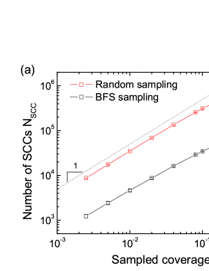
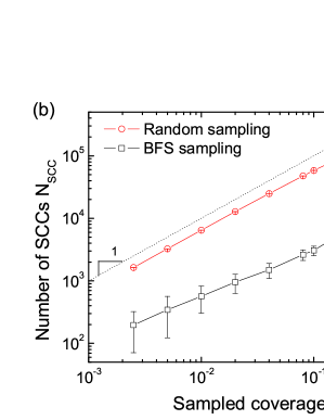
Figure 9: (Color online) Tendency for the number of SCCs in Wiki2007 (a) and BerkStan (b) data to increase with both sampling methods. After a threshold sampling coverage has been reached, the number of SCCs will decrease, since the newly-sampled nodes will bridge preexisting SCCs. The black dotted lines in (a) and (b) are the reference for the slope 1.

As the sampling coverage increases, the number of SCCs increases initially. Since single nodes and nodes with only incoming links are considered SCCs by definition, the number of SCCs is proportional to the sampling coverage $\alpha$, both for random and BFS sampling. However, after a certain sampling coverage has been reached, newly-sampled nodes are more likely to connect to already-existing SCCs. For most networks, this means that existing SCCs will merge together, whence the total number of SCCs will finally decrease. This is illustrated in Fig. 9. For both sampling methods, the number of SCCs increases linearly with $\alpha$ initially and then decreases to the value in the original networks for large $\alpha$. However, the number of SCCs observed in BFS sampling is almost one order of magnitude less.

III.6 Surface Nodes

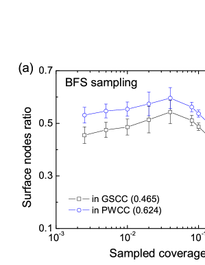
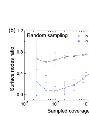
Figure 10: (Color online) Ratio of the surface nodes in the GSCC and the PWCC of (a) BFS-sampled and (b) randomly sampled networks of Wiki2007 data. In the case of the BFS sampling, the estimated values do not approach to the true values since BFS sampling only covers the all nodes in GSCC and OUT components.

Since surface nodes are in contact with other components, there is a possibility that they will be absorbed into component cores or move into other components if we add nodes or links from the network. The ratio of nodes on the surface of a component to the total number of nodes in the component (‘surface node ratio’) seems to depend strongly on the structure of the SCCs of directed networks. Of the networks we study, the Wikipedia graphs have the largest GSCCs, with upwards of 67% of all nodes, and at least 43% of theses nodes are surface nodes. The Stanford and BerkStan networks’ GSCCs are smaller (59% and 51%, respectively) and contain very few surface nodes (7.4% and 9.6%, respectively). A closer look at the IN and OUT components of the Stanford network reveals numerous chains and multinode (directed) cycles that offer only a single surface node for attachment to the GSCC. Figure 10 shows the changes to surface node ratios as sampling coverage increases in the Wiki2007 data.

When the sampling coverage is small, the surface node ratio in the GSCC does not change markedly under random sampling. After increasing the sampling coverage, however, the ratio decreases as the core becomes more densely connected with the addition of newly sampled nodes. However, the surface node ratio in the PWCC increases as shown in Fig. 10(b) as the DISC and TEND shrink quickly, becoming absorbed into the GSCC, and then transforming into surface nodes.

BFS sampling, on the other hand, shows a different trend. The surface node ratio in the GSCC is lower than that in the PWCC. This seems to be deeply related with the fact that BFS sampling starts from seeds than expands their territory layer by layer. When the sampling coverage is small, the surface node ratio increases as the sampling coverage increases. After the sampling procedure has reached a certain point, the surface node ratio will also begin to decrease as shown in Fig. 10(a).

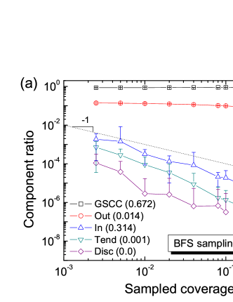
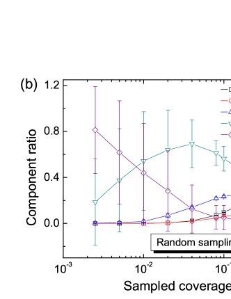
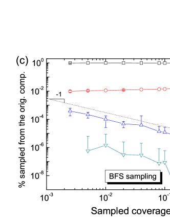
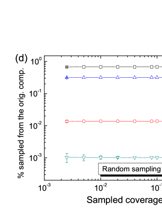
Figure 11: (Color online) For Wiki2007 data, component ratios in the sampled networks (a), (b), and percentages sampled from the components in the original network (c), (d). (a) It is surprising that most of the network is a GSCC even at very low coverage, indicating the importance of loops and clustering around high in-degree nodes. The OUT component ratio slightly decreases as $\alpha$ increases since the number of nodes in the GSCC increases more quickly than the number of nodes in the OUT. (c) Conversely, the percentage sampled from the OUT increases. As expected, the other components shrink as a power of $1/N\approx\alpha^{-1}$. (d) In the case of random sampling, the percentage sampled from each component is almost constant. (b) On the other hand, the component ratio changes substantially as the sampled coverage increases. At small coverage, most of the nodes are disconnected, but after a percolation threshold has been reached, the GSCC emerges quickly, absorbing the other components. The labels for (c), (d) are the same as those of (a), (b) and the numbers in parentheses are the component ratio of the original network.

III.7 Components Ratios

Here we focus both on the evolution of the bow-tie structure and on the component from which the nodes are sampled – noted in Fig. 11(c) and (d) as “% sampled from the orig. comp.”– as the sampling coverage increases. BFS sampling mainly covers the GSCC and OUT components, so the sizes of the IN and TEND components in the sampled networks remain constant as $\alpha$ increases. As coverage increases, the size ratio of the GSCC – the ratio of nodes in the current GSCC to the total number of discovered nodes – increases slightly as the GSCC absorbs other components.

The main characteristics associated with random sampling are described by percolation phenomena Albert2000 ; Cohen2000 ; Cohen2001 . When the sampling coverage is small, most of the nodes are disconnected and belong to the DISC and TEND components. As sampling coverage increases past some percolation threshold, the GSCC emerges quickly and the IN and OUT components form concurrently as shown in Fig. 11(b).

IV Summary and Discussion

In summary, a comparison of BFS sampling to random sampling indicates that differences in sampling method and coverage can introduce biases that result in substantial mischaracterization of the statistics of many structural properties in directed networks. Moreover, the extent to which sampling biases will affect these properties seems to depend heavily on the structure of the original network. In comparing random sampling to BFS sampling on seven different directed networks, including three versions of Wikipedia, three different sources of sampled World Wide Web data, and an Internet-based social network, we found that differences in sampling method and coverage affect both the bow-tie structure, as well as the number and surface structure of strongly connected components in sampled networks. In addition, at low sampling coverage (less than 40%), the values of average degree, variance of in- and out-degree, degree auto-correlation, and link reciprocity in sampled networks are misestimated by at least 30%, and sometimes by as much as four orders of magnitude. The structural properties of BFS-sampled networks attain values within 10% of the corresponding values in the original networks only when sampling coverage is in excess of 65%.

Most biases under random sampling seem to stem from the fact that both out-degree and in-degree will be approximately equally undersampled. This leads to underestimation of average degree and variances of in- and out-degree. At the same time, properties such as reciprocity and auto-correlation are essentially constant because of this equality in undersampling. Biases under BFS sampling arise from a confluence of factors: by following only outgoing links, BFS fails to cover the IN-component of directed networks; BFS covers nodes of high in-degree at early times; the core of BFS-sampled networks are tangled with many loops showing high clustering; the in- and out-degrees of nodes at the growing front are undersampled under BFS sampling. In combination, these factors (and, possibly others) lead to overestimation of some structural properties (average degree, variance in out-degree, auto-correlation, and reciprocity) and underestimation of others (variance in in-degree, number of SCCs, surface node ratios). We have demonstrated that for these reasons, if uniform random, or BFS sampling is used to assemble a network, significant corrections to degree, degree variance, auto-correlation, reciprocity, some types of assortativity and component make-up should be expected.

Though we have not examined it here, we suspect that there may be an important interplay between sampling method, sampling coverage, temporal changes, and sampled network topologies. The Wikipedia data discussed earlier could be used to probe such effects, since it captures snapshots of Wikipedia at different times during the network’s evolution. It would be interesting to quantify differences in the effects (if any) of BFS and random sampling on time-varying or temporal networks Holme2012 . A natural question, after analyzing the drawbacks of sampling procedures, will be how we can overcome such problems to get unbiased network samplings. A possible solution could be a combination of random and BFS samplings to get several unbiased structural properties. However, it is still challenging work to get unbiased samplings for every network properties. There are several papers suggesting unbiased sampling strategies for specific properties Kurant2010 ; Kurant2011 .

The results presented in this paper have widespread implications for conclusions that have been drawn regarding the structure (and function) of some of the most ubiquitously studied real-world networks, including the World Wide Web. Since for many studied real, directed networks only an incomplete link list is available, either because the networks are too large to be fully recorded, or because they change too quickly to be captured by any sampling procedure, our findings call into question the accuracy of previous, reported results for the statistics of some of these networks’ structural properties. We may not know as much about the structure of very large directed networks as has been supposed.