One method for constructing exact solutions of equations of two-dimensional hydrodynamics of an incompressible fluid

Abstract

We propose a simple algebraic method for constructing exact solutions of equations of two-dimensional hydrodynamics of an incompressible fluid. The problem reduces to consecutively solving three linear partial differential equations for a nonviscous fluid and to solving three linear partial differential equations and one first-order ordinary differential equation for a viscous fluid.

I Introduction

The dynamics of incompressible viscous fluid flows is described by the Navier-Stokes (NS) equation. In the regime of large Reynolds numbers (Re), turbulence arises, presenting one of the most important unsolved problems in theoretical and mathematical physics. Formally, letting Re tend to infinity (or the viscosity tend to zero), we obtain the Euler equations. Whose mathematical analysis is still more difficult than the investigation of the NS equation. And the NS equations themselves can be regarded at large values of ${\rm Re}$ as singularly perturbed Euler equations.The results by Kato show that the two-dimensional NS equations are globally defined in $C^{0}\left([0,\infty];\,H^{s}(R^{2})\right)$, and that for $s>2$ and $0<T<\infty$ the ”weak solution” of the two-dimensional NS equations tends to the solution of the two-dimensional Euler equation in $C^{0}\left([0,T];\,H^{s}(R^{2})\right)$ Kato . In turn, the three-dimensional NS equation is locally defined in $C^{0}\left([0,\tau];\,H^{s}(R^{2})\right)$, and for $s>5/2$ its ” weak solutions” are approximated by solutions of the three-dimensional Euler equations in $C^{0}\left([0,\tau];\,H^{s}(R^{3})\right)$ when $\tau$ is determined by the initial data (by the norm) and by the external forces Kato1 , Kato2 . The nonviscous limit was intensively studied in Constantin , Wu . The mathematical investigation of the NS and Euler equations is undoubtedly one of the most important problems of mathematical physics. The are now enormously many publications devoted to various aspects of these equations. Among the most important results, we can mention thee proof of the Hamiltonian character of the two-dimensional Euler equations by Arnold Arnold and the investigation results on the symplectic structure of these equations Marsden . In Friedlander1 and Friedlander2 the Lax representation was found for the two-dimensional Euler equation written in the Euler variables. The Lax representation was later also constructed in the Euclidean variables 2525 .

In this paper, we describe an astonishingly simple, but effective, method for constructing exact solutions of equations of two-dimensional hydrodynamics of an incompressible fluid. This method is applicable to both nonviscous and viscous fluids (accordingly, to the Euler and NS equations). The paper has the following structure. In Sec.2, we demonstrate this method for the two-dimensional Euler equations describing nonviscous incompressible fluid flows. We give some examples of exact solutions in Sec.3. In Sec.4, we generalize the above mentioned method to the case of viscous two-dimensional flows. We summarize the presented results in Sec.5.

II Two-dimensional Euler equations

We consider the flow of a nonviscous incompressible two-dimensional fluid. The two velocity components $v_{x}$ and $v_{y}$ are expressed in terms of the stream function $\psi=\psi(t,x,y)$

$$v_{x}=\frac{\partial\psi}{\partial y},\qquad v_{y}=-\frac{\partial\psi}{\partial x},$$ (1)

as a result of which the continuity equation ${\rm div}{\vec{v}}=0$. In these variables, the two-dimensional Euler equation assumes the form Landau :

$$\frac{\partial\triangle\psi}{\partial t}+\frac{\partial\psi}{\partial y}\frac{\partial\triangle\psi}{\partial x}-\frac{\partial\psi}{\partial x}\frac{\partial\triangle\psi}{\partial y}=0,$$ (2)

where $\triangle$ is the two-dimensional Laplacian.

Equation (2) is a nonlinear equation that is not one of the so-called integrable equations (despite the existence of the Lax representation). Nevertheless,it is possible to develop a procedure for constructing exact solutions for it. More precisely,there exist transformations that allow finding exact solutions of Eq. (2) that describe nonpotential (i.e.,eddying) fluid flows proceeding from solutions describing potential flows. the crux of the matter is expressed by the following theorem.

Theorem 1. Let $\psi(x,y)$ be a harmonic function in a domain $D$, i.e., $\triangle\psi=0$ where $\triangle$ is the two-dimensional Laplacian. Let $F(t,x,y)$ be a solution of the overdetermined system of linear differential equations

$$\begin{array}[]{cc}\displaystyle{\triangle F=kF},\\ \\ \displaystyle{\frac{\partial F}{\partial t}=\frac{\partial\psi}{\partial x}\frac{\partial F}{\partial y}-\frac{\partial\psi}{\partial y}\frac{\partial F}{\partial x}-\frac{d\ln k}{dt}F},\end{array}$$ (3)

where $k(t)$ is a function of time. Then the function

$$\psi_{1}=\psi+F,$$ (4)

satisfies in $D$ Eq. (2), i.e.

$$\frac{\partial\triangle\psi_{1}}{\partial t}+\frac{\partial\psi_{1}}{\partial y}\frac{\partial\triangle\psi_{1}}{\partial x}-\frac{\partial\psi_{1}}{\partial x}\frac{\partial\triangle\psi_{1}}{\partial y}=0.$$

The theorem is proved by direct calculation. In what follows, formulas (3) and (4) are called the ”dressing” procedure for the $D=2$ Euler equations.
Remark 1. The harmonic function $\psi$ is regarded as being dependent on two variables,i.e. $\psi=\psi(x,y)$. But it can also be assumed to depend on $t$ as a parameter. It can be easily verified that the theorem also holds in this case.
Remark 2. Transformation (4) resembles the Darboux transformation (DT) used in the theory of integrable systems BLP . Indeed,the essence of the DT consists in determining a solution $\Psi$ for the Lax pair with a given ”incipient” potential (which in turn is a solution of the nonlinear equation under investigation) and subsequently using $\Psi$ to find new potentials.

The similarity between the DT and the transformation described above is obvious. Indeed, as an intermediate step, we must solve two linear equations (3) with variable coefficient depending on the harmonic function $\psi$, which can be regarded as an ”incipient” potential because it satisfies Eq.(2) and describes a plane potential flow (this is a stationary flow if $\psi$ is independent of $t$). In this case, the new stream function $\psi_{1}$ in (4) describes a nonstationary eddying flow of fluid. Nevertheless, this is not a Darboux transformation, because nonlinear system (3) is not a $[L,A]$ pair for Euler equation (2). The compatibility condition for Eqs. (3) has the form

$$\triangle\theta-k\theta=\frac{dk}{dt}F,$$ (5)

where

$$\theta=\frac{\partial\psi}{\partial x}\frac{\partial F}{\partial y}-\frac{\partial\psi}{\partial y}\frac{\partial F}{\partial x}.$$

Using Eqs. (3) and the fact that $\psi$ is a harmonic function,we can rewrite Eq. (5) in a different form,

$$\left(\frac{\partial^{2}\psi}{\partial x^{2}}-\frac{\partial^{2}\psi}{\partial y^{2}}\right)\frac{\partial^{2}F}{\partial x\partial y}+\left(\frac{\partial^{2}F}{\partial y^{2}}-\frac{\partial^{2}F}{\partial x^{2}}\right)\frac{\partial^{2}\psi}{\partial x\partial y}=\frac{1}{2}\frac{dk}{dt}F.$$ (6)

But system (3) should not regarded as the Lax pair for Eqs. (5) or (6). The point is that a pair of linear equations can be regarded as a Lax pair only if their compatibility condition has the form of a nonlinear equation for the potentials.In other words, the ”wave function”(whose role in the case under consideration would be played by the function $F$), which is merely an auxiliary expression, must not enter the compatibility condition. The situation we deal with is quite different because $F$ is contained in Eq.(6). Of course, we can take a next step in finding the compatibility condition for Eqs. (6) and (3), although no elimination of the function $F$ is possible even then.We do not discuss the interesting equation of whether this procedure can be stopped after only finitely many equations are written.
Remark 3. System (3) involves an auxiliary time function $k=k(t)$. Its expression is not fixed but is determined by the form of the harmonic function $\psi$. In particular, is not compatible for all harmonic functions $\psi$ system (3) i.e., for an arbitrary function $\psi$, there can be no function $k(t)$ such that system (3) has a solution.

We show that this elementary approach unexpectedly turns out to be rather effective for constructing exact solutions of the two-dimensional Euler equation.

III Examples of exact solutions of the Euler equation

Wi consider a harmonic function of the form $\psi_{{}_{N}}=X_{{}_{N}}A_{{}_{N}}Y_{{}_{N}}$ where

$$X_{{}_{N}}=\left(\begin{array}[]{ccccc}1&x&x^{2}&...&x^{N}\end{array}\right),\qquad Y_{{}_{N}}=\left(\begin{array}[]{cccc}1\\ y\\ y^{2}\\ \vdots\\ y^{N}\end{array}\right),$$ (7)

$A_{{}_{N}}$ is a constant $(N+1)\times(N+1)$ matrix with elements $a_{ik}$, and $i$ and $k$ range from zero to $N$. The expression for the matrix $A_{{}_{N}}$ is found by substituting $\psi_{{}_{N}}$ in the equation $\triangle\psi_{{}_{N}}=0$. We present several examples for different values of $N$:

$$A_{1}=\left(\begin{array}[]{cc}a_{00}&a_{01}\\ a_{10}&a_{11}\end{array}\right),\qquad A_{2}=\left(\begin{array}[]{ccc}a_{00}&a_{01}&a_{02}\\ a_{10}&a_{11}&0\\ -a_{02}&0&0\end{array}\right),$$

$$A_{3}=\left(\begin{array}[]{cccc}a_{00}&a_{01}&a_{02}&a_{03}\\ a_{10}&a_{11}&-3a_{30}&a_{13}\\ -a_{02}&-3a_{03}&0&0\\ a_{30}&-a_{13}&0&0\end{array}\right),\qquad A_{4}=\left(\begin{array}[]{ccccc}a_{00}&a_{01}&a_{02}&a_{03}&a_{04}\\ a_{10}&a_{11}&-3a_{30}&a_{13}&0\\ -a_{02}&-3a_{03}&-6a_{04}&0&0\\ a_{30}&-a_{13}&0&0&0\\ a_{04}&0&0&0&0\end{array}\right),$$

$$A_{5}=\left(\begin{array}[]{cccccc}a_{00}&a_{01}&a_{02}&a_{03}&a_{04}&a_{05}\\ a_{10}&a_{11}&-3a_{30}&a_{13}&5a_{50}&-\frac{3a_{33}}{10}\\ -a_{02}&-3a_{03}&-6a_{04}&-10a_{05}&0&0\\ a_{30}&-a_{13}&-10a_{50}&a_{33}&0&0\\ a_{04}&5a_{05}&0&0&0&0\\ a_{50}&-\frac{3a_{33}}{10}&0&0&0&0\end{array}\right),$$

etc. The number $M(N)$ of free parameters(i.e.,the number of independent elements in the matrices $A_{{}_{N}}$) is determined as follows: if $N$ is odd,then $M(N)=2(N+1)$, and if $N$ is even,then $M(N)=2N+1$. Because the stream function serves only as an auxiliary means for calculating the velocity field and vanishes under differentiation with respect to the spatial variables $a_{00}$,we can set $a_{00}=0$ without loss of generality, which is precisely implied in what follows. The other entries should be regarded as functions of time, i.e., $a_{ij}=a_{ij}(t)$. Substituting $\psi_{{}_{N}}$ in system (3) and solving it, we extract the function $F$, after which the corresponding function $\psi_{1,{{}_{N}}}$ is calculated using formula (4).

We demonstrate this approach for some specific examples. Let $N=1$. In this case, $a_{11}=0$ should be chosen.It is convenient to parameterize $a{01}(t)$ and $a_{10}(t)$ as

$$a_{01}(t)=A(t)\sin\alpha(t),\qquad a_{10}(t)=A(t)\cos\alpha(t),$$

where $\alpha(t)$ and $A(t)$ are arbitrary real functions. After a simple calculation, we finally obtain

$$\psi_{1}=A(t)\left(y\sin\alpha(t)+x\cos\alpha(t)\right)+\sum_{i=1}^{n}\left(c_{i}\sin g_{i}+c^{\prime}_{i}\cos g_{i}\right),$$ (8)

where $g_{i}=x\cos\phi_{i}+y\sin\phi_{i}+f_{i}(t)$, $\phi_{i}$, $c_{i}$, and $c^{\prime}_{i}$ are arbitrary constants, and $f_{i}(t)$ is given by the integral formula

$$f_{i}(t)=f_{i}(0)+\int dtA(t)\sin\left(\phi_{i}-\alpha(t)\right).$$

In this case, $k$ is simply a negative constant , which is set to minus unity without loss of generality. Expression (8) can be straightforwardly substituted in (2) to to ensure that we have obtained a solution of the Euler equation parameterized by two arbitrary functions $A(t)$ and $\alpha(t)$. we take $n=1$, $A(t)=\mu/\cosh^{2}\nu t$, $\alpha={\rm const}$, $c^{\prime}_{1}=0$, $c_{1}=c$, $\phi_{1}=\phi$, and $f_{1}(0)=0$. In this special case, the solution takes the form

$$\psi_{1}=\frac{\mu}{\cosh^{2}\nu t}\left(y\sin\alpha+x\cos\alpha\right)+c\sin\left[\kappa\left(x\cos\phi+y\sin\phi+\frac{\mu}{\nu}\sin(\phi-\alpha)\tanh\nu t\right)\right],$$ (9)

where $\kappa=\sqrt{-k}$, $k<0$ is introduced. Figure 1-3 shows the velocity fields for the corresponding flow at the instants $t=0$, $t=1$, and $t=50$.Here, $\alpha=0$, $\phi=\pi/4$, and the other (dimensional) parameters are set to unity.

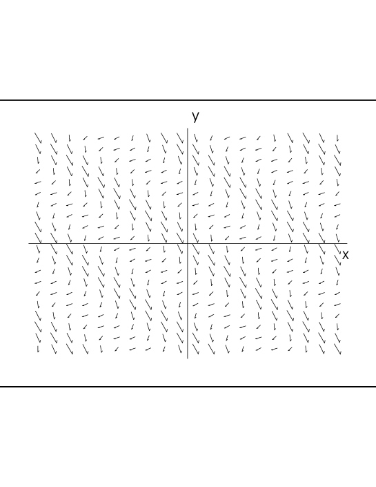
Figure 1: Graph of the velocity field for $N=1$, at the instants $t=0$ in the domain $-10<x,y<10$.

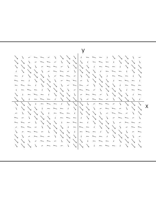
Figure 2: Graph of the velocity field for $N=1$, at the instants $t=1$ in the domain $-10<x,y<10$.

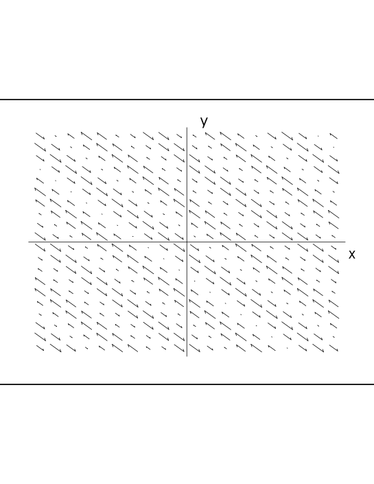
Figure 3: Graph of the velocity field for $N=1$, at the instants $t=50$ in the domain $-10<x,y<10$.

The resulting solution qualitatively resembles the so-called ”exulton”, a specific solution of the nonlinear Schrodinger equation Exul . An exulton is a rational perturbution that appears on the background of a pereodic wave, increases, and then rapidly disappears . Solution (9) behaves similarly, namely, at negative times sufficiently large in absolute value, the flow looks qualitatively the same as Fig.3. As $t$ aspiring to zero at the left, the first term in solution (9)begins to dominate, which distorts this pattern. The maximum distortion occurs at $t=0$ (see Fig. 1).After that, the first term disappears (9) exponentially fast, and we again have original (although somewhat displaced) pattern shown in Fig. 3.

We now consider the case $N=2$. Assuming that $a_{01}$, $a_{10}$, $a_{11}$ and $a_{02}$ are function of time, we seek $F$ in the form $F=\xi(t)\sin(a(t)x+b(t)y+c(t))$. Solving Eqs. (3) and using function (4) we obtain

$$\psi_{1}=a_{02}(t)\left(y^{2}-x^{2}\right)+a_{11}(t)xy+a_{01}(t)y+a_{10}(t)x+\frac{\xi_{0}\sin(a(t)x+b(t)y+c(t))}{a^{2}(t)+b^{2}(t)},$$ (10)

where $\xi_{0}$=const, and the functions $a(t)$, $b(t)$ and $c(t)$ are found from system of ordinary differential equations

$$\begin{array}[]{l}\displaystyle{\frac{da(t)}{dt}=-a_{11}(t)a(t)-2a_{02}(t)b(t),\qquad\frac{db(t)}{dt}=a_{11}(t)b(t)-2a_{02}(t)a(t)},\\ \\ \displaystyle{\frac{dc(t)}{dt}=-a_{01}(t)a(t)+a_{10}(t)b(t)}.\end{array}$$ (11)

The functions $a_{ij}(t)$ can now be chosen arbitrarily. At the next step,we substitute them in system (11) and solve it for $a(t)$, $b(t)$, and $c(t)$. Finally, substituting the resulting functions in (10) we obtain the desired solution.

As a simple example, we set $a_{11}=$const and $a_{02}$=const. Calculating as described above, we find

$$a(t)=a_{0}\cosh\omega t,\qquad b(t)=-\frac{a_{0}}{2a_{02}}\left(a_{11}\cosh\omega t+\omega\sinh\omega t\right),$$

where $a_{0}$ is the integration constant and $\omega=\sqrt{a_{11}^{2}+4a_{02}^{2}}$. For $c(t)$, it is convenient to set $a_{10}(t)b(t)=a_{01}(t)a(t)$, which gives $c$=const and we can choose $c=0$ without loss of generality. We note that solution (10) is not singular, and we have $k(t)=-a^{2}(t)-b^{2}(t)$.

The behavior of the velocity field at $t=0$ and $t=50$ is shown in Fig. 4, 5, where we have $a_{10}=a_{01}=0$, and all the other parameters are set to zero.

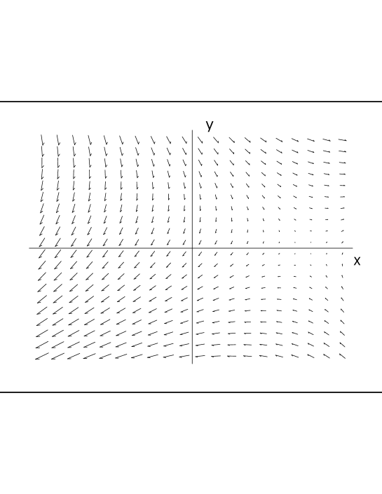
Figure 4: Graph of the velocity field for $N=2$, at the instants $t=0$ in the domain $-0.5<x,y<0.5$.

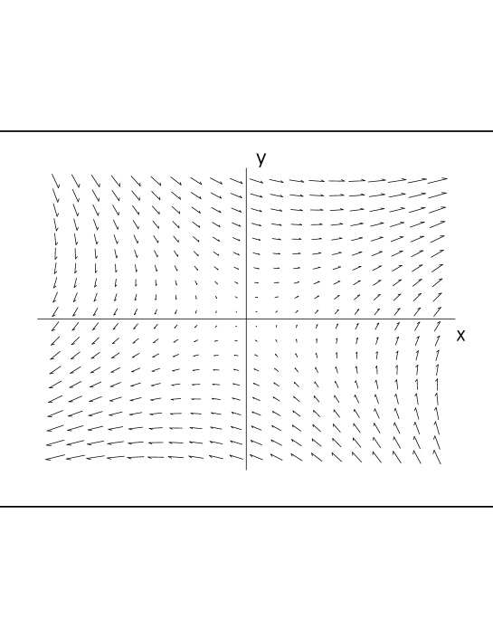
Figure 5: Graph of the velocity field for $N=2$, at the instants $t=50$ in the domain $-0.5<x,y<0.5$.

We note that in contrast to the previos solution, at times $t$ with a large absolute value, the first term dominates instead of the second. Furthermore, for large values of $x$ and $y$, the first term in expression (10) also dominates. Because the distortion of the structure occurs only in the neighborhood of the origin as $t\to 0$, the small spatial domain $-0.5<x,y<0.5$. is taken in Fig.2; the indicated changes would not be noticeable at the scales chosen in Fig.1.

Finally, we note that the same method can also be used to construct solution describing potential flows. For example, taking $N=3$ and $k=0$, we can obtain the solution of the Euler equation

$$\begin{array}[]{cc}\displaystyle{\psi_{1}=a_{01}y+a_{02}y^{2}+a_{03}y^{3}+a_{10}x+a_{11}xy-3a_{30}xy^{2}+a_{13}xy^{3}-a_{02}x^{2}-3a_{03}x^{2}y+}\\ \\ \displaystyle{+a_{30}x^{3}-a_{13}x^{3}y+{\rm e}^{ax+by+c}\left(A\sin(bx-ay-{\tilde{c}})+B\cos(bx-ay-{\tilde{c}})\right),}\end{array}$$

where all coefficients except $A$ and $B$ are arbitrary functions of time.It can be easily shown that $\triangle\psi_{1}=0$. Of course, two-dimensional potential flows can be described using the powerful method based on introducing a complex potential Landau , and using the technique described above therefore seems inconvenient in this case. The advantages of our approach for constructing exact solutions in the case of two-dimensional Euler equations become obvious only when applied to nonstationary eddying flows of fluid.

IV Two-dimensional flow of an incompressible viscous fluid

However astonishing, the technique described above can be easily generalized to the case of a two-dimensional flow of an incompressible viscous fluid described by the equations

$$\frac{\partial\triangle\psi}{\partial t}+\frac{\partial\psi}{\partial y}\frac{\partial\triangle\psi}{\partial x}-\frac{\partial\psi}{\partial x}\frac{\partial\triangle\psi}{\partial y}=\nu\triangle^{2}\psi,$$ (12)

where $\nu$ is the kinematic viscosity. Namely, the following theorem holds.

Theorem 2. Let $\psi$ be a harmonic function in a domain $D$, i.e., $\triangle\psi=0$. Let $F(t,x,y)$ be a solution of the overdetermined system of linear differential equations

$$\begin{array}[]{cc}\displaystyle{\triangle F=u(t)F},\\ \\ \displaystyle{\frac{\partial F}{\partial t}=\frac{\partial\psi}{\partial x}\frac{\partial F}{\partial y}-\frac{\partial\psi}{\partial y}\frac{\partial F}{\partial x}+U(u)F},\end{array}$$ (13)

where $u(t)$ satisfies the ordinary differential equation

$$\frac{du(t)}{dt}+uU(u)=\nu u^{2},$$ (14)

and $U(u)$ is an arbitrary function of the argument. Then the function $\psi_{1}=\psi+F$ in $D$ satisfies Eq. (12):

$$\frac{\partial\triangle\psi_{1}}{\partial t}+\frac{\partial\psi_{1}}{\partial y}\frac{\partial\triangle\psi_{1}}{\partial x}-\frac{\partial\psi_{1}}{\partial x}\frac{\partial\triangle\psi_{1}}{\partial y}=\nu\triangle^{2}\psi_{1}.$$

As in the case of Theorem 2, Theorem 1 is proved by a straightforward calculation.

As the simplest example, we consider the ”dressing” on the zero background, i.e.,$\psi=0$. we choose $U(u)=\nu u$. As follows from Eq. (14), expression $u$ is a constant. Solving system (13), we obtain

$${\psi_{1}=K{\rm e}^{-\nu\left(a^{2}+b^{2}\right)t}\left(C_{1}\sin(ax+by)+C_{2}\cos(ax+by)\right)},$$

where $K$, $a$, $b$, and $C_{1,2}$ are arbitrary constants. Of course,this simple and well-known solution, which we present here only to demonstrate the workability of the method.

We now consider case $N=1$. By analogy with expression (8), we can construct a solution of Eq. (12) in the form

$$\psi_{1}=A(t)\left(y\sin\alpha(t)+x\cos\alpha(t)\right)+\xi_{1}(t)\sin g+\xi_{2}(t)\cos g,$$ (15)

where

$$g=R\left(x\cos\phi+y\sin\phi+f(t)\right),\qquad U(u)=\nu u,\qquad u=-R^{2}={\rm const},$$

$A(t)$, $\alpha(t)$, and $f(t)$ are arbitrary function, $\phi$ is an arbitrary constant, and the functions $\xi_{1}(t)$, and $\xi_{2}(t)$ are solutions of the system of ordinary differential equations

$$\begin{array}[]{c}\displaystyle{\frac{d\xi_{1}(t)}{dt}=-\nu R^{2}\xi_{1}+R\left(\frac{df(t)}{dt}-A(t)\sin(\phi-\alpha(t))\right)\xi_{2}},\\ \\ \displaystyle{\frac{d\xi_{2}(t)}{dt}=-\nu R^{2}\xi_{2}-R\left(\frac{df(t)}{dt}-A(t)\sin(\phi-\alpha(t))\right)\xi_{1}}.\end{array}$$

Of course, by analogy with expression (8), a superposition of arbitrarily many sine and cosine functions can be constructed instead of (15). This observation is a consequence of the linearity of Eqs. (13) and of the linearity of the transformed function $\psi$ in the spatial variables. In special case $df(t)/dt=A(t)\sin(\phi-\alpha(t))$, we obtain

$$\psi_{1}=A(t)\left(y\sin\alpha(t)+x\cos\alpha(t)\right)+{\rm e}^{-\nu R^{2}t}(\xi_{1}(0)\sin g+\xi_{2}(0)\cos g),$$

where $\xi_{1,2}(0)$ is the integration constant. Comparing this (8) and (9), we see that including viscosity, as should be expected, leads to an additional exponential factor descibing the dissipation.

V Conclusion

The equations of two-dimensional hydrodynamics of an incompressible fluid thus admit a simple algebraic method for constructing exact solution. Here, we confined ourself to demonstrating the simplest solution for the cases of nonviscous and viscous fluid separately. There is no doubt that the suggested technique can be used to construct many much more complicated and physically interesting solutions.

The most interesting open equation is using the ”dressing method” to solve boundary problems. For example, we consider Eqs. (13) and (14). If we solve the two equations $\triangle\psi=0$ and $\triangle F=u(t)F$ with given identical boundary conditions $S$ (it is reasonable to consider the second boundary problems,i.e.,the Neumann problem), then the solution $\psi_{1}$ obtained by the above mentioned method will satisfy the boundary conditions $2S$. On the other hand, the function $F$ must satisfy an additional dynamical equation, which may turn out to be incompatible with solution of the given boundary problem. Consequently, the equation should be stated as follows. What is the class of Neumann boundary conditions that is compatible with system (13), (14) and the equation $\triangle\psi=0$? We hope to return to this problem in our further publications.

Acknowledgments

The authors express their gratitude to the referee, whose valuable remarks and suggestions undoubtedly allowed them to improve the paper. The authors are grateful to A.K.Pogrebkov and Y.Li. One of the authors (A.V.Yu) cordially thanks the Department of Mathematics, University of Missouri-Columbia(USA), for the Miller’s Scholar position.

References

- (1) Kato T. Proc. Symp. Pure Math., Part 2, 45:1 7, (1986).
- (2) Kato T. Journal of Functional Analysis, 9:296 305 (1972)
- (3) Kato T. Quasi-Linear Equations of Evolution, with Applications to Partial Differential Equations. Lecture Notes in Mathematics, 448:25 70, (1975).
- (4) Constantin P. and Wu J. The Inviscid Limit for Non-Smooth Vortivity. Indiana University Mathematics Journal, 45, No.1, (1996).
- (5) Wu J. J. Diff. Equations, 142, No.2:413 433, (1998).
- (6) Arnold. V. I. Sur la Geometrie Differentielle des Groupes de Lie de Dimension Infinie et ses Applications a L hydrodynamique des Fluides Parfaits. Ann. Inst. Fourier, Grenoble, 16,1:319 361, (1966).
- (7) Marsden J. E. Lectures on Mechanics, Lond. Math. Soc. Lect. Note, Ser. 174. Cambridge Univ. Press, (1992).
- (8) Friedlander S. and Vishik M. Phys. Lett. A, 148, no. 6-7:313 319, (1990).
- (9) Friedlander S. and Vishik M. Nonlinearity, 6, no. 2:231 249, (1993).
- (10) Y. Li and A. Yurov. Studies In Applied Math., 111, pp. 101-113 (2003).
- (11) L.D.Lifshits, Hydrodymanics [in Russian] (Vol. 6 in Course of Theoretical Physics,3rd ed.), Nauka,Moscow (1986); English transl.prev.ed.: Fluid Mechanics, Pergamon, Oxford (1987).
- (12) A. V. Yurov, BLP dissipative structures in plane, Physics Letters A, V.262, Pages 445-452 (1999).
- (13) A.R. Its, A.V. Rybin, and M.A. Sall’, Theor.Math.Phys., 74 N1 (1988).