Interaction of Close-in Planets with the Magnetosphere of their Host Stars. II. Super-Earths as Unipolar Inductors and their Orbital Evolution

Abstract

Planets with several Earth masses and a few day orbital periods have been discovered through radial velocity and transit surveys. Regardless of their formation mechanism, an important evolution issue is the efficiency of their retention in the proximity of their host stars. If these “super-Earths” attained their present-day orbits during or shortly after the T Tauri phase of their host stars, a large fraction of these planets would have encountered intense stellar magnetic field. Since these rocky planets have a higher conductivity than the atmosphere of their host stars, the magnetic flux tube connecting them would slip though the envelope of the host stars faster than across the planets. The induced electro-motive force across the planet’s diameter leads to a potential drop which propagates along a flux tube away from the planet with an Alfven speed. The foot of the flux tube would sweep across the stellar surface and the potential drop across the field lines drives a DC current analogous to that proposed for the electro-dynamics of the Io-Jupiter system. The ohmic dissipation of this current produces potentially observable hot spots in the star envelope. It also heats the planet and leads to a torque which drives the planet’s orbit to evolve toward both circularization and a state of synchronization with the spin of the star. The net effect is the damping of the planet’s orbital eccentricity. Around slowly (or rapidly) spinning stars, this process also causes rocky planets with periods less than a few days to undergo orbital decay (or expansion/stagnation) within a few Myr. In principle, this effect can determine the retention efficiency of short-period hot Earths. We also estimate the ohmic dissipation interior to these planets and show that it can lead to severe structure evolution and potential loss of volatile material in them. However, these effects may be significantly weakened by the reconnection of the induced field.

1 Introduction

An important milestone in planetary astronomy is the discovery of a Jupiter-mass planet, 51 Peg b (Mayor and Queloz 1995, ). Its extraordinary 4 day orbital period rekindled a theoretical expectation that protoplanets may undergo orbital decay (Goldreich & Tremaine 1980, ; Lin & Papaloizou 1986, ) as a consequence of their tidal interaction with their natal disks. Today, more than 500 planets have been discovered around nearby stars. Among them, there is a pile up of $\sim$100 planets with periods ($P$) less than a week and mass ($M_{p}$) two orders of magnitude larger than that of the Earth ($M_{\oplus}$). Transit observations of some of these planets indicate that they have a radius and density comparable to that of Jupiter and Saturn and are commonly referred to as hot Jupiters.

These hot Jupiters, including 51 Peg b, were formed in presumably at some preferred locations (beyond the snow line) of their natal disks (Ida & Lin 2008, ; Ida & Lin 2010, ). After acquiring sufficient masses to open gaps in their natal disk, they undergo type II migration along with the viscous diffusion of their surrounding gas. In order to account for their survival, we proposed that the migration of 51 Peg b and other short-period gas giant planets may have stalled when they entered into the magnetospheric cavity of their host star during their infancy (Lin et al. 1996, ). Since protostellar disks are expected to be truncated within the magnetosphere of their central stars (see below), once any protoplanet enters into this region, its migration would slow to a halt as the intensity of its tidal interaction with its nascent disk weakens.

The existence of magnetosphere around T Tauri stars was proposed (Konigl 1991, ) to account for the observed period distribution which peaks around 8 days (Bouvier et al. 1993, ). If efficient angular momentum flow between protostellar disks and the magnetosphere of their central stars can enforce corotation at their interface where the magnetic and viscous torques are balanced (Shu et al. 1994, ), we would infer kilogauss fields. Today, Zeeman splitting of emission lines have been directly measured for many T Tauri stars and these observations confirm the presence of kilogauss fields on their surface (Johns-Krull 2007, ). If this field strength represents that of a dipole stellar field, the magnetospheric radius for T Tauri stars with accretion rates in the range of $10^{-8}to10^{-7}M_{\odot}$ yr^-1 would extend to regions beyond the orbits of their close-in planets. The radius of this magnetospheric cavity expands during the depletion of the disk gas and the decline of the accretion flux through the disk.

Although the magnetospheric-cavity scenario provides a useful qualitative model for the abundant population of short-period planets, a detailed reconstruction of the observed period distribution requires a quantitative determination of short-period planets’ retention efficiency. After they have entered the magnetospheric cavity of their host stars or after they have been engulfed by the magnetospheric cavity, protoplanets continue to interact with the stellar magnetic field. It is not clear whether this process can induce planets to undergo further orbital interaction.

In order to understand the nature of this physical mechanism, we carry out a series of investigations. In Paper I (Laine et al. 2008, ), we provided a general description of the relevant physical effects. We first consider the retention of short-period gas giant planets inside the stellar magnetosphere. We decompose the stellar magnetic field into a steady and a periodically modulating component and the planet into a day and night side. In this previous investigation, we considered the periodically modulating component of the field which can be due to either the planet’s eccentric orbit or the star’s non-synchronous (with respect to the planet’s orbital angular frequency) and non-aligned (with respect to the star’s magnetic poles) spin. On the night side of the planet where the magnetic diffusivity is relatively high, this time-dependent field can permeate into the planet’s envelope and induce an AC current. The ohmic dissipation of this current not only heats the planet but also provides a torque which drives the planet’s orbit toward a state of circularization and synchronization with the star’s spin. We also found that close to the host star where the stellar magnetosphere is intense, ohmic dissipation can cause a planet’s interior to heat up such that it expands and overflows its Roche lobe. The gas flow from the planet to its host star via the inner Lagrangian point also transfers angular momentum to the orbit of the planet (Gu et al. 2003, ). This process can halt the migration of the planet despite its loss of angular momentum as a consequence of its tidal interaction with the disk and the host star and the direct torque applied by the stellar magnetosphere on it. The results of this analysis will be presented elsewhere.

Another class of planets have been discovered with $M_{p}\sim$ a few $M_{\oplus}$ and $P$ in the range of a few days to 2 months. In contrast to their Jupiter-mass siblings, these planets probably have rocky or icy internal structures and are commonly referred to as super-Earths (Mayor et al. 2008, ; Howard et al. 2010, ). Recently Kepler mission led to the discovery of over 1200 planetary candidates. Since they all have radii more than twice that of the Earth, they may also be super-Earths, albeit their masses are yet to be determined. These super-Earths too are probably formed at locations ranging from a fraction to several AUs from their host stars (Ida & Lin 2008, ; Ida & Lin 2010, ). In contrast to the gas giants, super-Earths may not have adequate mass to open a gap and undergo type II migration. Nevertheless, they do tidally interact with their natal disk and undergo type I migration, due to an imbalance between the torque they exert on the disk at the Lindblad and corotation resonances both interior and exterior to their orbits (Tanaka et al. 2002, ).

In most regions of the disk, type I migration is directed inward. However, due to the corotation torque, there are migration barriers where the orbital decay of isolated super-Earths may be halted (Masset et al 2006, ; Paardekooper et al. 2010, ). These barriers occur at gas surface density ($\Sigma_{g}$) maximum near the snow line ($a_{\rm ice}$ where water vapor condensate), at the inner edge of a dead zone ($a_{\rm dead}$ where the ionization fraction near the mid plane is too small to maintain coupling between turbulent magnetic field and disk gas), and just outside the magnetospheric cavity, $a_{\rm mag}$ (Kretke & Lin 2007, ; Kretke et al. 2009, ).

Since $\Sigma_{g}$ and the mid-plane temperature of the disk decline with time, the location of these barriers also evolves with them. During the advanced stages of disk evolution, $\Sigma_{g}$ may be sufficiently small that the dead zone essentially vanishes and the stalled embryos near $a_{\rm ice}$ and $a_{\rm dead}$ resume their migration. Assuming the field strength decreases slowly or remains unchanged, the location of $a_{\rm mag}$ also expands beyond the orbital semimajor axis of the super-Earths, $a_{\rm SE}$, during the transition from classical to weak-line T Tauri phases on a timescale of $\sim 10$ Myr (Kretke & Lin 2010, ). After the disk depletion, the stellar magnetic field and spin rate decrease (Skumanich 1972, ) on a timescale $\sim 100$ Myr (Soderblom et al. 1993, ). During these evolutionary stages, the location ($a_{\rm corote}$) where the frequency of the Keplerian motion matches that of the stellar spin also evolve relative to $a_{\rm SE}$. Thus, we anticipate that some super-Earths are located interior to the corotation radius while others are located beyond it.

In this paper, we consider the interaction between close-in super-Earths with the steady component of their host stars’ magnetic field. Beside differences between their masses and radii, rocky planets have much larger electric conductivity on their surface than the envelope and atmosphere on the night side of close-in young gas giant planets. The dayside of gas giant planets is exposed to the stellar ionizing photons and may have much higher ionization fraction and electrical conductivities than their night side. We will consider this more complex aspect of the hot Jupiter problem elsewhere.

The super-Earth problem we are considering here is analogous to the Echo satellite (in the form of a conductor) moving relative to background (Earth) field line which was analyzed by Drell et al. (1965). In general, an electric field is induced across the conductor (in directions orthogonal to the field and motion). However, the electric field must vanish (in its frame) inside a perfect conductor (with an infinite conductivity). On its surface, the electric field generate a current which leads to an induced magnetic field. The induced field cancels the unperturbed field inside the conductor so that there is no relative motion between the perfect conductor and the net (unperturbed plus induced) field inside it. Outside the moving conductor, the net field appears to wrap around it. At large distances from the moving conductor, the induced field propagates away from it with the Alfven speed.

In a slightly different context, Goldreich and Lynden-Bell (1969) analyzed the electrodynamic interaction between Io and Jupiter. They treated Io as a conductor moving in Jupiter’s magnetosphere. Because Io’s conductivity is larger than that of Jupiter, it drags a flux tube of field lines. They showed that an electromagnetic field is induced across Io’s surface. Provided the conductivity is high along and low across the field lines, the electric potential drop across them would propagate and be maintained along the field lines connecting Io and Jupiter with an Alfven speed. At the foot of the flux tube where it enters into Jupiter’s atmosphere and envelope, conductivity across the field lines increases with the density of the surrounding gas such that the potential drop drives a DC current across the potential drop. Provided that the induced field can propagate back to Io before the unperturbed field slips through it, the current forms a close circuit. In this scenario, Io acts as a unipolar inductor.

In this paper, we apply the Goldreich and Lynden-Bell’s model to the study of a super-Earth moving in its host star’s magnetosphere. For computational simplicity, we neglect the planet’s intrinsic magnetic field, as we have done in the previous paper. In the problem we are considering, a steady component of the stellar magnetic field is present regardless of the differential motion between the star’s spin and the planet’s orbit. In an asynchronous system, a flux tube of magnetic field between the planet and the star cannot be infinitely anchored on both entities. If the planet’s conductivity is smaller than that on the surface of the host star, the flux tube would tend to be anchored on the surface of the star along with all other unperturbed field lines and it would slip through the planet.

In Section 2, we introduce qualitative discussion and schematic illustration to show in the limit that the electric conductivity in the super-Earth planet is higher (but not by an infinite amount) than that of its host star’s envelope, the relative motion between the planet and the stellar magnetic field leads to an induced emf and a potential drop across the planet. Outside the planet, a flux tube of (unperturbed plus induced) magnetic fields would appear to be approximately anchored on the planet. In the tenuous regions between the planet and its host star, the conductivity along the field lines is much higher than that across them and the electric current flows freely to maintain constant electric potential along them. In the absence of field reconnection, Alfven waves propagate to infinity on open lines and the electric current flows to the surface of the host stars along closed field lines. Due to the finite resistance of the surrounding (stellar) gas, the foot of the flux tube on the surface of the host star slips through the stellar atmosphere and the electrical potential drop across the foot of the flux tube drives an electric current with an associated rate of ohmic dissipation.

Based on the above qualitative scenario, we construct a quantitative model in this paper. In Section 3, we introduce the values of the different parameters we use in the numerical applications and derive the analytical expressions for the induced electric field, intensity, ohmic dissipation, and torque. In our numerical applications, we adopt a set of fiducial physical parameters for a rocky super-Earth planet with two Earth radii, $2R_{\oplus}\approx 1.4\times 10^{7}$m on a 3 day circular orbit ($a\approx 6\times 10^{9}$m around a T Tauri star with a mass equals to that of the Sun ($1M_{\odot}\approx 2\times 10^{30}$kg) and a radius twice that of the Sun $R_{\ast}=2R_{\odot}\approx 1.4\times 10^{9}$m. We also assume that it has a solar luminosity ($1L_{\odot}$), a surface temperature of $T_{\ast}=4\times 10^{3}$K, and a dipole field with a strength 0.2 T (i.e. $2\times 10^{3}$ G) on the stellar surface (which corresponds to a magnetic dipole strength of $5.4\times 10^{33}{\rm Am}^{2}$).

With these parameters, we first analyze two limiting cases of rapid and slow stellar spin. We discuss the condition of validity of the model in Section 4 and derive in Section 5 the expressions and values of the resistances and Alfven speed. We will consider more general sets of model parameters elsewhere. In Section 6, we calculate the values of the induced intensity, ohmic dissipation, and torque, and discuss the relevance of these values. In the context of planetary migration in the presence of their natal disk, we show that if the planet orbits around the host star outside its corotation radius (i.e. the Keplerian frequency of the planet’s orbit is smaller than the stellar spin frequency), the net torque associated with this induced current would provide an adequate rate of angular momentum transfer to balance against the rate of tidally induced angular momentum loss by the rocky planet to the disk. In the limit that the planet is inside its host star’s corotation radius, the planet’s orbit would continue to decay. Finally, we summarize our results and discuss their implications in Section 7.

2 Qualitative Illustration and Description of the Phenomena and Brief Outline of the Calculation

We consider a rocky planet with a mass of several $M_{\oplus}$ moving in the dipole magnetic field of the star it is orbiting. The relative motion of such a conductor in an external stellar magnetic field generates an induced emf across the planet. There are two complementary effects (see paper 1) described by the complete magnetohydrodynamic (MHD) equation: the diffusion of the magnetic field in the planet and the magnetic induction (with its associated drag).

The MHD equation describing the electrodynamics of the planet in the stellar field can be written as

$$\frac{\partial\textbf{B}}{\partial t}=\nabla\wedge\left(\upsilon\wedge\textbf{B}\right)-\nabla\wedge\left(\eta\nabla\wedge\textbf{B}\right)$$ (1)

where $\eta$ is the magnetic diffusivity (which is equal to $(\mu_{0}\sigma)^{-1}$ where $\sigma$ is the electric conductivity).

In Paper 1, we focused on the diffusion of the stellar magnetic field inside a hot Jupiter. In order to do so, we considered the periodic component of the stellar magnetic field felt by a planet when the axis of the stellar magnetic moment is not aligned with the planetary orbital axis, or when the planet is on an eccentric orbit. The drag of the magnetic field by the planet due to induction can be neglected if the planet’s orbit co-rotates with the star’s spin or if the electrical conductivity of the planet is low compared with that of the outer layers of the star (which is the case at least in the night side of a hot-Jupiter).

In this limit, the diffusion of the stellar magnetic field inside the planet is modulated by the electric conductivity (inversely proportional to the magnetic diffusivity) profile in the planet. A somewhat higher electric conductivity in the planet would tend to decrease the penetration depth of the stellar magnetic field and the volume where the electric current induced by the field can be dissipated, but it would also increase the volumic ohmic (power) dissipation rate. Likewise, a lower conductivity in the planet would enable the stellar magnetic field to penetrate deeper into it, albeit the induced current also encounters a lower volumic ohmic dissipation rate. Consequently, we found that, the total ohmic dissipation rate over the entire planet does not change significantly over a reasonable range of electric conductivity for a hot-Jupiter (neglecting the effect of photo-ionization in its atmosphere).

In the present paper, we describe the induction (and associated ”drag” of the field lines) which was neglected in paper I. For simplicity, we neglect the damping of the magnetic field in the planet associated with the diffusion term and focus on the case where the planet is able to significantly drag the stellar magnetic field lines which are enclosed in the flux tube that passes through the planet.

Throughout this paper, this ”flux tube which passes through the planet” is simply referred to as ”the flux tube” (we are interested in the part that extends between the interior of the planet and above the surface of the star). The “foot of the flux tube” refers to that part of the flux tube which extends below the surface of the star for a distance $D_{pn}$ (the subscript ”pn” refers to penetration) to be estimated below.

Between the planet and the surface of the star, the volumic current flows along the flux tube (parallel to the magnetic field lines–the electrons in fact gyrate around the magnetic field lines), but the volumic current crosses the flux tube in the planet and at the foot of the flux tube (perpendicular to the magnetic field lines in the stellar atmosphere). Figures 1 and 2 present the general overview of the system.

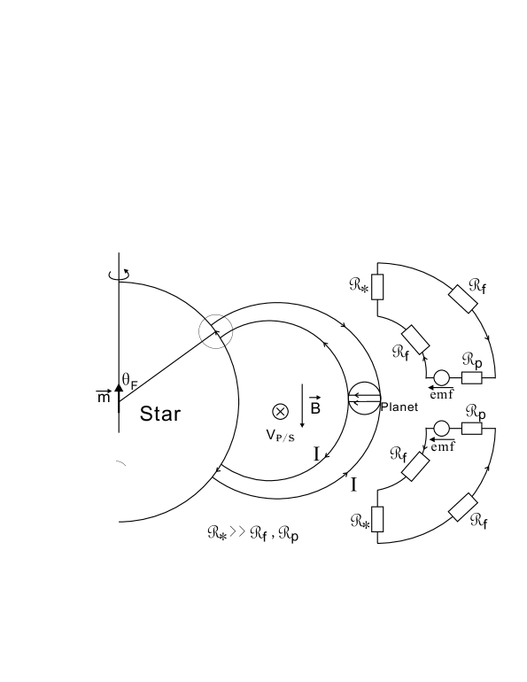
Figure 1: Schematic illustration of the planet-magnetosphere interaction system. The circuit diagram idealizes the basic physics which is described in the text. In this context, a planet with a non-negligible motion (into the plane of the diagram) relative to the stellar magnetosphere induces an emf. At the location of the planet, the direction of the unperturbed stellar dipole field is pointing downward. The potential difference across the flux tube generate a current with a flux which is primarily determined by the electrical resistivity in the atmosphere of the host star. Arrows indicate the flow direction of the current.

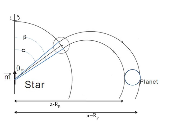
Figure 2: Main parameters in the calculation of $y_{1}$ and $y_{2}$ which defines the geometry of the foot of the flux tube

.

In this model, we make a distinction between the regular (unperturbed) stellar dipole magnetic field (magnetosphere) which co-rotates with the stellar spin and the field lines which define the flux tube (composed of both the stellar field in the planet and the induced flux tube) which appear to be dragged along with the planet and thus move relative to the rest of the stellar magnetosphere. This drag is significant when the electric conductivity of the planet is large compared to that of the outer layers of the star (Piddington & Drake 1968, ).

A large conductivity in the planet’s interior would lead to a large surface current which induces a field and cancels the external (unperturbed stellar dipole) field. With small magnetic diffusivity, the planet’s interior would appear to be shielded from any time dependent external magnetic field. We, therefore, consider only the time-independent component of the stellar magnetic field. In this model, the time-independent component of the stellar magnetic field permeates the planet. The motion of the planet relative to the stellar magnetosphere induces an electric field $\mathcal{E}$, an induced volumic electric current $\mathcal{J}$, and an induced difference of potential U across the planet’s diameter. In Figure 3, we provide a schematic illustration on the field lines and current inside the planet.

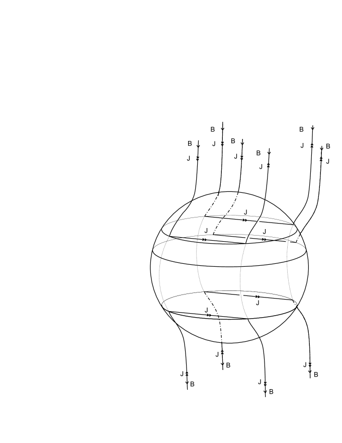
Figure 3: External and induced field around a planet moving relative to the magnetosphere of its host star. The planet is moving out of the plane and toward the lower left side of the illustration. Arrows in this idealized cartoon illustrate the direction of current flow across the potential drop due to the induced emf. The current also lead to an induced field which distorts the field near the planet. Information on the induced emf propagates along the field lines in the direction of the host star.

For the flux tube between the planet and its host star, we adopt the assumption of high electric conductivity along the magnetic field lines and low conductivity across them which was introduced by Goldreich & LyndenBell (1969) for the system Io-Jupiter. In this case, the difference of electric potential (induced by the planet’s relative motion with respect to the magnetic field of its host star) drives an electrical current out of the planet, along the flux tube, across its foot on the atmosphere of the star, and back to the planet along its other half (Figure 1).

In the limit of negligible electrical conductivity in the direction normal to the flux tube, the electric current can only cross the field lines in the planet or in the atmosphere of the host star. The assumption of high electric conductivity along the magnetic field lines also implies 1) that the difference of potential U across the planet’s diameter is transmitted along the flux tube without significant drop in potential and 2) that the plasma enclosed in the flux tube is dragged along by the motion of the magnetic field lines. An electric circuit is therefore created, where the flux tube acts as electric wires, the planet as a unipolar inductor with internal resistance $\mathcal{R}_{p}$, and the foot of the flux tube as the largest resistance.

We see that there are in fact two circuits (see Figure 1). The first one is composed of the foot of the flux tube on the northern hemisphere of the star, its corresponding flux tube, and the northern hemisphere of the planet. The second is equivalent and symmetric to the first one (the plane of symmetry being the plane of the planetary disk). Except when explicitly stated, the calculations (current, resistances, ohmic dissipation, torques, etc.) describe only one circuit (the northern one).

In an electric circuit composed of a generator (with an emf $\int\mathcal{E}{\rm d}l$ and resistance $\mathcal{R}_{g}$ over a length scale $l$) and other resistances along the circuit $\mathcal{R}$ (here primarily the resistance of the foot of the flux tube), the intensity of the current $I$ is determined by $\int\mathcal{E}{\rm d}l-\mathcal{R}_{g}I\approx\int\mathcal{E}{\rm d}l=U=\mathcal{R}I$. With the parameters we have adopted here, we show in Section 5 that the resistance along the flux tube $\mathcal{R}_{\rm tube}$ and the resistance across the planet $\mathcal{R}_{\rm p}$ are small compared to that across the foot of the flux tube on the star $\mathcal{R}_{\ast}$. In this limit, 1) the potential drop across the planet with a radius $R_{p}$ is $U\sim 2\mathcal{E}R_{p}$, 2) the magnitude $U$ is approximately constant along each field lines in the flux tube between the planet and its host star because the resistance of the tube $\mathcal{R}_{\rm tube}$ and the induction are negligible, and 3) the total current is determined by the largest resistance along the circuit, i.e. that at the foot of the flux tube in the stellar atmosphere.

3 Description of the Model: Values of the Parameters, Geometry, Analytical Expressions, and Equation of Evolution of the Planet’s Orbit

3.1 Values of the Parameters for a Fiducial Model

Except when explicitly stated otherwise, we consider a system composed of a super-Earth orbiting closely a young T-Tauri star with a time-independent magnetic dipole. We assume that the magnetosphere co-rotates with the star, and adopt the following numerical values (SI units) for the parameters intervening in the model:

For the star we adopt the following model parameters:
Temperature of the isothermal outer layer: $T_{\ast}=4000$ K,
Radius: $R_{\star}\approx 2R_{\odot}\approx 1.4\times 10^{9}$ m,
Mass: $M_{\star}\simeq M_{\odot}\simeq 2\times 10^{30}$ kg,
Opacity at the photosphere: $\kappa\simeq 3$ ${\rm m}^{2}{\rm kg}^{-1}$ (which is equivalent to taking a surface pressure of about 15 Pa),
Magnetic dipole strength: $m=5.4\times 10^{33}$ ${\rm Am}^{2}$, which corresponds to a magnetic field of 0.2 T (Tesla) $\equiv 2\times 10^{3}$ Gs (Gauss) at the stellar surface (Yang et al. 2008, ), and
Spin period: 8 days (slow-rotator) or 0.8 days (fast-rotator).
We will consider more general stellar models elsewhere.

For a super-Earth, we consider the following case:
Radius: $R_{p}\simeq 2R_{\oplus}\simeq 1.4\times 10^{7}$ m, and
Semi-major axis: $a\simeq 0.04$ AU $\simeq 6\times 10^{9}$ m (which corresponds to a period of 3 days).
In the electrodynamics of super-Earths, the magnitude of $M_{p}$ does not enter explicitly (it does implicitly through the radius) the calculation of the torque, albeit their orbital evolution timescale does depend on it (for example, see Equation (16). The linear speed in a frame co-rotating with the star ($\upsilon_{p/s}=(\omega_{p}-\omega_{\ast})a$) of such a planet orbiting a star rotating slowly is $9\times 10^{4}{\rm ms}^{-1}$ and $4\times 10^{5}{\rm ms}^{-1}$ around a star rotating fast (these are the absolute values).

3.2 Length and Width of the Foot of the Flux Tube in a Spherical Approximation

As defined above, the ”flux tube” refers to the flux tube composed of the field lines of the magnetosphere that pass through and are dragged along by the planet. This flux tube connects the planet and the surface of the star. and its foot penetrates into the star to a depth which will be determined later.

The stellar magnetic field has the geometrical structure of a magnetic dipole field. Thus, the foot of the flux tube at the stellar envelope (the circled area in figure 2) is, at the first order in $\sqrt{{R_{\ast}}/{a}}$, an ellipse which axes have respective lengths

$$y_{1} = \left(\frac{R_{p}}{s}\right)\left(\frac{R_{\ast}}{a}\right)^{3/2},$$ (2)

$$y_{2} = 2R_{p}\left(\frac{R_{\ast}}{a}\right)^{3/2},$$ (3)

$$sin\theta_{F} = \sqrt{\frac{R_{\ast}}{a}}$$ (4)

$$cos\theta_{F} = \sqrt{1-\frac{R_{\ast}}{a}}\equiv s,$$ (5)

where $\theta_{F}$ is the angle between the stellar spin axis and the location of the foot of the flux tube. When the current J crosses the foot of the flux tube in the stellar envelope, it covers a length $y_{1}$. In the rest of the paper, we take $cos\theta_{F}$ is roughly equal to 1. We represent it with the symbol s in analytical equations and take it to be equal to 1 in numerical applications.

In Figure 4, we zoom in on the foot of the flux tube at the stellar atmosphere. In order to derive $y_{1}$ and $y_{2}$ (at the first order in ${R_{\ast}}/{a}$), we first solve $\mathcal{B}\wedge dl=0$ and obtain $sin\alpha=\sqrt{\frac{R_{\ast}}{a+R_{p}}}$ and $sin\beta=\sqrt{\frac{R_{\ast}}{a-R_{p}}}$ with $\alpha$ and $\beta$ defined in Figure 2. We then write $y_{1}=R_{\ast}(\alpha-\beta)$ and $y_{2}=\frac{2R_{p}}{2\pi a}2\pi R_{\ast}sin\theta_{F}$.

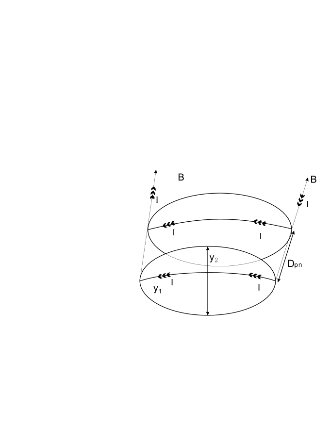
Figure 4: Penetration of the flux tube in the stellar atmosphere. Potential difference across the planet would be maintained at its foot print on the surface of its host star if there is sufficient time for the Alfven waves to transit this information. Arrows indicate the flow direction of the electrical current. The values of $y_{1}$ and $y_{2}$ are given by Equations (2). The top circle represents the stellar surface and the penetration depth $D_{pn}=R_{\ast}-r_{pn}$ is evaluated in Section 5.3.

For a super-Earth (using the model parameters listed above), we find $y_{1}=1.6\times 10^{6}$ m and $y_{2}=3.2\times 10^{6}$ m. For a hot-Jupiter, we would typically need to multiply these values by a factor $10$. The height of the foot of the flux tube is derived below in Section 5.3.3. The numerical applications are for $s=1$. For semi-major axes comparable to the stellar radius, the multiplicative factor $(1-{R_{\ast}}/{a})^{-1/2}$ in $y_{1}$ would significantly affect the length of the foot of the flux tube.

3.3 Induced Difference of Potential

The planet is a conductor moving in the stellar magnetosphere with relative linear speed $\upsilon_{p/s}$. Modeling the stellar magnetic field as the one created by a magnetic dipole (of magnetic moment m), the magnitude of the induced electric field in the planet $\mathcal{E}_{p}$ is

$$\mathcal{E}_{p}=\upsilon_{p/s}\mathcal{B}_{\ast}(a)=(\omega_{p}-\omega_{\ast})a\frac{\mu_{0}m}{4\pi a^{3}}$$ (6)

with $\mathcal{B}_{\ast}(a)$ represents the stellar magnetic field at the location of the planet. Numerical applications for a super Earth give $\mathcal{E}_{p}=240$ V ${\rm m}^{-1}$ (slow-rotator), $1000$ V${\rm m}^{-1}$ (fast rotator) (a slow or fast rotator depends on the spin frequency of the star, as described in section 3.1).

The magnitude of the difference of potential U (or emf) generated across the planet is thus

$$U=2R_{p}\mathcal{E}_{p}=2R_{p}(\omega_{p}-\omega_{\ast})a\frac{\mu_{0}m}{4\pi a^{3}}.$$ (7)

For the super-Earth models under consideration, $U=6.7\times 10^{9}V$ (slow rotator) and $2.8\times 10^{10}V$ (fast-rotator). This difference of potential is transmitted across the flux tube (with the assumption of infinite conductivity along the flux tube that passes through the planet) and generates a uniform electric field $\mathcal{E}_{\ast}$ in the stellar envelope (see Figure 1) at the foot of the flux tube

$$\mathcal{E}_{\ast}=\frac{U}{y_{1}}=2\frac{\mu_{0}m}{4\pi a^{3}}(\omega_{p}-\omega_{\ast})a\left(\frac{a}{R_{s}}\right)^{3/2}s.$$ (8)

The value of $\mathcal{E}_{\ast}$ does not depend on the radius of the planet, and for our values of the parameters for a young T Tauri star, $\mathcal{E}_{\ast}=4.2\times 10^{3}$V$m^{-1}$ (slow rotator), $1.8\times 10^{4}$V$m^{-1}$ (fast rotator).

3.4 Analytical Expressions: Intensity in the Circuit, Ohmic Dissipation, and Torque in the Planet and Star

The induced current I is given by

$$I=\int_{z}\int_{y}\mathcal{J}dydz=\mathcal{E}_{\ast}y_{2}\int_{z}\sigma_{\ast}(z)dz=U\frac{y_{2}}{y_{1}}\int_{z}\sigma_{\ast}(z)dz=4R_{p}(\omega_{p}-\omega_{\ast})a\frac{\mu_{0}m}{4\pi a^{3}}s\int_{z}\sigma_{\ast}(z)dz.$$ (9)

In the previous equation, $\mathcal{J}$ is the volumic electric current in the stellar atmosphere at the foot of the flux tube (induced by U), y varies from 0 to $y_{2}$ (the width of the foot of the flux tube), and z varies from $r_{pn}$ (the radius to which the flux tube can penetrate into the stellar atmosphere) to $R_{\ast}$ and $\frac{y_{2}}{y_{1}}=2s$ (see Figure 4). In this circuit, the total resistance is the sum of that across the planet, the foot print of the flux tube on the stellar surface, and along the flux tube. Here we consider only the largest contribution and neglect that across the planet. In Section 5.3, we determine the magnitude of $r_{pn}$ and evaluate

$$\Sigma=\int_{r_{pn}}^{R_{\ast}}\sigma_{p}(z)dz$$ (10)

such that $I=2U\Sigma s$. In the above equation, $\sigma_{p}(z)$ is the local Pedersen conductivity (see Equation 47). The total resistance of the stellar atmosphere at the foot of the flux tube is

$$\mathcal{R}_{\ast}=\frac{U}{I}=\frac{y_{1}}{y_{2}}\frac{1}{\Sigma}=\frac{1}{2\Sigma s}.$$ (11)

The total ohmic power dissipation in the stellar atmosphere at the foot of both flux tubes (one for each hemisphere, thus the multiplicative factor 2) $\mathcal{P}_{\ast}$ and in the planet $\mathcal{P}_{p}$ are

$$\mathcal{P}_{\ast} = 2\mathcal{R}_{\ast}I^{2}=2UI=4U^{2}\Sigma s=16R_{p}^{2}(\omega_{p}-\omega_{\ast})^{2}a^{2}\left(\frac{\mu_{0}m}{4\pi a^{3}}\right)^{2}\Sigma s$$ (12)

$$\mathcal{P}_{p} = 2\mathcal{R}_{p}I^{2}=2\mathcal{R}_{p}\left(2U\Sigma s\right)^{2}=\mathcal{P}_{\ast}\frac{\mathcal{R}_{p}}{\mathcal{R}_{\ast}}$$ (13)

where $\mathcal{R}_{\ast}$ is the resistance of the foot of the flux tube (on one hemisphere), and $\mathcal{R}_{p}$ is the resistance of one hemisphere of the planet. Since the resistance in the planet is considerably smaller than that in the star, most of the power is dissipated in near the foot of the flux tube on the surface of the star. Note that the magnitude of both $\mathcal{P}_{\ast}$ and $\mathcal{P}_{p}$ is determined by $I$ and $\mathcal{R}_{\ast}$.

The total torque (for both circuits, one circuit for each hemisphere) due to the Lorentz force (the axis is the stellar spin axis) on the star (equal in absolute value to that on the planet) is

$$\mathcal{T}_{\ast} = 2\int_{x}\int_{y}\int_{z}r\wedge(\mathcal{J}\wedge\mathcal{B})dxdydz=2(R_{\ast}sin\theta_{F})(y_{1}I)(\frac{2\mu_{0}mcos\theta_{F}}{4\pi R_{\ast}^{3}})=4R_{p}a\frac{\mu_{0}m}{4\pi a^{3}}I\textbf{e}_{z},$$ (14)

$$\mathcal{T}_{\ast} = 16R_{p}^{2}a^{2}(\omega_{p}-\omega_{\ast})\left(\frac{\mu_{0}m}{4\pi a^{3}}\right)^{2}\Sigma s\textbf{e}_{z}$$ (15)

where $s=cos\theta_{F}$ as defined in (2) and I is the integral of the volumic current across a cross section (we take an averaged view of the volumic current rather than determining its complex geometry inside the planet). We have calculated here the total ohmic dissipation and torque (i.e. for both hemispheres).

3.5 Equation of Evolution of the Stellar Spin and Planet’s Orbital Angular Velocity and Semimajor Axis

The torque on the planet $\mathcal{T}_{p}$ is equal and opposite that on the star $\mathcal{T}_{\ast}$. Consequently, the semimajor axis of a super-Earth on a circular orbit evolves at a rate

$${\dot{a}}=\frac{2a}{H_{p}}\mathcal{T}_{p}$$ (16)

where the total angular momentum of the planet’s orbit is $H_{p}=M_{p}a^{2}\omega_{p}$. Since the total angular momentum of the system is conserved, the changing rate of the stellar spin is

$${\dot{\omega}_{\ast}}=\frac{\mathcal{T}_{\ast}}{c_{\ast}M_{\ast}R_{\ast}^{2}}$$ (17)

where $c_{\ast}\simeq 2/5$ is the inertial constant of the star. According to the above expression, the planet would undergo orbital decay and its host star would spin up if it is inside corotation (or equivalently if $\omega_{p}>\omega_{\ast}$). Similarly, the planet’s orbit would expand and its host star would spin down if it is outside corotation.

The planet’s orbital frequency $\omega_{p}$ is related to the semi-major axis $\omega_{p}=\frac{\sqrt{GM_{\ast}}}{a^{3/2}}$. Using the expressions calculated for the torques and Equations (16) and (17), we find

$$\stackrel{{\scriptstyle\centerdot}}{{\omega}}_{\ast}=\frac{M_{p}(GM_{\ast})^{2/3}}{3C_{\ast}M_{\ast}R_{\ast}^{2}}\frac{\stackrel{{\scriptstyle\centerdot}}{{\omega_{p}}}}{\omega_{p}^{4/3}}\approx 3\times 10^{-10}\frac{\stackrel{{\scriptstyle\centerdot}}{{\omega}}_{p}}{\left(\omega_{p}\stackrel{{\scriptstyle\sim}}{{s}}\right)^{4/3}}$$ (18)

where the numerical application was for a planet with 10 Earth Masses ($M_{p}=6\times 10^{25}$kg) and $\rm\stackrel{{\scriptstyle\sim}}{{s}}$ represent second. Therefore, we can estimate the variation of $\omega_{\ast}$ during the evolution of the planet’s migration

$$\mid\bigtriangleup\omega_{\ast}\mid=-\frac{M_{p}(GM_{\ast})^{2/3}}{C_{\ast}M_{\ast}R_{\ast}^{2}}\mid\bigtriangleup\left(\frac{1}{\omega_{p}^{1/3}}\right)\mid$$ (19)

which is negligibly small.

We can thus consider that the star’s angular velocity is roughly unaffected by this transfer of angular momentum. Using Equation (16), $a^{3}=\frac{GM_{\ast}}{\omega^{2}_{p}}$, $\frac{\stackrel{{\scriptstyle\centerdot}}{{a}}}{a}=\frac{-2}{3}\frac{\stackrel{{\scriptstyle\centerdot}}{{\omega_{p}}}}{\omega_{p}}$, and the expression for the torque on the planet (equal to $-\mathcal{T}_{\ast}$ with $\mathcal{T}_{\ast}$ given in Equation (15)) we find

$$\frac{\stackrel{{\scriptstyle\centerdot}}{{\omega_{p}}}}{\omega_{p}^{4}(\omega_{p}-\omega_{\ast})}=48\frac{R_{p}^{2}}{M_{p}}\left(\frac{\mu_{0}m}{4\pi}\right)^{2}\frac{\Sigma s}{(GM_{\ast})^{2}}=\alpha$$ (20)

where $\omega_{\ast}$ is constant and $\alpha=48\frac{R_{p}^{2}}{M_{p}}\left(\frac{\mu_{0}m}{4\pi}\right)^{2}\frac{\Sigma s}{(GM_{\ast})^{2}}$ (of unit $s^{3}$), and s in the numerator of the expression for $\alpha$ is defined as in 2. The previous equation becomes

$$-\frac{1}{\omega_{\ast}}\frac{\stackrel{{\scriptstyle\centerdot}}{{\omega_{p}}}}{\omega_{p}^{4}}-\frac{1}{\omega_{\ast}^{2}}\frac{\stackrel{{\scriptstyle\centerdot}}{{\omega_{p}}}}{\omega_{p}^{3}}-\frac{1}{\omega_{\ast}^{3}}\frac{\stackrel{{\scriptstyle\centerdot}}{{\omega_{p}}}}{\omega_{p}^{2}}-\frac{1}{\omega_{\ast}^{4}}\frac{\stackrel{{\scriptstyle\centerdot}}{{\omega_{p}}}}{\omega_{p}}+\frac{1}{\omega_{\ast}^{4}}\frac{\stackrel{{\scriptstyle\centerdot}}{{\omega_{p}}}}{(\omega_{p}-\omega_{\ast})}=\alpha.$$ (21)

After integration, we find

$$\frac{\Omega^{3}(t)}{3}+\frac{\Omega^{2}(t)}{2}+\Omega(t)+ln\left(\mid 1-\Omega(t)\mid\right)=\frac{\Omega^{3}_{i}}{3}+\frac{\Omega^{2}_{i}}{2}+\Omega_{i}+ln\left(\mid 1-\Omega_{i}\mid\right)+\alpha\omega_{\ast}^{4}(t-t_{0})$$ (22)

where we define $\Omega(t)\equiv{\omega_{\ast}}/{\omega_{p}(t)}$ and $\Omega_{i}\equiv\Omega(t=t_{0})$.

Near co-rotation (i.e. $\Omega\simeq 1$), the ln function is dominant and we find

$$ln\left(\mid 1-\Omega(t)\mid\right)=ln\left(\mid 1-\Omega_{i}\mid\right)+\alpha\omega_{\ast}^{4}(t-t_{0}).$$ (23)

If $\omega_{p}$ is greater than $\omega_{\ast}$, then

$$\frac{\omega_{p}(t)}{\omega_{\ast}}=\frac{1}{\Omega(t)}=\left[1-\left(1-\frac{\omega_{\ast}}{\omega_{p}(t_{0})}\right)exp\left(\alpha\omega_{\ast}^{4}(t-t_{0})\right)\right]^{-1}.$$ (24)

Similarly, if $\omega_{p}$ is less than $\omega_{\ast}$, then

$$\frac{\omega_{p}(t)}{\omega_{\ast}}=\frac{1}{\Omega(t)}=\left[1+\left(\frac{\omega_{\ast}}{\omega_{p}(t_{0})}-1\right)exp\left(\alpha\omega_{\ast}^{4}(t-t_{0})\right)\right]^{-1}.$$ (25)

and the planet-star system approaches co-rotation with a timescale

$$\tau=\frac{1}{\alpha\omega_{\ast}^{4}}=\frac{M_{p}(GM_{\ast})^{2}}{48\omega_{\ast}^{4}R_{p}^{2}\Sigma s}\left(\frac{\mu_{0}m}{4\pi}\right)^{-2}.$$ (26)

In the general case, $\omega_{p}(t)$ follows Equation (22), or written differently:

$$\omega_{p}^{3}(t)\left[f(t)-ln\mid 1-\frac{\omega_{\ast}}{\omega_{p}(t)}\mid\right]-\omega_{\ast}\omega_{p}^{2}(t)-\frac{\omega_{\ast}^{2}}{2}\omega_{p}(t)=\frac{\omega_{\ast}^{3}}{3}$$ (27)

where $f(t)=A+B(t-t_{0})$ with $A={\Omega^{3}_{i}}/{3}+{\Omega^{2}_{i}}/{2}+\Omega_{i}+ln\left(\mid 1-\Omega_{i}\mid\right)$ and $B={\alpha\omega_{\ast}^{4}}.$

In order to get an equation of evolution of the semi-major axis, one can replace in Equation (23, near co-rotation) or (22, in the general case) $\Omega_{p}(t)$ by $\left({a(t)}/{a_{c}}\right)^{3/2}$ and $\Omega_{i}$ by $\left({a(t_{0})}/{a_{c}}\right)^{3/2}$ with $a_{c}$ the co-rotation radius. Near co-rotation, we find

$$a(t)=a_{c}\left[1-\left[1-\left(a(t_{0})\over a_{c}\right)^{3/2}\right]{\rm exp}\left({t-t_{0}\over\tau}\right)\right]^{2/3}$$ (28)

for the case where a is smaller than $a_{c}$.

4 Condition for the validity of the Model: $t_{A}\leq t_{max}$

In order to apply the model described above, one needs to verify that the time $t_{A}$ required for the Alfven waves to travel along the flux tube (to a depth $D_{pn}$ inside the star to be determined), and back to the planet is smaller than the time $t_{max}$ it takes the flux tube to slip ahead of the planet by more than its diameter. This condition ensures that a perturbation along a field line of the flux tube has the time to travel back and forth while the field line is still part of the flux tube that passes through the planet. Figures 5 and 6 illustrate this condition. Figure 7 shows the field lines near the planet in the case where the condition is not met.

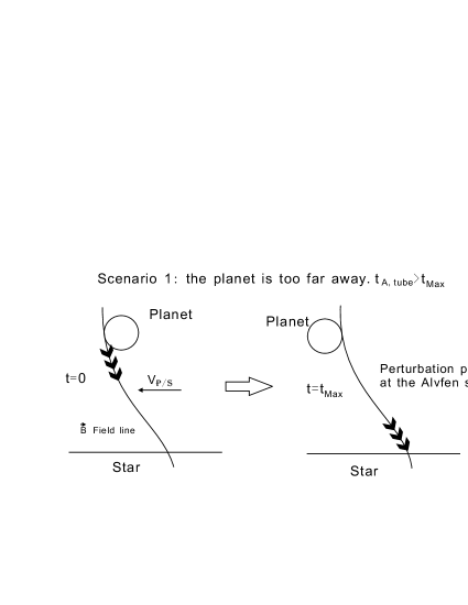
Figure 5: Propagation of the Alfven wave between a relatively distant planet and its host star. The planet’s motion relative to the stellar field induces a potential drop across the flux tube in the proximity of the planet. This information propagates along the flux tube toward the host star with an Alfven speed. Due to finite diffusion and the relative motion between the planet and the stellar magnetosphere, the net field lines also slip through the planet. In this illustration the timescale required for the Alfven wave to reach the host star is long compared with that required for the slippage of the field. The circuit is not established in this case.

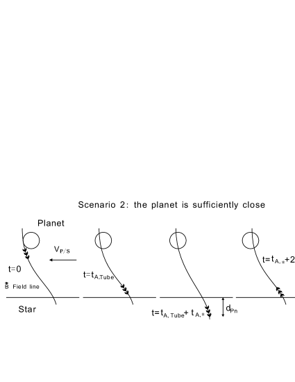
Figure 6: Necessary condition for a complete unipolar inductor circuit. Similar to the illustration in Figure 5, the potential drop across the planet propagates along the flux tube toward the planet with an Alfven speed. In this illustration, the planet is sufficiently close to its host star that the potential drop can be established on the surface of the host star before the fields slip through the planet. This potential drop induces a current which is determined by the resistivity on the stellar surface. In this case, it is possible to complete the circuit induced by the motion of the planet.

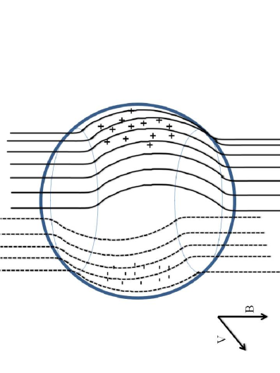
Figure 7: Magnetic field lines in the case where the circuit is not closed. The planetary motion relative to the stellar magnetic field induces charge separation. Without any connection (at infinity) between the separated charges, there is no current in the frame of the moving planet. In a infinitely conducting planet, the separated charges are concentrated near its surface. The magnitude of the induced field $\mathcal{E}_{p}$ is determined by Equation (6). In the stationary frame (centered on the host star), the separated surface charges carried by the planets generate two opposite currents as well as a finite $\nabla\wedge\mathcal{E}_{p}$ in the moving planet. Interior to the infinitely conducting moving planet, the induced field exactly cancels the unperturbed field as if there is no diffusion of the stellar magnetic field into the planet. In the external region close to the moving planet, the induced field strongly perturbs the stellar magnetic field. The net field distortion is symmetric around an infinitely conducting moving planet (analogous to an invisic flow around a spherical object) such that there is no net torque acting between the planet and the stellar field. This symmetry would be broken and the drag on the planet would be finite if its conductivity is sufficiently low to permit significant slippage of the stellar magnetic field or if a complete circuit connecting two sides of the planet can be established on the surface of its host star.

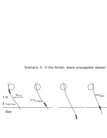
Figure 8: Penetration depth of the unipolar induction circuit. The propagation of the induced disturbances from the planet to the stellar surface is $t_{A,tube}$. Below the stellar surface, gas density increases exponentially and the Alfven speed decreases accordingly. The penetration depth of the planet’s induced field is determined by the requirement that the timescale for the Alfven waves to complete the circuit equals to the field slippage timescale across the planet. The net resistivity at the stellar surface is determined by the gas across the flux tube in the form of parallel resistors.

In order to calculate $t_{A}$, we need to estimate the Alfven speeds along the flux tube between the planet and the star and in the stellar ionosphere (at the foot of the flux tube). Similarly, the calculation of $t_{max}$ requires the value of the conductivities (or resistance) of the different components of the circuit. Indeed, the ratio of $\mathcal{R}_{p}$ (resistance of the planet) and $\mathcal{R}_{\ast}$ (resistance of the foot of the flux tube in the stellar atmosphere) determines the amount of relative slippage between the flux tube and the planet (Dermott 1970, ).

In the limit where $\mathcal{R}_{p}$ is comparable to or larger than $\mathcal{R}_{\ast}$ (as in the night side of synchronously spinning hot Jupiter, see Paper I), the flux tube would tend to slip through the planet. In this case, the flux tube would slip ahead of the planet by a distance $\sim 2R_{p}$ in a relatively short time $t_{A}$, and it might not be possible to maintain a closed circuit.

In the most unfavorable case ($\mathcal{R}_{p}/\mathcal{R}_{\ast}=\infty$, i.e. the flux tube passes through the planet completely undisturbed), $t_{A}={2R_{p}}/{\upsilon_{p/s}}$ (where $\upsilon_{p/s}$ represents the speed of the planet in the frame rotating with the stellar magnetosphere). In the opposite extreme limit, $\mathcal{R}_{p}/\mathcal{R}_{\ast}=0$ and $t_{A}=\infty$ such that the flux tube is completely anchored in the planet. Differential motion steadily stretch the field lines until they reconnect. A more realistic situation falls somewhere between these two extreme limits, and the smaller $\mathcal{R}_{p}/\mathcal{R}_{\ast}$, the easier it is to satisfy the condition of validity.

4.1 Qualitative Estimate of the Relative Slippage

A first qualitative criterion is given by the following argument. We want to determine whether the magnetic flux tube slips on the planet or on the star. In the absence of any companions, the magnetic field in the magnetosphere of a star rotates with the star. A close-in planet would tend to drag the stellar magnetic field lines that pass through it along with its motion.

Let us define $\omega_{p}$, $\omega_{\ast}$, and $\omega_{B}$ to be the angular velocity of the planet, star, and magnetic field in an absolute frame. We then consider the relative motion between the planet and the field lines, and between the field lines and the star. We write $\Omega_{p}=\omega_{p}-\omega_{B}$ and $\Omega_{\ast}=\omega_{B}-\omega_{\ast}$ and our goal is to estimate the magnitude of $\Omega_{p}/\Omega_{\ast}$. In these notations, the planet’s speed relative to the magnetic field is then $\upsilon_{p}=\Omega_{p}\ a$ ($a$ is the semi-major axis), and the speed of the field lines (that pass through the planet) relative to the star is $\upsilon_{\ast}=\Omega_{\ast}R_{\ast}$ ($R_{\ast}$ being the stellar radius).

Considering the DC component of the field, we can write the complete MHD induction equation (see Equation (1)) for the star and the planet.

$$\frac{\partial\stackrel{{\scriptstyle\rightarrow}}{{\mathcal{B}}}_{p}}{\partial t} = \nabla\wedge(\stackrel{{\scriptstyle\rightarrow}}{{\upsilon}}_{p}\wedge\stackrel{{\scriptstyle\rightarrow}}{{\mathcal{B}}}_{p})+\nabla\wedge(\eta_{p}\nabla\wedge\stackrel{{\scriptstyle\rightarrow}}{{\mathcal{B}}}_{p})$$

$$\frac{\partial\stackrel{{\scriptstyle\rightarrow}}{{\mathcal{B}}}_{\ast}}{\partial t} = \nabla\wedge(\stackrel{{\scriptstyle\rightarrow}}{{\upsilon}}_{\ast}\wedge\stackrel{{\scriptstyle\rightarrow}}{{\mathcal{B}}}_{\ast})+\nabla\wedge(\eta_{\ast}\nabla\wedge\stackrel{{\scriptstyle\rightarrow}}{{\mathcal{B}}}_{\ast}).$$ (29)

In a steady state, the first and second equations imply $\upsilon_{p}\approx{\eta_{p}}/{R_{p}}$ and $\upsilon_{\ast}\approx{\eta_{\ast}}/{R_{\ast}}$, respectively. Therefore, we obtain

$$\frac{\Omega_{p}}{\Omega_{\ast}}\approx\frac{\sigma_{\ast}}{\sigma_{p}}\ \frac{R_{\ast}^{2}}{R_{p}a}.$$ (30)

In the context of Io-Jupiter interaction ${R_{\ast}^{2}}/{R_{p}a}\approx 7$. Since the electrical conductivity on Io is estimated to be much larger than that on Jupiter, the flux tube which passes through Io moves with Io and drags its foot on the surface of Jupiter (Goldreich & Lynden-Bell 1969, ). For a Jupiter-mass planet orbiting a young T-Tauri star (with radius twice that of the sun) at 0.04 AU (3 day-period), ${R_{\ast}^{2}}/{R_{p}a}\approx 4$, and the anchorage of the flux tube which passes through the hot Jupiters is thus determined by the ratio of the diffusivity through the planet to that through its host star. For a super-Earth with radius twice that of the earth at 0.04 AU, ${R_{\ast}^{2}}/{R_{p}a}\approx 20$.

4.2 Analytical Expression of the Time Constraint, $t_{max}$

The magnitude of $t_{max}$ is the time it takes for the field lines in the flux tube to slip pass through the planet by a distance equal to the planetary diameter. We consider a planet with an electrical conductivity $\sigma_{p}$ moving relative to a magnetic field at speed $\upsilon_{p/s}=(\omega_{p}-\omega_{\ast})a$. If the planet does not drag the field at all (for example if $\sigma_{p}=0$), the field lines would move relative to the planet with a linear speed $\upsilon_{p/s}$. Thus, the minimum value for $t_{max}$ is $t_{max}={2R_{p}}/{\upsilon_{p/s}}$. On the other hand, if the field lines are perfectly anchored in the planet (for example when $\sigma_{p}=\infty$) then $t_{max}=\infty$. The induced field lines would wrap around the host stars with the planet’s synodic orbit (i.e. its motion relative to the stellar spin).

Based on extrapolation from analogous considerations (Aly 1985, Aly & Kuijpers, van Ballegooijen 1994), we hypothesize that magnetic reconnection may occur when the azimuthal component of the induced (and “dragged”) magnetic field well outside the planet becomes comparable to the unperturbed stellar dipole field. We assume the time growth timescale for the azimuthal component of the field to the period $t_{syn}=2\pi/(\omega_{p}-\omega_{\ast})$ of the planet’s synodic period. If it occurs, reconnection would lead to short-circuit and a burst of intense ohmic dissipation in the planet. We discuss the possibility of magnetic reconnection again in section (6.4). In the limit of infinite $t_{max}$, the relative motion between the planet and the stellar field would restore the electric field and re-establish the circuit on the timescale of $t_{A}$ with a reduced effective conductivity (or equivalently an enhanced resistivity and magnetic diffusivity). We shall consider elsewhere the possibility of such an episodic electrodynamic process.

In general, the conductivity $\sigma_{p}$ would fall between $0$ and $\infty$ and the field is dragged without being completely anchored on the planet. The induced field lines are distorted and partially wrapped around the host star. In the limit that $t_{A}<t_{max}<t_{syn}$, it is possible to complete a steady circuit of unipolar induction without reconnection.

The same argument also holds for the star with electrical conductivity $\sigma_{\ast}$ dragging its own field lines so that the intensity of the slippage between the field lines and the planet depends on both the conductivity of the planet and star. Modeling the interaction between Io and Jupiter, Goldreich & Lynden-Bell (1969) took into account $\sigma_{Io}$ and $\sigma_{Jupiter}$. Dermott (1970) included the contribution of the flux tube’s conductivity in the expression of the slippage of the field relative to both Io and Jupiter.

In the present context, the linear speed of the slippage between the flux tube and the planet is

$$\upsilon_{slip}=\frac{\upsilon_{p/s}}{1+(\mathcal{R}_{\ast}+\mathcal{R}_{tube})/(\mathcal{R}_{tube}+\mathcal{R}_{p})}.$$ (31)

(In the above expression, we use $\mathcal{R}_{p}$ instead of $2\mathcal{R}_{p}$ as in Dermott).

In a complete circuit, the maximum time available for the Alfven waves to propagate from the planet to the star and return to the planet is

$$t_{max}=\frac{2R_{p}}{\upsilon_{slip}}=2R_{p}\frac{(1+w)}{(\omega_{p}-\omega_{\ast})a}$$ (32)

where $w={(\mathcal{R}_{\ast}+\mathcal{R}_{tube})}/{(\mathcal{R}_{p}+\mathcal{R}_{tube})}$. It is common to neglect $\mathcal{R}_{tube}$.

5 Resistance and Alfven speed along the circuit

We derived the analytical expressions of the total intensity (Section 3.4) and the time available for the Alfven waves to travel back and forth between the planet and the foot of the flux tube (Section 4.2). In order to determine their numerical values, we calculate in this section 1) the planet’s integrated resistance $\mathcal{R}_{p}$, 2) the resistance $\mathcal{R}_{tube}$ and Alfven speed $\upsilon_{A,tube}$ along the flux tube, 3) and the resistance across the foot of the flux tube just below the star’s surface $\mathcal{R}_{\ast}$ (perpendicular to the magnetic field and parallel to the electric potential gradient) and the Alfven speed along the foot of the flux tube $\upsilon_{A,tube}$. Figures 5 and 6 provide a summary of the condition of validity.

5.1 Resistance in the Planet $\mathcal{R}_{p}$

The electrical conductivity profile of a super-Earth is unclear. We thus first discuss the (better characterized) conductivity profile of present day Earth. Lorrain et al. (2006) estimated the electric conductivity of the present-day Earth mantle to range between $10^{-2}\ {\rm ohm}^{-1}\ {\rm m}^{-1}$ and $10^{3}\ {\rm ohm}^{-1}\ {\rm m}^{-1}$ and $10^{5}\ {\rm ohm}^{-1}\ {\rm m}^{-1}$ for the inner core (also see Stevenson, 2003). Merrill et al. (1996, pp. 273-277) similarly argues for an electrical conductivity of about 5-8 $\times 10^{5}\ {\rm ohm}^{-1}\ {\rm m}^{-1}$ for the core of the Earth, and between 3 and 100 ${\rm ohm}^{-1}\ {\rm m}^{-1}$ for the lower mantle. For the upper mantle (and crust), Obiekezie & Okeke (2010) calculate an electrical conductivity increasing from the surface (about $3\times 10^{-2}\ {\rm ohm}^{-1}\ {\rm m}^{-1}$) to $10^{-1}\ {\rm ohm}^{-1}\ {\rm m}^{-1}$ at around 500km. The electrical conductivity of the Earth is therefore minimal and between $3\times 10^{-2}\$ and $10^{-1}{\rm ohm}^{-1}\ {\rm m}^{-1}$) for a few hundred kilometers and then increase with depth.

In the present application, we are primarily interested in the interaction between super-Earths and their host stars when they are relatively young (up to a few $10^{7}$ yr). During this stage, the stellar magnetic field is intense and the close-in super-Earths may be intensely heated by giant impacts, tidal and ohmic dissipation. Super-Earths with a molten crust are likely to have higher conductivities than the present-date terrestrial planets (for example, Rikitake (1966) expressed the conductivity of rocks and metals on the Earth as a sum of $exp(-E_{i}/kT)$, and Umemoto et al. (2006) estimated a conductivity at the core of a super-Earth and hot-Jupiter to be around $10^{6}\ {\rm ohm}^{-1}\ {\rm m}^{-1}$). The stellar radiation alone would raise the super-Earth surface temperature to about 1500K. Ohmic dissipation inside the planet may provide an additional source of thermal energy (see Section 6.3). In a thermal equilibrium, the planet’s surface temperature may sometimes exceed 2000K, at which silicate melts and raise the electric conductivity to around 10 ${\rm ohm}^{-1}\ {\rm m}^{-1}$ (for 1400K, Waff & Weill, 1975).

It is therefore reasonable to assume that the electrical conductivity of a super-Earth is most likely higher but at least that of the Earth. The electrical conductivity in a super earth would thus be several order of magnitude higher than $1\ {\rm ohm}^{-1}\ {\rm m}^{-1}$ in the core and lower mantle and arguably also in the upper mantle. Besides, a conductivity of 0.1-$1\ {\rm ohm}^{-1}\ {\rm m}^{-1}$ (i.e. 10 times lower than the value we use) in an area spanning 10 % of the planet (roughly the thickness of the upper mantle) would at most double total the resistance.

In addition, for a super-Earth, the characteristic speed (for example the planet linear speed in a frame co-rotating with the star) is much faster that for the field to diffuse across it, i.e. $\upsilon\gg\frac{\eta}{L}=\frac{1}{\mu_{0}\sigma L}$ where $L$ is the characteristic length. Therefore, we can neglect the diffusion (second term on the right hand side of the MHD equation (Equation (1)) compared to the induction (first term).

The integrated resistance in the geometry of the planet is

$$\mathcal{R}_{p}=\frac{1}{S}\frac{L}{\sigma}=\frac{1}{R_{p}\sigma_{p}}$$ (33)

where $S$ is the cross section. Depending of the geometry of the current inside the planet, the formula could have multiplicative factors, usually of order unity.

With these approximations, we find

$$\mathcal{R}_{p}=\frac{1}{R_{p}\sigma}\ll 7\times 10^{-8}{\rm Ohm}$$ (34)

The value we use in our fiducial calculation is $\mathcal{R}_{p}=7\times 10^{-8}{\rm Ohm}$. If our assumption that the conductivity in a super-Earth is higher than that in the present-day Earth is inappropriate, this resistance could be higher. But it may also be much lower if the super-Earth has a substantial atmosphere which is extensively photo-ionized or a fully molten core where the alkali metals are partially ionized.

5.2 Resistance and Alfven Speed Along the Flux Tube

Electrodynamics along the flux tube determines the propagation of the induced electric field between the planet and its host star. The total resistance along the flux tube determines changes in the electric potential at the foot of the flux tube. The Alfven speed determines the propagation speed of the disturbance.

5.2.1 Total Resistance Along the Flux Tube $\mathcal{R}_{tube}$

The resistance of the flux tube is also difficult to estimate accurately. Goldreich & Lynden-Bell (1969) simply assumed the electric conductivity to be infinite along the magnetic field lines and did not include $\mathcal{R}_{tube}$ in their equations. Dermott included $\mathcal{R}_{tube}$ in the equations but, during numerical applications, assumed it to be negligible in front of the resistance of the satellite Io. In all previous investigations, conductivity across the field lines in the tenuous region between the planet and the star is assumed to be negligible.

We provide here an estimate of the order of magnitude of the resistance of the flux tube. If we assume the plasma between the star and the planet to be fully ionized, the electric conductivity along (parallel) to the magnetic field line would

$$\sigma_{0}=\frac{n_{e}e^{2}}{m_{e}\nu_{e}}$$ (35)

where $n_{e}$ is the volumic number of free electrons, $e$ and $m_{e}$ are the charge and mass of the electron, and $\nu_{e}$ the collisional frequency of the electrons with electrons and ions/protons (we assume these two collisional frequency to be the same).

We take $\nu_{e}=\frac{n_{e}e^{4}}{16\pi\epsilon_{0}^{2}m_{e}^{2}<\upsilon_{e}>^{3}}$ with the electron thermal speed $<\upsilon_{e}>=\sqrt{\frac{2k_{B}T}{m_{e}}}$. We thus get $\nu_{e}=n_{e}1.2\times 10^{-6}T^{-3/2}$ and $\sigma_{0}=\frac{e^{2}T^{3/2}}{1.2\times 10^{-6}m_{e}}$. In our model, we consider a star with a surface temperature $T_{\ast}=4000$K, and a planet with the equilibrium temperature $T_{p}\sim 1,500$K for the planet with an $a=$ 0.04 AU. For an average temperature of 2000K between the star and the planet, we find $\sigma_{0}\simeq 2000\ {\rm Ohm}^{-1}\ {\rm m}^{-1}$ so that

$$\mathcal{R}_{tube}=\frac{L}{\sigma_{0}S}=\frac{a}{(\pi R_{p})(R_{p}f_{tube})\sigma_{0}}=\frac{4.6\times 10^{-9}}{f_{tube}}{\rm Ohm}$$ (36)

where $f_{tube}$ is between $0$ and $1$ such that $R_{p}f_{tube}$ is equal to the thickness of the volumic current that flows along the field lines. This resistance is usually negligible compared to the other resistances involved in the model (especially that of the star), except if the volumic currents are confined in an extremely thin layer at the surface of the flux tube. Therefore, we neglect the potential difference, along each field line in the flux tube between the surfaces of the planet and star.

5.2.2 Travel Time Along the Flux Tube Between the Planet and (the Top of) the Stellar Surface

We assume that the plasma between the star and the planet is fully ionized and estimate $\upsilon_{A,tube}$ under various different situations.

1) We first consider the epoch shortly after the super-Earth has migrated to the stellar proximity through planet-disk tidal interaction. In opaque inner regions of their natal disks, super-Earths’ type I migration generally stalls at a radius $r$ where the $\Sigma_{d}$ has a positive radial gradient with a scale height $\Delta r=\Sigma_{d}/(\partial\Sigma_{d}/\partial r)$ which is a fraction ($\sim 0.1-0.2$) of $r$ (Masset et al 2006, ). Special locations include narrow transition regions between active inner region and dead zone as well as outer edge of magnetospheric cavity (Kretke et al. 2009, ).

We consider a super-Earth is embedded in a disk with an effective thickness $H_{d}\simeq c_{s}/\omega_{p}\sim 0.01-0.1r$ and a steady state mass transfer rate ${\dot{M}}_{d}=2\pi\Sigma_{d}U_{a}r$ throughout the disk where $\Sigma_{d}$ and $c_{s}$ are the surface density and sound speed of the gas. Using an ad hoc $\alpha$ prescription for the effective viscosity $\nu=\alpha\omega_{p}H_{d}^{2}$, the radial velocity of the disk gas is $U_{d}\simeq-3\nu/2r=-3\alpha H_{d}^{2}\omega_{p}/2r$ and the characteristic density at the disk mid plane is

$$\rho_{d}\simeq\Sigma_{d}/2H_{d}={\dot{M}_{d}\over 6\pi\alpha\Omega H_{d}^{3}}$$ (37)

where $\alpha$ is the turbulent transport efficiency factor and may have an effective magnitude $\sim 10^{-2}-10^{-3}$ (Hartmann et al. 1998). In untruncated protostellar disks around classical T Tauri with ${\dot{M}}_{d}\sim 10^{-7}-10^{-8}M_{\odot}$ yr^-1, $\rho_{d}\sim 10^{-6}-10^{-7}$ kg cm^-3 at the edge of the magnetospheric cavity $r\sim 0.04$ AU. The corresponding Alfven speed is

$$\upsilon_{A,tube}=\frac{m}{a^{2}\sqrt{\mu_{0}\rho_{d}}}\sim 10^{5}{\rm m}{\rm s}^{-1}.$$ (38)

Near the disk inner edge, the characteristic wave propagation timescale $t_{tube}\sim\Delta r/\upsilon_{A,tube}\sim 10^{4}$s may be too long to maintain a circuit. Note that if the super-Earth is stalled near the transition region between active and dead zones, $t_{tube}$ would be longer not only because this region is further away from the host star, but also because $\Sigma_{d}$ interior to it does not vanish.

However, around stars with ages larger than $10^{7}$ yr, ${\dot{M}}_{d}$ may decline below that found around T Tauri stars and $t_{tube}$ can be reduced substantially. If the observed weak (or absences of) NIR excess around young stellar objects (Sicilia-Aguilar et al. 2006, ) in clusters with age of $\sim 10$ Myr is due to the depletion of inner holes in both gas and dust, $\Sigma_{d}$ and hence $\rho_{d}$ would be substantially smaller than the values estimated above. Thus in the post T Tauri phase, the Alfven speed around the host stars of super-Earths wound increase to sufficiently large values to enable the circuit to be closed, especially if we take into account the resistances in the calculation of the speed of slippage through the planet.

2) Density around the flux tube does not decline indefinitely. Even after the disk is completely depleted or truncated in the proximity of the planet’s orbit, the planet may be surrounded by a spherically symmetric component of stellar outflow with a speed $\upsilon_{flow}$ and a mass flux. In this case, the volumic mass distribution is

$$\varrho_{w}(r)=\frac{\stackrel{{\scriptstyle\centerdot}}{{M}}_{w}}{4\pi r^{2}\upsilon_{flow}}$$ (39)

The Alfven speed between the planet and the star at radius r (with the origin at the center of the star) is thus

$$\upsilon_{A,tube}(r)=\frac{m}{r^{2}}\sqrt{\frac{\mu_{0}\upsilon_{flow}}{4\pi\stackrel{{\scriptstyle\centerdot}}{{M}}}}.$$ (40)

Using $\upsilon_{flow}=100$ km s^-1, the numerical applications give $\upsilon_{A,tube}(R_{\ast})\simeq 10^{8}$ $ms^{-1}$ and $\upsilon_{A,tube}(a)\simeq 6\times 10^{6}$ $ms^{-1}$. The time it takes the Alfven waves to travel down the flux tube is

$$t_{tube}=\int dr\ \frac{r^{2}}{m}\sqrt{\frac{4\pi\stackrel{{\scriptstyle\centerdot}}{{M}}}{\mu_{0}\upsilon_{flow}}}=\frac{a^{3}}{3m}\sqrt{\frac{4\pi\stackrel{{\scriptstyle\centerdot}}{{M}}}{\mu_{0}\upsilon_{flow}}}\left[1-\left(\frac{R_{\ast}}{a}\right)^{3}\right]$$ (41)

where the integral being for r varying from the surface of the star to the planet. If one takes $\stackrel{{\scriptstyle\centerdot}}{{M}}=10^{-10}M_{\odot}$ yr^-1 and $\upsilon_{flow}=100$ km s^-1, the numerical application then gives $t_{A,tube}\simeq 300$s. The magnitude of $t_{A,tube}$ would be smaller for winds with faster speeds or lower mass loss rate.

5.3 Resistance in the Star Across the Foot of the Flux Tube and Alfven Speed Along the Magnetic Field in the Star at the Foot of the Flux Tube

The resistance of the foot of the flux tube determines the total intensity in the circuit, and most of the travel time of the Alfven waves occur at the foot of the flux tube.

5.3.1 Temperature and Pressure of the Stellar Outer Layer in an Isothermal Approximation

For the outer layer of the star, we adopt an isothermal approximation and assume a spherical symmetry. The pressure and temperature $P(r)$ and T are then given by,

$$T(r) = T_{\ast}$$ (42)

$$P(r) = P(R_{\ast})\ exp\left[\frac{GM_{\ast}\mu}{R_{g}T(r)R_{\ast}}\left(\frac{R_{\ast}}{r}-1\right)\right]$$ (43)

$$P(R_{\ast}) = \frac{2}{3}\frac{g_{s}}{\kappa}$$ (44)

where $\kappa$ and $\mu$ are the opacity and molecular weight at the photosphere and $R_{g}={\mathcal{N}_{A}k_{B}}/{\mathcal{M}_{H}}\simeq 8.3\times 10^{3}$ in SI units, with $\mathcal{N}_{A}$ the Avogadro number, $k_{B}$ the Boltzmann constant, and $\mathcal{M}_{H}$ the molar mass of the hydrogen atom. The volumic mass can also be calculated using the ideal gas equation of state. For the models presented here, we neglect any change in $T(r)$ and $P(r)$ due to the local ohmic heating at the foot of the flux tube. Discussions in Section 6.2 shows the possible existence of a hot spot at the foot of the flux tube. Self consistent treatment of a potential feedback effect will be analyzed elsewhere.

5.3.2 Conductivity in the Stellar Atmosphere

The details of the derivation of the conductivity in the stellar atmosphere (foot of the flux tube) are given in Appendix A. In Figure 4, we show that, at the foot of the flux tube, current flow across the field lines, as a series of parallel circuits. We calculate the effective resistance and Alfven travel timescale to determine the depth of penetration. We use the Saha’s equation to derive the ionization fraction. Following Fejer (1965) we refer $\sigma_{0}$ as the electric conductivity parallel to the magnetic field lines, and $\sigma_{p}=\frac{\sigma_{0}}{1+(\omega_{e}/\nu_{e})^{2}}$ the Pedersen conductivity parallel to the electric field. We define $\omega_{e}=eB/m_{e}$ to be the electron gyro-frequency, $\nu_{e}$ to be the mean collision frequency of the electrons with the neutral gas (see Equations (A7) and (A8)) and $r_{=}$ to be the radius at which

$$\nu_{e}(r_{=})=\omega_{e}(r_{=}).$$ (45)

We find $r_{=}\approx 1.3962\times 10^{9}$m (given with several significant figures as an intermediate value in the series of numerical applications). Since $\omega_{e}(r)<<\nu_{e}(r)$ at $r\leq r_{=}$ and $\omega_{e}(r)>\nu_{e}(r)$ at $r\geq r_{=}$, we write the Pedersen conductivity

$$\sigma_{p}(r\leq r_{=}) = \sigma_{0}(r)$$ (46)

$$\sigma_{p}(r\geq r_{=}) = {\sigma_{0}(r)}{\left(\frac{\nu_{e}}{\omega_{e}}\right)^{2}}.$$ (47)

In contrast to the region between the planet and its host star, gas in the stellar atmosphere is partially ionized. Substituting the appropriate value for $\sigma_{0}$ from Equations (A4) and (A5) we find

$$\sigma_{p}(r\leq r_{=}) = L_{a}\ exp\left(\frac{-E}{2k_{B}T(r)}\right)\ \frac{T(r)^{3/4}}{\sqrt{P(r)}}$$ (48)

$$\sigma_{p}(r\geq r_{=}) = \frac{L_{a}}{Q_{a}^{2}}\ \frac{1}{m^{2}T(r)^{1/4}}\ exp\left(\frac{-E}{2kT(r)}\right)\ r^{6}\ (P(r))^{3/2}$$ (49)

$$\frac{L_{a}}{Q_{a}^{2}} = 10^{-19}\ \left(\frac{\mu_{0}}{4\pi}\right)^{-2}\ \frac{\left(2\pi m_{e}\right)^{3/4}}{h^{3/2}}k_{B}^{-1/4}\ \left(\frac{128m_{e}}{9\pi}\right)^{1/2}$$ (50)

where the numerical values of the constants in SI units are $L_{a}=6.17\times 10^{6}$, $Q_{a}=2.93\times 10^{-4}$, and ${L_{a}}/{Q_{a}^{2}}=7.2\times 10^{13}$.

5.3.3 Alfven Speed and Resistance

In Equation (11), we showed that $\mathcal{R}_{\ast}$ is given by

$$\mathcal{R}_{\ast}=\frac{1}{2\Sigma s},$$ (51)

where s has been previously defined as $cos\theta_{F}$. Here, we decompose $\Sigma$, the integral from $r_{pn}$ to $R_{\ast}$ of the electric conductivity, into two parts $\Sigma_{1}$ and $\Sigma_{2}$, respectively the integral of the electric conductivity $\sigma_{p}(z)$ from $r_{pn}$ to $r_{=}$ and from $r_{=}$ to $R_{\ast}$ such that

$$\Sigma = \int_{r}\sigma_{p}(r)dr=\Sigma_{1}+\Sigma_{2}$$ (52)

$$\Sigma_{1} = \int_{r_{pn}}^{r_{=}}\sigma_{p}(r)dr=L_{a}\frac{T(r)^{3/4}}{\sqrt{P(R_{\ast})}}exp\left(-\frac{E}{2k_{B}T(r)}\right)\int_{r_{pn}}^{r_{=}}exp\left[-\frac{GM_{\ast}\mu}{2R_{g}T(r)R_{\ast}}\left(\frac{R_{\ast}}{r}-1\right)\right]dr$$ (53)

$$\Sigma_{2} = \int_{r_{=}}^{R_{\ast}}\sigma_{p}(r)dr=\frac{L_{a}}{Q_{a}^{2}}exp\left(-\frac{E}{2k_{B}T(r)}\right)\frac{(P(R_{\ast}))^{3/2}}{m^{2}T(r)^{1/4}}\int_{r{=}}^{R_{\ast}}r^{6}exp\left[\frac{3}{2}\frac{GM_{\ast}\mu}{R_{g}T(r)R_{\ast}}\left(\frac{R_{\ast}}{r}-1\right)\right]dr$$ (54)

where $y_{1}=(\frac{R_{p}}{s})\left({R_{\ast}}/{a}\right)^{3/2}$ and $y_{2}=2R_{p}\left({R_{\ast}}/{a}\right)^{3/2}$ are respectively the length and width of the foot of the flux tube, $r_{=}$ is defined above, and the penetration radius $r_{pn}$ is to be determined below (see Figure 4). The numerical application gives $\Sigma_{2}\approx 1.5\times 10^{4}{\rm ohm}^{-1}$, and the analytical expression of $\Sigma_{1}$ depends on $r_{pn}$. Nevertheless, in our fiducial model, the numerical value of $\Sigma_{1}$ does not depend significantly on $r_{pn}$ and we get $\Sigma_{1}\approx 4.3\times 10^{4}{\rm ohm}^{-1}$. These values lead to $\mathcal{R}_{\ast}=8.6\times 10^{-6}$ ohm.

At the foot of the flux tube on the surface of the star, the volumic mass is $\varrho(r)={P(r)m_{p}}/{k_{B}T}$ and the expression for the ionization $x$ is given in the appendix A. Therefore, the Alfven speed in the stellar atmosphere and the time $t_{A}$ is thus

$$\upsilon_{A,\ast}(r) = \sqrt{\frac{\mathcal{B}^{2}k_{B}T(r)}{\mu_{0}m_{p}P(r)x(r)}}$$ (55)

$$= W\ \frac{m}{r^{3}T(r)^{1/8}}exp\left(\frac{E}{4k_{B}T(r)}\right)\frac{1}{\left(P(R_{\ast})^{1/4}\right)}exp\left[\frac{GM_{\ast}\mu}{4R_{g}T(r)R_{\ast}}\left(1-\frac{R_{\ast}}{r}\right)\right]$$ (56)

$$W = \frac{1}{2\pi}\sqrt{\frac{\mu_{0}}{m_{p}}}\frac{h^{3/4}}{(2\pi m_{e})^{3/8}}\frac{1}{k_{B}^{1/8}}.$$ (57)

In SI units, $W=0.038$, $\mathcal{B}(r)={2cos\theta_{F}\mu_{0}m}/({4\pi R_{\ast}^{3}})$ (with $cos\theta_{F}\approx 1$, and the integral going from $r_{pn}$ to $R_{\ast}$ ($r_{pn}$ is the radius that determines the effective height $R_{\ast}-r_{pn}$ of the foot of the flux tube). Using the fiducial values for the parameters, we get $\upsilon_{A,\ast}\simeq 2.6\times 10^{8}exp\left[-717.5\left(\frac{R_{s}}{r}-1\right)\right]$. Clearly, $\upsilon_{A,\ast}$ decreases sharply from the surface toward the interior. $r_{pn}$ is thus the smallest radius that still enables the model to be valid (i.e. the deepest that a perturbation of the field line can penetrate inside the star and back to the planet in less than $t_{max}$ (see Figure 8).

The time it takes for the Alfven wave to travel from the surface of the star to the bottom of the flux tube is

$$t_{A,\ast}=\int_{z}\frac{dz}{\upsilon_{A,\ast}(z)}$$ (59)

We then equate the total travel time $2(t_{A,\ast}+t_{tube})$ (there is a coefficient “2” since the wave needs to go from the planet to the star and back to the planet) defined in Equations (59) and (41) with the total time available $t_{max}$ defined in Equation (32)

$$2(t_{A,\ast}+t_{tube})=t_{max}$$ (60)

and solve for $r_{pn}$. The numerical application gives $r_{pn}\approx 1.3718\times 10^{9}$m for a fast rotating star and $r_{pn}\approx 1.3746\times 10^{9}$m for a slow rotating star (given here with several significant digits simply as an intermediate value in the thread of numerical applications). Having determined $r_{pn}$, one could now calculate self-consistently $\Sigma_{1}$ and $\mathcal{R}_{\ast}$.

6 Numerical Applications and Discussion

The quantities we have determined above are applicable for the fiducial model we adopted here. A more general application (for host stars of different masses) will be presented elsewhere.

6.1 Numerical Applications

The numerical values of the intensity, ohmic dissipation, and torque in the star and the planet respectively for a slow rotating star (with a spin period 8 days) and a fast rotating star (with a spin period 0.8 days) are given below. The values below for U and I correspond to one of the two circuits (each circuit has the same value of U and I), and the values for $\mathcal{P}$ and $\mathcal{T}$ are for the entire planet and entire star (both circuits combined).
$U=6.7\times 10^{9}$V and $2.8\times 10^{10}$V (for slow and fast rotator respectively)
$I=7.8\times 10^{14}$A and $3.2\times 10^{15}$A
$\mathcal{P}_{\ast}=10^{25}{\rm W}$ and $2\times 10^{26}{\rm W}$
$\mathcal{P}_{p}=4\times 10^{22}{\rm W}$ and $7\times 10^{23}{\rm W}$
$\mid\mathcal{T}_{\ast}\mid=\mid\mathcal{T}_{p}\mid=6\times 10^{29}$N m and $2\times 10^{30}$N m.

6.2 Ohmic Dissipation at the Foot of the Flux Tube on the Star and Hot-Spots

A super-Earth orbiting at $a=0.04$ AU from its host star induces an ohmic dissipation at the foot of the flux tube on the surface of the star of $5\times 10^{24}{\rm W}$ (for a stellar spin period of 8 days) and $9\times 10^{25}{\rm W}$ (for a spin period of $0.8$ days, which is about 1 to $5\%$ of the stellar luminosity ($L_{\ast,total}=3.6\times 10^{26}{\rm W}$). This effect would create an observable hot-spot at the surface of the star. The rate of energy dissipation per surface area at the foot of the flux tube would be about $2\times 10^{10}{\rm W}\ {\rm m}^{-2}$ which is three orders of magnitude higher than the intrinsic radiative flux from the surface of a typical T Tauri star.

Since $\Sigma_{1}>\Sigma_{2}$, most of the dissipation occurs in the region between $r_{pn}$ and $r_{=}$. We note that the density scale at the photosphere ($R_{\ast}$), $\delta r_{\ast}=R_{g}T_{\ast}R_{\ast}^{2}/GM_{\ast}\mu\sim 5\times 10^{5}$m is much smaller than $R_{\ast}-r_{=}=3.8\times 10^{6}$m and $R_{\ast}-r_{pn}=1.55\times 10^{7}$m. When the dissipated energy emerges from the stellar photosphere, the actual area of the hot spot may be diffused to several times the area of the foot of the flux tube. The corresponding temperature of the hot spot would be $\sim 2-3$ that elsewhere on the stellar surface. In our model, we consider a star with a surface temperature $T_{\ast}=$4000K. Ohmic dissipation at the foot the flux tube increases the local ionization, conductivity, current, and torque. We will construct a self consistent model in a follow-up analysis.

6.3 Ohmic Dissipation in the Planet and the Induced Mass Loss

In Paper I, we considered the structural adjustment due to ohmic dissipation. In this paper, we have not yet considered the structure adjustment of super-Earth structure due to ohmic dissipation. For the slow-rotator model, the rate of ohmic dissipation is six times that the planet receives from its host star’s irradiation. In the absence of any structural adjustment, the super-Earth may attain a thermal equilibrium with an effective blackbody temperature $T_{p}\simeq$2,300 K (and much higher for the fast-rotator model). With this temperature, planet’s core crust would surrounded by an ocean and an extensive atmosphere where water and hydrogen molecules readily dissociate but their ionization fraction remains negligible. The local density scale height is $\delta r_{p}=\lambda R_{p}$ where

$$\lambda=R_{g}T_{p}R_{p}/GM_{p}\mu\sim 1/17\mu.$$ (61)

The density scale height of the hydrogen atoms is much larger than that of all other elements including carbon, oxygen, and silicates. The mean free path for a hydrogen atom to collide with an heavy element with a density $n_{z}$ is $l_{H-Z}=1/(n_{z}A)$ where $A\sim 10^{-19}$ m² is a typical cross section. Within $\delta r_{de}\sim 2-3$ hydrogen atoms’ scale heights there are so few heavy-elemental atoms left, they essentially become thermally decoupled, i.e. $l_{H-Z}>\delta r_{de}$ for hydrogen atoms. We refer this location as the decoupling radius $r_{de}=R_{p}+\delta r_{de}\sim(1.1-1.2)R_{p}$ and the local hydrogen density at $r_{de}$ as $\rho_{de}$). The local temperature $T_{de}=T(r_{de})$ is set by the blackbody temperature $T_{p}$ of the heavy elements in the planet’s photosphere. The magnitude of $\rho_{de}=\rho(r_{de})$ for a rocky or icy planet can be estimated to be

$$\rho_{de}=3f_{H}M_{p}/4\pi R_{p}^{3}{\rm exp}-\delta_{de}\sim 10\ {\rm kg}\ {\rm m}^{-3}$$ (62)

where typical fractional abundance of the hydrogen atoms $f_{H}\leq 0.1$.

Next, we consider the possibility of significant loss of hydrogen atmosphere. Planetary outflow is usually analyzed in the limit that atmosphere is heated by stellar irradiation. For the present configuration, simple estimates indicate that the hydrogen atmosphere is opaque to incident ionizing photons from the host star, i.e. they are mostly absorbed by hydrogen atoms in the upper atmosphere. Provided hydrogen atmosphere remains mostly atomic, most visual stellar photons would stream pass it and be absorbed by heavy elements near $R_{p}$. Transit light curves of such a super Earth in Ly ${\alpha}$ photons would be much deeper than that for visual photons, as in the case of HD 209458b, (Vidal-Madjar et al. 2003, ). Thus, most regions of the atmosphere is not affected by either ohmic dissipation or irradiation.

The most important heat input is the ohmic dissipation which takes place at the base of the atmosphere. If we neglect energy deposition and loss in the atmosphere, our problem would reduce to a simple spherical Bondi (or Parker) solution. In a steady state, the governing continuity and momentum equations at a location $r$ would reduce to

$${\dot{M}}_{H}=4\pi\rho_{H}V_{H}r^{2}$$ (63)

$$V_{H}{\partial V_{H}\over\partial r}=-{c_{s}^{2}\over\rho_{H}}{\partial\rho_{H}\over\partial r}-{GM_{p}\over r^{2}}+{3GM_{\ast}r\over a^{3}}$$ (64)

where the last term represents host star’s tidal force (Dobbs-Dixon et al. 2007, ) and $V_{H}$ is the radial velocity. Together they reduce to

$${(V_{H}^{2}-c_{s}^{2})\over r}{\partial{\rm ln}V_{H}\over\partial{\rm ln}r}={2c_{s}^{2}\over r}-{GM_{p}\over r^{2}}+{3GM_{\ast}r\over a^{3}}.$$ (65)

Transonic point (where $V_{H}=c_{s}$) occurs (Lubow & Shu 1975, ; Gu et al. 2003, ) near the Roche radius $r\simeq R_{R}=(M_{p}/3M_{\ast})^{1/3}a$. Interior to the transonic point, flow is subsonic.

In order to make further progress, we need to estimate the energy budget of the atmosphere. At the base of the atmosphere, ohmic dissipation occurs primarily due to collision of charged (provided by the heavy elements) and neutral particles. Most of the dissipated energy is emitted to space at $R_{p}$ as blackbody radiation. Below $r_{de}$, hydrogen atoms attain $T_{p}(\sim 2,300$K) through conduction as all other particles. Above $r_{de}$, hydrogen atoms attain different density distribution.

For computation simplicity, let us first consider an isothermal equation of state. For an analytic approximation, we neglect the advection contribution to the momentum equation and obtain

$$\rho(r)\simeq\rho_{de}{\rm exp}(r_{de}/\lambda r-1/\lambda).$$ (66)

At large distances ($r>(2-3)r_{de}\sim 3R_{p}$) but still well within $R_{R}(\sim 10^{10}$ cm $\sim 7R_{p}$), hydrogen’s density approaches to an isochoric limiting value $\rho_{\infty}\sim 4\times 10^{-8}\rho_{de}\sim 10^{-7}$ kg m^-3. The mass loss rate at $R_{R}$ (Li et al. 2010, ) becomes

$${\dot{M}}_{\rm hydro}\simeq 4\pi R_{R}^{2}\rho_{\infty}c_{s}\sim 5\times 10^{12}{\rm kg}{\rm s}^{-1}.$$ (67)

At this rate, the total hydrogen mass in the planet $f_{H}M_{p}$ is depleted in a few Myr.

Note that hydrogen atoms contained within this region is negligible compared with $M_{p}$ as we have assumed in the momentum equation. In addition, the collisional mean free path between hydrogen atoms $l_{H-H}=m_{H}/(\rho A)$ is small compared the density scale height $\delta r_{p}$ and more importantly $R_{R}$. In this limits, it is more appropriate consider outflow in the hydrodynamic limit (Murray-Clay et al. 2009, ), as we have done above, rather than use the Jeans’ escape formula (Lecavelier des Etangs et al. 2006, ).

If the planet’s atmosphere is maintained above the recombination temperature so that it is primarily compose of hydrogen atoms, the main cooling process would be the emission of Ly $\alpha$ photons at a rate

$$\Lambda\simeq 7.5\times 10^{-20}xn_{H}^{2}{\rm exp}-(1.2\times 10^{5}K/T){\rm J}{\rm m}^{-3}{\rm s^{-1}}.$$ (68)

After integrating over the entire volume $\sim 4\pi R_{R}^{3}/3$, the total energy loss rate is $L_{{\rm Ly}\alpha}\sim 10^{16}x$ Watt which is substantially below fraction of the dissipated energy flux ($f_{H}\mathcal{P}_{p}$) carried by the hydrogen atoms. (In the above estimate, we use the asymptotic value of $\rho_{\infty}$ to estimate $\Lambda$.) However, with the magnitude of $\dot{M}_{\rm hydro}$ in Equation (67), we find that a significant fraction of $f_{H}\mathcal{P}_{p}$ may be advected with the escape hydrogen gas.

Based on hydrogen atoms’ ineffective absorption and emission rates, it is natural to contemplate the possibility that the planet’s atmosphere expands adiabatically. In the limit that ohmic dissipation provides the only source of heating at its base, planet’s atmosphere may be convectively unstable. Efficient convection also leads to constant entropy.

Using the conventional polytropic approximation (in which $P=K\rho^{\gamma}$ and $\gamma=1.4$) for an adiabatic hydrogen atmosphere, a stationary quasi hydrostatic solution can be constructed with

$$1-\left({\rho(r)\over\rho_{de}}\right)^{\gamma-1}=\left({\gamma-1\over\lambda}\right)\left(1-{R_{de}\over r}\right).$$ (69)

The above equation implies that with an adiabatic equation of state, both density and temperature in the hydrogen atmosphere vanishes within $\delta r_{de}/(\gamma-1)\sim 2.5\delta r_{de}$. Unless planet’s photospheric radius can expand (see paper I) significantly, there would be no outflow, despite the intense ohmic dissipation below $R_{p}$, and all the thermal energy generated would efficiently radiated by atomic emission from heavy elements.

However, planet’s atmosphere may be heated to prevent its temperature from plummeting below that ($\sim 2000$K) for hydrogen molecules to recombine. Rotational and vibrational bands of hydrogen molecules not only provide emission mechanisms but also opacity sources to absorb the incident stellar irradiation and to diffuse thermal energy in the planet’s atmosphere from its heated base to its upper layers. In the mildly heated case, we anticipate the planet’s hydrogen atmosphere to attain an equilibrium temperature so that the incident deposition of stellar photon energy would be balanced by planet’s reprocessed luminosity. (For our fiducial model, the equilibrium temperature is $T_{p}\sim 2000$K.) In this limit, the loss of planet’s hydrogen atmosphere relies more critically on the atmosphere ability to maintain a shallow temperature gradient than that to generate energy through ohmic dissipation. This situation has already been analyzed in the context of HD 209458b (Murray-Clay et al. 2009, ).

However, enhanced sources of energy may also expand the radius of planet’s photosphere well beyond $R_{p}$. This is a distinctive possibility for the fast-rotator model in which case $\mathcal{P}_{p}$ is another 18 times larger. This increase in the ohmic dissipation rate is due to the relatively large differential motion between the planet and the magnetosphere of its host star. If the planet’s photosphere remains at $R_{p}$, the enhanced energy source would increase $T_{p}$ by a factor of 2 which is comparable to the magnitude of $T_{\ast}$. At this temperature, opacity due to H^- process becomes significant. Planet’s envelope and photosphere may well expand, leading to a possible runaway ohmic heating. The above discussion clearly warrants further discussions and detailed treatments of radiation transfer in this type of super Earths We shall carry out and present these analysis in a future paper.

The loss of planet’s atmospheric hydrogen is likely to occur on a more rapid pace. It remains to be demonstrated that for the intense heating cases, how far up in the atmosphere does thermal decoupling between hydrogen and heavy elements occur. If the planet’s photosphere is well within $R_{R}$, the density scale height of most other heavy elements such as carbon and oxygen above are sufficiently small that they may be effectively retained near $R_{p}$. Oxygen atoms may combine with Mg, Fe, Ca, Na, Al, and Ti silicates to form high-density minerals such as enstatites, olivines, and pyroxenes. Planets composed mostly such substances are expected to have compact sizes (Valencia et al. 2010). Thus, it is likely that super Earths which migrated early to the proximity of their strongly magnetized host stars may attain relatively compact sizes as in the case of COROT 7-b (Leger et al. 2009, ) and planets around Kepler 11.

The rate of ohmic dissipation in short-period super Earths is likely to diminish as their host stars magnetic field weakens with age. As their semimajor axis increases, planets which undergo outward migration around rapidly spinning host stars also encounter less intense stellar dipole field. Some residual oxygen atoms in the atmosphere may recombine to form oxygen molecules during the decline of the ohmic dissipation rate. Oxygen molecules are particularly important because they have been suggested as a bio-marker for the detection of life elsewhere in the Universe (DesMarais et al. 2002, ).

6.4 Discussion about Some Approximations

We presented here a preliminary model for the unipolar induction model. Some approximations were made for computational convenience, and we briefly discuss here the validity of the approximations which have not yet been discussed in the paper.

We only took into account hydrogen for the calculation of the conductivity/resistance of the star. In a realistic model, especially for low-mass stars, other elements may become important contributors of the ionization fraction. A more comprehensive study will be presented elsewhere. In addition, we suggested that the foot of the flux tube at the stellar atmosphere would be significantly heated. However, we used T=4000K for the stellar surface temperature (usual T Tauri star). The feedback on the stellar temperature due to the circuit may be included in later models.

For the evaluation of the planet’s electrical resistivity. The value we adopted ($7\times 10^{-8}$ ohm) seems to be the most uncertain value in our calculation. This value of the resistance of the planet used here is likely to be a lower boundary for the mantle of the planet (a metallic core might have even higher conductivity). If the real resistance where to be lower, then 1) the time $t_{max}$ available for the Alfven waves to travel around the circuit would increase, which would result in a deeper foot of the flux tube and would also enable the model to hold for larger semi-major axes and 2) the ohmic dissipation in the planet would decrease. Nevertheless, an increase in the depth of the foot of the flux tube would not affect much the total resistance of the foot of the flux tube $\mathcal{R}_{\ast}$.

Induction at the foot of the flux tube. Since the conductivity is very high along the magnetic field lines, the plasma in the star’s magnetosphere rotates with the magnetic field lines. Therefore, the plasma contained in the flux tube also moves with the magnetic field lines as they are dragged along by the planet, and thus moves relative to the unperturbed magnetic field line. Therefore, just as the induction in the planet is due to the relative motion between the frame co-moving with the planet and the frame rotating with the magnetosphere, there can also be a magnetic induction in the plasma enclosed by the foot of the flux tube. The order of magnitude of this phenomenon will be at most comparable to the order of magnitude of the phenomenon presently described. Ferraro & Plumpton (1966) provide a brief discussion of the problems raised by two good concentric conductors rotating in a magnetic field at different angular speeds.

As mentioned earlier, there may be magnetic reconnection if the induced field dominate over the unperturbed stellar dipole field. The field lines also tend to wrap around the planet when the synodic period ($T_{synod}=\frac{2\pi}{\omega_{p}-\omega_{\ast}}$) is small compared to $t_{max}$, the time required for the field lines constituting the flux tube to move across the diameter of the planet. Using (32), we find that $t_{max}=\frac{R_{p}}{\pi a}(1+w)T_{synod}$ with $w=\frac{(\mathcal{R}_{\ast}+\mathcal{R}_{tube})}{(\mathcal{R}_{p}+\mathcal{R}_{tube})}\approx\frac{\mathcal{R}_{\ast}}{\mathcal{R}_{p}}$. For our parameters, this corresponds to $t_{max}\approx 0.091T_{synod}$ (using $\mathcal{R}_{p}=7\times 10^{-8}$ ohm according to (34) and $\mathcal{R}_{\ast}=8.6\times 10^{-6}$ ohm according to section (5.3.3)).

This also provides an upper limit on the ratio of resistances w in order to stay with a model without reconnection. Indeed, magnetic reconnection may occur when $t_{max}$ is larger than a few $T_{synod}$, and one would thus arguably stay in the regime without frequent magnetic reconnection when

$$1+w\leq K\frac{\pi a}{R_{p}}$$ (70)

with K larger than 1, and w as defined above. Using $R_{p}=2R_{\oplus}$ and a= 0.04AU, we find $\frac{\pi a}{R_{p}}\approx 1300$. We have neglected the resistance of the flux tube $\mathcal{R}_{tube}$ in front of $\mathcal{R}_{p}$ and $\mathcal{R}_{\ast}$ but this approximation may break down in extreme cases. Nevertheless, in most cases, Equation (70) means that $\mathcal{R}_{\ast}/\mathcal{R}_{p}$ is smaller than 1300. The resistance of the planet depends mainly on its composition, and structure, which would adjust to the strong ohmic dissipation in its interior. The resistance of the foot of the flux tube in the stellar atmosphere would depend on the metallicity and the temperature, which would also adjust to the strong ohmic dissipation.

Previously in the paper, we also discussed that the travel time of the Alfven wave can be at most $t_{max}$ (Equation (60)). $\mathcal{R}_{\ast}$, through its relationship with the variable depth of penetration, would self-consistently adjust depending on the parameters of the model. Indeed, larger $\mathcal{R}_{\ast}$ leads to larger w, then larger $t_{max}$, and thus larger depth of penetration since the Alfven waves have more time to travel between the planet and the star along the flux tube, into the stellar atmosphere at the foot of the flux tube, and back to the planet. Deeper depth of penetration then results in smaller $\mathcal{R}_{\ast}$ (equivalent resistance with resistances in parallel).

The value $\mathcal{R}_{p}$ is less directly constrained by the model although it of course depends on the parameters chosen for the model. Nevertheless, changes in the value of $\mathcal{R}_{p}$ would result in adjustments in $\mathcal{R}_{\ast}$ through the mechanism mentioned just above.

Goldreich and Lynden-Bell also interpret the torque calculated above (section 6.1) in terms of a toroidal magnetic stress due to a distortion of $B_{\phi}$ in the azimuthal direction, i.e. the direction of the motion. Neglecting the induced field in the $r-z$ (meridional) direction, they determined the longitude of the flux tube from the ratio of the induced $B_{\phi}$ and the unperturbed stellar-dipole field. They then determined, for the Jupiter-Io system, the forward-sweeping angle (or the backward- sweeping angle in the case of a slowly rotating star) of each field line as it leaves the Io to be 13 deg. When a similar approach is adopted in the present model, we find this angle may be close to 90 deg. This large distortion is due to a strong torque induced by the unipolar circuit with a relatively small $\mathcal{R}_{\ast}$ (and thus a large intensity). For such a large field distortion, Goldreich and Lynden-Bell suggested that the induction circuit may be broken by field reconnection. We shall further examine this possibility elsewhere and determine whether it may significantly weaken the effective torque.

7 Summary and discussions

With the advent of high-precision radial velocity and transit surveys, we have entered an era of super-Earth discovery. Although the detection probability (due to observational selection effects) decreases with planets’ period, three times more planets are found with period between 3 and 10 days than between 1 and 3 days. We suggest that super-Earths’ interaction with the magnetosphere of their host stars may be one possible mechanism for this dichotomy.

In this paper, we analyze the electrodynamics of super Earths orbiting in the proximity of strongly magnetized T Tauri stars. We constructed a fiducial model in which the planet’s orbital frequency is not synchronized with the star’s spin. Their relative motion enables the planet to continually encounter field lines which are locked on the star. As a good (but not perfect) conductor, an emf is induced across the planet (along the semi-major axis). We estimate planet’s conductivity and show that the stellar fields slip through the planet with a drift speed considerably slower than its Keplerian speed.

We show that conductivity along the field line is likely to be large and the perturbed potential (due to the induced electric field) propagates along a flux tube away from the planet with an Alfven speed. We show that for planets with period less than 3 or so days, the disturbance can reach the surface of the star and return before stellar fields have drifted through the planet.

The foot of the flux tube is implanted to stellar surface. As density increases with depth below the photosphere, the Alfven speed decreases. Penetration depth of the flux tube is determined by the condition that the timescale required for Alfven waves to complete a circuit between the planet and its host star is comparable to that for the stellar field to drift through the planet.

Across the foot of the flux tube on the stellar surface, the potential drop induces a current to flow across it. We show that the resistance on the surface of the star is larger than that in the planet. Consequently, the intensity of the current is determined by the resistivity on the star. We quantitatively determine this resistivity, the associated current, ohmic dissipation rate, and torque due to the Lorentz force. The ohmic dissipation in the star at the foot of the flux tube could also induce an observable hot-spot.

The source of energy is the differential motion between the planet and the magnetosphere of its host star. The Lorentz force on the planet and its host star leads to an evolution toward a state of synchronous rotation. Inside the corotation radius, planets tend to lose angular momentum and migrate inward and the opposite trend occurs outside the corotation radius. Consequently planets inside corotation migrate inward and those outside corotation migrate outward.

For super-Earths with periods less than 3 days, the timescale for orbital evolution can be comparable or shorter than a few Myr (the timescale over which intense stellar magnetic field is maintained). The low abundance of super-Earths with period less than 3 days may be due to their infant mortality.

Due to their finite conductivity, ohmic dissipation also occurs on within the super-Earths. The heating rate depends on planet’s poorly determined resistivity. Its magnitude can be comparable to or larger than that the planet received from the stellar irradiation. The intense rate of ohmic dissipation may cause water and hydrogen molecule to dissociated and hydrogen atoms to segregate from other heavy elements. It is unclear whether a substantial fraction of the hydrogen atom may escape though hydrodynamic outflows. As the field decay with maturing stars, remaining excess oxygen atoms may either be incorporated in high density minerals or form oxygen molecules. Either of these processes can lead to consequences which may be observable in the near future.

There are several uncertainties which warrant further investigation. Conductivity in super-Earths and their host star need further study. We have not yet apply these results to a wide range of stellar and planetary models. The effect of feedback due to the adjustment of planet’s and star’s heated atmosphere also need to be examine. Perhaps the largest uncertainty is whether the intense induced field can lead to magnetic reconnection and the breaking of the circuit. Reconnection would increase the effective magnetic diffusivity and severely weakens the effective torque.

In order to directly compare with observations, we also need to consider a diverse range of planetary orbits. For example, this process may not work for planets with period longer than a few days. Finally, it would be of interest to determine whether the intense electromagnetic interaction between super Earths and their host stars can be directly observed in the radio-wave frequency range.

Nevertheless, we show that electrodynamic interaction is an important process for the orbital and structure evolution of super-Earths as well as hot Jupiters. Along with many other physical processes it introduces diversity in the present-day configuration of extra solar planetary systems.

Appendix A Electric conductivity at the foot of the flux tube

The Saha’s equation gives the ionization fraction of the hydrogen atom $x=\sqrt{\frac{K_{H}}{1+K_{H}}}$, where

$$K_{H}(r)=\frac{1}{P(r)}\frac{(2\pi m_{e})^{3/2}}{h^{3}}(kT)^{5/2}\ exp\left(-\frac{E}{kT}\right)$$ (A1)

. where $P(r)$ is the pressure, $m_{e}$ the electron mass, $h$ Planck’s constant, and $E$ the ionization energy of the hydrogen atom. $K_{H}$ is a function of r which, in the isothermal region, decreases as one moves from the surface of the star toward the interior. Since, in the situations considered in this paper, $K_{H}$ is small compared to unity at the surface of the star, we get the following expression for the ionization rate $x$ everywhere in the isothermal region

$$x(r)\approx\sqrt{K_{H}(r)}.$$ (A2)

Using the formulas given by Fejer (1965), we calculate the electric conductivity profile in the stellar (isothermal) outer layer. The conductivity $\sigma_{0}(r)$, which determines the current parallel to the magnetic lines of force, is given by

$$\sigma_{0}(r)=x(r)\ 10^{19}\frac{e^{2}}{m_{e}}\sqrt{\frac{9\pi m_{e}}{128k_{B}T(r)}}\\$$ (A3)

Using (A1) and (A2), we obtain the following expression for $\sigma_{0}$

$$\sigma_{0}(r) = L_{a}\ exp\left(\frac{-E}{2kT(r)}\right)\ \frac{T(r)^{3/4}}{\sqrt{P(r)}}$$ (A4)

$$L_{a} = 10^{19}\frac{e^{2}}{m_{e}}\sqrt{\frac{9\pi m_{e}}{128k_{B}}}\frac{\left(2\pi m_{e}\right)^{3/4}}{h^{3/2}}k_{B}^{5/4}$$ (A5)

which decreases as one moves from the surface of the star toward the interior. The numerical value of the constant $L_{a}$ in SI units is $L_{a}\simeq 6.17\times 10^{6}$

The (Pedersen) conductivity $\sigma_{p}(r)$, which determines the current parallel to the electric field, is given by

$$\sigma_{p}=\frac{\sigma_{0}}{1+\left(\frac{\omega_{e}}{\nu_{e}}\right)^{2}}$$ (A6)

where $\omega_{e}$ (the gyro-frequency of the electron) and $\nu_{e}$ (in the limit of a gas with low ionization fraction, $\nu_{e}$, is related to the mean collisional frequencies of the electrons with molecules of the neutral gas, see Draine et al. 1983) are given by

$$\omega_{e}(r) = \frac{e\mathcal{B}_{s}(r)}{m_{e}}$$ (A7)

$$\nu_{e}(r) = 10^{-19}\ n\left(\frac{128kT(r)}{9\pi m_{e}}\right)^{1/2}=10^{-19}\ P(r)\ \left(\frac{128}{9\pi m_{e}kT(r)}\right)^{1/2}$$ (A8)

with $n$ the number density of neutral particles. Since the ionization rate is small, $n$ is also the number density of particles which is equal to ${P}/{kT}$ for a perfect gas. Using (A7) and the expression of a dipole magnetic field $\mathcal{B}_{s}(r)={\mu_{0}\ m}/{(4\pi r^{3})}$ (with $m$ being the stellar magnetic moment), we obtain

$$\frac{\omega_{e}}{\nu_{e}}(r) = Q_{a}\ \frac{m\sqrt{T(r)}}{r^{3}P(r)}$$ (A9)

$$Q_{a} = \frac{e}{m_{e}}\frac{\mu_{0}}{4\pi}10^{19}\left(\frac{9\pi m_{e}k_{B}}{128}\right)^{1/2}$$ (A10)

where the numerical value of the constant $Q_{a}$ in SI units is $Q_{a}=2.93\times 10^{-4}$.

In order to compare $\frac{\omega_{e}}{\nu_{e}}(r)$ with unity, we define $r_{=}$ such that

$$\frac{\omega_{e}}{\nu_{e}}(r_{=})=1$$ (A11)

or, equivalently,

$$P(r_{=})=\frac{Q\ m\sqrt{T(r)}}{r^{3}_{=}}.$$ (A12)

Using the numerical values for the star listed above, we deduce $r_{=}=1.3962\times 10^{9}$ (note that in paper I, what we defined $r_{=}$ to be the transition between the isothermal and the polytropic region in the star, which is unrelated quantity defined here).

Since $P(r)$ increases rapidly when $r$ decreases (from the stellar surface inward), one may distinguish two regimes by

$$\sigma_{p}(r\leq r_{=}) = \sigma_{0}(r)$$ (A13)

$$\sigma_{p}(r\geq r_{=}) = \frac{\sigma_{0}(r)}{\left(\frac{\omega_{e}}{\nu_{e}}\right)^{2}}$$ (A14)

i.e.

$$\sigma_{p}(r\leq r_{=}) = L_{a}\ exp\left(\frac{-E}{2k_{B}T(r)}\right)\ \frac{T(r)^{3/4}}{\sqrt{P(r)}}$$ (A15)

$$\sigma_{p}(r\geq r_{=}) = \frac{L_{a}}{Q_{a}^{2}}\ \frac{1}{m^{2}T(r)^{1/4}}\ exp\left(\frac{-E}{2kT(r)}\right)\ r^{6}\ (P(r))^{3/2}$$ (A16)

$$\frac{L_{a}}{Q_{a}^{2}} = 10^{-19}\ \left(\frac{\mu_{0}}{4\pi}\right)^{-2}\ \frac{\left(2\pi m_{e}\right)^{3/4}}{h^{3/2}}k_{B}^{-1/4}\ \left(\frac{128m_{e}}{9\pi}\right)^{1/2}$$ (A17)

where the numerical value of the constant in SI units is ${L_{a}}/{Q_{a}^{2}}=7.2\times 10^{13}$.

Appendix B Another estimate of the Alfven speed along the flux tube

The volumic current passing through the tube is $\mathcal{J}=e\upsilon_{e}{f\varrho}/{m_{p}}$. In this expression, we adopt the current propagation $\upsilon_{e}$ to be the thermal speed of the electrons $m_{e}\upsilon_{e}^{2}/2=k_{B}T$ and we define $f$ to be the fraction of gas particles that are ionized. The total flux $\mathcal{J}$ is the total intensity I divided by the cross section of the flux tube through which the current passes. It is a fraction $g_{2}$ of the cross section $\pi R_{p}^{2}$ of the planet. With these notations, we get $\mathcal{J}={I}/{g_{2}\pi R_{p}^{2}}$.

We thus obtain the following Alfven speed and $t_{A,tube}$

$$\upsilon_{A,tube} = \frac{\mu_{0}m}{4\pi}\sqrt{\frac{1}{\mu_{0}}\frac{\pi R_{p}^{2}}{I}\frac{e}{m_{p}}}\left(\frac{2k_{B}T}{m_{e}}\right)^{1/4}\frac{\sqrt{g_{2}}}{r^{3}}$$ (B1)

$$t_{A,tube} = \frac{2}{m}\sqrt{\frac{\pi Im_{p}}{\mu_{0}R_{p}^{2}e}}\left(\frac{m_{e}}{2k_{B}T}\right)^{1/4}a^{4}\left[1-\left(\frac{R_{\ast}}{a}\right)^{4}\right]\frac{1}{\sqrt{fg_{2}}}$$ (B2)

which gives, for $fg_{2}=1$, $t_{A,tube}\simeq 450$s.

References

- (1) Aly, J.J. 1985, AA, 143, 19
- (2) Aly, J.J. & Kuijpers, J. 1993, AA, 227, 473
- (3) Bouvier, J., Cabrit, S., Fernandez, M., Martin, E.L., & Mattews, J.M. 1993, AA, 272, 176
- (4) Dermott, S. F. 1970, MNRAS, 149, 35
- (5) Des Marais, D.J., Hawitt, M.O., Jucks, K.W., et al. 2002, AstroBiology, 2, 153
- (6) Dobbs-Dixon, I., Li, S.L., & Lin, D.N.C., 2007, ApJ, 660, 791
- (7) Draine, B. T., Roberge, W. G., & Dalgarno, A. 1983, ApJ, 264, 485
- (8) Drell, S. D., Foley, H.M., & Ruderman, M.A., 1965, J. Geophys. Res., 70, 3131
- (9) Fejer, J. A., 1965, J. Geophys. Res., 70, 4972
- (10) Ferraro, V.C.A. and Plumpton C. 1966, An introduction to magneto-fluid mechanics (Oxford, Clarendon)
- (11) Goldreich, P., & Lynden-Bell, D., 1969, ApJ, 156, 59
- (12) Goldreich, P., & Tremaine, S. 1980, ApJ, 241, 425
- (13) Gu, P-G., Bodenheimer, P., & Lin, D. N. C., 2003, ApJ, 588, 509
- (14) Hartmann, L., Calvet, N., Gullbring, E., & D’Alessio, P., 1998, ApJ, 495, 385
- (15) Howard, A. W., Marcy, G. W., Johnson, J. A., et al. 2010, Science, 330, 653
- (16) Ida, S. & Lin, D.N.C., 2008, ApJ, 685, 584
- (17) Ida, S. & Lin, D.N.C., 2010, ApJ, 719, 816
- (18) Johns-Krull, C. M., 2007, ApJ, 664, 975
- (19) Konigl, A. 1991, ApJL, 370, L39
- (20) Kretke, K. & Lin, D.N.C., 2007, ApJL, 664, L55
- (21) Kretke, K. & Lin, D.N.C., 2010, ApJ, 721, 1585
- (22) Kretke, K., Lin, D.N.C., Garaud, P., & Turner, N.J., 2009, ApJL, 690, 407
- (23) Laine, R. O., Lin, D. N. C., & Dong, S., 2008, ApJ, 685, 521 (Paper I)
- (24) Lecavelier des Etangs, A., Vidal-Madjar, A., McConnell, J. C., & Hebrard, G., 2006, AA, 418, 1
- (25) Leger, A., Rouan, D., Schneider, J. et al., 2009, AA, 506, 287
- (26) Li, S.L., Miller, N., Lin, D.N.C., & Fortney, J., 2010, Nature, 463, 1054
- (27) Lin, D. N. C., Bodenheimer, P., & Richardson, D. C., 1996, Nature, 380, 606
- (28) Lin, D. N. C., & Papaloizou, J.C.B., 1986, ApJ, 309, 846
- (29) Lorrain, P., Lorrain, F, & Houle S. Magneto-fluid Dynamics: Fundamentals and Case Studies of Natural Phenomena (New York, Springer)
- (30) Lubow, S. H. & Shu, F. H., 1975, ApJ, 198, 383
- (31) Masset, F.S., D’Angelo, G., & Kley, W. 2006, ApJ, 652, 730
- (32) Mayor, M., Bonfils, X., Forveille, T., et al. 2008, AA, 507, 487
- (33) Mayor, M. & Queloz, D. 1995, Nature, 378, 355
- (34) Merrill, R., T., McElhinny, M., W. & McFadden, P., L., 1996, The Magnetic Field of the Earth (London: Academic Press, London)
- (35) Murray-Clay, R.A., Chiang, E.I., & Murray, N., 2009, ApJ, 693, 23
- (36) Obiekezie T. N. & Okeke F. N., 2010, Int. J. Phys. Sci., 5, 637.
- (37) Paardekooper, S., Baruteau, C., & Kley, W., 2010, MNRAS, 401, 1950.
- (38) Piddington, J. H., & Drake, J. F., 1968, Nature, 217, 935
- (39) Rikitake, T., 1966, Electromagnetism and the Earth’s interior (Amsterdam: Elsevier)
- (40) Shu, F. Najita, J., Ostriker, E., et al. 1994, ApJ, 429, 781.
- (41) Sicilia-Aguilar, A., Hartmann, L., Calvet, N., ApJL, 638, 897
- (42) Skumanich, A., 1972, ApJ, 171, 565
- (43) Soderblom, D.R., Stauffer, J.R., MacGregor, K.B., & Jones, B.F., 1993, ApJ, 409, 624
- (44) Stevenson, D. J. 2003, Earth Planet. Sci. Lett., 208, 1
- (45) Tanaka, H., Takeuchi, T., & Ward, W.R., 2002, ApJ, 565, 1257
- (46) Umemoto, K., Wentzcovitch, R., & Allen, P., 2006, Science, 311, 986
- (47) Valencia, D., Ikoma, M., Guillot, T., & Nettelmann, N., 2010, AA, 516, 20
- (48) Van Ballegooijen, A.A. 1994, Space Sci. Rev, 68, 299
- (49) Vidal-Madjar, A., Lecavelier des Etangs, A., Desert, J.-M., et al. 2003, Nature, 422, 143
- (50) Waff, H.-S. & Weill D.-F., 1975, Earth Planet. Sci. Lett., 28, 254
- (51) Yang, H., Johns-Krull, C., & Valenti, J.A. 2008, ApJ, 136, 2286