An ergodic theorem for the frontier
of branching Brownian motion

Abstract.

We prove a conjecture of Lalley and Sellke [Ann. Probab. 15 (1987)] asserting that the empirical (time-averaged) distribution function of the maximum of branching Brownian motion converges almost surely to a double exponential, or Gumbel, distribution with a random shift. The method of proof is based on the decorrelation of the maximal displacements for appropriate time scales. A crucial input is the localization of the paths of particles close to the maximum that was previously established by the authors [Comm. Pure Appl. Math. 64 (2011)].

1. Introduction

Branching Brownian Motion (BBM) is a continuous-time Markov branching process which plays an important role in the theory of partial differential equations [5, 6, 27], in particle physics [28], in the theory of disordered systems [9, 17], and in mathematical biology [20, 23]. It is constructed as follows. Consider a standard Brownian motion $x(t)$, starting at $0$ at time $0$. We consider $x(t)$ to be the position of a particle at time $t$. After an exponential random time $T$ of mean one and independent of $x$, the particle splits into $k$ particles with probability $p_{k}$, where $\sum_{k=1}^{\infty}p_{k}=1$, $\sum_{k=1}^{\infty}kp_{k}=2$, and $\sum_{k}k(k-1)p_{k}<\infty$. The positions of the $k$ particles are independent Brownian motions starting at $x(T)$. Each of these processes have the same law as the first Brownian particle. Thus, after a time $t>0$, there will be $n(t)$ particles located at $x_{1}(t),\dots,x_{n(t)}(t)$, with $n(t)$ being the random number of offspring generated up to that time (note that ${\mathbb{E}}n(t)=e^{t}$).

An interesting link between BBM and partial differential equations was observed by McKean [27]. If one denotes by

$$u(t,x)\equiv\mathbb{P}\left[\max_{1\leq k\leq n(t)}x_{k}(t)\leq x\right]$$ (1.1)

the law of the maximal displacement, a renewal argument shows that $u(t,x)$ solves the Kolmogorov-Petrovsky-Piscounov equation [KPP], also referred to as the Fisher-KPP equation,

$$u_{t}=\frac{1}{2}u_{xx}+\sum_{k=1}^{\infty}p_{k}u^{k}-u,$$ (1.2)

$$u(0,x)=\begin{cases}1,\;\text{if}\;x\geq 0,\\ 0,\,\text{if}\;x<0.\end{cases}$$

This equation has raised a lot of interest, in part because it admits traveling wave solutions: there exists a unique solution satisfying

$$u\big{(}t,m(t)+x\big{)}\to\omega(x)\qquad\text{uniformly in}\;x\;\text{as}\;t\to\infty,$$ (1.3)

with the centering term, the front of the wave, given by

$$m(t)=\sqrt{2}t-\frac{3}{2\sqrt{2}}\ln t,$$ (1.4)

and $\omega(x)$ is the unique solution (up to translation) of the o.d.e.

$$\frac{1}{2}\omega_{xx}+\sqrt{2}\omega_{x}+\omega^{2}-\omega=0.$$ (1.5)

The leading order of the front has been established by Kolmogorov, Petrovsky, and Piscounov [24]. The logarithmic corrections have been obtained by Bramson [10], using the probabilistic representation given above.

Equations (1.1) and (1.3) show the weak convergence of the distribution of the recentered maximum of BBM.

Let

$$M(t)\equiv\max_{k\leq n(t)}x_{k}(t)-m(t)\ ,$$ (1.6)

and define for $k=1\dots n(t)$,

$$y_{k}(t)\equiv\sqrt{2}t-x_{k}(t)\qquad z_{k}(t)\equiv y_{k}(t)e^{-\sqrt{2}y_{k}(t)}.$$ (1.7)

With this notation, we consider the quantities

$$Y(t)\equiv\sum_{k\leq n(t)}e^{-\sqrt{2}y_{k}(t)}\qquad Z(t)\equiv\sum_{k\leq n(t)}z_{k}(t)\ .$$ (1.8)

In 1987, Lalley and Sellke [25] proved that

$$\lim_{t\uparrow\infty}Y(t) =0\text{ a.s. }\qquad\text{and}\qquad\lim_{t\uparrow\infty}Z(t) =Z\text{ a.s.},$$ (1.9)

where $Z$ is a strictly positive random variable with infinite mean.

This paper is concerned with the large time limit of the empirical (time-averaged) distribution of the maximal displacement

$$F_{T}(x)\equiv\frac{1}{T}\int_{0}^{T}\mathbbm{1}\{M(s)\leq x\}~{}ds,~{}x\in\mathbb{R}$$ (1.10)

The main result is that $F_{T}$ converges almost surely as $T\to\infty$ to a random distribution function. The limit is the double exponential (Gumbel) distribution that is shifted by the random variable $Z$:

Theorem 1 (Ergodic Theorem).

For any $x\in\mathbb{R}$,

$$\lim_{T\uparrow\infty}F_{T}(x)=\exp\left(-CZe^{-\sqrt{2}x}\right)\ \text{ almost surely,}$$ (1.11)

where $C>0$ is a positive constant.

The derivative martingale $Z$ encodes the dependence on the early evolution of the system. The mechanism for this is subtle, and we shall provide first some intuition in the next section.

The limit (1.11) was first conjectured by Lalley and Sellke in [25]. They showed that, despite the weak convergence (1.3), the empirical distribution $F_{T}(x)$ cannot converge to $\omega(x)$ in the limit of large times (for any $x\in\mathbb{R}$), and proved that the latter is recovered when $Z$ is integrated, i.e.

$$\omega(x)={\mathbb{E}}\left[\exp\left(-CZ\text{e}^{-\sqrt{2}x}\right)\right].$$ (1.12)

The issue of ergodicity of BBM has also been discussed by Brunet and Derrida in [14].

Ergodic results similar to Theorem 1 can be proved for statistics of extremal particles of BBM other than the distribution of the maximum. (This will be detailed in a separate work). Throughout the paper, we use the term extremal to denote particles at distance of order one from the maximum. We also refer to the level of the maximum of the positions as the edge, or frontier.

A description of the law of the statistics of extremal particles has been obtained in a series of papers of the authors [2, 3, 4] and in the work of Aïdékon, Beresticky, Brunet, and Shi [1]. It is now known that the joint distribution of extremal particles recentered by $m(t)$ converges weakly to a randomly shifted Poisson cluster process. The positions of the clusters is a random shift of a Poisson point process with exponential density. The law of the individual clusters is characterized in terms of a branching Brownian motion conditioned to perform unusually large displacements. A description of such conditioned BBMs has been given by Chauvin and Rouault [15].

We point out that the interest in the properties of BBM stems also from its alleged universality: it is conjectured, and in some instances also proved, that different models of probability and of statistical mechanics share many structural features with the extreme values of BBM. A partial list includes the two-dimensional Gaussian free field [7, 8, 12], the cover times of graphs by random walks [18, 19], and in general, log-correlated Gaussian fields, see e.g. [16, 21].

2. Outline of the proof

It will be convenient to work with compact intervals $\mathcal{D}=[d,D]$ with $-\infty<d<D<\infty$ for the localization procedure introduced in Section 4. Convergence of the empirical distribution on these sets imply convergence of the distribution function $F_{T}(x)$. The proof of Theorem 1 goes as follows. First, we introduce a ”cutoff” $\varepsilon>0$ and split the integration over the sets $[0,T\varepsilon]$ and $(T\varepsilon,T]$. Precisely: with the above notations, we write

$$F_{T}(D)-F_{T}(d)=\frac{1}{T}\int_{\varepsilon T}^{T}\mathbbm{1}\{M(s)\in\mathcal{D}\}~{}ds+\frac{1}{T}\int_{0}^{\varepsilon T}\mathbbm{1}\{M(s)\in\mathcal{D}\}~{}ds.$$ (2.1)

The second term on the r.h.s. above does not contribute in the limit $T\uparrow\infty$ first and $\varepsilon\downarrow 0$ next. It thus suffices to compute the double limit for the first term.

To this aim, we introduce the time $R_{T}>0$, which will play the role of the early evolution. The precise form is not particularly important and we will specify a choice only later. For the moment we only require that $R_{T}\to\infty$ as $T\uparrow\infty$, but moderately, i.e. $R_{T}=o(\sqrt{T})$ in the considered limit of large times. We rewrite the empirical distribution as

$$\frac{1}{T}\int_{\varepsilon T}^{T}\mathbbm{1}\{M(s)\in\mathcal{D}\}ds=$$ (2.2)

$$\quad=\frac{1}{T}\int_{\varepsilon T}^{T}\mathbb{P}\left[M(s)\in\mathcal{D}\mid\mathcal{F}_{R_{T}}\right]ds+$$

$$\hskip 85.35826pt+\frac{1}{T}\int_{\varepsilon T}^{T}\Big{(}\mathbbm{1}\{M(s)\in\mathcal{D}\}-\mathbb{P}\left[M(s)\in\mathcal{D}\mid\mathcal{F}_{R_{T}}\right]\Big{)}ds\ .$$

We now state two theorems which immediately imply Theorem 1: Theorem 2 below addresses the first term on the r.h.s of (LABEL:splitting_vare), while Theorem 3 addresses the second term.

Theorem 2 (Almost sure convergence of the conditional maximum).

Let $R_{T}\uparrow\infty$ as $T\uparrow\infty$ but with $R_{T}=o(\sqrt{T})$ in the considered limit. Then for any $s\in[\varepsilon,1]$,

$$\lim_{T\uparrow\infty}\mathbb{P}\left[M(T\cdot s)\in\mathcal{D}\mid\mathcal{F}_{R_{T}}\right]=\int_{\mathcal{D}}d\left(\exp\left(-CZe^{-\sqrt{2}x}\right)\right)\text{ almost surely}.$$ (2.3)

The above statement is an improvement of [25, Theorem 1], where the probability was conditioned on a fixed time that only subsequently was let to infinity. The proof closely follows this caseand relies on precise estimates of the law of the maximal displacement obtained by Bramson [11].

Theorem 2 together with a change of variable and bounded convergence imply

$$\lim_{\varepsilon\downarrow 0}\lim_{T\uparrow\infty}\frac{1}{T}\int_{\varepsilon T}^{T}\mathbb{P}\left[M(s)\in\mathcal{D}\mid\mathcal{F}_{R_{T}}\right]ds=\int_{\mathcal{D}}d\left(\exp-CZe^{-\sqrt{2}x}\right)\text{ a.s., }$$ (2.4)

which is the r.h.s. of (1.11).

The integrand of the second term on the r.h.s of (LABEL:splitting_vare) has mean zero. Therefore, Theorem 1 would immediately follow from the above considerations if a strong law of large number holds. This turns out to be correct.

Theorem 3 (Strong Law of Large Numbers).

For $\varepsilon>0$ and $\mathcal{D}$ as above,

$$\lim_{T\uparrow\infty}\frac{1}{T}\int_{\varepsilon T}^{T}\Big{(}\mathbbm{1}\{M(s)\in\mathcal{D}\}-\mathbb{P}\left[M(s)\in\mathcal{D}\mid\mathcal{F}_{R_{T}}\right]\Big{)}ds=0\text{ almost surely.}$$ (2.5)

Contrary to the case of Theorem 2, whose short proof is given in Section 3, the Strong Law of Large Numbers (SLLN) turns out to be quite delicate. Due to the possibly strong correlations among the Brownian particles, it is perhaps surprising that a law of large numbers holds at all. Let $T$ be large and consider two times $s,s^{\prime}\in[0,T]$. It is clear that if the distance between $s$ and $s^{\prime}$ is of order one, say, then the extremal particles at $s$ are strongly correlated with the ones at $s^{\prime}$, since the children of extremal particles are very likely to remain extremal for some time. Therefore, $s$ and $s^{\prime}$ need to be well separated for the correlations to be weak. On the other hand, and this is the crucial point, it is generally not true that the correlations between the extremal particles at time $s$ and $s^{\prime}$ decay as the distance between $s$ and $s^{\prime}$ increases. As shown by Lalley and Sellke [25, Theorem 2 and corollary], ”every particle born in a branching Brownian motion has a descendant particle in the lead at some future time”. Hence, if $s$ and $s^{\prime}$ are too far from each other (for example, if $s$ is of order one with respect to $T$ and $s^{\prime}$ is of order $T$), correlations build up again and mixing fails. Therefore, weak correlations between the frontiers at two different times only set in at precise time scales. It turns out that if $s$ and $s^{\prime}$ are both of order $T$, $s,s^{\prime}\in[\varepsilon T,T]$ and well separated, i.e. $|s-s^{\prime}|>T^{\xi}$ for some $0<\xi<1$, then the correlations between the frontiers are weak enough to provide a law of large numbers. By weak enough, we understand a summability condition on the correlations that lead to a SLLN by a theorem of Lyons, see Theorem 8 below. See Figure 1 a graphical representation. A precise control on the correlations is achieved by controlling the paths of extremal particles in the spirit of [2] (see Section 4 below for precise statements).

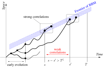
Figure 1. Leaders and their ancestors.

3. Almost sure convergence of the conditional maximum

We start with some elementary facts that will be of importance. First, observe that for $t,s>0$ such that $s=o(t)$ for $t\uparrow\infty$, the level of the maximum (1.4) satisfies

$$m(t) =m(t-s)+\sqrt{2}s+\frac{3}{2\sqrt{2}}\ln\left(\frac{t-s}{t}\right)$$ (3.1)

$$=m(t-s)+\sqrt{2}s+o(1).$$

Second, let $\{x_{j}(s),j\leq n(s)\}$ and, for $j=1\dots n(s)$, $\{x_{k}^{(j)}(t-s),k\leq n^{(j)}(t-s)\}$ be all independent, identically distributed BBMs. The Markov property of BBM implies

$$\{x_{k}(t),k\leq n(t)\}\stackrel{{\scriptstyle(d)}}{{=}}\{x_{j}(s)+x_{k}^{(j)}(t-s),j\leq n(s),\,k\leq n^{(j)}(t-s)\},$$ (3.2)

In particular, if $\mathcal{F}_{s}$ denotes the $\sigma$-algebra generated by the process up to time $s$, the combinination of (3.1) and (3.2) yields for $X\in\mathbb{R}$

$$\mathbb{P}\left[\forall_{k\leq n(t)}:\;\overline{x_{k}(t)}\leq X\mid\mathcal{F}_{s}\right]=\prod_{k\leq n(s)}\mathbb{P}\left[\forall_{j\leq n(t-s)}:\;\overline{x_{j}(t-s)}\leq X+y_{k}(s)+o(1)\mid\mathcal{F}_{s}\right]\ .$$ (3.3)

We will typically deal with situations where only a subset of $\{k:\,k=1,\dots,n(t)\}$ appears. In all such cases, the generalization of (3.3) is straightforward.

A key ingredient to the proof of Theorem 2 is a precise estimate on the right-tail of the distribution of the maximal displacement. It is related to [4, Proposition 3.3], which heavily relies on the work by Bramson [11].

Lemma 4.

Consider $t\geq 0$ and $X(t)\geq 0$ such that $\lim_{t\uparrow\infty}X(t)=+\infty$ and $X(t)=o(\sqrt{t})$ in the considered limit. Then, for $X(t)$ and $t$ both greater than $8r$,

$$C\gamma(r)^{-1}X(t)e^{-\sqrt{2}X(t)}\left(1-\frac{X(t)}{t-r}\right)\leq\mathbb{P}\left[M(t)\geq X(t)\right]\leq C\gamma(r)X(t)e^{-\sqrt{2}X(t)}$$ (3.4)

for some $\gamma(r)\downarrow 1$ as $r\to\infty$ and $C$ as in (1.12).

Proof.

Let us denote by $\overline{u}(t,x)\equiv 1-u(t,x)$, with $u$ the distribution of the maximal displacement defined in (1.1). We define

$$\psi(r,t,x+\sqrt{2}t)\equiv\frac{e^{-\sqrt{2}x}}{\sqrt{t-r}}\int_{0}^{\infty}\frac{dy^{\prime}}{\sqrt{2\pi}}\cdot\overline{u}(r,y^{\prime}+\sqrt{2}r)\cdot e^{y^{\prime}\sqrt{2}}\times$$ (3.5)

$$\hskip 56.9055pt\times\left\{1-\exp\left(-2y^{\prime}\frac{x+\frac{3}{2\sqrt{2}}\ln t}{t-r}\right)\right\}\exp\left(-\frac{(y^{\prime}-x)^{2}}{2(t-r)}\right).$$

According to [4, Proposition 3.3], for $r$ large enough, $t\geq 8r$, and $x\geq 8r-\frac{3}{2\sqrt{2}}\ln(t)$, the following bounds hold:

$$\gamma(r)^{-1}\psi(r,t,x+\sqrt{2}t)\leq\overline{u}(t,x+\sqrt{2}t)\leq\gamma(r)\psi(r,t,x+\sqrt{2}t)$$ (3.6)

for some $\gamma(r)\downarrow 1$ as $r\to\infty$.

As $\sqrt{2}t=m(t)+\frac{3}{2\sqrt{2}}\ln(t)$, by putting $\overline{x}\equiv x+\frac{3}{2\sqrt{2}}\ln(t)$, we reformulate the above as

$$\gamma(r)^{-1}\psi(r,t,\overline{x}+m(t))\leq\overline{u}(t,\overline{x}+m(t))\leq\gamma(r)\psi(r,t,\overline{x}+m(t)).$$ (3.7)

(The bounds in (3.7) hold for $\overline{x}\geq 8r$).

We lighten notations by setting

$$G(t,r;\overline{x},y^{\prime})\equiv\overline{u}(r,y^{\prime}+\sqrt{2}r)\cdot e^{y^{\prime}\sqrt{2}}\cdot\exp\left(-\frac{(y^{\prime}-\overline{x}+\frac{3}{2\sqrt{2}}\ln t)^{2}}{2(t-r)}\right),$$ (3.8)

and rewrite (3.7) accordingly:

$$\psi(r,t,\overline{x}+m(t)) =\frac{t^{3/2}e^{-\overline{x}\sqrt{2}}}{\sqrt{t-r}}\int_{0}^{\infty}\frac{dy^{\prime}}{\sqrt{2\pi}}\cdot\left\{1-e^{-2y^{\prime}\frac{\overline{x}}{t-r}}\right\}\cdot G(t,r;\overline{x},y^{\prime})$$ (3.9)

$$=t(1+o(1))e^{-\overline{x}\sqrt{2}}\int_{0}^{\infty}\frac{dy^{\prime}}{\sqrt{2\pi}}\cdot\left\{1-e^{-2y^{\prime}\frac{\overline{x}}{t-r}}\right\}\cdot G(t,r;\overline{x},y^{\prime}).$$

By a dominated convergence argument [11, Prop. 8.3 and its proof] one can prove that

$$C(r)\equiv\lim_{t\to\infty}\int_{0}^{\infty}2y^{\prime}G(t,r;\overline{x},y^{\prime})\frac{dy^{\prime}}{\sqrt{2\pi}},$$ (3.10)

exists, uniformly for $\overline{x}$ in compacts. In fact, Bramson’s argument easily extends to the case where $\overline{x}=o(\sqrt{t})$ (to see this, one simply expands the quadratic term in the Gaussian density appearing in the definition of the function $G$). Moreover, $C(r)\to C$ as $r\to\infty$, with $C$ as in (1.12), see [11, p. 145-146]. By Taylor expansion,

$$2y^{\prime}\frac{\overline{x}}{t-r}-\frac{2(y^{\prime})^{2}\overline{x}^{2}}{(t-r)^{2}}+\frac{f(t,r;x,y^{\prime})}{(t-r)^{3}}\leq\left\{1-e^{-2y^{\prime}\frac{\overline{x}}{t-r}}\right\}\leq 2y^{\prime}\frac{\overline{x}}{t-r}\,,$$ (3.11)

for some function $f(t,r;x,y^{\prime})$ which is integrable with respect to $G(t,r;\overline{x},y^{\prime})dy^{\prime}$.

Plugging (3.11) in (3.9) we get the bounds

$$\overline{u}(t,\overline{x}+m(t))\quad\geq \quad\overline{x}e^{-\overline{x}\sqrt{2}}\int_{0}^{\infty}2y^{\prime}G(t,r;\overline{x},y^{\prime})\frac{dy^{\prime}}{\sqrt{2\pi}}+$$ (3.12)

$$\hskip 56.9055pt+\frac{\overline{x}^{2}e^{-\overline{x}\sqrt{2}}}{t-r}\int_{0}^{\infty}2(y^{\prime})^{2}G(t,r;\overline{x},y^{\prime})\frac{dy^{\prime}}{\sqrt{2\pi}}+O((t-r)^{-2}),$$

$$\overline{u}(t,\overline{x}+m(t))\quad\leq \quad\overline{x}e^{-\overline{x}\sqrt{2}}\int_{0}^{\infty}2y^{\prime}G(t,r;\overline{x},y^{\prime})\frac{dy^{\prime}}{\sqrt{2\pi}},$$

for large enough $t$.

The claim of the Lemma then follows by taking $\overline{x}\equiv X(t)$ in (3.12) and using(3.10).

∎

Proof of Theorem 2.

This is a straightforward application of Lemma 4 and the convergence of the derivative martingale. First we write

$$\mathbb{P}\left[M(T\cdot s)\in\mathcal{D}\mid\mathcal{F}_{R_{T}}\right]=\mathbb{P}\left[M(T\cdot s)\leq D\mid\mathcal{F}_{R_{T}}\right]-\mathbb{P}\left[M(T\cdot s)\leq d\mid\mathcal{F}_{R_{T}}\right].$$ (3.13)

We will prove almost sure convergence of the first term, the second being identical. Since $s$ is in $(\varepsilon,1)$, we have $R_{T}=o(T\cdot s)$ for $T\uparrow\infty$. Therefore, by (3.1) and (3.2), and writing $\mathbb{P}_{M}$ for integration with respect to the maximum,

$$\mathbb{P}\left[M(T\cdot s)\leq D\mid\mathcal{F}_{R_{T}}\right]=$$ (3.14)

$$\quad=\prod_{k\leq n(R_{T})}\mathbb{P}_{M}\left[M(Ts-R_{T})\leq D+y_{k}(R_{T})\mid\mathcal{F}_{R_{T}}\right]$$

$$\quad=\prod_{k\leq n(R_{T})}\left\{1-\mathbb{P}_{M}\left[M(Ts-R_{T})>D+y_{k}(R_{T})\mid\mathcal{F}_{R_{T}}\right]\right\}$$

$$\quad=\exp\left(\sum_{k\leq n(R_{T})}\ln\big{(}1-\mathbb{P}_{M}\left[M(Ts-R_{T})>D+y_{k}(R_{T})\right]\big{)}\right)$$

It immediately follows from the almost sure convergence of the derivative martingale that

$$\lim_{R_{T}\uparrow\infty}\min_{k\leq n(R_{T})}y_{k}(R_{T})=+\infty\text{ almost surely.}$$ (3.15)

We may therefore use Lemma 4 to establish upper- and lower bounds for the probability of the maximum being larger than $D+y_{k}(R_{T})$, precisely:

$$C\gamma(r)^{-1}\big{\{}D+y_{k}(R_{T})\big{\}}\exp\Big{\{}-\sqrt{2}(D+y_{k}(R_{T})\Big{\}}\leq$$ (3.16)

$$\hskip 56.9055pt\leq\mathbb{P}_{M}\left[M(Ts-R_{T})>D+y_{k}(R_{T})\right]\leq$$

$$\hskip 85.35826pt\leq C\gamma(r)\big{\{}D+y_{k}(R_{T})\big{\}}\exp\Big{\{}-\sqrt{2}(D+y_{k}(R_{T})\Big{\}}\left(1+\frac{(D+y_{k}(R_{T}))}{Ts-R_{T}-r}\right),$$

for $Ts-R_{T}\geq 8r>0$.

The main contribution to both bounds above comes from the $z_{k}$-terms defined in (1.7). Precisely, we write (LABEL:gamma) as

$$C\gamma(r)^{-1}e^{-\sqrt{2}D}z_{k}(R_{T})+\omega_{k}(R_{T})\leq$$ (3.17)

$$\hskip 85.35826pt\leq\mathbb{P}_{M}\left[M(Ts-R_{T})>D+y_{k}(R_{T})\right]\leq$$

$$\hskip 142.26378pt\leq C\gamma(r)e^{-\sqrt{2}D}z_{k}(R_{T})+\Omega_{k}(R_{T})\ ,$$

where

$$\omega_{k}(R_{T}) \equiv C~{}D~{}\gamma(r)^{-1}e^{-\sqrt{2}D}e^{-\sqrt{2}y_{k}(R_{T})},$$ (3.18)

$$\Omega_{k}(R_{T}) \equiv C~{}D~{}\gamma(r)\left(1+\frac{(D+y_{k}(R_{T}))}{Ts-R_{T}-r}\right)\cdot e^{-\sqrt{2}D}e^{-\sqrt{2}y_{k}(R_{T})}\ .$$

By (LABEL:gamma_two), using that $-a\leq\ln(1-a)\leq-a+a^{2}/2$ (valid for $0<a<1/2$), and with the above notations, we obtain

$$\exp\left(-C\gamma(r)^{-1}e^{-\sqrt{2}D}Z(R_{T})-\sum_{k\leq n(R_{T})}\omega_{k}(R_{T})\right)$$ (3.19)

$$\hskip 56.9055pt\leq\mathbb{P}\left[M(T\cdot s)\leq D\mid\mathcal{F}_{R_{T}}\right]\leq$$

$$\exp\left(-C\gamma(r)e^{-\sqrt{2}D}Z(R_{T})+\frac{C^{2}}{2}\gamma(r)^{2}e^{-2\sqrt{2}D}Z^{(2)}(R_{T})+\sum_{k\leq n(R_{T})}(-\Omega_{k}(R_{T})+\frac{\Omega_{k}(R_{T})^{2}}{2})\right).$$

where $Z^{(2)}(R_{T})\equiv\sum_{k\leq n(R_{T})}y_{k}(R_{T})^{2}e^{-2\sqrt{2}y_{k}(R_{T})}$. To see that the $\omega$ terms in the lower bound do not contribute in the limit $T\uparrow\infty$ (recall that $R_{T}\uparrow\infty$ as well), we observe that for some $\kappa>0$ large enough and $Y(R_{T})$ as in (1.8),

$$\sum_{k\leq n(R_{T})}\omega_{k}(R_{T})\leq\kappa\cdot Y(R_{T})\to 0\text{ almost surely,}$$ (3.20)

by (1.9). Therefore the $\omega$ term in the lower bound do not contribute in the limit $T\uparrow\infty$.

Concerning the upper bound, the same argument as for the $\omega$ term together with the fact that $Z(R_{T})\to Z$ as $T\to\infty$ by (1.9) imply that

$$\sum_{k\leq n(R_{T})}\Omega_{k}(R_{T})\to 0\text{ almost surely.}$$ (3.21)

The same is thus also true for $\sum_{k\leq n(R_{T})}\Omega_{k}(R_{T})^{2}$. It remains to show that $Z^{(2)}(R_{T})\to 0$ almost surely, but this is evident since this sum is bounded from above by

$$\max_{k\leq n(R_{T})}\left(y_{k}(R_{T})^{2}e^{-\sqrt{2}y_{k}(R_{T})}\right)\times Y(R_{T}),$$ (3.22)

and both terms tend to zero, a.s., as $T\uparrow\infty$ by (3.15) and (1.9). Therefore, by (LABEL:conv_con_max_both),

$$\lim_{T\uparrow\infty}\mathbb{P}\left[M(T\cdot s)\leq D\mid\mathcal{F}_{R_{T}}\right]=\exp\left(-CZe^{-\sqrt{2}D}\right)\text{ almost surely.}$$ (3.23)

This concludes the proof of Theorem 2. ∎

4. The strong law of large numbers

This section is organized as follows. We introduce in subsection 4.1 a procedure concerning properties of the paths of extremal particles which we will refer to as localization. It is based on the description of the genealogies of extremal particles established in [2]. The details of the proof are given in subsection 4.2.

4.1. Preliminaries and localization of the paths

The following fundamental result by Bramson provides bounds to the right tail of the maximal displacement. These bounds are not optimal (they are surpassed by those of Lemma 4, which are tight), but they are sufficient and simpler.

Lemma 5.

[10, Section 5] Consider a branching Brownian motion $\{x_{j}(t)\}_{j\leq n(t)}$. Then, for $0\leq y\leq t^{1/2}$ and $t\geq 2$,

$$\mathbb{P}\left[\max_{j\leq n(t)}x_{j}(t)-m(t)\geq y\right]\leq\gamma(y+1)^{2}e^{-\sqrt{2}y},$$ (4.1)

where $\gamma$ is independent of $t$ and $y$.

We also recall an important property of the paths of extremal particles established by the authors in [2]. We introduce some notation. With $t\in\mathbb{R}_{+}$ and $\gamma>0$, we define

$$f_{\gamma,t}(s)\equiv\begin{cases}s^{\gamma}&0\leq s\leq t/2,\\ (t-s)^{\gamma}&t/2\leq s\leq t.\end{cases}$$ (4.2)

We now choose values

$$0<\alpha<1/2<\beta<1,$$ (4.3)

and introduce the time-$t$ entropic envelope, and the time-$t$ lower envelope respectively:

$$F_{\alpha,t}(s)\equiv\frac{s}{t}m(t)-f_{\alpha,t}(s),\quad 0\leq s\leq t,$$ (4.4)

and

$$F_{\beta,t}(s)\equiv\frac{s}{t}m(t)-f_{\beta,t}(s),\quad 0\leq s\leq t.$$ (4.5)

($m(t)$ is the level of the maximum of a BBM of length $t$). By definition,

$$F_{\beta,t}(s)<F_{\alpha,t}(s),$$ (4.6)

and

$$F_{\beta,t}(0)=F_{\alpha,t}(0)=0,\quad F_{\beta,t}(t)=F_{\alpha,t}(t)=m(t).$$ (4.7)

The space/time region between the entropic and lower envelopes will be denoted throughout as the time-t tube, or simply the tube.

By a slight abuse of notation, given a particle $k\leq n(t)$ which is at position $x_{k}(t)$ at time $t$, we refer to its path as $x_{k}(s)$ where $0\leq s\leq t$. Moreover, we will say that a particle $k$ is localized in the time $t$-tube during the interval $(r,t-r)$ if and only if

$$F_{\beta,t}(s)\leq x_{k}(s)\leq F_{\alpha,t}(s),\forall s\in(r,t-r)\ .$$

We say that it is not localized if the above requirement fails for some $s$ in $(r,t-r)$. The following proposition gives strong bounds to the probability of finding particles that are close to the level of the maximum at given times but not localized. It follows directly from the bounds derived in the course of the proof of [2, Corollary 2.6], cf. equations (5.5), (5.54), (5.62) and (5.63).

Proposition 6.

Let the subset $\mathcal{D}=[d,D]$ be given, with $-\infty<d<D\leq\infty$. There exist $r_{o},\delta>0$ depending on $\alpha,\beta$ and $\mathcal{D}$ such that

$$\sup_{t\geq 3r_{o}}\mathbb{P}\big{[}\exists_{k\leq n(t)}\,\overline{x_{k}(t)}\in\mathcal{D}\;\text{but the path is not}$$ (4.8)

$$\hskip 85.35826pt\text{localized in the time-$t$ tube during}\;(r,t-r)\big{]}\leq\exp\left(-r^{\delta}\right).$$

What lies behind the Proposition is a phenomenon of ”energy vs. entropy” which is absolutely fundamental for the whole picture. This is explained in detail in [2], but, for the reader’s convenience, we briefly sketch the argument.

As it turns out, at any given time $s\in(r,t-r)$ well inside the lifespan of a BBM, there are simply not enough particles lying above the entropic envelope for their offspring to make the jumps which eventually bring them to the edge at time $t$. On the other hand, although there are plenty of ancestors lying below the lower envelope, their position is so low that again none of their offspring will make it to the edge at time $t$. A delicate balance between number and positions of ancestors has to be met, and this feature is fully captured by the tubes.

With $\delta=\delta(\alpha,\beta,\mathcal{D})$ as in Proposition 6 we define

$$r_{T}\equiv(20\ln T)^{1/\delta}\ .$$ (4.9)

We now consider the maximum of the particles at time $s$ that are also localized during the interval $(r_{T},s-r_{T})$, see Figure 2 for a graphical representation. We denote this maximum by $M_{\text{loc}}(s)$.

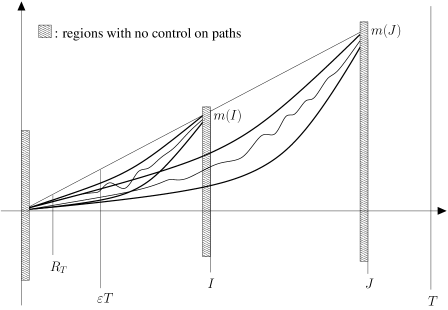
Figure 2. Maxima at different times $I,J$ are localized.

With this notation, by Proposition 6 and the choice (4.9),

$$0\leq\mathbb{P}\left[M(s)\in\mathcal{D}\right]-\mathbb{P}\left[M_{\text{loc}}(s)\in\mathcal{D}\right]\leq\frac{1}{T^{20}}.$$ (4.10)

We pick $R_{T}\equiv 40\cdot r_{T}$, with $r_{T}$ as in (4.9). This choice clearly satisfies $R_{T}=o(\sqrt{T})$ as required in Theorem 2. We emphasize that the prefactor is a choice. Only the condition $R_{T}>r_{T}$ is needed.

We assume henceforth without loss of generality that both $T$ and $\varepsilon T$ are integers.

4.2. Implementing the strategy

Recall that Theorem 3 asserts that

$$\text{Rest}_{\varepsilon,\mathcal{D}}(T)\equiv\frac{1}{T}\int_{\varepsilon T}^{T}\Big{(}\mathbbm{1}\{M(s)\in\mathcal{D}\}-\mathbb{P}\left[M(s)\in\mathcal{D}\mid\mathcal{F}_{R_{T}}\right]\Big{)}ds$$ (4.11)

tends to zero as $T$ goes to $\infty$. In order to prove the claim, we consider $\text{Rest}^{\text{loc}}_{\varepsilon,\mathcal{D}}(T)$, defined as $\text{Rest}_{\varepsilon,\mathcal{D}}(T)$ but with the requirement that all particles in $\mathcal{D}$ are localized:

$$\text{Rest}^{\text{loc}}_{\varepsilon,\mathcal{D}}(T)\equiv\frac{1}{T}\int_{\varepsilon T}^{T}\Big{(}\mathbbm{1}\{M_{\text{loc}}(s)\in\mathcal{D}\}-\mathbb{P}\left[M_{\text{loc}}(s)\in\mathcal{D}\mid\mathcal{F}_{R_{T}}\right]\Big{)}ds\ .$$ (4.12)

We now claim that the large $T$-limit of $\text{Rest}^{\text{loc}}_{\varepsilon,\mathcal{D}}(T)$ and that of $\text{Rest}_{\varepsilon,\mathcal{D}}(T)$ coincide (provided one of the two exists, but this will become apparent below).

Lemma 7.

With the above notation,

$$\lim_{T\uparrow\infty}\Big{(}\emph{Rest}_{\varepsilon,\mathcal{D}}(T)-\emph{Rest}^{\emph{loc}}_{\varepsilon,\mathcal{D}}(T)\Big{)}=0\text{ almost surely. }$$ (4.13)

Proof of Lemma 7.

We have

$$\text{Rest}_{\varepsilon,\mathcal{D}}(T)-\text{Rest}^{\text{loc}}_{\varepsilon,\mathcal{D}}(T)=$$ (4.14)

$$=\frac{1}{T}\int_{\varepsilon T}^{T}\Big{(}\mathbbm{1}\{M(s)\in\mathcal{D}\}-\mathbbm{1}\{M_{\text{loc}}(s)\in\mathcal{D}\}\Big{)}ds$$

$$\qquad-\frac{1}{T}\int_{\varepsilon T}^{T}\Big{(}\mathbb{P}\left[M(s)\in\mathcal{D}\mid\mathcal{F}_{R_{T}}\right]-\mathbb{P}\left[M_{\text{loc}}(s)\in\mathcal{D}\mid\mathcal{F}_{R_{T}}\right]\Big{)}ds$$

$$\equiv\boldsymbol{(1)_{T,\varepsilon}}-\boldsymbol{(2)_{T,\varepsilon}}.$$

The proof that $\lim_{T\uparrow\infty}\boldsymbol{(1)_{T,\varepsilon}}=0$ and $\lim_{T\uparrow\infty}\boldsymbol{(2)_{T,\varepsilon}}=0$ (almost surely) is identical and relies on an application of the Borel-Cantelli lemma. We thus prove only the first limit. Let $\epsilon>0$. By the Chebeychev inequality,

$$\mathbb{P}\left[\boldsymbol{(1)_{T,\varepsilon}}>\epsilon\right]\leq\frac{1}{T\epsilon}\int_{\varepsilon T}^{T}\Big{(}\mathbb{P}\left[M(s)\in\mathcal{D}\right]-\mathbb{P}\left[M_{\text{loc}}(s)\in\mathcal{D}\right]\Big{)}ds\leq$$ (4.15)

$$\stackrel{{\scriptstyle\eqref{bc}}}{{\leq}}\frac{1-\varepsilon}{\epsilon}T^{-20},$$

which is summable in $T$ (recalling that we assume $T\in\mathbb{N}$). Therefore, by Borel-Cantelli,

$$\mathbb{P}\left[\{\boldsymbol{(1)_{T,\varepsilon}}>\epsilon\}\;\text{infinitely often}\right]=0.$$ (4.16)

As the above holds for all $\epsilon>0$ we have that $\boldsymbol{(1)_{T,\varepsilon}}$ converges to $0$ as $T\uparrow\infty$ almost surely, and concludes the proof of Lemma 7. ∎

The following result is the major tool to establish the SLLN for the term $\text{Rest}^{\text{loc}}_{\varepsilon,\mathcal{D}}(T)$. (By Lemma 7, this will then imply that the same is true for $\text{Rest}_{\varepsilon,\mathcal{D}}(T)$). The result is a small extension of a theorem of Lyons [26, Theorem 1], where the statement is given for the sum of random variables.

Theorem 8.

Consider a process $\{X_{s}\}_{s\in\mathbb{R}_{+}}$ such that ${\mathbb{E}}[X_{s}]=0$ for all $s$. Assume furthermore that the random variables are uniformly bounded, say $\sup_{s}|X_{s}|\leq 2$ almost surely. If

$$\sum_{T=1}^{\infty}\frac{1}{T}{\mathbb{E}}\Big{[}\Big{|}\frac{1}{T}\int_{0}^{T}X_{s}~{}ds\Big{|}^{2}\Big{]}<\infty,$$ (4.17)

then

$$\lim_{T\to\infty}\frac{1}{T}\int_{0}^{T}X_{s}~{}ds=0,\text{ almost surely.}$$ (4.18)

Proof.

The extension to integrals is straightforward. In fact, by the summability assumption, we can find a subsequence $T_{k}\in\mathbb{N}$ of times such that

$$\sum_{k=1}^{\infty}{\mathbb{E}}\Big{[}\Big{|}\frac{1}{T_{k}}\int_{0}^{T_{k}}X_{t}~{}dt\Big{|}^{2}\Big{]}<\infty$$ (4.19)

where $T_{k}\to\infty$ and $T_{k+1}/T_{k}\to 1$. (See [26, Lemma 2]). Therefore by Fubini, the sum without the expectation is almost surely finite, and we must have

$$\lim_{k\to\infty}\frac{1}{T_{k}}\int_{0}^{T_{k}}X_{t}~{}dt\to 0\text{ almost surely .}$$ (4.20)

It remains to show this is true for all $T\in\mathbb{N}$. This is easy since the variables are bounded. For any $T$, there exists $k$ such that $T_{k}\leq T\leq T_{k+1}$. Thus

$$\Big{|}\frac{1}{T}\int_{0}^{T}X_{t}~{}dt\Big{|}\leq\Big{|}\frac{1}{T_{k}}\int_{0}^{T_{k}}X_{t}~{}dt\Big{|}+\max_{1\leq s\leq T_{k+1}-T_{k}}\Big{|}\frac{1}{T_{k}}\int_{T_{k}}^{T_{k}+s}X_{t}~{}dt\Big{|}\ .$$ (4.21)

The first term goes to zero by the previous argument. The second term goes to zero since

$$\max_{1\leq s\leq T_{k+1}-T_{k}}\Big{|}\frac{1}{T_{k}}\int_{T_{k}}^{T_{k}+s}X_{t}~{}dt\Big{|}\leq\frac{T_{K+1}-T_{k}}{T_{k}}\ ,$$ (4.22)

and $T_{k+1}/T_{k}\to 1$. ∎

Note that

$$\text{Rest}^{\text{loc}}_{\varepsilon,\mathcal{D}}(T) =\frac{1}{T}\int_{\varepsilon T}^{T}\Big{(}\mathbbm{1}\{M_{\text{loc}}(s)\leq D\}-\mathbb{P}\left[M_{\text{loc}}(s)\leq D\mid\mathcal{F}_{R_{T}}\right]\Big{)}ds$$ (4.23)

$$\qquad-\frac{1}{T}\int_{\varepsilon T}^{T}\Big{(}\mathbbm{1}\{M_{\text{loc}}(s)\leq d\}-\mathbb{P}\left[M_{\text{loc}}(s)\leq d\mid\mathcal{F}_{R_{T}}\right]\Big{)}ds$$

$$\equiv\frac{1}{T}\int_{\varepsilon T}^{T}X_{s}^{\{D\}}ds-\frac{1}{T}\int_{\varepsilon T}^{T}X_{s}^{\{d\}}ds,$$

with obvious notations. The goal is thus to prove that both integrals satisfy the assumptions of Theorem 8. We address the first integral, the proof for the second being identical. By construction, $\big{|}X_{s}^{\{D\}}\big{|}\leq 2$ a.s. for all $s$, and

$${\mathbb{E}}\left[X_{s}^{\{D\}}\right]=0\ .$$ (4.24)

It therefore suffices to check the assumption concerning the summability of correlations. Let

$$\widehat{C}_{T}(s,s^{\prime})\equiv{\mathbb{E}}\left[X_{s}^{(D)}\cdot X_{s^{\prime}}^{(D)}\right],$$ (4.25)

Note that by the properties of conditional expectation

$$\widehat{C}_{T}(s,s^{\prime}) ={\mathbb{E}}\Bigg{[}\Big{(}\mathbbm{1}\{M_{\text{loc}}(s)\leq D\}-\mathbb{P}\left[M_{\text{loc}}(s)\leq D\mid\mathcal{F}_{R_{T}}\right]\Big{)}\times$$ (4.26)

$$\hskip 56.9055pt\times\Big{(}\mathbbm{1}\{M_{\text{loc}}(s^{\prime})\leq D\}-\mathbb{P}\left[M_{\text{loc}}(s^{\prime})\leq D\mid\mathcal{F}_{R_{T}}\right]\Big{)}\Bigg{]}$$

$$={\mathbb{E}}\Bigg{[}\Bigg{(}\mathbb{P}\left[M_{\text{loc}}(s)\leq D,M_{\text{loc}}(s^{\prime})\leq D\mid\mathcal{F}_{R_{T}}\right]$$

$$\hskip 56.9055pt-\mathbb{P}\left[M_{\text{loc}}(s)\leq D\mid\mathcal{F}_{R_{T}}\right]\times\mathbb{P}\left[M_{\text{loc}}(s^{\prime})\leq D\mid\mathcal{F}_{R_{T}}\right]\Bigg{)}\Bigg{]}.$$

We claim that

$$\sum_{T}\frac{1}{T}{\mathbb{E}}\left[\Big{|}\frac{1}{T}\int_{\varepsilon T}^{T}X_{s}^{(D)}~{}ds\Big{|}^{2}\right]=2\sum_{T}\frac{1}{T^{3}}\int_{\varepsilon T}^{T}ds\int_{s}^{T}ds^{\prime}\widehat{C}_{T}(s,s^{\prime})\text{ is finite.}$$ (4.27)

In order to see this, and proceeding with the program outlined at the end of Section 2, we now specify the concept of times well separated from each other. Choose $0<\xi<1$ and split the integration according to the distance between $s$ and $s^{\prime}$:

$$\frac{1}{T^{3}}\int_{\varepsilon T}^{T}ds\int_{s}^{T}ds^{\prime}(\cdot)=\frac{1}{T^{3}}\int_{\varepsilon T}^{T}ds\int_{s}^{s+T^{\xi}}ds^{\prime}(\cdot)+\frac{1}{T^{3}}\int_{\varepsilon T}^{T}ds\int_{s+T^{\xi}}^{T}ds^{\prime}(\cdot).$$ (4.28)

The contribution of the first term on the r.h.s. above is negligible due to the uniform boundedness of the integrand and to the choice $0<\xi<1$. We are thus left to prove that the contribution to (LABEL:summability_lyons_two) of the second term in (LABEL:summability_lyons_three) is finite. The following is the key estimate.

Theorem 9.

There exists a finite $T_{o}$ such that the following holds for $T\geq T_{o}$: for some $\epsilon_{1},\epsilon_{2}>0$ not depending on $T$ (but on the other underlying parameters), the bound

$$\widehat{C}_{T}(s,s^{\prime})\leq(\ln T)^{\epsilon_{1}}e^{-(\ln T)^{\epsilon_{2}}}$$ (4.29)

holds uniformly for all $s,s^{\prime}$ such that $\varepsilon T\leq s<s^{\prime}\leq T$ and $s^{\prime}-s>T^{\xi}$.

The estimate directly implies the desired summability of the second term in (LABEL:summability_lyons_three). This concludes the proof Theorem 3. The proof of the estimate is somewhat lengthy and done in the next section.

5. Uniform bounds for the correlations.

We use here $I$ and $J$ to denote the two times $s,s^{\prime}$ from the statement of Theorem 9.

$\widehat{C}_{T}(I,J)$ is the expectation of the random variable

$$\hat{c}_{T}(I,J)\equiv\mathbb{P}\left[M_{\text{loc}}(I)\leq D,M_{\text{loc}}(J)\leq D\mid\mathcal{F}_{R_{T}}\right]$$ (5.1)

$$\hskip 113.81102pt-\mathbb{P}\left[M_{\text{loc}}(I)\leq D\mid\mathcal{F}_{R_{T}}\right]\times\mathbb{P}\left[M_{\text{loc}}(J)\leq D\mid\mathcal{F}_{R_{T}}\right].$$

We rewrite these conditional probabilities using the Markov property of BBM, considering independent BBM’s starting at their respective position at time $R_{T}$ and shifting the time by $R_{T}$. This requires some additional notation. Take

$$I_{T}\equiv I-R_{T},J_{T}\equiv J-R_{T}\ ,$$

and note that $m(I)=m(I_{T})+\sqrt{2}I_{T}+o(1)$ as $T\uparrow\infty$. We consider the collection $\{y_{k}(R_{T})\equiv\sqrt{2}R_{T}-x_{k}(R_{T})\}_{k\leq n(R_{T})}$ where the $\{x_{k}(R_{T})\}$ are the position of the particles of the original BBM at time $R_{T}$. Let $\{\tilde{x}_{l}(J_{T}),l\leq n(J_{T})\}$ be a BBM starting at zero, of length $J_{T}$, and of law $\tilde{\mathbb{P}}$ independent of $\mathbb{P}$. We write $\tilde{M}_{\text{loc}}(J_{T})$ for the maximum shifted by $m(J_{T})$ of this collection, restricted to $l$’s satisfying

$$y_{k}(R_{T})+\frac{s^{\prime}}{J}m(J)-f_{\beta,J}(R_{T}+s^{\prime})\leq\tilde{x}_{l}(s^{\prime})\leq y_{k}(R_{T})+\frac{s^{\prime}}{J}m(J)-f_{\alpha,J}(R_{T}+s^{\prime})\ ,$$ (5.2)

for $0\leq s^{\prime}\leq J_{T}-r_{T}$ (the ”shifted” $J$-tube). Similarly, $\tilde{M}_{\text{loc}}(I_{T})$ is the maximum shifted by $m(I_{T})$ of the positions of the particles at time $I_{T}$ with the localization condition

$$y_{k}(R_{T})+\frac{s^{\prime}}{I}m(I)-f_{\beta,I}(R_{T}+s^{\prime})\leq\tilde{x}_{l}(s^{\prime})\leq y_{k}(R_{T})+\frac{s^{\prime}}{J}m(J)-f_{\alpha,J}(R_{T}+s^{\prime}),$$ (5.3)

for $0\leq s^{\prime}\leq I_{T}-r_{T}$ (the ”shifted” $I$-tube). Note that the localization depends on $k$ (in fact on $y_{k}(R_{T})$). We drop this dependence in the notation $\tilde{M}_{\text{loc}}$ for simplicity.

By the Markov property, the first conditional probability in $\hat{c}_{T}(I,J)$ can be written in terms of the shifted process just defined:

$$\mathbb{P}\left[M_{\text{loc}}(I)\leq D,M_{\text{loc}}(J)\leq D\mid\mathcal{F}_{R_{T}}\right]$$ (5.4)

$$=\prod^{\star}_{k\leq n(R_{T})}\tilde{\mathbb{P}}\left[\tilde{M}_{\text{loc}}(I_{T})\leq D+y_{k}(R_{T}),\tilde{M}_{\text{loc}}(J_{T})\leq D+y_{k}(R_{T})\right],$$

where the product runs over all the particles $k$’s at time $R_{T}$ whose path is localized in the intersection of the $I-$ and $J-$tubes during the interval $(r_{T},R_{T})$. The restriction to localized positions at time $R_{T}$ is weaker and sufficient for our purpose:

$$k=1\dots n(R_{T})\,\text{such that}\;y_{k}(R_{T})\in\left(R_{T}^{\alpha}+\Omega_{T},R_{T}^{\beta}+\Omega_{T}\right)\hskip 28.45274pt(\bigtriangleup).$$ (5.5)

(Here and henceforth, we will use $\Omega_{T}$ to denote a negligible term, which is not necessarily the same at different occurences. In the above case it holds $\Omega_{T}=O(\ln\ln T)$ by definition of the tubes). We thus get that (LABEL:c_one) is at most

$$\prod_{\bigtriangleup}\tilde{\mathbb{P}}\left[\tilde{M}_{\text{loc}}(I_{T})\leq D+y_{k}(R_{T}),\tilde{M}_{\text{loc}}(J_{T})\leq D+y_{k}(R_{T})\right]\ .$$ (5.6)

Let

$$\wp(I_{T};y_{k}(R_{T}))\equiv\tilde{\mathbb{P}}\left[\tilde{M}_{\text{loc}}(I_{T})>D+y_{k}(R_{T})\right],$$ (5.7)

(analogously for $J_{T}$) and

$$\wp(I_{T},J_{T};y_{k}(R_{T}))\equiv\tilde{\mathbb{P}}\left[\tilde{M}_{\text{loc}}(I_{N})>D+y_{k}(R_{T})\;\text{and}\;\tilde{M}_{\text{loc}}(J_{T})>D+y_{k}(R_{T})\right].$$ (5.8)

Finally, define

$$\widehat{Z}(\cdot;R_{T}) \equiv \sum_{\bigtriangleup}\wp(\cdot;y_{k}(R_{T})),$$ (5.9)

$$\mathcal{R}_{T} \equiv \frac{1}{2}\sum_{\bigtriangleup}\Big{\{}\wp(I_{T};y_{k}(R_{T}))+\wp(J_{T};y_{k}(R_{T}))-\wp(I_{T},J_{T};y_{k}(R_{T})\Big{\}}^{2}.$$ (5.10)

Proposition 10.

With the above definitions,

$$0\leq\hat{c}_{T}(I,J)\leq\widehat{Z}(I_{T},J_{T};R_{T})+\mathcal{R}_{T},$$ (5.11)

almost surely, for $T$ large enough.

Proof.

In the notation introduced above, one has

$$\prod_{\bigtriangleup}\tilde{\mathbb{P}}\left[\tilde{M}_{\text{loc}}(I_{T})\leq D+y_{k}(R_{T}),\tilde{M}_{\text{loc}}(J_{T})\leq D+y_{k}(R_{T})\right]$$ (5.12)

$$\qquad=\exp\left\{\sum_{\bigtriangleup}\ln\Big{[}1-\wp(I_{T};y_{k}(R_{T}))-\wp(J_{T};y_{k}(R_{T}))+\wp(I_{T};J_{T};y_{k}(R_{T}))\Big{]}\right\}\ .$$

Note that for all $k\in\bigtriangleup$

$$\wp(I_{T};y_{k}(R_{T}))\leq\tilde{\mathbb{P}}\left[\tilde{M}(I_{T})\geq D+y_{k}(R_{T})\right]\leq\gamma(1+y_{k}(R_{T})+D)^{2}e^{-\sqrt{2}(y_{k}(R_{T})+D)}\ .$$ (5.13)

The first inequality holds by dropping the localization condition. Therefore, this can be made arbitrarily small (uniformly in $k$) by choosing $T$ large enough. The same obviously holds for $\wp(J_{T};y_{k}(R_{T}))$ and $\wp(I_{T},J_{T};y_{k}(R_{T}))$. Choose $T$ large enough so that

$$\sup_{\bigtriangleup}\max\{\wp(I_{T};y_{k}(R_{T})),\wp(J_{T};y_{k}(R_{T})),\wp(I_{T},J_{T};y_{k}(R_{T}))\}\leq{1/6}.$$ (5.14)

Coming back to (LABEL:log_P), using that

$$-a\leq\ln(1-a)\leq-a+a^{2}/2\quad(0\leq a\leq 1/2),$$ (5.15)

(with $a\equiv\wp(I_{T};y_{k}(R_{T}))+\wp(J_{T};y_{k}(R_{T}))-\wp(I_{T};J_{T};y_{k}(R_{T}))$, for $k\in\bigtriangleup$), we get that (LABEL:log_P) is at most

$$\exp\Bigg{(}-\widehat{Z}(I_{T};R_{T})-\widehat{Z}(J_{T};R_{T})+\widehat{Z}(I_{T},J_{T};R_{T})+\mathcal{R}_{T}\Bigg{)}.$$ (5.16)

This is an upper bound for the first conditional probability in the definition of $\hat{c}_{T}(I,J)$. A similar reasoning, using this time the first inequality in (5.15), yields a lower bound for the second term in $\hat{c}_{T}(I,J)$, i,e, the product of the conditional probabilities. The upshot is:

$$\hat{c}_{T}(I,J)\leq e^{-\widehat{Z}(I_{T};R_{T})-\widehat{Z}(J_{T};R_{T})}\left\{e^{\widehat{Z}(I_{T},J_{T};R_{T})+\mathcal{R}_{T}}-1\right\},$$ (5.17)

almost surely and for large enough $T$. We now use that $e^{a}-1\leq a\cdot e^{a}$ (which holds for $a>0$) for the term in the brackets to get that (5.17) is at most

$$e^{-\widehat{Z}(I_{T};R_{T})-\widehat{Z}(J_{T};R_{T})}\left(\widehat{Z}(I_{T},J_{T};R_{T})+\mathcal{R}_{T}\right)\cdot e^{\widehat{Z}(I_{T},J_{T};R_{T})+\mathcal{R}_{T}}.$$ (5.18)

By construction, $\widehat{Z}(I_{T},J_{T};R_{T})\leq\min\left\{\widehat{Z}(I_{T};R_{T});\widehat{Z}(I_{T};R_{T})\right\}$, implying that

$$\widehat{Z}(I_{T},J_{T};R_{T})-\frac{1}{2}\widehat{Z}(I_{T};R_{T})-\frac{1}{2}\widehat{Z}(J_{T};R_{T})\leq 0,$$ (5.19)

and therefore (LABEL:c_eight) is at most

$$\left(\widehat{Z}(I_{T},J_{T};R_{T})+\mathcal{R}_{T}\right)\cdot e^{\mathcal{R}_{T}-\frac{1}{2}\widehat{Z}(I_{T};R_{T})-\frac{1}{2}\widehat{Z}(J_{T};R_{T})}.$$ (5.20)

This is not far from the claim of Proposition 10. It remains to get rid of the exponential on the r.h.s. above. Using the bound (5.26), together with the definition of the $\widehat{Z}$ and rearranging, we arrive at

$$\mathcal{R}_{T}-\frac{1}{2}\widehat{Z}(I_{T};R_{T})-\frac{1}{2}\widehat{Z}(J_{T};R_{T})$$ (5.21)

$$\quad\leq\sum_{\bigtriangleup}\wp(I_{T};y_{k}(R_{T}))\left(3\wp(I_{T};y_{k}(R_{T}))-\frac{1}{2}\right)$$

$$\hskip 113.81102pt+\sum_{\bigtriangleup}\wp(J_{T};y_{k}(R_{T}))\left(3\wp(J_{T};y_{k}(R_{T}))-\frac{1}{2}\right).$$

In view of (5.13), we may find $T$ large enough such that the following holds uniformly for all $k\in\bigtriangleup$:

$$3\wp(I_{T};y_{k}(R_{T}))-\frac{1}{2}\leq 0,\qquad 3\wp(J_{T};y_{k}(R_{T}))-\frac{1}{2}\leq 0,$$ (5.22)

in which case all terms appearing in (LABEL:getting_rid) become negative, and this implies that

$$\hat{c}_{T}(I,J)\leq\widehat{Z}(I_{T},J_{T};R_{T})+\mathcal{R}_{T},$$ (5.23)

concluding the proof of Proposition 10. ∎

5.1. Proof of Theorem 9

We first observe that the expectation of $\mathcal{R}_{T}$ appearing in Proposition 10 gives the right bound in Theorem 9. Indeed, using that $(a+b+c)^{2}\leq 4a^{2}+4b^{2}+4c^{2}$, we get the upper bound

$$\mathcal{R}_{T} =\frac{1}{2}\sum_{\bigtriangleup}\Big{\{}\wp(I_{T};y_{k}(R_{T}))+\wp(J_{T};y_{k}(R_{T}))-\wp(I_{T},J_{T};y_{k}(R_{T})\Big{\}}^{2}$$ (5.24)

$$\leq 2\sum_{\bigtriangleup}\wp(I_{T};y_{k}(R_{T}))^{2}+\wp(J_{T};y_{k}(R_{T}))^{2}+\wp(I_{T},J_{T};y_{k}(R_{T}))^{2}.$$

Moreover,

$$\wp(I_{T},J_{T};y_{k}(R_{T})) \leq\frac{1}{2}\wp(I_{T};y_{k}(R_{T}))+\frac{1}{2}\wp(J_{T};y_{k}(R_{T})).$$ (5.25)

Inserting this in (5.24), we get

$$\mathcal{R}_{T}\leq\sum_{\bigtriangleup}\left\{3\wp(I_{T};y_{k}(R_{T}))^{2}+3\wp(J_{T};y_{k}(R_{T}))^{2}\right\}.$$ (5.26)

By (5.26), (5.13) and (5.5), and for some irrelevant numerical constants $\kappa$,

$${\mathbb{E}}\left[\mathcal{R}_{T}\right] \leq\kappa{\mathbb{E}}\left[\sum_{\bigtriangleup}y_{k}(R_{T})^{2}e^{-2\sqrt{2}y_{k}(R_{T})}\right]$$ (5.27)

$$\leq\kappa e^{R_{T}}\int_{R_{T}^{\alpha}+\Omega_{T}}^{R_{T}^{\beta}+\Omega_{T}}y^{2}e^{-2\sqrt{2}y}e^{-\frac{(y-\sqrt{2}R_{T})^{2}}{2R_{T}}}\frac{dy}{\sqrt{2\pi R_{T}}}$$

$$\leq\kappa R_{T}^{2}e^{-\sqrt{2}R_{T}^{\alpha}}=\kappa(\ln T)^{2/\delta}e^{-\kappa(\ln T)^{\alpha/\delta}},$$

which is at most

$${\mathbb{E}}\left[\mathcal{R}_{T}\right]\leq(\ln T)^{\epsilon^{(1)}}e^{-(\ln T)^{\epsilon^{(2)}}},$$ (5.28)

for some $\epsilon^{(1)},\epsilon^{(2)}>0$. It will remain to prove that ${\mathbb{E}}[\widehat{Z}(I_{T},J_{T};R_{T})]$ behaves similarly to establish Theorem 9.

Recall that

$$\widehat{Z}(I_{T},J_{T};R_{T})=\sum_{\bigtriangleup}\wp(I_{T},J_{T};y_{k}(R_{T})),$$ (5.29)

and

$$\wp(I_{T},J_{T};y_{k}(R_{T}))=\tilde{\mathbb{P}}\left[\tilde{M}_{\text{loc}}(I_{T})>D+y_{k}(R_{T})\;\text{and}\;\tilde{M}_{\text{loc}}(J_{T})>D+y_{k}(R_{T})\right].$$ (5.30)

By definition, (5.30) is the probability to find a particle of the BBM which has two extremal descendants, particle $\boldsymbol{(1)}$ say, whose position is above $m(I_{T})+D+y_{k}(R_{T})$ at time $I_{T}$, and particle $\boldsymbol{(2)}$, which lies above $m(J_{T})+D+y_{k}(R_{T})$ at time $J_{T}$. These two particles also satisfy localization conditions on their paths. In other words, this is the probability that the same ancestor $k$, with (relative) position $y_{k}(R_{T})$, produces children $\boldsymbol{(1)}$ and $\boldsymbol{(2)}$ which are extremal at time $I$ and $J$. As these generations are well separated in time, that is $J-I>T^{\xi}$ (and thus also $J_{T}-I_{T}>T^{\xi}$), we may expect this probability to be very small.

In order to see that this is indeed the case, split the probabilities according to whether the most recent common ancestor of particles $\boldsymbol{(1)}$ and $\boldsymbol{(2)}$ has branched before time $I_{T}-r_{T}$ (with $r_{T}$ as in (4.9)), or after. We write this as

$$\wp(I_{T},J_{T};y_{k}(R_{T})) =\wp(I_{T},J_{T};y_{k}(R_{T});\text{split before}\,I_{T}-r_{T})$$

$$\hskip 56.9055pt+\wp(I_{T},J_{T};y_{k}(R_{T});\text{split after}\,I_{T}-r_{T}).$$

(Figure 3 illustrates the first case).

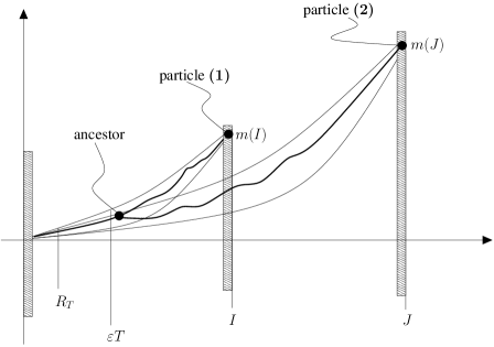
Figure 3. Time of branching before $I$

The second probability is in fact zero. Indeed, the condition (LABEL:cond_path_after_R_T) implies that the ancestor of $\boldsymbol{(2)}$ at time $I-r_{T}$ lies at heights which are at most the level of the entropic envelope associated with $J$. Since $J-I>T^{\xi}$ and this is easily seen to be way lower than the lower envelope of particle $\boldsymbol{(1)}$ associated with time $I$. In other words, the localization tubes of particles $\boldsymbol{(1)}$ and $\boldsymbol{(2)}$ are disjoint if their ancestor split after $I-r_{T}$. Hence, the splitting of the ancestor of particles $\boldsymbol{(1)}$ and $\boldsymbol{(2)}$ can only happen before time $I_{T}-r_{T}$:

$$\widehat{Z}(I_{T},J_{T};R_{T})=\sum_{\bigtriangleup}\wp(I_{T},J_{T};y_{k}(R_{T});\text{split before}\,I_{T}-r_{T})\text{ a.s.}$$ (5.31)

Proposition 11.

For some $\epsilon^{(3)},\epsilon^{(4)}>0$ and $T$ large enough the following bounds hold

$$\wp(I_{T},J_{T};y_{k}(R_{T});\text{split before}\,I_{T}-r_{T})$$ (5.32)

$$\qquad\leq(\ln T)^{\epsilon^{(3)}}e^{-(\ln T)^{\epsilon^{(4)}}}y_{k}(R_{T})e^{-\sqrt{2}(y_{k}(R_{T})},$$

uniformly for all $k\in\bigtriangleup$ and $I_{T},J_{T}$ as considered, almost surely.

The proof of this proposition is technical, and postponed to section 5.2. We show how this provides the last piece for the proof of Theorem 9. This is straightforward: by similar computations as in (5.27),

$${\mathbb{E}}\left[\sum_{k\in\bigtriangleup}y_{k}(R_{T})e^{-\sqrt{2}y_{k}(R_{T})}\right]\leq\kappa\cdot\sqrt{R_{T}}=\kappa\ln(T)^{1/2\delta},$$ (5.33)

for large enough $\kappa>0$ and recalling that by definition $R_{T}=40(\ln T)^{1/\delta}$. This, together with (LABEL:really_almost) implies

$${\mathbb{E}}\left[\sum_{k\in\bigtriangleup}\wp(I_{T},J_{T};y_{k}(R_{T});\text{split before}\,I_{T}-r_{T})\right]\leq\kappa(\ln T)^{\epsilon^{(3)}+1/2\delta}e^{-(\ln T)^{\epsilon^{(4)}}}.$$ (5.34)

Combining this with (5.28) we see that the claim of Theorem 9 holds with

$$\epsilon_{1}\equiv\max\left\{\epsilon^{(1)};\epsilon^{(3)}+1/2\delta\right\},$$ (5.35)

and

$$\epsilon_{2}\equiv\min\left\{\epsilon^{(2)};\epsilon^{(4)}\right\}.$$ (5.36)

$\square$

5.2. Proof of Proposition 11

The claim is that

$$\wp(I_{T},J_{T};y_{k}(R_{T});\text{split before}\,I_{T}-r_{T})$$ (5.37)

$$\qquad\leq(\ln T)^{\epsilon^{(3)}}e^{-(\ln T)^{\epsilon^{(4)}}}y_{k}(R_{T})e^{-\sqrt{2}y_{k}(R_{T})},$$

holds uniformly for $k\in\bigtriangleup$. In order to prove this, we use a formula by Sawyer [29] concerning the expected number of pairs of particles ancestor branched in the interval $(0,I_{T}-r_{T})$ and whose paths satisfy certain localization conditions, say $T^{(1)}$ and $T^{(2)}$ respectively. The expected number of such pairs is given by

$$Ke^{I_{T}}\int_{0}^{I_{T}-r_{T}}ds\cdot e^{J_{T}-s}\int d\mu_{s}(y)\mathbb{P}\left[x\in T^{(1)}_{(0,s)}\cap T^{(2)}_{(0,s)}\mid x(s)=y\right]\times$$ (5.38)

$$\times\mathbb{P}\left[x\in T^{(1)}_{(s,I_{T})}\mid x(s)=y\right]\times\mathbb{P}\left[x\in T_{(s,J_{T})}^{(2)}\mid x(s)=y\right].$$

Here the probability $\mathbb{P}$ is the law of a Brownian motion $x$, and $K=\sum_{j}p_{j}j(j-1)$ (with $\{p_{j}\}$ the offspring distribution). The time $s$ is the branching time of the common ancestor, and $\mu_{s}$ is the Gaussian measure with variance $s$. $T^{(\cdot)}_{(a,b)}$ denotes the condition on the path during the time interval $(a,b)$.

A proof of this formula is given in [29, p. 664 and 686]. Sawyer counts the pairs of particles for the same time, whereas our case concerns particles for two different times: particle $\boldsymbol{(1)}$ at time $I_{T}$, and particle $\boldsymbol{(2)}$ at time $J_{T}$. The generalization of Sawyer’s formula is however straightforward. The reader is referred to the intuitive construction of the formula provided by Bramson [10, p. 564].

Dropping the condition $T^{(2)}$ in the first probability of (LABEL:sawyer_general) yields a simpler bound:

$$\eqref{sawyer_general}\leq Ke^{I_{T}}\int_{0}^{I_{T}-r_{T}}ds\cdot e^{J_{T}-s}\int d\mu_{s}(y)\mathbb{P}\left[x\in T^{(1)}_{(0,I_{T})}\mid x(s)=y\right]\times$$ (5.39)

$$\hskip 170.71652pt\times\mathbb{P}\left[x\in T_{(s,J_{T})}^{(2)}\mid x(s)=y\right]\ .$$

Note that $\wp(I_{T},J_{T};y_{k}(R_{T});\text{split before}\,I_{T}-r_{T})$ is by Markov inequality at most the expected number of pairs $\{\boldsymbol{(1),(2)}\}$ of particles which satisfy their respective localization conditions with the common ancestor branching before time $I_{T}-r_{T}$. By (5.39), it thus holds:

$$\wp(I_{T},J_{T};y_{k}(R_{T});\text{split before}\,I_{T}-r_{T})$$ (5.40)

$$\qquad\leq Ke^{I_{T}}\int_{0}^{I_{T}-r_{T}}ds\cdot e^{J_{T}-s}\int d\mu_{s}(y)\mathbb{P}\left[x\in T^{(1)}_{(0,I_{T})}\mid x(s)=y\right]\times$$

$$\hskip 227.62204pt\times\mathbb{P}\left[x\in T_{(s,J_{T})}^{(2)}\mid x(s)=y\right]$$

with $T^{(1)}$ and $T^{(2)}$ being the shifted tubes defined in (LABEL:cond_path_after_R_T) and (LABEL:cond_path_after_R_T_two).

The idea is now to bound the second probability appearing in (LABEL:huckleberry) uniformly in $y$. This procedure has been introduced in Bramson [10, Lemma 11], and proved useful also in [2, Theorem 2.1].

Lemma 12.

It holds:

$$\mathbb{P}\left[x\in T_{(s,J_{T})}^{(2)}\mid x(s)=y\right]$$ (5.41)

$$\qquad\leq\Omega_{T}^{2}e^{-(J_{T}-s)}\exp\left(-\sqrt{2}f_{\alpha,J}(R_{T}+s)-\frac{3}{2}\ln\left(\frac{J_{T}-s}{J_{T}}\right)-\frac{3}{2}\frac{s}{J_{T}}\ln J_{T}\right),$$

where $\Omega_{T}=O((\ln T)^{1/2\delta})$ as $T\uparrow\infty$.

For the proof of Lemma 12 some facts concerning the Brownian bridge are needed. Denoting a standard Brownian motion by $x$, the Brownian bridge of length $t$ starting and ending at zero, is the Gaussian process

$$\mathfrak{z}_{t}(s)\equiv x(s)-\frac{s}{t}x(t),\qquad 0\leq s\leq t.$$ (5.42)

The Brownian bridge is a Markov process, and it has the property that $\mathfrak{z}_{t}(s),0\leq s\leq t$ is independent of $x(t)$. This construction generalizes to the case where the endpoints of the bridge are $a,b\neq 0$; we denote by $\mathfrak{z}_{t}^{(a,b)}(s)$ such a process. The following is also well known:

$$\mathfrak{z}_{t}^{(a,b)}(s)\stackrel{{\scriptstyle(d)}}{{=}}\mathfrak{z}_{t}(s)+\left(1-\frac{s}{t}\right)a+\left(\frac{s}{t}\right)b,\qquad 0\leq s\leq t,$$ (5.43)

with equality holding in distribution.

We now recall [2, Lemma 3.4] which deals with probabilities that a Brownian bridge stays below linear functions; the proof is elementary and will not be given here.

Lemma 13.

Let $z_{1},z_{2}\geq 0$ and $r_{1},r_{2}\geq 0$. Then for $t>r_{1}+r_{2}$,

$$\mathbb{P}\left[\mathfrak{z}_{t}(s)\leq\left(1-\frac{s}{t}\right)z_{1}+\frac{s}{t}z_{2},\,r_{1}\leq s\leq t-r_{2}\right]$$ (5.44)

$$\hskip 113.81102pt\leq\frac{2}{t-r_{1}-r_{2}}\prod_{i=1,2}\left\{z(r_{i})+\sqrt{r_{i}}\right\},$$

where $z(r_{1})\equiv\left(1-\frac{r_{1}}{t}\right)z_{1}+\frac{r_{1}}{t}z_{2}$ and $z(r_{2})\equiv\frac{r_{2}}{t}z_{1}+\left(1-\frac{r_{2}}{t}\right)z_{2}$.

Proof of Lemma 12.

We begin by first writing explicitly the underlying conditions on the paths. For $f:\mathbb{R}_{+}\to\mathbb{R},t\mapsto f(t)$ a generic function, we denote by $f^{S}(\cdot)\equiv f(S+\cdot)$ its time-shift by $S>0$. We also shorten $y(s)\equiv\sqrt{2}s-x(s)$, where $x(s)=y$ as in (LABEL:huckleberry), and $J_{T,s}\equiv J_{T}-s$. We also set $\Omega_{T}\equiv O(\ln\ln T)$. By elementary manipulations one easily sees that

$$\mathbb{P}\left[x\in T_{(s,J_{T})}^{(2)}\mid x(s)=y\right]=\mathbb{P}\left[\boldsymbol{(E)}\right],$$ (5.45)

where $\boldsymbol{(E)}$ is the event

$$\boldsymbol{(E)}=\begin{cases}x(J_{T,s})\geq m(J_{T,s})+y(s)+\frac{3}{2\sqrt{2}}\ln\left(\frac{J_{T,s}}{J_{T}}\right)+D+y_{k}(R_{T})+\Omega_{T}&\hfill\boldsymbol{(E_{1})}\\ F_{1}(t)\leq x(t)\leq F_{2}(t),\qquad 0\leq t\leq J_{T,s}-r_{T}&\hfill\boldsymbol{(E_{2})}\\ \end{cases}$$ (5.46)

where $F_{1},F_{2}$ are the entropic (resp. lower) envelopes of (LABEL:cond_path_after_R_T) shifted by $s$:

$$F_{1}(t) \equiv y_{k}(R_{T})+y(s)+\frac{t}{J_{T}}m(J_{T})+\frac{3}{2\sqrt{2}}\frac{s}{J_{T}}\ln(J_{T})-f_{\alpha,J}^{R_{T}+s}(t)+\Omega_{T},$$ (5.47)

$$F_{2}(t) \equiv y_{k}(R_{T})+y(s)+\frac{t}{J_{T}}m(J_{T})+\frac{3}{2\sqrt{2}}\frac{s}{J_{T}}\ln(J_{T})-f_{\beta,J}^{R_{T}+s}(t)+\Omega_{T},$$

with $\Omega_{T}=O(\ln\ln T)$. By the very same localizations, we also have a condition on $x(s)$. This reads

$$x(s) \in\Big{(}-f_{\beta,J}^{R_{T}}(s);-f_{\alpha,J}^{R_{T}}(s)\Big{)}+y_{k}(R_{T})+\sqrt{2}s-\frac{3}{2\sqrt{2}}\frac{s}{J_{T}}\ln(J_{T}).$$ (5.48)

For later use, we reformulate (5.48) into a condition on $y_{k}(R_{T})+y(s)$, namely:

$$y_{k}(R_{T})+y(s)\in\Big{(}f_{\alpha,J}^{R_{T}}(s);f_{\beta,J}^{R_{T}}(s)\Big{)}+\frac{3}{2\sqrt{2}}\frac{s}{J_{T}}\ln(J_{T}).$$ (5.49)

We now construct an event $\boldsymbol{(E^{\prime})}\supsetneq\boldsymbol{(E)}$. First, we drop the condition that the Brownian path is required to stay above $F_{2}$. Second, we replace the condition on $F_{1}$ by the condition that the $x$-path remains, on the interval $(0,J_{T,s}-r_{T})$, below the line segment interpolating between $(0,F_{1}(0))$ and $(J_{T,s},F_{1}(J_{T,s}))$, see Figure 4 for a graphical representation. Precisely, we consider

$$\boldsymbol{(E^{\prime})}=\begin{cases}x(J_{T,s})\geq m(J_{T,s})+y(s)+\frac{3}{2\sqrt{2}}\ln\left(\frac{J_{T,s}}{J_{T}}\right)+D+y_{k}(R_{T})+\Omega_{T}&\hfill\boldsymbol{(E^{\prime}_{1})}\\ x(t)\leq\left(1-\frac{t}{J_{T,s}}\right)F_{1}(0)+\frac{t}{J_{T,s}}F_{1}(J_{T,s})\qquad 0\leq t\leq J_{T,s}-r_{T}&\hfill\boldsymbol{(E^{\prime}_{2})}\\ \end{cases}$$ (5.50)

By construction,

$$\mathbb{P}\left[\boldsymbol{(E)}\right]\leq\mathbb{P}\left[\boldsymbol{(E^{\prime})}\right].$$ (5.51)

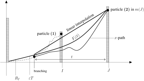
Figure 4. The $x$-path stays below the linear interpolation

Let us put

$$X(s,J_{T}) \equiv m(J_{T,s})+y(s)+\frac{3}{2\sqrt{2}}\ln\left(\frac{J_{T,s}}{J_{T}}\right)+D+y_{k}(R_{T})+\Omega_{T}$$ (5.52)

$$=\sqrt{2}J_{T,s}-\frac{3}{2\sqrt{2}}\ln J_{T,s}+\left\{\frac{3}{2\sqrt{2}}\ln\left(\frac{J_{T,s}}{J_{T}}\right)+y(s)+y_{k}(R_{T})+\Omega_{T}\right\}.$$

We write

$$\mathbb{P}\left[\boldsymbol{(E^{\prime})}\right] =\int_{0}^{\infty}\mathbb{P}\left[\boldsymbol{(E^{\prime}_{2})}\big{|}x(J_{T,s})=X(s,J_{T})+X\right]\tilde{\mu}(dX),$$ (5.53)

where $\tilde{\mu}$ is a Gaussian with variance $J_{T,s}$ and mean $-X(s,J_{T})$, i.e.

$$\tilde{\mu}(dX)=\exp\left(-\frac{(X+X(s,J_{T}))^{2}}{2J_{T,s}}\right)\frac{dX}{\sqrt{2\pi J_{T,s}}}\,.$$ (5.54)

We now make some observations concerning the Gaussian density and the conditional probability appearing in (5.53).

For the Gaussian density, we recall that $J_{T,s}=J_{T}-s$ for $0\leq s\leq I_{T}-r_{T}\leq I_{T}$. Moreover, since $J_{T}-I_{T}>T^{\xi}$ and $J_{T}\geq\varepsilon T$, we see that

$$-(1-\xi)\ln T-\ln\varepsilon\leq\ln\left(\frac{J_{T,s}}{J_{T}}\right)\leq 0.$$ (5.55)

And,

$$y(s)+y_{k}(R_{T})=o(J_{T,s})\quad(T\uparrow\infty),$$ (5.56)

by (5.49). Therefore, combining (5.55) and (5.56) we have that $X(s,J_{T})=\sqrt{2}J_{T,s}+o(J_{T,s})$ as $T\uparrow\infty$. The Gaussian density can thus be developed as follows

$$\tilde{\mu}(dX)=J_{T,s}e^{-J_{T,s}}e^{-\sqrt{2}\Delta_{T}(s)}g_{T}(X)dX,$$ (5.57)

where

$$\Delta_{T}(s)\equiv y(s)+\frac{3}{2\sqrt{2}}\ln\left(\frac{J_{T,s}}{J_{T}}\right)+y_{k}(R_{T}),$$ (5.58)

and

$$g_{T}(X)\equiv\frac{e^{-X^{2}/2J_{T,s}}}{\sqrt{2\pi}}e^{-\sqrt{2}(1+\omega_{T})X}\left(1+\Omega_{T}\right),$$ (5.59)

$\omega_{T}=o(1)$ as $T\uparrow\infty$, and $\Omega_{T}=O(\ln\ln T)$.

For the conditional probability appearing in (5.53), we observe that conditioning on the event $\{x(J_{T,s})=X\}$, turns the Brownian motion involved in the definition of $\boldsymbol{E^{\prime}_{2}}$ into a Brownian bridge ending at the conditioning point. Precisely,

$$\mathbb{P}\left[\boldsymbol{(E^{\prime}_{2})}\mid x(J_{T,s})=X(s,J_{T})+X\right]=\mathbb{P}\left[\boldsymbol{(E^{\prime\prime})}\right],$$ (5.60)

where

$$\boldsymbol{(E^{\prime\prime})} \equiv\Big{\{}\forall_{0\leq t\leq J_{T,s}-r_{T}}:\;\mathfrak{z}_{J_{T,s}}(t)\leq\left(1-\frac{t}{J_{T,s}}\right)F_{1}(0)+\frac{t}{J_{T,s}}\left(F_{1}(J_{T,s})-X(s,J_{T})-X\right)\Big{\}}$$ (5.61)

$$\quad=\Big{\{}\forall_{0\leq t\leq J_{T,s}-r_{T}}:\;\mathfrak{z}_{J_{T,s}}(t)\leq\left(1-\frac{t}{J_{T,s}}\right)F_{1}(0)+\frac{t}{J_{T,s}}\left(\Omega_{T}-X\right)\Big{\}},$$

since by (5.47) one has $F_{1}(J_{T,s})=\Omega_{T}=O(\ln\ln T)$. We easily compute an upper bound to the probability of the $\boldsymbol{(E^{\prime\prime})}$-event. By Lemma 13, putting there $z_{1}\equiv F_{1}(0)$ and $z_{2}\equiv\max\{\Omega_{T}-X;0\}$), it holds:

$$\mathbb{P}\left[\boldsymbol{(E^{\prime\prime})}\right] \leq\frac{2}{J_{T,s}-r_{T}}F_{1}(0)\left(\frac{r_{T}}{J_{T,s}}F_{1}(0)+\left(1-\frac{r_{T}}{J_{T,s}}\right)\max\{\Omega_{T}-X;0\}+\sqrt{r_{T}}\right).$$ (5.62)

Since $F_{1}(0)=y_{k}(R_{T})+y(s)-f_{\beta,J}(R_{T}+s)\leq\Omega_{T}$ by the localization (5.56), and $r_{T}\ll J_{T,s}=O(T)$, as $T\uparrow\infty$,

$$\mathbb{P}\left[\boldsymbol{(E^{\prime\prime})}\right]\leq\frac{2\max\{\Omega_{T}-X;0\}+\sqrt{r_{T}}}{J_{T,s}}.$$ (5.63)

If we now plug the bounds (5.63) and (5.57) into (5.53), perform the integral over $dX$, we immediately get that

$$\mathbb{P}\left[\boldsymbol{(E^{\prime})}\right]\leq\Omega_{T}^{2}e^{-J_{T,s}-\sqrt{2}\Delta_{T}(s)},$$ (5.64)

for some $\Omega_{T}=O\left((\ln T)^{\epsilon^{(7)}}\right)$. By (5.49) we may now bound $\Delta_{T}(s)$ from below, uniformly in $y(s)$: the upshot is

$$\mathbb{P}\left[\boldsymbol{(E^{\prime})}\right]\leq\Omega_{T}^{2}e^{-J_{T,s}}\exp\left(-\sqrt{2}f_{\alpha,J}(R_{T}+s)-\frac{3}{2}\ln\left(\frac{J_{T,s}}{J_{T}}\right)-\frac{3}{2}\frac{s}{J_{T}}\ln J_{T}\right).$$ (5.65)

This is the uniform bound we were looking for and concludes the proof of Lemma 12. ∎

We finally give the

Proof of Proposition 11.

Using the uniform bound provided by Lemma 12 in (LABEL:huckleberry) and integrating over $\mu_{s}(dy)$ we obtain

$$\wp(I_{T},J_{T};y_{k}(R_{T});\text{split before}\,I_{T}-r_{T})\leq\kappa\cdot\Omega_{T}\cdot e^{I_{T}}\cdot\mathbb{P}\left[x\in T^{(1)}_{(0,I_{T})}\right]\times$$ (5.66)

$$\qquad\times\int_{0}^{I_{T}-r_{T}}ds\cdot\exp\left(-\sqrt{2}f_{\alpha,J}(R_{T}+s)-\frac{3}{2}\ln\left(\frac{J_{T}-s}{J_{T}}\right)-\frac{3}{2}\frac{s}{J_{T}}\ln J_{T}\right).$$

The term $e^{I_{T}}\mathbb{P}\left[x\in T^{(1)}_{(0,I_{T})}\right]$ can be handled by considerations similar to those in the proof of Lemma 12. The condition $T^{(1)}_{(0,I_{T})}$ gives rise to the event

$$\begin{cases}x(I_{T})\geq m(I_{T})+D+y_{k}(R_{T}),&\\ F_{2}(t)\leq x(t)\leq F_{1}(t),&0\leq t\leq I_{T}-r_{T}.\end{cases}$$ (5.67)

where

$$F_{1}(t) \equiv y_{k}(R_{T})+\frac{t}{I_{T}}m(I_{T})-f_{\alpha,I}^{R_{T}}(t)+\Omega_{T}$$ (5.68)

$$F_{2}(t) \equiv y_{k}(R_{T})+\frac{t}{I_{T}}m(I_{T})-f_{\beta,I}^{R_{T}}(t)+\Omega_{T}.$$

(For some $\Omega_{T}=O(\ln\ln T)$). In particular, the probability of the event is bounded by the probability that a Brownian motion stays below the linear interpolation of the points $(0,F_{1}(0))$ and $(I_{T}-r_{T},F_{1}(I_{T}-r_{T}))$ during the interval of time $(0,I_{T}-r_{T})$ intersected with the event $x(I_{t}-r_{T})\geq F_{2}(I_{T}-r_{T})$, that is:

$$\mathbb{P}\Bigg{[}x(t)\leq\frac{t}{I_{T}-r_{T}}F_{1}(I_{T}-r_{T})+\left(1-\frac{t}{I_{T}-r_{T}}\right)F_{1}(0),~{}\forall 0\leq t\leq I_{T}-r_{T},$$ (5.69)

$$x(I_{t}-r_{T})\geq F_{2}(I_{T}-r_{T})\Bigg{]}$$

Subtracting $\frac{t}{I_{T}-r_{T}}x(I_{T}-r_{T})$ and using the fact that $x(I_{t}-r_{T})\geq F_{2}(I_{T}-r_{T})$, the above can be bounded above by $\mathbb{P}\Big{[}x(I_{t}-r_{T})\geq F_{2}(I_{T}-r_{T})\Big{]}$ times the Brownian bridge probability:

$$\mathbb{P}\Bigg{[}\mathfrak{z}_{I_{T}-r_{T}}(t)\leq\frac{t}{I_{T}-r_{T}}(F_{1}(I_{T}-r_{T})-F_{2}(I_{T}-r_{T}))$$ (5.70)

$$\hskip 170.71652pt+\left(1-\frac{t}{I_{T}-r_{T}}\right)F_{1}(0),~{}\forall 0\leq t\leq I_{T}-r_{T}\Bigg{]}\ .$$

Now $F_{1}(I_{T}-r_{T})-F_{2}(I_{T}-r_{T})\leq\kappa R_{T}^{\beta}$, for some $\kappa>0$. Therefore the probability of the Brownian bridge can be bounded using Lemma 13 by

$$\frac{2\kappa}{I_{T}-r_{t}}R_{T}^{\beta}~{}F_{1}(0)=\frac{2\kappa}{I_{T}-r_{t}}R_{T}^{\beta}~{}(y_{k}(R_{T})+D-R_{T}^{\alpha}+\Omega_{T})\ .$$ (5.71)

Now, note that $m(I_{T})-m(I_{T}-r_{T})=\sqrt{2}~{}r_{T}+o(1)$. Therefore, for some $\kappa>0$,

$$F_{2}(I_{T}-r_{T})-m(I_{T}-r_{T})\geq y_{k}(R_{T})+\kappa~{}r_{T}\ .$$ (5.72)

A standard Gaussian estimate thus yields for some $\epsilon>0$,

$$\mathbb{P}\Big{[}x(I_{t}-r_{T})-m(I_{T}-r_{T})\geq F_{2}(I_{T}-r_{T})-m(I_{T}-r_{T})\Big{]}$$ (5.73)

$$\hskip 199.16928pt\leq\kappa(I_{T}-r_{T})e^{-\sqrt{2}y_{k}(R_{T})}e^{-(\ln T)^{\epsilon}}.$$

A combination of the above equation and (5.71) gives a bound of the desired form (LABEL:really_almost).

It thus remains to provide a simlar bounds for the integral in (LABEL:huckleberry_two). We first write

$$\int_{0}^{I_{T}-r_{T}}=\int_{0}^{I_{T}/2}+\int_{I_{T}/2}^{I_{T}-r_{T}}$$ (5.74)

For the first integral, since $s\leq I_{T}/2$, we have

$$\ln\left(\frac{J_{T}-s}{J_{T}}\right) =\ln\left(1-\frac{s}{J_{T}}\right)\geq\ln\left(\frac{1}{2}\right)$$ (5.75)

hence, up to irrelevant numerical constant, the contribution of the first integral is at most

$$\Omega_{T}^{2}\int_{0}^{I_{T}/2}dse^{-\sqrt{2}(R_{T}+s)^{\alpha}}\leq\Omega_{T}^{2}\int_{R_{T}}^{\infty}dse^{-\sqrt{2}s^{\alpha}}\leq e^{-\sqrt{2}R_{T}^{\epsilon^{(5)}}}$$ (5.76)

for some $\epsilon^{(5)}>0$ small enough. The contribution of the second integral is sub-exponentially small (in $T$). To see this, recall that $J_{T}-I_{T}>T^{\xi}$ and $s\in[I_{T}/2,I_{T}-r_{T}]$, thus for some $\kappa_{1}<0<\kappa_{2}$,

$$\kappa_{1}\ln T\leq\ln\left(\frac{J_{T}-s}{J_{T}}\right) \leq\kappa_{2}\ln T$$ (5.77)

implying that the second integral is, for some $\kappa>0$, at most

$$T^{\kappa}\int_{I_{T}/2}^{I_{T}-r_{T}}e^{-\sqrt{2}f_{\alpha,J}(R_{T}+s)}ds \leq T^{\kappa}e^{-T^{\epsilon^{(6)}}}\leq e^{-T^{\epsilon^{(7)}}}$$ (5.78)

for some $\epsilon^{(6)},\epsilon^{(7)}>0$. This is obviously much smaller than the first contribution (5.76). Therefore, summing thus up,

$$\wp(I_{T},J_{T};y_{k}(R_{T});\text{split before}\,I_{T}-r_{T})$$ (5.79)

$$\qquad\leq(\ln T)^{\epsilon^{(6)}}e^{-(\ln T)^{\epsilon^{(5)}}}y_{k}(R_{T})e^{-\sqrt{2}y_{k}(R_{T})}.$$

This concludes the proof of Proposition 11 by putting $\epsilon^{(3)}\equiv\epsilon^{(6)}$ and $\epsilon^{(4)}\equiv\epsilon^{(5)}$.

∎

Acknowledgments. NK gratefully acknowledges discussions with B. Derrida and E. Brunet.

References

- [1] E. Aidekon, J. Berestycki, E. Brunet, and Z. Shi. The branching Brownian motion seen from its tip, arXiv:1104.3738.
- [2] L.-P. Arguin, A. Bovier, and N. Kistler, The genealogy of extremal particles of branching Brownian motion, Comm. Pure Appl. Math. 64: 1647-1676 (2011)
- [3] L.-P. Arguin, A. Bovier, and N. Kistler, Poissonian statistics in the extremal process of branching Brownian motion, Ann. Appl. Prob., to appear (2012)
- [4] L.-P. Arguin, A. Bovier, and N. Kistler, The extremal process of branching Brownian motion, submitted, arXiv:1103.2322.
- [5] D.G. Aronson and H.F. Weinberger, Nonlinear diffusion in population genetics, combustion and nerve propagation, in Partial Differential Equations and Related Topics, ed. J.A. Goldstein; Lecture Notes in Mathematics 446: 5-49, Springer, New York (1975).
- [6] D.G. Aronson and H.F. Weinberger, Multi-dimensional nonlinear diffusions arising in population genetics, Adv. in Math., 30: 33-76 (1978).
- [7] E. Bolthausen, J.-D. Deuschel, and G. Giacomin, Entropic repulsion and the maximum of the two- dimensional harmonic crystal, Ann. Probab. 29: 1670–1692 (2001)
- [8] E. Bolthausen, J.-D. Deuschel, and O. Zeitouni, Recursions and tightness for the maximum of the discrete, two dimensional Gaussian Free Field, Electron. Commun. Probab. 16: 114–119 (2011)
- [9] A. Bovier and I. Kurkova, Derrida’s generalized random energy models. 2. Models with continuous hierarchies. Ann. Inst. H. Poincare. Prob. et Statistiques (B) Prob. Stat. 40: 481-495 (2004).
- [10] M. Bramson, Maximal displacement of branching Brownian motion, Comm. Pure Appl. Math. 31: 531-581 (1978) .
- [11] M. Bramson, Convergence of solutions of the Kolmogorov equation to travelling waves, Mem. Amer. Math. Soc. 44, no. 285, iv+190 pp. (1983)
- [12] M. Bramson and O. Zeitouni, Tightness of the recentered maximum of the two-dimensional discrete Gaussian Free Field, Comm. Pure Appl. Math. 65: 1-20 (2012)
- [13] E. Brunet and B. Derrida, Statistics at the tip of a branching random walk and the delay of traveling waves, Eurphys. Lett. 87: 60010 (2009).
- [14] E. Brunet and B. Derrida, A branching random walk seen from the tip, J. Stat. Phys. 143: 420-446 (2010).
- [15] B. Chauvin and A. Rouault, Supercritical Branching Brownian Motion and K-P-P Equation in the Critical Speed-Area, Math. Nachr. 149: 41-59 (1990).
- [16] D. Carpentier and P. Le Doussal, Glass transition of a particle in a random potential, front selection in nonlinear renormalization group, and entropic phenomena in Liouville and sinh-Gordon models, Physical Review E63:026110 (2001); Erratum-ibid.E73:019910 (2006).
- [17] B. Derrida and H. Spohn, Polymers on disordered trees, spin glasses, and travelling waves, J. Statist. Phys. 51: 817-840 (1988).
- [18] A. Dembo, Simple random covering, disconnection, late and favorite points, Proceedings of the International Congress of Mathematicians, Madrid, Volume III, pp. 535-558 (2006)
- [19] A. Dembo, Y. Peres, J. Rosen, and O. Zeitouni, Cover times for Brownian motion and random walks in two dimensions, Ann. Math. 160: 433-464 (2004)
- [20] R.A. Fisher, The wave of advance of advantageous genes, Ann. Eugen. 7: 355-369 (1937).
- [21] Y.V. Fyodorov and J.-P. Bouchaud, Freezing and extreme-value statistics in a random energy model with logarithmically correlated potential, J. Phys. A 41 372001 (2008).
- [22] S.C. Harris, Travelling-waves for the FKPP equation via probabilistic arguments, Proc. Roy. Soc. Edin., 129A: 503-517 (1999).
- [23] D. A. Kessler, H. Levine, D. Ridgway, and L. Tsimring, Evolution on a Smooth Landscape, J. Stat. Phys. 87: 519-544 (1997).
- [24] A. Kolmogorov, I. Petrovsky, and N. Piscounov, Etude de l’équation de la diffusion avec croissance de la quantité de matière et son application à un problème biologique, Moscou Universitet, Bull. Math. 1: 1-25 (1937).
- [25] S.P. Lalley and T. Sellke, A conditional limit theorem for the frontier of a branching Brownian motion, Ann. Probab. 15: 1052-1061 (1987).
- [26] R. Lyons, Strong laws of large numbers for weakly correlated random variables, Michigan Math. J. 35: 353-359 (1988)
- [27] H.P. McKean, Application of Brownian Motion to the equation of Kolmogorov-Petrovskii-Piskunov, Comm. Pure. Appl. Math. 28: 323-331 (1976).
- [28] S. Munier and R. Peschanski, Traveling wave fronts and the transition to saturation, Phys. Rev. D 69 034008 (2004).
- [29] S. Sawyer, Branching diffusion processes in population genetics, Adv. Appl. Prob. 8: 659-689 (1976)