Emission Mechanism of “Green Fuzzies” in High-mass Star Forming Regions

Abstract

The Infrared Array Camera (IRAC) on the Spitzer Space Telescope has revealed that a number of high-mass protostars are associated with extended mid-infrared emission, particularly prominent at 4.5-$\micron$. These are called “Green Fuzzy” emission or “Extended Green Objects”. We present color analysis of this emission toward six nearby ($d$=2–3 kpc) well-studied high-mass protostars and three candidate high-mass protostars identified with the Spitzer GLIMPSE survey. In our color-color diagrams most of the sources show a positive correlation between the [3.6]-[4.5] and [3.5]-[5.8] colors along the extinction vector in all or part of the region. We compare the colors with those of scattered continuum associated with the low-mass protostar L 1527, modeled scattered continuum in cavities, shocked emission associated with low-mass protostars, modeled H₂ emission for thermal and fluorescent cases, and modeled PAH emission. Of the emission mechanisms discussed above, scattered continuum provides the simplest explanation for the observed linear correlation. In this case, the color variation within each object is attributed to different foreground extinctions at different positions. Alternative possible emission mechanisms to explain this correlation may be a combination of thermal and fluorescent H₂ emission in shocks, and a combination of scattered continuum and thermal H₂ emission, but detailed models or spectroscopic follow-up are required to further investigate this possibility. Our color-color diagrams also show possible contributions from PAHs in two objects. However, none of our sample show clear evidence for PAH emission directly associated with the high-mass protostars, several of which should be associated with ionizing radiation. This suggests that those protostars are heavily embedded even at mid-infrared wavelengths.

1 Introduction

The UV radiation and outflows associated with high-mass protostars hold keys for understanding high mass star formation and the formation of clusters. It has been debated for many years whether UV radiation or stellar wind could stop mass accretion, preventing the formation of high-mass stars (see Beuther et al., 2007, for review). Of the scenarios proposed to solve this issue, disk accretion is the most promising (see Cesaroni et al., 2007, for review). Furthermore, high-mass protostars are often associated with clusters of low-mass protostars. Energetic outflows and intense UV radiation from high-mass protostars (or high-mass young stars) could affect their formation and/or evolution, by destroying circumstellar material and/or triggering new generations of star formation (see Stahler and Palla, 2005, for review).

The Infrared Array Camera (IRAC) on the Spitzer Space Telescope has provided excellent capabilities for studying outflows and the effects of UV fields associated with star forming regions. Observations have shown the presence of extended infrared emission toward a variety of protostars and star forming regions. This emission is often attributed to shocks associated with outflows, scattered continuum in the outflow cavities, or polycyclic aromatic hydrocarbons (PAH) excited by UV radiation. Such emission is expected to cover more than one or all filter bands (3.6, 4.5, 5.8, and 8.0 µm) of IRAC (e.g. Reach et al., 2006; Smith et al., 2006; Tobin et al., 2007, 2008; Neufeld et al., 2009; Takami et al., 2010). In Table 1 we summarize the bright H₂ lines and atomic/ionic lines which can be observed in IRAC bands. These are often shown with conventional three-color images with different filters (in many cases blue, green, and red for 3.6, 4.5 and 8.0 µm, respectively; e.g. Noriega-Crespo et al., 2004; Marston et al., 2004; Rathborne et al., 2005; Smith et al., 2006; Araya et al., 2007; Kumar and Grave, 2007; Shepherd et al., 2007; Tobin et al., 2007, 2008; Qiu et al., 2008; Teixeira et al., 2008; Cyganowski et al., 2008, 2009, 2011; Chambers et al., 2009; Morales et al., 2009; Zhang and Wang, 2009; Simpson et al., 2009; Varricatt, 2011).

This three-color method provides useful diagnostics for the nature of these sources. The PAH emission is brighter at 8.0-µm than the other bands (e.g., Reach et al., 2006). Hence it appears in red with the above color combination (e.g., Shepherd et al., 2007; Kumar and Grave, 2007; Qiu et al., 2008). Other extended emission tends to appear “green”, while stars are usually more “blue” as the flux is larger at shorter wavelengths. Studies of low-mass protostars show that emission from both shocks and scattered continuum appear green in three colors images (see, e.g., Noriega-Crespo et al., 2004; Smith et al., 2006; Tobin et al., 2007, 2008; Teixeira et al., 2008). Although the adjustment of color contrast has been rather arbitrary in individual publications, such identification of emission mechanisms seems to work fairly well (see also Section 2 for details).

A number of high-mass star forming regions are known to be associated with such “green” emission in the three color image with blue, green, and red for 3.6, 4.5, and 8.0 µm (e.g. Marston et al., 2004; Rathborne et al., 2005; Smith et al., 2006; Araya et al., 2007; Shepherd et al., 2007; Qiu et al., 2008; Morales et al., 2009; Simpson et al., 2009; Varricatt, 2011). Candidates for high-mass star forming regions identified in this manner are called “Extended Green Objects” (e.g., Cyganowski et al., 2008) or “Green Fuzzies” (e.g., Chambers et al., 2009; De Buizer and Vacca, 2010). H₂ and/or CO emission in outflow shocks are often regarded as the primary mechanisms to explain such emission (Rathborne et al., 2005; Araya et al., 2007; Shepherd et al., 2007; Qiu et al., 2008; Morales et al., 2009; Cyganowski et al., 2008, 2009, 2011; Chambers et al., 2009). Observationally, it is in many cases based on comparisons with the studies of the well known massive protostellar outflow DR 21 (Smith et al., 2006; Davis et al., 2007) and the low-mass protostellar outflow in the HH 46/47 system (Noriega-Crespo et al., 2004). Smith et al. (2006), Davis et al. (2007), and Noriega-Crespo et al. (2004) show that the 4.5-µm emission in these objects have a morphology very similar to H₂ emission at 2.12 µm, indicating that the “green” emission in these objects are associated with molecular shocks. The same trend has also been observed for several features observed in high-mass star forming regions (Qiu et al., 2008). Several Green Fuzzies are associated with molecular outflows observed at millimeter wavelengths (e.g., Shepherd et al., 2007; Qiu et al., 2008; Cyganowski et al., 2011), Class I methanol masers, i.e., a tracer for molecular shocks (Cyganowski et al., 2009, 2011), or an ionized jet (Araya et al., 2007).

In contrast, in some cases other mechanisms such as scattered continuum can also be responsible for this emission. Qiu et al. (2008) attributed such emission in a few high-mass star forming regions to scattered continuum in outflow cavities, based on their morphologies and/or excess emission at 3.6-µm. De Buizer and Vacca (2010) have made ground-based infrared spectroscopy of two Green Fuzzy objects, and conclude that the knotty structures in one of the objects are dominated by thermal H₂ emission, while the other is associated with scattered continuum. Varricatt (2011) shows that the bright part of the extended emission in the 4.5-µm and 2.2-µm continuum positionally match fairly well in IRAS 17527-2439, suggesting the same origin. He shows that this object is also associated with a bipolar jet in H₂ 2.122 µm emission, but with different distribution from the other wavelengths. Smith et al. (2006) analyzed their results with spectra obtained by the Infrared Space Observatory, and showed that fluorescent H₂ emission also significantly contribute to this region in addition to shocked emission in the DR 21 outflow.

Clear understanding of the nature of the emission in individual objects would allow us to investigate the activity of the associated high-mass protostars in detail. While infrared spectroscopy is a powerful tool for this purpose (De Buizer and Vacca, 2010), it covers significantly limited areas of emission regions in many cases. We therefore tackle this issue with the observed fluxes, flux ratios and color-color diagrams based on IRAC data, in particular at 3.6, 4.5 and 5.8 µm. We compare the colors of Green Fuzzy emission with various cases, including scattered continuum emission associated with a low-mass protostar (L 1527 — Tobin et al., 2008), modeled scattered continuum emission, shocked emission in low-mass protostellar jets, thermal H₂ emission calculated by Takami et al. (2010), and modeled PAH (Draine and Li, 2007) and fluorescent H₂ emission (Draine and Bertoldi, 1996). In Section 2 we describe our targets and data. In Section 3 we describe our analysis and results with flux ratio maps and color-color diagrams. In Section 4, we perform comparisons between the observed colors and those for the various emission mechanisms described above. In Section 5 we discuss possible contributions from individual mechanisms. In Section 6 we briefly comment on the emission mechanisms not included in this study. In Section 7 we provide conclusions.

2 Targets and Data

Our targets are summarized in Table 2. These include six nearby ($d$=2-3 kpc) high-mass protostars and three bright candidates for high-mass protostellar objects reported by Cyganowski et al. (2008). The selection of the high mass targets is based on Beuther & Shepherd (2005), who reviewed previous interferometric observations of high-mass protostellar outflows at high angular resolutions. These objects are categorized into high-mass protostellar objects without any evidence for ionizing radiation (HMPO), hypercompact HII regions (HC HIIs) and ultra-compact HII regions (UC HIIs). We select two HPMOs (IRAS 05358+3543, IRAS 16547–4247); three HC H IIs (G 35.2–0.7 N, G192.16–3.82, IRAS 20126+4104); and an UC HII (W 75 N). The additional three objects are selected from the catalog of Cyganowski et al. (2008). In these objects the emission is fairly extended so that we can apply analysis with color-color diagrams at different positions (Sections 3 and 4). These targets are cataloged as “likely massive young stellar objects with outflows” by Cyganowski et al. (2008), based on the presence of extended 4.5 µm  emission without confusion from nearby point sources and/or problematic saturation. In addition to the high-mass protostars, we also analyze the data for the L 1527 protostellar outflow, a well-known low-mass protostar associated with scattered continuum in conical bipolar cavities (Tobin et al., 2008). Some of the above regions show diffuse PAH emission with an external origin. In each of these objects, the spatial variation of the PAH emission in the field is much smaller than the flux from the object at 3.6, 4.5 and 5.8 µm, for which we apply the color-color analysis in Sections 3 and 4.

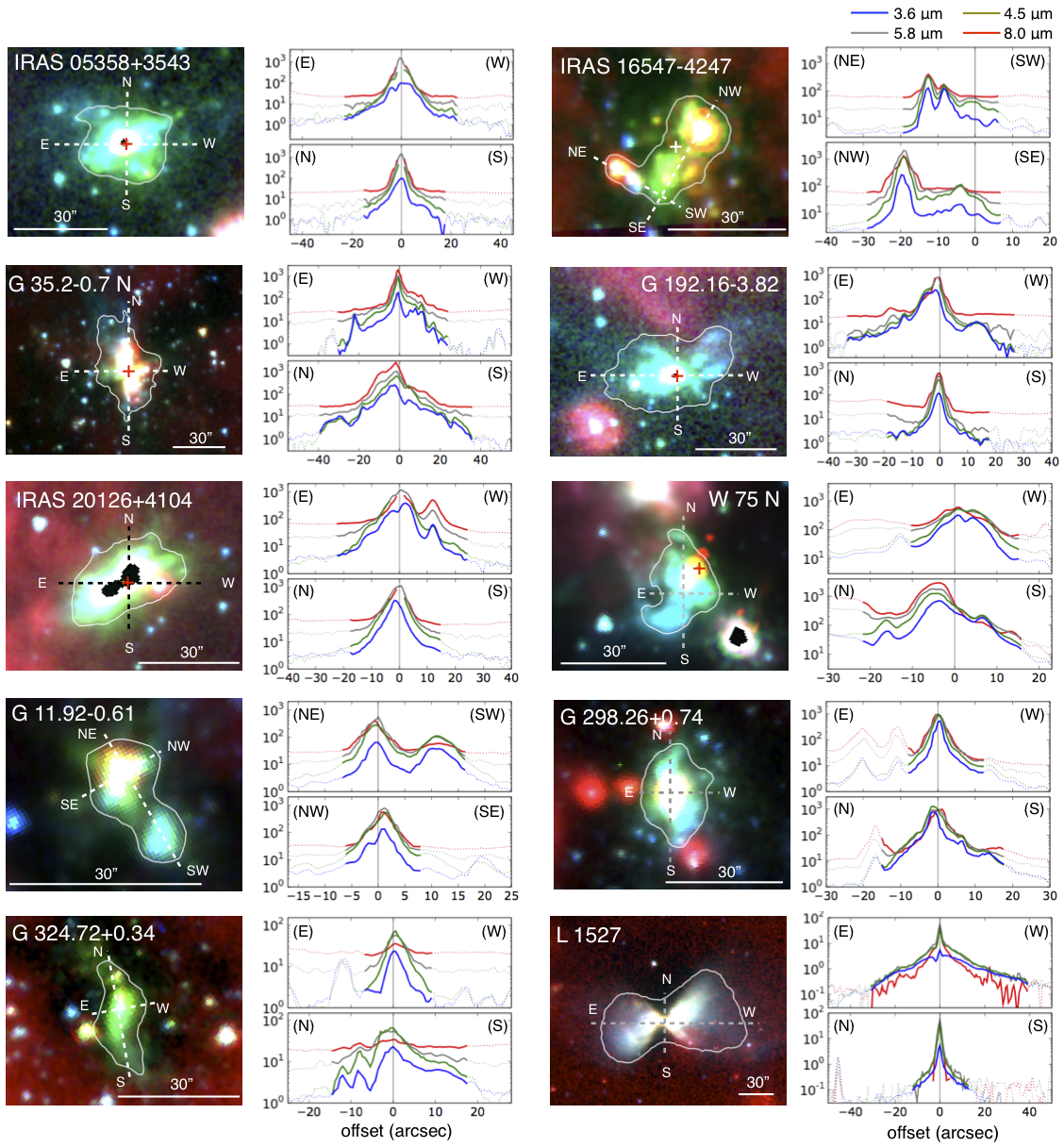
Figure 1: Three-color images (blue, green, and red for 3.6, 4.5 and 8.0 µm, respectively) and one dimensional intensity distributions (blue, green, gray and red for 3.6, 4.5, 5.8 and 8.0 µm, respectively) for individual objects. In all the three colors north is up and east is right. For the these images the color contrasts were set with the upper and lower limits based on the specified percentage of the flux in the entire image (see text). The saturated regions near these positions are masked in black. The small cross in each three-color-image shows the position of the protostar (HPMOs, HC/UC H IIs) measured using millimeter interferometry (see Table 2 for references). The white curve in the three-color image indicates the region where we measured the flux ratios and colors. The positions where we extract the one dimensional intensity profiles are marked using dotted lines. In the one-dimensional profiles, the flux outside these positions is indicated using dotted curves. In these plots the flux is shown in logarithmic scale in MJy str^-1.

The Spitzer IRAC data in all four bands (3.6, 4.5, 5.8, and 8.0 µm) were obtained from the Spitzer archive. We use the pipeline reduced post-BCD (Basic Calibration Data) images provided by the archive. The mean FWHMs of the point response functions (PRFs) are 1”.66, 1”.72, 1”.88 and 1”.98, respectively. Figure 1 shows the conventional three color images: blue, green, red for 3.6, 4.5, and 8.0 µm, respectively, as well as one-dimensional cut-outs of the intensity distributions in all four bands. All the objects are associated with Green Fuzzy emission, and the one-dimensional profiles show that these have a similar shape at 3.6, 4.5, and 5.8 µm.

Our contrast adjustment for the three colors in Figure 1 was made by setting the upper and lower limits based on the specified percentage (95, 96, 97, 98, 99 or 99.5 %, depending on the objects) of the flux distribution in the larger areas. As a result, stars can appear blue due to the fact that the flux is larger at shorter wavelengths; PAH emission can appear red due to excessive emission at 8.0 µm; the remaining extended emission can appear green due to relatively low fluxes of stars and PAH at this wavelength. While other authors (Noriega-Crespo et al., 2004; Marston et al., 2004; Rathborne et al., 2005; Smith et al., 2006; Araya et al., 2007; Kumar and Grave, 2007; Shepherd et al., 2007; Tobin et al., 2007, 2008; Qiu et al., 2008; Teixeira et al., 2008; Cyganowski et al., 2008, 2009, 2011; Chambers et al., 2009; Morales et al., 2009; Zhang and Wang, 2009; Simpson et al., 2009; Varricatt, 2011) do not clearly state their color adjustments, we assume that most, if not all, of them made it in a more or less similar manner.

Despite the “green” color in the three color image, none of the sources clearly show excess emission at 4.5 µm in the one-dimensional cut-outs in Figure 1. Indeed, Chambers et al. (2009), who coined the term Green Fuzzies, define a quantitative criteria for their detection as a 4.5 µm to 3.6 µm  ratio of $\geq$ 1.8 and a 5.8 µm to 4.5 µm  ratio of $\leq$ 2.5. Plotting this criteria, one can easily find that those with a marginal deficit at 4.5 µm can also be categorized as Green Fuzzies. Throughout, the green color in three-color images may not always imply the presence of the 4.5-µm emission enhanced over the other IRAC bands as stated in the literature (e.g., Rathborne et al., 2005; Araya et al., 2007; De Buizer and Vacca, 2010).

Figure 1 also indicates the regions in each object where we apply our analysis with flux ratio maps and the pixel by pixel color-color diagrams. The criterion is described in Section 3. Throughout the paper we focus the analysis on the brightest regions (contrast ratio to the brightest pixels to be 1/10–1/100) where we expect high signal-to-noise. This means that our analysis misses the faint outer regions discussed in previous literature in the W 75 N (Qiu et al., 2008) and G 11.92–0.61 regions (Cyganowski et al., 2008, 2009, 2011).

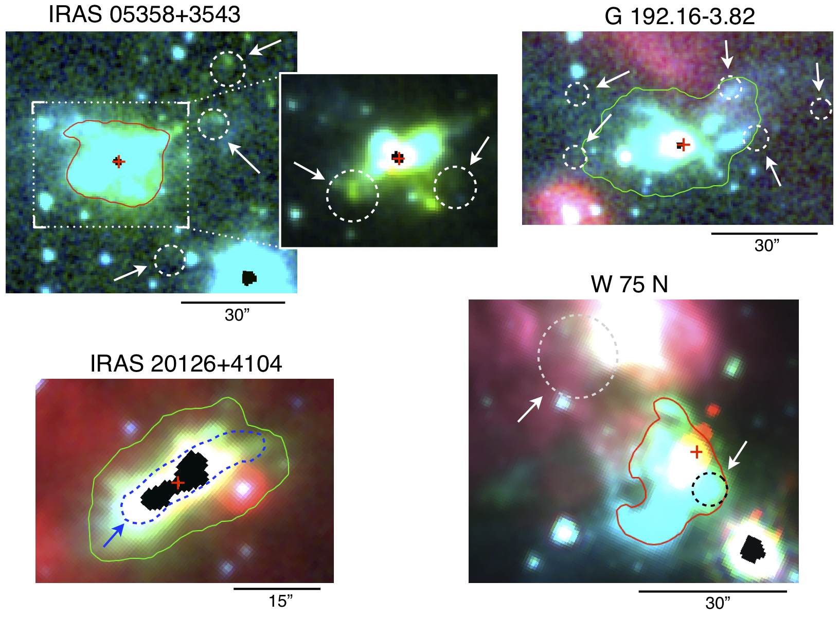
Figure 2: Three-color images for IRAS 05358+3543, G 192.16–3.82, IRAS 20126+4104, and W 75 N with different contrasts from Figure 1. In all the three colors north is up and east is right. Dashed circles, curves and rectangles with arrow are the positions where the presence of H₂ 2.12 µm emission was reported in the literature (Varricatt et al. 2010 for IRAS 05358+3543, G 192.16–3.82, and IRAS 20126+4104; Davis et al. 1998 for W 75 N). The regions where we measured the flux ratios and colors are also indicated using red or green curves.

Imaging observations of H₂ at 2.12 µm  have been made near these bright regions for all the nearby high-mass protostar sample. These are:- IRAS 05358+3543 (Varricatt et al., 2010), IRAS 16547–4247 (Brooks et al., 2003), G 35.2–0.7 N (Froebrich et al., 2011; Lee et al., 2012), G 192.16–3.82 (Indebetouw et al., 2003; Varricatt et al., 2010), IRAS 20126+4104 (Shepherd et al., 2000; Varricatt et al., 2010), and W 75 N (Davis et al., 1998; Shepherd et al., 2003). The H₂ 2.12 µm emission in IRAS 05358+3543, G 192.16–3.82, and W 75 N are identified as knots, while that in IRAS 20126+4104 exhibits a collimated jet. These contrast to the fuzzy morphology of the green emission in Figure 1. Figure 2 shows the locations of the H₂ emission in the three-color images. At these positions only faint 4.5-µm emission components are seen at some of these positions. The H₂ 2.12 µm emission in IRAS 16547–4247 and G 35.2–0.7 N show more complicated structures in shocked gas (Brooks et al. 2003; Froebrich et al. 2011, Lee et al. 2012). These have a significantly larger spatial extension (by a factor of 2–3) than the bright IRAC emission shown in Figure 1, and most of the flux is distributed outside the region indicated.

Most of the above literature also provide the continuum images at $\sim$2 µm, either $K(2.2\micron)$, $K$’ (2.12 µm), $K_{s}$ (2.15 µm) or 2.14 µm. Their distributions in IRAS 05358+3543, G 35.2–0.7 N, G 192.16–3.82, IRAS 20126+4104, and W 75 N are remarkably different from H₂ 2.12 µm, but to some extent similar to the IRAC emission in Figure 1. In particular, a bipolar structure is observed in G 35.2–0.7 N and G 192.16–3.82 in both IRAC and the continuum at 2-µm (see Froebrich et al., 2011; Indebetouw et al., 2003; Varricatt et al., 2010). In the west of G 192.16–3.82 both IRAC emission and 2-µm continuum show a horn-like structure at similar angular scales. In W 75 N, both IRAC emission and 2-µm  continuum are extended to the south-east side of the protostar, in contrast to the orientation of the molecular outflow (Shepherd et al., 2003) and the distribution of H₂ emission in different directions (Davis et al., 1998; Shepherd et al., 2003). The detection of the 2-$\micron$ continuum at these positions indicates that the different distribution seen in the bright parts of Green Fuzzy emission and H₂ 2.12 µm may not be attributable to extinction (Lee et al., 2012).

Molecular outflows have been observed in most of our nearby high-mass protostar sample. G 35.2–0.7 N and G 192.16–3.82 are associated with molecular outflows with similar morphology to the direction of elongation in the Green Fuzzy emission (Gibb et al., 2003; Shepherd et al., 1998), but the position angles between the Green Fuzzies and molecular outflows are different by $\sim 30^{\circ}$. In IRAS 05358+3543 and W 75 N, the distribution of Green Fuzzy emission is remarkably different from the molecular outflows observed at millimeter wavelengths by Beuther et al. (2002); Davis et al. (1998); Shepherd et al. (2003) (see also Qiu et al., 2008). For IRAS 16547–4247, Brooks et al. (2003) shows the presence of extended shocked H₂ emission to the north and south of the protostar. This contrasts to the distribution of Green Fuzzy emission in Figure 1. In IRAS 20126+4104 Cesaroni et al. (1999) shows the presence of a molecular outflow in the millimeter HCO⁺ and SiO emission with the same orientation as the Green Fuzzy emission in Figure 1, but with a slightly smaller angular scale. This object is also associated with a more extended outflow in the millimeter CO emission with a remarkably different orientation (Shepherd et al., 2000).

3 Flux Ratio Maps and Color-Color Diagrams

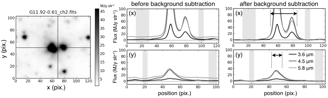
Figure 3: Examples of background subtraction. ($left$) the $I_{4.5\micron}$ image of the objects after convolution. The coordinates are shown in pixels (1 pixel correspond to 0”.6). The crosshair in the image shows the positions where we measured the one-dimensional flux distribution for background subtraction. ($middle$) one-dimensional intensity profiles at 3.6, 4.5 and 5.8 µm  before subtracting the background. Gray squares show the range where we measured the background level and its standard deviation after background subtraction (i.e., the uncertainty of the flux measurement for the flux ratio maps and color-color diagrams). ($right$) same as the middle but after background subtraction. The arrows and dashed lines show the spatial ranges for $>$$15\sigma$ ($>$18.7 MJy str^-1) for the 4.5-µm emission. This corresponds to the region we selected for the color-color diagrams (see text for details).

In most of the regions the emission at 8.0 µm  is severely contaminated by bright diffuse extended emission not directly associated with the protostar. Therefore, we will use the data for 3.6, 4.5, and 5.8 µm, excluding 8.0 µm. To produce accurate flux ratio maps and color-color diagrams, the individual images need to be matched in resolution and carefully background subtracted. We first convolve each image with the appropriate PRFs to try to cancel out the effect of different PRFs at 5.8 µm from 3.6 and 4.5 µm (note that the PRFs at 3.6 and 4.5 µm  are almost identical — see IRAC Data Handbook 3.0). The 3.6 and 4.5 µm images are convolved with the PRF at 5.8 µm, and the 5.8 µm images with the PRF at 3.6 µm. This yields an effective angular resolution of $\sim$3”. We then subtract the diffuse background emission by measuring it in the $x$- and $y$-directions, and fitting it using a linear function. Figure 3 shows how this process works for one of our sample. This fitting process simultaneously allows us to measure the uncertainty of flux, which is dominated by non-uniform distribution of diffuse emission. These are tabulated in Table 2.

To investigate the origin of the Green Fuzzy emission, we use pixel by pixel color-color diagrams with [3.6]-[4.5] and [3.6]-[5.8]. As described in Section 2, we focus the analysis on the brightest regions where we expect the high signal-to-noise to clearly show the tendencies in color-color diagrams described later. The criterion for selection is summarized in Table 2. The selection is made based on the 4.5-µm flux: $>$15-$\sigma$ for most of the objects. For W 75 N and G 298.26+0.74 a larger limit is applied to exclude the emission associated with other object(s) nearby. For IRAS 20126+4104 we apply an additional flux limit ($>$5-$\sigma$) for 5.8-µm. This allows us to remove artifacts in the color-color diagrams that are due to a high uncertainty in the background subtraction at this wavelength for this object. For L 1527 a flux limit of $>$25-$\sigma$ is applied to clearly show the linear correlation between [3.6]-[4.5] and [3.6]-[5.8] described later. In all the objects we rebin the data onto a 3” grid, i.e., the same angular scale as the resolution after convolution.

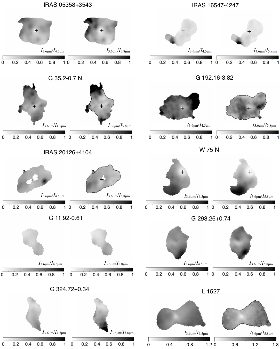
Figure 4: The $I_{3.6\micron}/I_{4.5\micron}$ and $I_{3.6\micron}/I_{5.8\micron}$ maps for individual objects. In all the three colors north is up and east is right. The region is selected based on the criterion in Table 2. The range of grayscale for the $I_{3.6\micron}/I_{4.5\micron}$ and $I_{3.6\micron}/I_{5.8\micron}$ maps is 0–1 for all figures but L 1527 (0–1.2 and 0–1.8 for this object). The cross shows the position of the protostar (HPMOs, HC/UC H IIs) measured using millimeter interferometry (see Table 2 for references). The saturated regions near these positions are masked in white. Black curves are drawn in the $I_{3.6\micron}/I_{5.8\micron}$ maps for G 35.2-0.7 N, G 192.16-3.82, IRAS 2016+4104 and L 1527, and these are the regions selected for color-color diagrams excluding stars near the boundary. For the other objects the entire region shown in the figure is used for color-color diagrams.

Figure 4 shows the 3.6/4.5- and 3.6/5.8-µm  flux ratios maps in the regions described above. This figure shows that the the distributions of the 3.6/4.5- and 3.6/5.8-µm  flux ratios are similar for each object except G 192.16–3.82. IRAS 20126+4104, G 35.2-0.7N, G192.16-3.82, and L 1527 are associated with stars near the boundary. These appear blue in three-color images in Figure 1, and exhibit high 3.6/4.5- and 3.6/5.8-µm  flux ratios ratios in the flux ratio maps in Figure 4. The color-color diagrams for these objects are made excluding these stars. The regions after this removal are indicated in Figure 4 as well as Figure 1. In IRAS 20126+4104, the 3.6/4.5-µm  flux ratio map shows another point source with high flux ratios in the west of the region. This source is absent or marginal in the 3.6/5.8-µm map. The inferred color of this source and the rest of the region is discussed later.

In Figure 4 we also plot the positions of the protostar (HPMO, HC/UC H II) measured using millimeter interferometry. Although the position is in the mask of low signal-to-noise or a saturated region for a few objects, this approximately matches the region with the lowest 3.6/4.5- and 3.6/5.8-µm flux ratios. Similarly, these flux ratios are the lowest at the center of L 1527 where the protostar is located (Tobin et al., 2008).

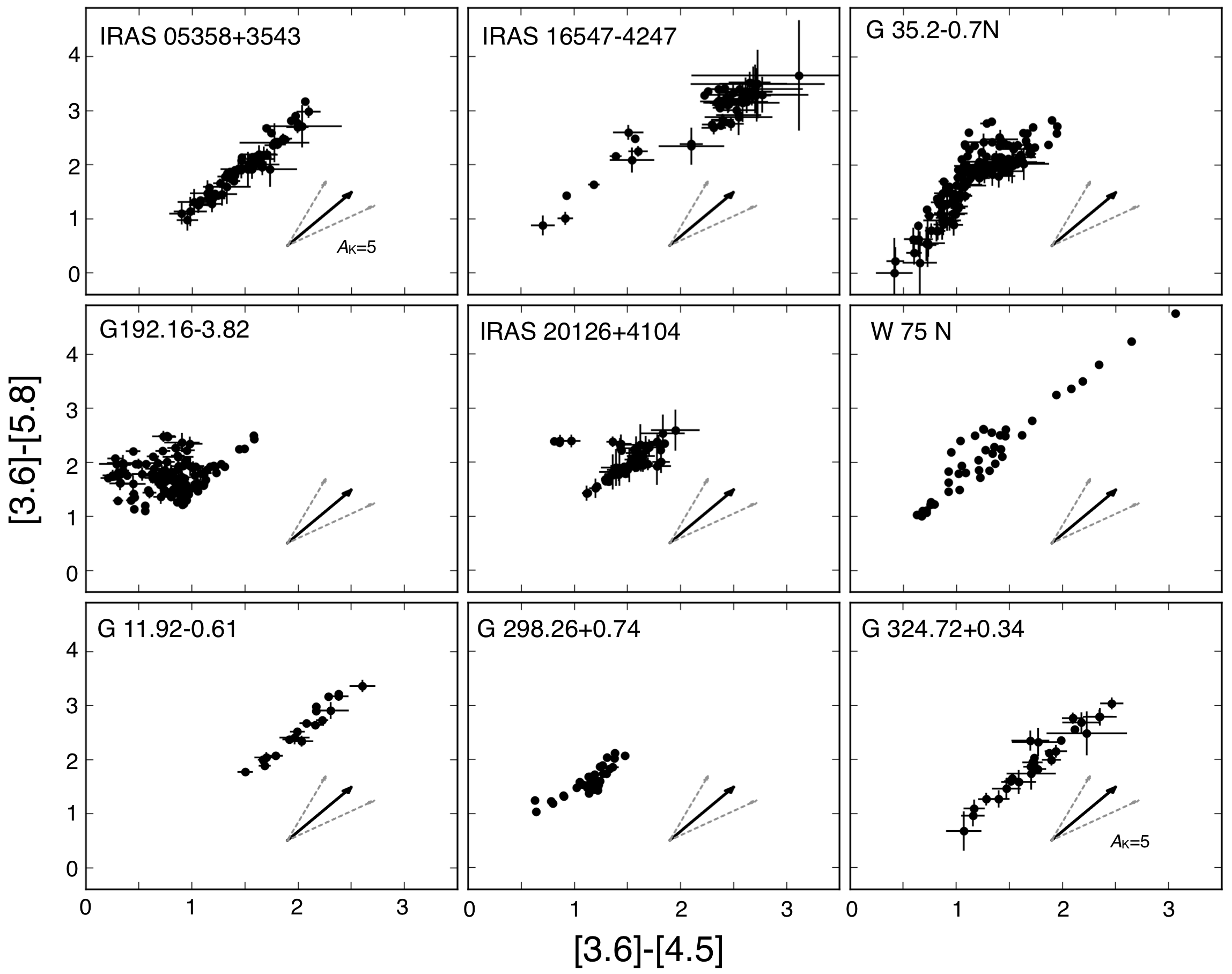
Figure 5: The [3.6]-[4.5] versus [3.6]-[5.8] colors measured in “Green Fuzzies” in ten high-mass star forming regions. The error bars are shown only for those larger than the size of the dots. The solid arrows show the extinction vector based on the measurements of molecular clouds ([3.6]-[4.5] and [3.6]-[5.8] of 0.09$\pm$0.03 and 0.18$\pm$0.03, respectively, at $A_{K}\geq 2$; Chapman et al. 2009). Gray arrows show the extinction vectors at $\pm$1-$\sigma$.

Figure 5 shows the colors measured in the 3$\times$3 arcsec image bins for Green Fuzzy emission in each high-mass star forming region. All the objects but IRAS 20126+4104 and G 192.16-3.82 show a fairly strong correlation between the [3.6]-[4.5] and [3.6]-[5.8] colors along the direction of the extinction vector. Their values vary between objects in the ranges of [3.6]-[4.5] and [3.6]-[5.8] of 0.4–3 and 0.1–4.7, respectively. A similar trend is also observed in most of pixels selected in Green Fuzzy emission associated with IRAS 20126+4104. In addition to the component in which the [3.6]-[4.5] and [3.6]-[5.8] colors show a linear correlation, this object is associated with several pixels for which [3.6]-[5.8] is constant (2.2–2.4) over [3.6]-[4.5] =0.8–1.5. Some pixels in G 192.16-3.82 also show a linear correlation like that described above, however, this object is also associated with a number of pixels with larger [3.6]-[4.5] and [3.6]-[5.8] colors, ranging between 0.2–1.7 and 1.0–2.4 for [3.6]-[4.5] and [3.6]-[5.8], respectively.

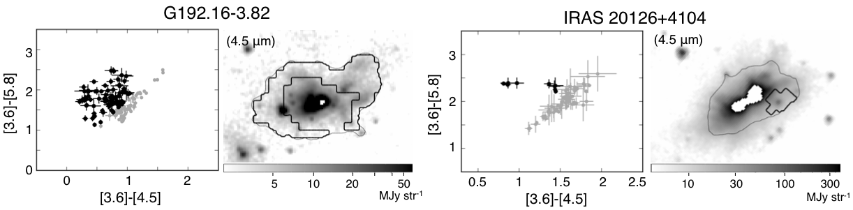
Figure 6: Emission deviating from the linear color correlation in the G 192.16–3.82 and IRAS 20126+4104 regions, and their spatial distributions in the 4.5-µm image. The black and gray dots in the color-color diagrams show the deviating and remaining components of the [3.6]-[4.5] and [3.6]-[5.8] colors. In the 4.5-µm image the former is shown with thick curves, while the entire region used for the color-color diagrams are shown with thin curves.

Figure 6 shows the locations of the regions which have a [3.6]-[5.8] excess from the linear correlation in G 192.16–3.82, and where the [3.6]-[5.8] color has a constant value in IRAS 20126+4104. In G 192.16–3.82 the [3.6]-[5.8] excess is located in the outer regions where the 4.5-µm flux is relatively faint. In IRAS 20126+4104 the emission with a constant [3.6]-[5.8] is located around a point source to the west of the protostar. The latter is also clearly seen in the 3.6/4.5-µm flux ratio map in Figure 4. These areas are responsible for a small fraction of the 4.5-µm flux as compared with that of the entire area shown with dashed curves: these are 22 % and 6 % for G 192.16–3.82 and IRAS 20126+4104, respectively.

Some authors mention the possibility that such “green emission” is due to CO ro-vibrational transitions at 4.5-5 µm (see e.g., Shepherd et al., 2007; Cyganowski et al., 2008, 2009; Chambers et al., 2009, ; see also Takami et al. 2010 and reference therein). However, our results do not show clear evidence for such emission components, which should only appear in the 4.5-µm band. If the Green Fuzzy emission in these objects is associated with shocked emission as discussed by some authors (see Section 1), the absence of CO emission contrasts to the shocks associated with low-mass protostars, which also show green colors in three-color images (e.g., Noriega-Crespo et al., 2004; Tobin et al., 2007; Teixeira et al., 2008; Zhang and Wang, 2009). In the latter a 4.5-µm excess, presumably due to CO emission, is observed at some positions in most of the objects in Takami et al. (2010, 2011). In the next two sections we discuss the emission mechanism of Green Fuzzy emission associated with high-mass protostars and their candidates.

4 Comparisons with Other Objects and Models in Color-Color Diagrams

In the following subsections we compare these colors with scattered continuum (Section 4.1), molecular shocks associated with low-mass protostars and modeled thermal H₂ emission (Section 4.2), and PAH and fluorescent H₂ emission (Section 4.3).

4.1 Scattered continuum

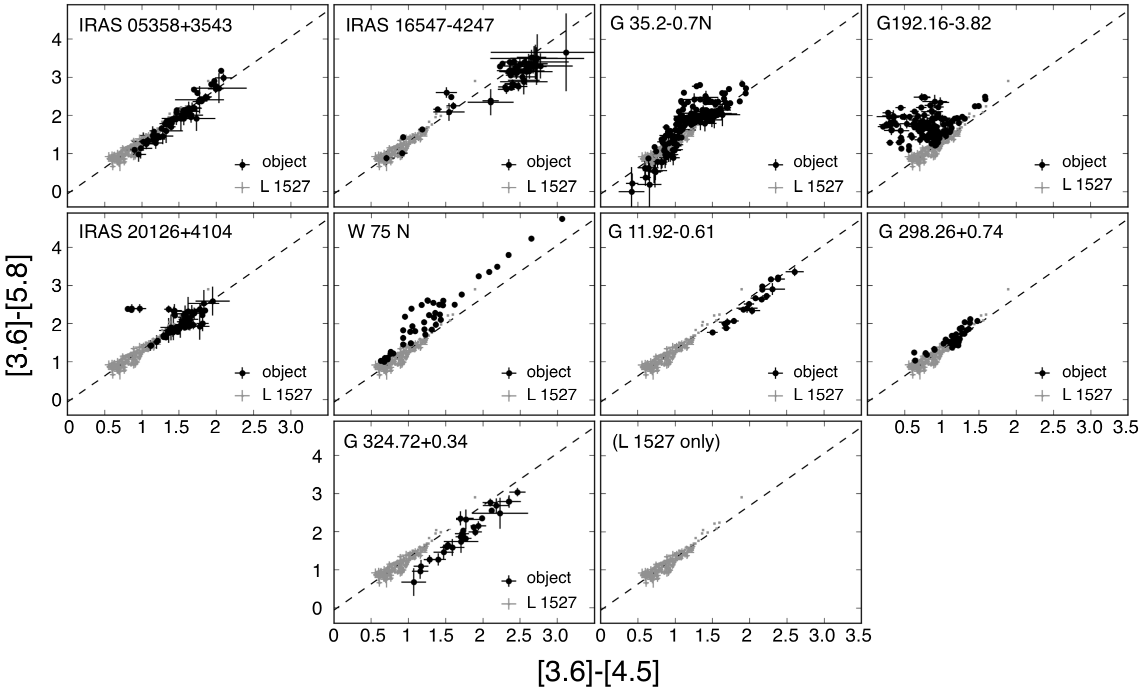
Figure 7: Same as Figure 5 but with colors measured in the scattered continuum in the L 1527 outflow. The dashed line shows the regression line for the results of L 1527 ([3.6]-[5.8]=[3.6]-[4.5]$\times$1.374–0.067).

Figure 7 shows the same color-color diagrams as Figure 5 but we include the points for scattered continuum from the L 1527 protostellar outflow in each diagram. The correlation of [3.6]-[4.5] and [3.5]-[5.8] colors observed in most of the high-mass star forming regions is remarkably similar to that of L 1527. The regression line for L 1527 fits the observed colors in IRAS 05358+3543, IRAS 16547–4247, G 298.26+0.74, and most of the colors measured in IRAS 20126+4104 as well. The figure shows a slightly larger [3.6]-[5.8] color (up to 0.6) in W 75 N and a slightly smaller [3.6]-[5.8] color (by 0.3–0.7) in G 11.92–0.61 and G 324.72+0.34 compared with the regression line. G 35.2–0.7 N and W 75 N show a [3.6]-[5.8] excess at [3.6]-[4.5]=1.0–1.5.

If the Green Fuzzy emission in our sample of high-mass star forming regions is due to scattered continuum, the observed colors should be a function of: (1) the intrinsic color of the central star(+disk); (2) the color change due to scattering; and (3) extinction. To investigate the first two issues, we have made simplified calculations with existing star-disk models and dust models. The modeled colors for star-disk systems were obtained from Robitaille et al. (2006), based on radiative transfer calculations for protostellar environments with the protostar, disk, envelope and outflow cavities by Whitney et al. (2003b). Robitaille et al. (2006) present a grid of infrared spectral energy distributions (SEDs) for 200,000 cases, with a variety of stellar and disk parameters, at ten viewing angles for each model. To derive the infrared flux from the disk, these authors include “active viscous heating based on the standard accretion disk model by Shakura and Sunyaev (1973), and “passive heating by stellar radiation. They also adopt the disk geometry of Shakura and Sunyaev (1973).

To derive the intrinsic color of the star-disk systems (i.e., “1” described above), we select all the modeled results with $A_{V}<5$ (corresponding to $E_{3.6\micron-4.5\micron}<0.07$ and $E_{3.6\micron-5.8\micron}<0.12$ for the adopted grain model). This criterion is applied due to the fact that the Robitaille et al. (2006) models apparently include dust in the envelope and outflow cavity so that we cannot derive the values without extinction. The above criterion allows us to include a large number of samples with a variety of disk masses and accretion rate with small errors in color due to extinction. We also select all the results with a stellar mass larger than 8 $M_{\odot}$. As a result, a total of 17,580 SEDs are selected from the grid, with a range of stellar mass $M_{*}$=8–50 $M_{\odot}$, stellar effective temperature $T\sim 4\times 10^{3}-5\times 10^{4}$ K, disk mass 0–3 $M_{\odot}$, and accretion rate $M\sim 10^{-14}-10^{-3}~{}M_{\odot}$ yr^-1 if the system hosts a disk. In addition to the modeled colors of Robitaille et al. (2006), we calculate the color for blackbodies with a single temperature of $T$=500, 1000 and 4000 K.

The color change via single scattering is derived from Robitaille et al. (2006), with the grain models based on the optical constants and size distribution by Laor and Draine (1993) and Kim et al. (1994), respectively. We consider the following two cases for scattering: (1) scattering in optically thin regions, i.e., where the color change via scattering is determined by the scattering cross section at each wavelength; and (2) scattering for optically thick and geometrically thin cavity walls, which may be realistic for outflow cavities associated with low-mass protostars (e.g., Whitney et al., 2003a; Tobin et al., 2008). For the latter, the efficiency of the scattering should be approximately determined by the scattering albedo, assuming that the effects of internal extinction and multiple scattering are negligible. For the color change due to extinction, the extinction vector based on Chapman et al. (2009) has a large uncertainty as shown in Figure 5. Here we assume that the linear correlation observed in L 1527 is due to different extinction at different positions, and extract the values from the regression line.

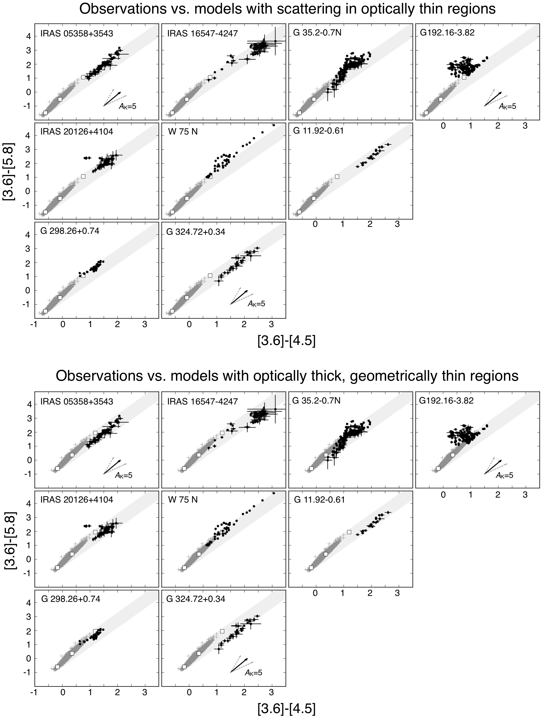
Figure 8: Same as Figure 5 but with scattering for models of the optically thin cases (upper) and optically thick but geometrically thin cases (lower). The colors for the objects are shown with black dots, with error bars if they are larger than the dots. Gray crosses show the colors for star-disk systems (Robitallile et al. 2006) with scattering. Open squares show the colors for a blackbody ($T$=4000, 1000 and 500 K from the lower-left to the upper-right) with scattering. The gray areas show the modeled colors, adding arbitrary extinction, assuming that the linear correlation observed in L 1527 is due to different extinction between positions.

Figure 8 shows the modeled colors of the star-disk systems with scattering together with the observed colors. This figure shows that colors of these objects approximately lie within the extinction track of either the optically thin or thick results. In this case, the linear correlation of the [3.6]-[4.5] and [3.6]-[5.8] colors in each object is attributed to different extinctions at different positions. The different objects show different colors not only in the direction of the extinction vector, but also across it. The latter is consistent with the idea that the intrinsic color of the star(+disk) systems differs between objects. In IRAS 05358+3543, G 11.92–0.61, and G 324.72+0.34, the intrinsic flux of the central source is dominated by a star with a relatively high color temperature ($T>$1000 K). In W 75 N and G 298.26+0.76, the central source is redder, i.e., its flux is dominated by a protostar with a relatively low color temperature ($T<$1000 K). Figure 8 also shows that the two different scattering models yield similar results for the color of the embedded central source.

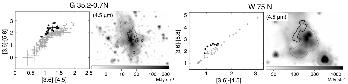
Figure 9: Same as Figure 6 but for G 35.2–0.7 N and W 75 N regions.

In G 35.2–0.7 and W 75 N the distribution of the correlation is broader, the [3.6]-[5.8] color partially exceeding those expected for the models at [3.6]-[4.5] $\sim$1. Figure 9 shows their distribution in the 4.5-µm map. These areas are responsible for 34 % and 9 % of the 4.5-µm flux integrated over the entire area shown in dashed curves in G 35.2–0.7 and W 75 N, respectively.

4.2 Shocks in low-mass protostellar jets, thermal H₂ emission

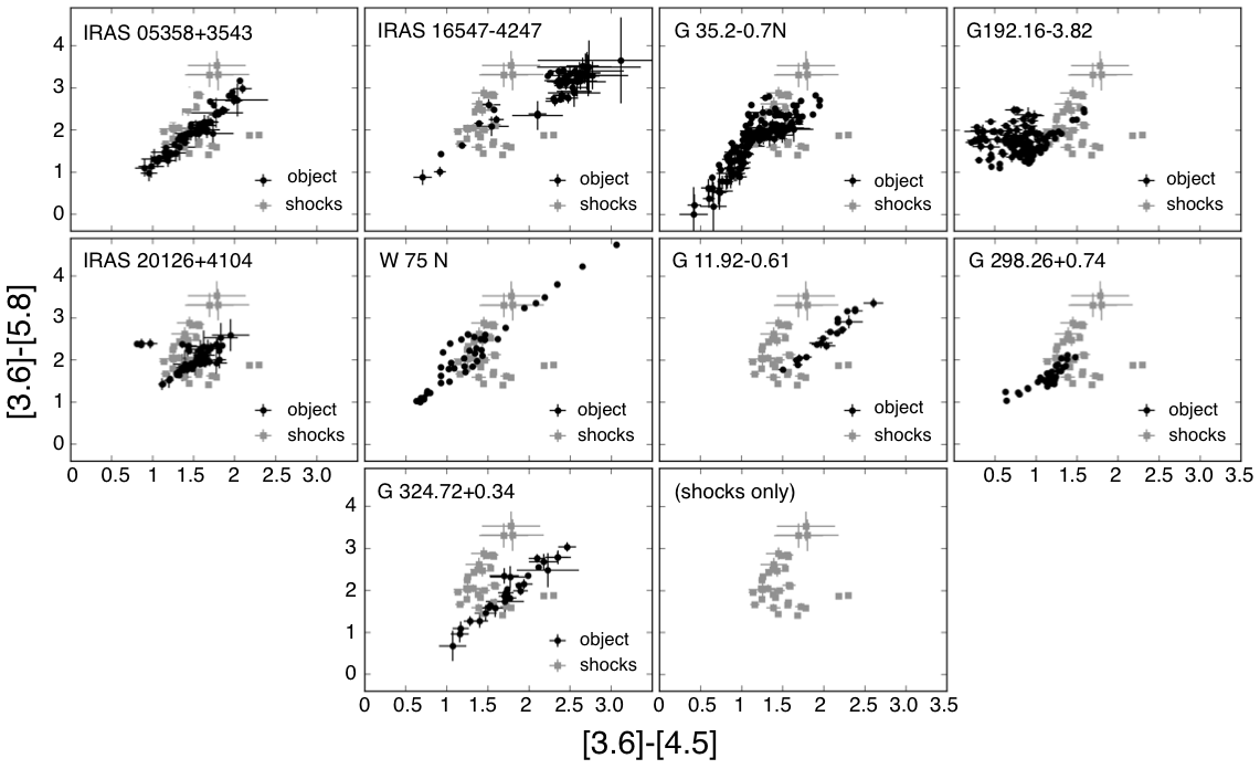
Figure 10: Same as Figure 5 but with those observed in shocks associated with low-mass protostars. The error bars are shown only if they are larger than the dots.

Figure 10 shows the same color-color diagrams as Figures 5 and 7 but with the colors observed in six low-mass protostellar jets analyzed by Takami et al. (2010). They showed that while some of them are explained by thermal H₂ emission (a combination of rotational and ro-vibrational transitions), others requires additional emission at 4.5 µm, presumably due to the vibrationally excited CO emission. In Figure 10, the colors are distributed along an arc with [3.6]-[4.5] and [3.6]-[5.8] of 1.1–2.3 and 1.4–3.5, respectively, located at both sides of the linear color correlation observed in most of the objects. While the observed correlations between [3.6]-[4.5] and [3.6]-[5.8] are totally different between Green Fuzzy emission and shocks associated with low-mass protostars, their colors match in some color ranges in most of the objects. The range of such colors are [3.6]-[4.5] = 1.2–1.6 and [3.6]-[5.8] = 1.5–2.5 for IRAS 05358+3543, G 192.16–3.82, IRAS 20126+4104, W 75 N and G298.26+0.74. This color range is slightly larger in G 35.2–0.7 N ([3.6]-[4.5] = 1.1–1.6 and [3.6]-[5.8] = 1.6–2.8), while IRAS 20126+4104 has an additional overlap at [3.6]-[4.5] = 1.3 and [3.6]-[5.8] = 2.4.

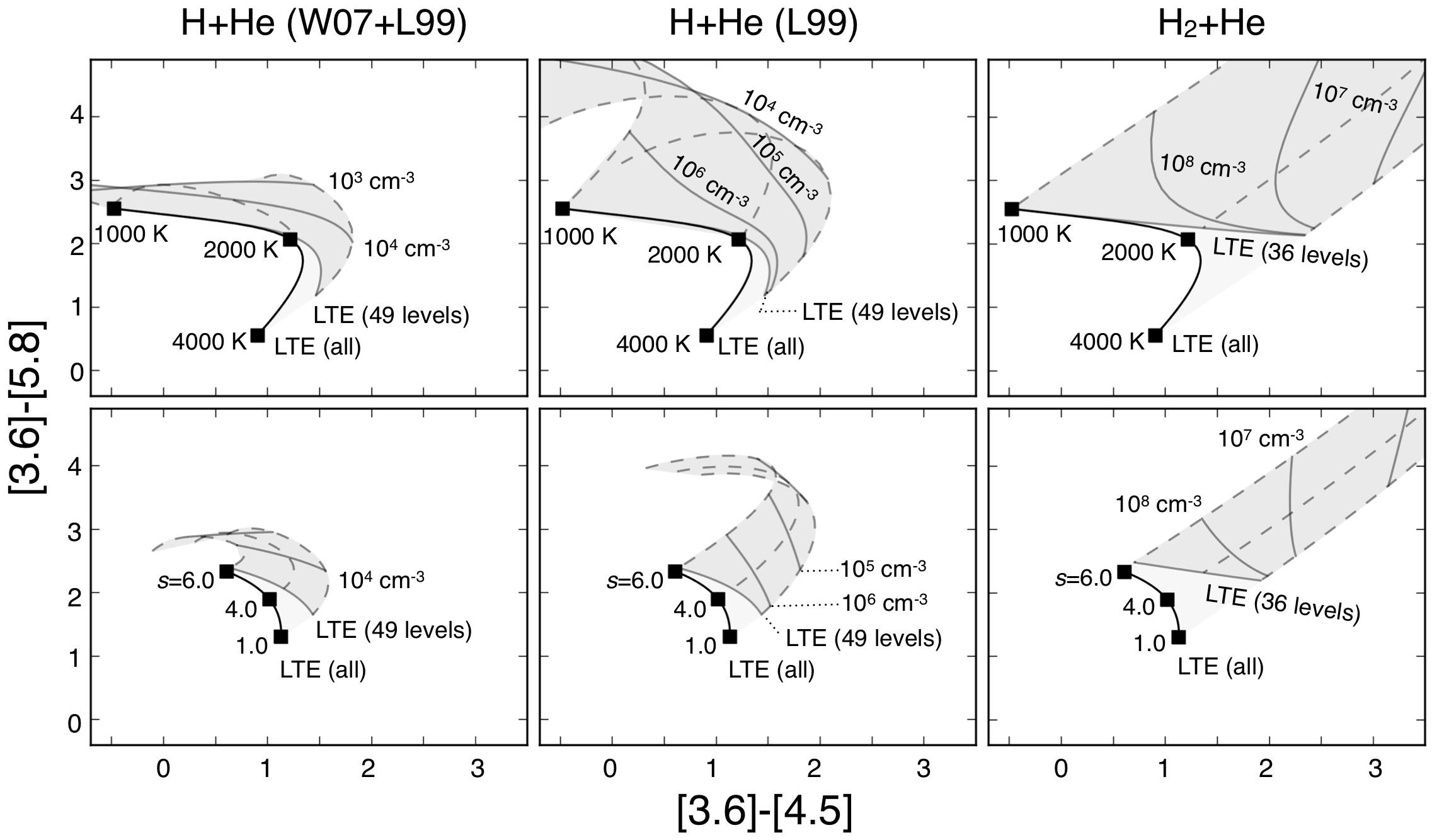
Figure 11: Colors of thermal H₂ emission for LTE with all the transitions (solid curves) and non-LTE with 36/49 levels (dark gray area). The upper and lower figures are for isothermal cases and temperature structures determined by a power-law cooling function ($\Lambda\propto T^{s}$), respectively. The left plots are for collisions with H+He based on the collisional rate coefficients of H and He by Wrathmall et al. (2007) and Le Boutlot et al. (1999), respectively; middle are the same but the coefficients of H and He both by Le Boutlot et al. (1999); right are the same as middle but for collisions with H₂ and He. Gray solid and dashed curves show colors with the same density and temperature (or temperature structure determined by the power-law index), respectively. The light gray areas show the gap between LTE calculations for all and those with limited numbers of the transitions (see text).

Figure 11 shows the colors for thermal H₂, i.e., the primary source of H₂ emission in shocks, based on calculations by Takami et al. (2010). As in Takami et al. (2010) the models are made for iso-thermal cases and shock slabs with a power-law cooling function ($\Lambda\propto T^{-\alpha}$). The latter has been used to explain shocked H₂ emission observed both from the ground (e.g., Brand et al., 1988; Gredel, 1994; Everett et al., 1995; Richter et al., 1995; Takami et al., 2006) and in space (Neufeld and Yuan, 2008; Neufeld et al., 2009; Takami et al., 2010). For calculations of non-local-thermal-equilibrium (non-LTE) cases thermal collisions are included for two cases, H+He and H₂+He, corresponding to gas with relatively high ($\gg 0.002-0.02$) and low ($\ll 0.002-0.02$) dissociation rates (Takami et al., 2010). We adopt $A$-coeffcients provided by Wolniewicz et al. (1998), and collisional rate coefficients for H₂ and He by Le Bourlot et al. (1999). For collisional rate coefficients of H, we adopt Wrathmall et al. (2007) and Le Bourlot et al. (1999), and show the results separately. According to Wrathmall et al. (2007), they provide rate coefficients with a better accuracy than Le Bourlot et al. (1999) due to improved representation of the vibration eigen functions. In contrast, the coefficients provided by Le Bourlot et al. (1999) can explain the observed IRAC colors better in Takami et al. (2010).

The energy levels we include for calculations are 245 ($E_{u}/k=0-43000$ K) for LTE based on all the levels included in Draine and Bertoldi (1996); the lowest 49 energy levels (46 lines in the IRAC four bands, $E/k$ up to $2\times 10^{4}$ K) for non-LTE H₂ with H+He collisions; and the lowest 36 energy levels (32 lines in the IRAC four bands, $E/k$ up to $1.69\times 10^{4}$ K) for non-LTE H₂ with H₂+He collisions. The number of transitions included for non-LTE calculations is limited by the availability of collisional rate coefficients. The level populations of ortho- and para-H₂ are calculated separately, and those fluxes are combined assuming an ortho/para ratio of 3. The upper limit of temperature is set at 4000 K, approximately corresponding to the dissociation temperature of H₂ molecules (e.g., Lepp and McCray, 1983). We set the lowest temperature of 30 K for numerical integration of the temperature slabs for power-law cooling. Since the emission in IRAC bands should originate from gas at much higher temperature ($\gtrsim$1000 K Takami et al., 2010), this limit does not affect the colors we show in Figure 11. For all the above cases the measured spectral response functions are used to obtain the IRAC fluxes.

Due to the limited number of transitions included, the accuracy of non-LTE calculations are low for the IRAC 3.6-µm band at the highest temperatures. The gaps between such calculations and those with 245 levels are also shown in Figure 11 for the LTE regimes. The non-LTE gas of our calculations does not show smaller [3.6]-[4.5] and [3.6]-[5.8] colors than LTE, since the 3.6-µm emission requires a higher density for thermalization than the emission in the other IRAC bands (Takami et al., 2010).

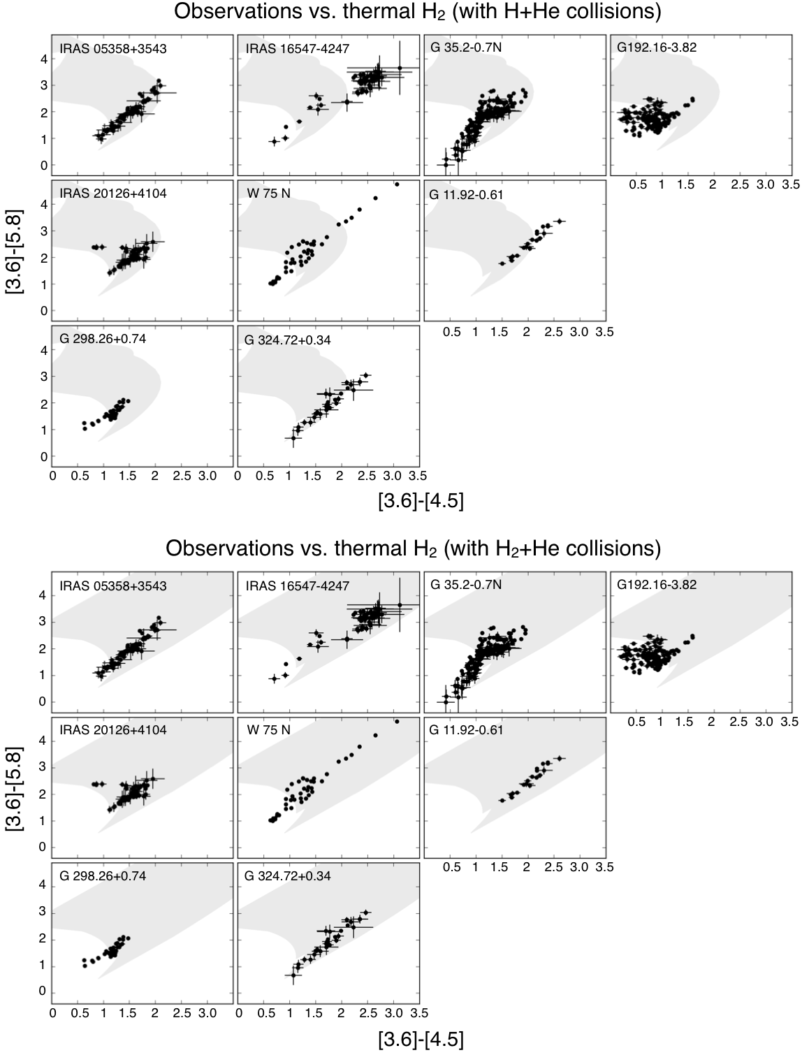
Figure 12: Same as Figure 5 but with the possible coverage for thermal H₂ emission (gray area) shown in Figure 11.

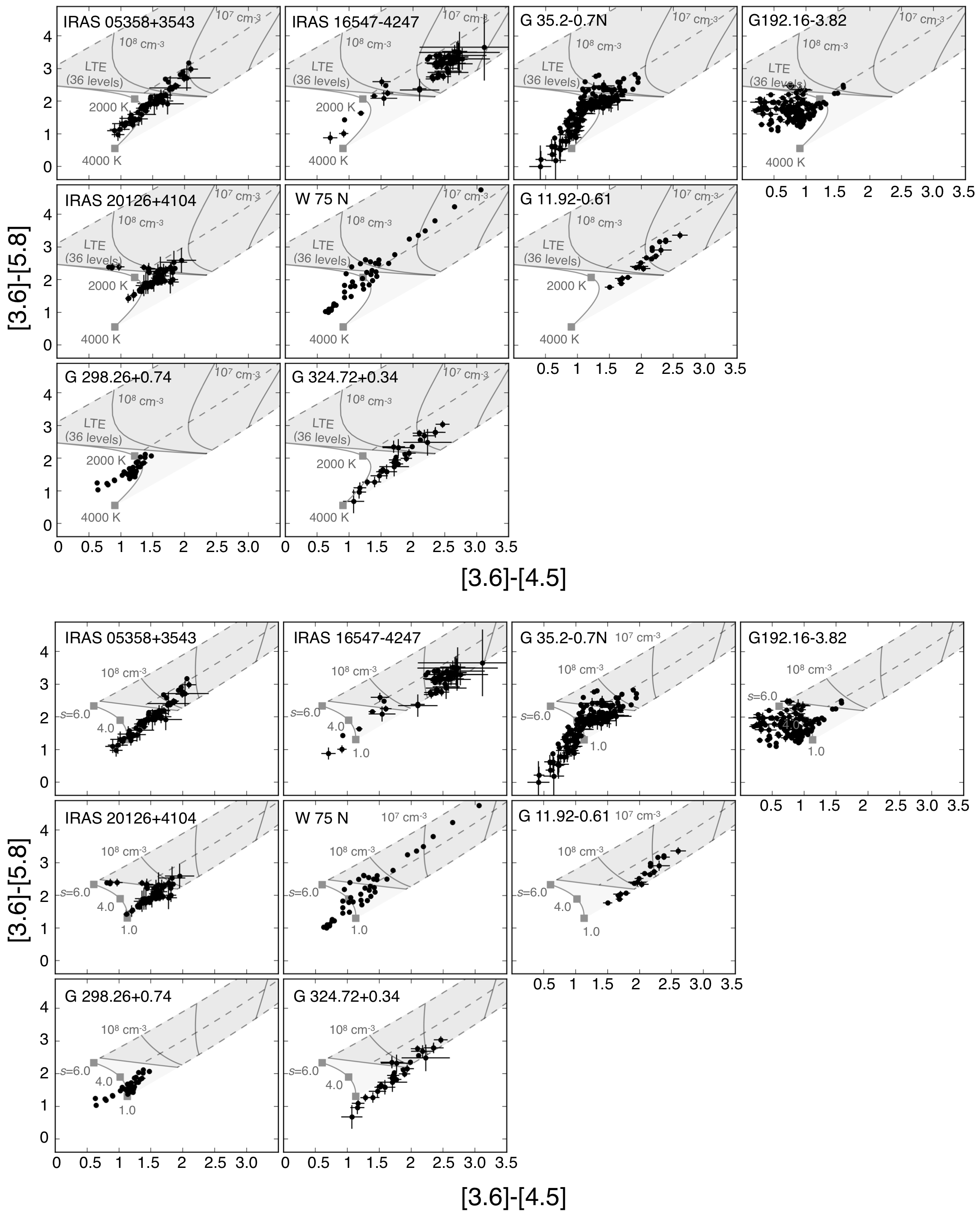
Figure 13: Same as Figure 5 but with diagrams for modeled thermal H₂ emission for collisions with H₂ and He shown in Figure 11.

In Figure 12 we plot the observed colors in Green Fuzzy emission with possible colors due to thermal H₂ as shown in Figure 11. While thermal H₂ could explain the colors observed at most of the positions, it cannot explain the colors with small [3.6]-[4.5] and [3.6]-[5.8] colors ($<$1.0 and $<$1.5, respectively) observed in IRAS 05358+3543, IRAS 16547–4247, G 35.2–0.7 N, G 192.16–3.82, W 75 N and G 298.26+0.74. These correspond to the regions with lowest 3.6/4.5- and 3.6/5.8-µm  flux ratios in Figure 4. Furthermore, thermal H₂ emission with H+He collisions cannot account for the large [3.6]-[4.5] and [3.6]-[5.8] colors ($>$2.1 and $>$2.6, respectively) in IRAS 16547–4247, W 75 N, G 11.92–0.61 and G 324.72+0.34. In Figure 13 we compare the linear correlation of the observed [3.6]-[4.5] and [3.6]-[5.8] colors with modeled thermal H₂ emission for collisions with H₂+He (Figure 11) in more detail. The figure shows that the linear correlation observed in Green Fuzzy emission may be attributed to different densities of gas observed in thermal H₂ emission. The problems with this explanation are discussed in Section 5 in detail.

4.3 PAH and fluorescent H₂ emission

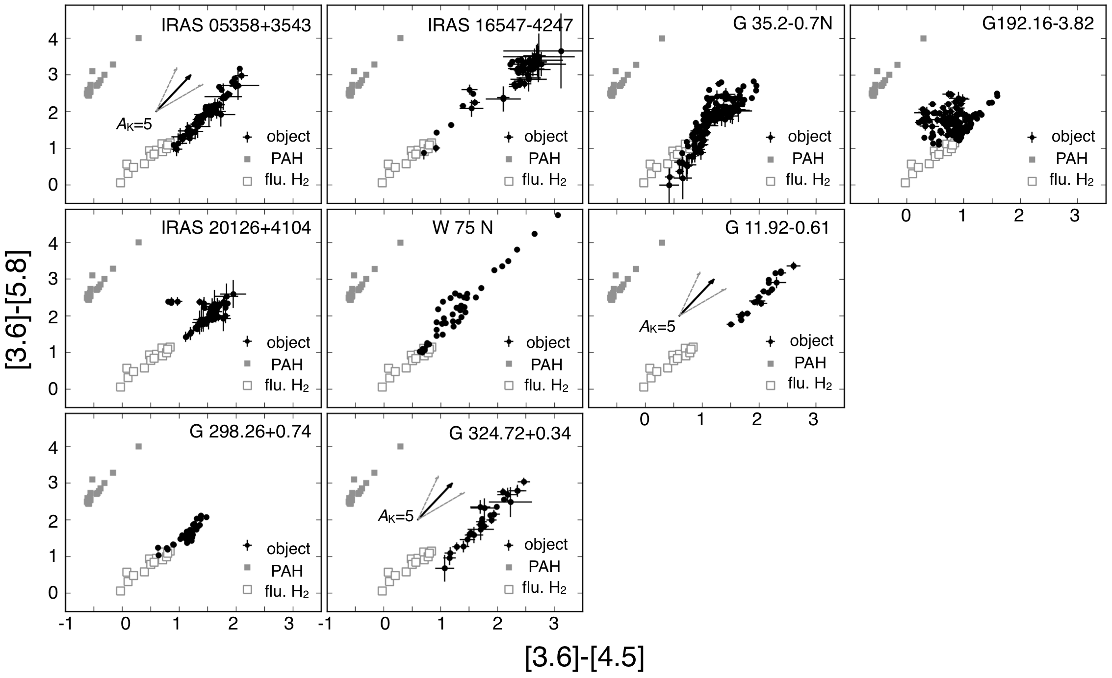
Figure 14: Same as Figure 4 but with models for PAH and fluorescent H₂ emission. See text for details of models.

Figure 14 shows color-color diagrams for the models of PAHs and fluorescent H₂ emission, usually associated with photodissociation regions (PDRs; e.g., Hollenbach and Tielens, 1997, for a review). Their fluxes are obtained from Draine and Li (2007) and Draine and Bertoldi (1996), respectively. The models by Draine and Li (2007) also include thermal dust continuum, which is prominently observed at longer wavelengths, but its contribution is negligible in the IRAC bands as compared with PAHs. For comparison we selected their results for a UV field 10²–10⁵ as large as the interstellar radiation field for the solar neighborhood. Such a UV field is comparable to those observed in well-known dense PDRs associated with OB stars such as Orion Bar, NGC 2023 and 7023 (e.g., Tielens, 2008; Usuda et al., 1996; Takami et al., 2000). For the abundance of PAH, all the results calculated for the dust/gas ratio in the Milky Way (fraction of C of 0.47–4.58 % to the entire abundance in the interstellar medium) are included in the figure.

In Figure 14 the colors for PAHs are noticeably offset from the linear correlation of [3.6]-[4.5] and [3.6]-[5.8] colors, with a combination of small [3.6]-[4.5] colors and large [3.6]-[5.8]. This indicates that PAHs are not primarily responsible for the color distribution observed in Green Fuzzy emission. In contrast, the constant [3.4]-[5.8] colors observed in several positions in IRAS 20126+4104 are similar to those of PAHs. The figure shows that the modeled colors for fluorescent H₂ show similar correlation between the [3.6]-[4.5] and [3.6]-[5.8] colors to those observed in most of Green Fuzzies. The discrepancy between the modeled and observed colors could be attributed to an extinction $A_{K}$ up to $\sim$20. This combination, however, cannot explain some pixels in G 35.2-0.7 N and G 324.72+0.34, with the lowest [3.6]-[4.5] and [3.6]-[5.8] colors. We discuss the possible contribution of fluorescent H₂ emission to the observed colors in detail in Section 5.3.

5 Discussion

5.1 Scattered continuum as a possible primary source of Green Fuzzy emission

The colors of the star+disk flux via scattering and extinction are approximately consistent with the observed colors. In particular, a similar correlation between [3.6]-[4.5] and [3.6]-[5.8] colors are observed in scattered continuum in the cavity of the L 1527 protostellar outflow, agreeing with this explanation. In this case, the color distribution observed in each object can be attributed to differing foreground extinctions (including dense cores and envelopes). This is corroborated by the facts that (1) the position of the protostar matches the regions with the lowest $I_{3.6~{}\micron}$/$I_{4.5~{}\micron}$ and $I_{3.6~{}\micron}$/$I_{5.8~{}\micron}$ ratios for most of the objects (Figure 4); and (2) the column density of the gas and dust is higher close to the protostar than in surrounding regions (see references for Table 2). This also suggests that the internal extinction in the extended emission regions is relatively small, otherwise the $I_{3.6~{}\micron}$/$I_{4.5~{}\micron}$ and $I_{3.6~{}\micron}$/$I_{5.8~{}\micron}$ ratios would decrease with increasing distance from the protostar due to reddening. In this context, the Green Fuzzy emission we analyzed may represent the morphology of cavities due to outflowing gas, and the $I_{3.6~{}\micron}$/$I_{4.5~{}\micron}$ and $I_{3.6~{}\micron}$/$I_{5.8~{}\micron}$ ratio maps in Figure 4 may represent the distribution of foreground extinction.

The explanation that Green Fuzzy emission is scattered continuum associated with outflow cavities is consistent with the fact their distribution is more similar to the 2-µm continuum than to the H₂ 2.12 µm  emission (Section 2). The morphological discrepancies between the 4.5-µm emission and continuum at 2 µm could be attributed to different extinctions at these wavelengths. This explanation is also consistent with the fact that such emission in some objects are associated with signatures of molecular outflows and/or outflow shocks (Section 2; see also Shepherd et al., 2007; Araya et al., 2007; Qiu et al., 2008; Cyganowski et al., 2009, 2011). It is intriguing that the distribution of the IRAC emission and/or 2-µm continuum do not match H₂ emission and/or molecular outflows in some objects, including IRAS 05358+3543, IRAS 16547–4247 and W 75 N (Section 2). This would indicate the complicated nature of high-mass star forming regions, which are often associated with multiple protostars and outflows like these objects (e.g., Shepherd et al., 2000, 2003; Beuther et al., 2002; Franco-Hernández et al., 2009).

As shown in Sections 3 and 4.2, some positions in G 192.16–3.82, G 35.2–0.7 N, and W 75 N show a [3.5]-[5.8] excess from the linear correlation of the [3.6]-[4.5] and [3.6]-[5.8] colors in the remaining region. This may be attributed to a different origin than scattered continuum. The deviation of the color observed in G 192.16–3.82 approximately matches the colors of PAHs in Figure 14, suggesting that this is due to diffuse contaminating PAH emission in the outer region where Green Fuzzy emission is relatively faint (Figure 6). This explanation is corroborated by the fact that the objects near G 192.16–3.82 are associated with extended emission at 8.0-µm (Figures 1 and 2), a signpost of PAH emission (Section 1). The same explanation may also apply to the [3.6]-[5.8] excess in W 75 N. This is corroborated by the fact that the region associated with the [3.6]-[5.8] excess is close to extended 8.0-µm emission (Figures 1 and 2) associated with an H II region (Haschick et al., 1981).

An alternative possible contributor for W 75 N and G 35.2–0.7 N is shocks the physical conditions of which are similar to some of those associated with low-mass protostars. This is consistent with the fact that the [3.6]-[5.8] excess in these objects is observed over color ranges similar to such shocks in Figure 10. Note that the fraction of the 4.5-µm flux in this component to that of the entire region (22, 34, 9 % for G 192.16–3.82, G 35.2–0.7 N, and W 75 N; Sections 3 and 4.2) is an upper limit for the additional emission component, assuming that the flux in the marked regions is solely due to shocks or PAHs. Throughout, the contaminating emission is a minor component in each object in terms of both spatial coverage and flux.

5.2 Thermal H₂ emission as a possible primary source of Green Fuzzy emission

As described in Section 1, H₂ or CO emission in shocks is often regarded as the primary source of Green Fuzzy emission (Rathborne et al., 2005; Araya et al., 2007; Shepherd et al., 2007; Qiu et al., 2008; Morales et al., 2009; Cyganowski et al., 2008, 2009, 2011; Chambers et al., 2009). Such emission is usually expected via thermal excitation. Indeed, thermal H₂ and CO emission explain well the IRAC colors observed in shocks associated with low-mass protostars (Ybarra and Lada, 2009; Takami et al., 2010). However, the [3.6]-[4.5] and [3.6]-[5.8] colors show different correlations between Green Fuzzy emission and these shocks associated with low-mass protostars (Section 4.1, Figure 10). This implies that different shock conditions are required if Green Fuzzy emission is due to shocks.

As described in Section 4, the Green Fuzzy emission in our sample does not show any clear signature for the presence of the ro-vibrational CO emission, which should only appear in the 4.5-µm band. In this subsection we therefore focus our discussion on thermal H₂ emission, which is primarily responsible for shocked H₂ emission in most cases (e.g., Brand et al., 1988; Gredel, 1994; Everett et al., 1995; Richter et al., 1995; Usuda et al., 1996; Eislöffel et al., 2000; Takami et al., 2006; Beck et al., 2008; Neufeld et al., 2006; Neufeld and Yuan, 2008; Neufeld et al., 2009). Indeed, the colors observed at most of the positions in Green Fuzzy emission are consistent with thermal H₂ emission (Section 4.1, Figure 12), which is primarily responsible for shocked H₂ emission. Furthermore, the linear correlation of the [3.6]-[4.5] and [3.6]-[5.8] colors may be attributed to different densities if thermal H₂ emission with H₂ and He collisions is responsible for the Green Fuzzy emission (Section 3.1, Figure 13).

These explanations, however, face several problems described below. First, in six out of nine objects (IRAS 05358+3543, IRAS 16547–4247, G 35.2–0.7 N, G192.16–3.82,W 75 N, G298.26-0.74), some positions show smaller [3.6]-[4.5] and [3.6]-[5.8] colors ($<$1.0 and $<$1.5, respectively) than those predicted by thermal H₂ emission (Section 4.1, Figure 12). In these objects the linear correlation between [3.6]-[4.5] and [3.6]-[5.8] is observed across both color ranges, suggestive of another origin. Secondly, Figures 12 and 13 would indicate the temperature of thermal H₂ is $\sim$2000 K, in which H₂ should be efficiently excited for the 1-0 S(1) 2.12 µm emission (e.g., Brand et al., 1988; Gredel, 1994; Everett et al., 1995; Richter et al., 1995; Usuda et al., 1996; Eislöffel et al., 2000; Takami et al., 2006; Beck et al., 2008; Neufeld et al., 2006; Neufeld and Yuan, 2008; Neufeld et al., 2009). It would therefore be puzzling if the distribution of Green Fuzzy emission were remarkably different from H₂ 2.12 µm emission (Section 2). See also Takami et al. (2010) for the dependence on density and temperature of H₂ emission at the 2.12 µm and IRAC bands.

Thirdly, if this color correlation is due to the different densities in Figure 13, it implies that the positions with larger [3.6]-[4.5] and [3.6]-[5.8] colors (thereby lower $I_{3.6\micron}/I_{4.5\micron}$ and $I_{3.6\micron}/I_{5.8\micron}$ flux ratios) are associated with lower densities. Since the $I_{3.6\micron}/I_{4.5\micron}$ and $I_{3.6\micron}/I_{5.8\micron}$ flux ratios increases with distance in G 35.2–0.7 N, G 192.16–3.82, W 75 N, the density should increase with distance in these objects. This is in the opposite sense as one would expect in outflow shocks. If these shocks are due to interaction between the ejecta and surrounding gas, as in many case (e.g., Bally et al., 2007; Arce et al., 2007), one would expect lower densities in the downstream as for the distribution of molecular gas around protostars (e.g., Stahler and Palla, 2005). If these shocks are in the ejecta, one would also expect such a density distribution as long as the flow has an opening angle similar to that observed in many molecular outflows (e.g., Beuther and Shepherd, 2005; Arce et al., 2007).

Fourthly, it is likely that the ro-vibrational CO emission significantly contributes to the entire 4.5-µm flux if the hydrogen number density exceeds $\sim 10^{7}$ cm^-3 (Neufeld and Yuan, 2008; Takami et al., 2010). This would cause larger [3.6]-[4.5] colors at high densities, as observed in colors in shocks associated with low-mass protostars at [3.6]-[5.8] $\sim$1.5-2.0 (Figure 10; see Takami et al., 2010, for details). However, such a tendency is not seen for the colors of Green Fuzzy emission in Figure 13.

Throughout, we conclude that it is not likely that Green Fuzzy emission is primarily due to thermal H₂ emission. One might think that a combination of thermal H₂ emission and scattered continuum could explain the linear correlation we have discussed. This explanation could overcome the first problem described above, interpreting the lowest [3.6]-[4.5] and [3.6]-[5.8] colors as scattered continuum. However, the second problem still remains. The third and fourth problems could only be overcome if the shock conditions were uniform, yielding a single combination of [3.6]-[4.5] and [3.6]-[5.8] colors over the region. This is not likely, considering the fact that shocks associated with high-mass protostellar outflows show complicated shock structures (see, e.g., Kaifu et al., 2000; Davis et al., 2007; Cunningham et al., 2009), suggesting the presence of different physical conditions in each outflow. It is noteworthy that, according to this explanation, we would expect scattered continuum further away from the protostar than H₂ emission (i.e., the regions with the largest $I_{3.6\micron}/I_{4.5\micron}$ and $I_{3.6\micron}/I_{5.8\micron}$) in G 35.2-0.7 N. This is the opposite trend as observed in the H₂ 2.12-µm emission and scattered continuum at 2 µm (Froebrich et al., 2011; Lee et al., 2012). There is no clear theory for how the above explanation overcomes this discrepancy.

Alternatively, a combination of thermal and fluorescent H₂ emission in shocks may explain the linear correlation in the color-color diagrams. We discuss this in the next subsection.

5.3 Fluorescent H₂

The linear correlation of the [3.6]-[4.5] and [3.6]-[5.8] colors may also be explained by a combination of fluorescent H₂ emission and extinction (Section 4.3). To investigate this possibility in detail, we calculate the IRAC fluxes expected for fluorescent H₂ in PDRs based on Draine and Bertoldi (1996). As for Section 4.3 and Figure 14, we selected their results for a UV field 10²–10⁵ as large as the interstellar radiation field for the solar neighborhood. Again, such a UV field is comparable to those observed in well-known dense PDRs associated with OB stars such as Orion Bar, NGC 2023 and 7023 (e.g., Tielens, 2008; Usuda et al., 1996; Takami et al., 2000). These are tabulated in Table 3. The table shows that the predicted fluxes are up to $\sim$3 MJy str^-1, significantly lower than those observed in the bright areas of the Green Fuzzy emission shown in Figure 1 ($\gg$ 10 MJy str^-1).

Furthermore, PDRs are also associated with the PAH emission, which appears to be much brighter in the 3–8 µm range (Tielens, 2008). To investigate this issue more quantitatively, we calculate the modeled fluxes for the same range of UV fields based on Draine and Li (2007). Draine and Li (2007) provide fluxes per column density, without the models for the PDRs. We therefore assume a column density for the PDRs of A_V=1, a typical column density for PDRs (e.g., Hollenbach and Tielens, 1997), corresponding to $1.9\times 10^{21}$ cm^-2 (Mathis, 2000). These are also tabulated in Table 3, for minimum and maximum abundances of PAHs modeled by Draine and Li (2007) ($q_{PAH}$=0.47 and 4.58 %, respectively). The larger $q_{PAH}$ value is comparable to those of well-studied dense PDRs ($\sim$3.5 %, Tielens, 2008). Table 3 shows that, even for the minimum abundance of PAH (i.e., lower than those of well studied dense PDRs by a factor of $\sim$7), the modeled PAH fluxes are larger than fluorescent H₂ by a factor of $>$6 and $>$100 at 3.6 and 5.8 µm, respectively. Thus, despite the uncertainty in the calculations (i.e., the column density of the PDRs), it is not likely that the fluorescent H₂ emission dominates over the PAH emissions in normal PDRs.

Fluorescent H₂ emission has been observed in the high-mass protostellar outflow DR 21 (Fernandes et al., 1997; Smith et al., 2006) and a well-known Herbig-Haro object (Fernandes and Brand, 1995). A combination of thermal and fluorescent H₂ may consistently explain the linear correlation of [3.6]-[4.5] and [3.6]-[5.8] colors observed in Green Fuzzy emission in most of the objects (Figures 12, 13, 14), if most of the PAHs+dust grains are destroyed by the passage of shocks. Fernandes et al. (1997) and Smith et al. (2006) suggested a UV field of H₂ excitation of $\chi\sim 10^{2}-10^{4}$ in the DR 21 outflow. Again, such a UV field would yield H₂ flux too low compared to the observations. This problem may be overcome if (1) most of the dust grains are destroyed by shocks, allowing UV photons to be absorbed more efficiently by molecular hydrogen; and/or (2) turbulence in the shocks make the ultraviolet H₂ lines broader, allowing more photons to be absorbed. Models for the coexistence of fluorescent and thermal H₂ in shocks are required to further investigate this possibility. Alternatively, follow-up spectroscopic observations of Green Fuzzy emission would allow us to further constrain the associated shock conditions.

5.4 PAHs

Our color-color diagrams show that PAHs are not the primary emission mechanism for Green Fuzzy emission (Section 4.3, Figure 14). In this section we discuss the cases for IRAS 20126+4104, in which a relatively constant [3.6]-[5.8] color is observed at several positions.

These positions in IRAS 20126+4104 show a relatively constant [3.6]-[5.8] color similar to PAHs (Section 4.3, Figure 14). While we do not reject the possibility that these emission components are primarily due to thermal H₂ (Section 4.1, Figures 12, 13), this coincidence suggests that at least their 3.6- and 5.8 µm  fluxes are primarily due to PAHs. However, the observed [3.6]-[4.5] colors in these regions are significantly larger than those of PAHs modeled by Draine and Li (2007), ranging from 0.8 to 1.5. This may be primarily due to a contribution from another emission mechanism at 4.5-µm, in which the PAHs emission is the faintest among the four IRAC bands (e.g., Reach et al., 2006; Draine and Li, 2007; Tielens, 2008, see also Table 3).

In IRAS 20126+4104, this emission component is associated with a point source to the west of the high-mass protostar (Section 3, Figure 6). The three-color image in Figure 2 shows the presence of excess emission at 8.0-µm, supporting the idea that this region is associated with PAH emission (Section 1). This region is surrounded by emission with different colors, which can be attributed to either scattered continuum (Section 5.1) or H₂ emission (Sections 5.2, 5.3). Thus, the different [3.6]-[4.5] colors described above can be naturally attributed to different contributions from two emission components (i.e., PAH and scattered continuum, or PAH and H₂ emission).

Four of our targets are associated with hypercompact and ultracompact H II regions (Table 2). Thus, these should also be associated with far-UV radiation which can excite PAHs. However, none of our targets show clear evidence for the presence of PAH emission directly associated with the protostar. These suggest that the high-mass protostars and hypercompact/ultracompact H II regions are heavily embedded even at the wavelengths of our analysis, i.e., 3.6–5.8 µm.

6 Caveats

It is beyond the scope of this paper to discuss the emission mechanisms below, but we briefly state their possible contributions.

Thermal dust continuum might also contribute to the 3.6-5.8 µm flux. Such emission can be extended in the outflow cavity (e.g., De Buizer, 2006). According to Draine and Li (2007) this emission component is negligible compared with PAH emission in the IRAC bands. However, the contribution from the thermal dust continuum may not be negligible in circumstances where PAHs are destroyed but larger grains survive.

Fast shocks should be associated with atomic and ionic lines, such as Pf $\gamma$ 3.74 µm, Br $\alpha$ 4.05 µm, Pf $\beta$ 4.65 µm, and Fe II 5.34 µm (Reach et al., 2006, see Table 1 for details), and these may also contribute to the 3.6-5.8 µm bands. In the limited cases discussed by Reach et al. (2006) the above lines in shocks yield $I_{3.6\micron}/I_{4.5\micron}$ and $I_{3.6\micron}/I_{5.8\micron}$ ratios of $\lesssim 0.1$, significantly lower than those observed in Green Fuzzies (Figure 4). Thus, this possibility should be addressed with more detailed modeling and/or spectroscopic observations.

7 Conclusions

We analyzed the flux ratios and pixel-pixel colors of “Green Fuzzy” emission toward six nearby ($d$=2–3 kpc) well-studied high-mass protostars and three candidate high-mass protorstars observed using the archival data for Spitzer IRAC at 3.6, 4.5, and 5.8 µm. In color-color diagrams most of the sources show a positive correlation between the [3.6]-[4.5] and [3.5]-[5.8] colors, in all or a part of the region, along the extinction vector. We compare them with the colors of other objects and models, i.e., (1) modeled scattered continuum, and observed scattered continuum associated with the L 1527 low-mass protostellar outflow; (2) shocks associated with low-mass protostars and modeled thermal H₂ emission; (3) modeled emission for fluorescent H₂ ; and (4) modeled emission for PAHs. The conclusions are as follows:-

1. Of the above emission mechanisms, scattered continuum in the outflow cavities provides the simplest explanation for the observed linear correlation. Indeed, such a correlation is also observed in the scattered continuum in L 1527. In this case, the different colors within each object are attributed to different degrees of foreground extinction at different positions in the extended emission. Different objects show different colors not only along the extinction vector, but also across it. This can be attributed to different intrinsic colors of the star(+disk) system between the objects. This interpretation, that scattered continuum is responsible for Green Fuzzy emission, is consistent with the fact that the distribution of emission is remarkably different from H₂ 2.12 µm emission in some objects, but more similar to the continuum at 2 µm.

2. The observed color correlation is remarkably different from that observed in molecular shocks in low-mass protostars, in which the emission is due to thermal H₂, plus CO at high densities. Even so, a significant fraction of the Green Fuzzy emission show colors within the color range of modeled thermal H₂ emission. However, this emission mechanism is not likely for the following reasons: (1) the observed linear correlation in some objects exceeds the color range predicted for thermal H₂; (2) while ro-vibrational CO emission should contribute to the 4.5-µm emission at high densities ($n_{H}\gtrsim 10^{7}$ cm ^-3), the observed color-color diagrams do not clearly show such a signature; (3) the temperature inferred by the color diagrams ($\sim$2000 K) would allow for H₂ 2.12µm emission to be observed, however, the distribution of this line emission does not match Green Fuzzy emission in some objects; and (4) higher densities in the outer region compared to the inner region are required to explain the color correlation in some objects, however, this is not likely.
   The first problem may be overcome if we attribute the lowest [3.6]-[4.5] and [3.6]-[5.8] colors to another origin, e.g., scattered continuum. However, a combination of thermal H₂ emission and scattered continuum does not seem to overcome the other problems described above.

3. Fluorescent H₂ in normal PDRs cannot account for the observed flux. Furthermore, emission from PAHs should dominate over fluorescent H₂ in the IRAC bands in such circumstances. Fluorescent H₂ in shocks may overcome these problems if shocks destroy PAHs and dust grains, and turbulence in shocks allows far-UV photons to be absorbed by H₂ more efficiently. A combination of fluorescent and thermal H₂ may also explain the observed linear correlation between [3.6]-[4.5] and [3.6]-[5.8] colors. Shock models with these excitation mechanisms are required to investigate the feasibility of this explanation.

4. As expected, our color-color diagrams show that PAHs are not the primary mechanism for Green Fuzzy emission. PAHs may significantly contribute in a part of the emission regions in another few objects including IRAS 20126+4104, G 192.16–3.82 and W 75 N. None of our sample show clear evidence for PAH emission directly associated with the high-mass protostars, several of which should be associated with ionizing radiation. This suggests that those protostars are heavily embedded even at mid-infrared.

In summary, among the emission mechanisms discussed above, scattered continuum in outflow cavities provides the simplest explanation for the observed linear correlation. Alternative possible emission mechanisms to explain the above linear correlation may be a combination of thermal and fluorescent H₂ emission in shocks, and a combination of scattered continuum and thermal H₂ emission, but detailed models or spectroscopic follow-up are required to further investigate this possibility. The first interpretation (i.e., attributing the Green Fuzzy emission to the scattered continuum in outflow cavities) does not change interpretations of some previous literature which show that Green Fuzzy emission is associated with signatures of jets and outflows (e.g., molecular outflows, shock tracer, or collimated ionized jet).

This work also highlights the difficulty in obtain definitive conclusions for the excitation mechanism of Green Fuzzies. Spectroscopic follow-up would allow us to complement this study in order to understand the nature of high-mass protostars themselves, or conditions of outflow shocks associated with high-mass protostars in detail.

Table 1: List of Lines in the IRAC Bands

Transition	$\lambda$ (µm)	$E_{u}/k$ ($\times 10^{3}$K )	IRAC Band
— Bright H2 lines —
1–0 $O$(5)	3.235	7.0	1
2–1 $O$(5)	3.438	12.6	1
1–0 $O$(6)	3.501	7.6	1
0–0 $S$(14)	3.724	19.4	1
1–0 $O$(7)	3.808	8.4	1
0–0 $S$(13)	3.846	17.4	1
0–0 $S$(12)	3.997	15.5	2
0–0 $S$(11)	4.181	13.7	2
0–0 $S$(10)	4.410	11.9	2
1–1 $S$(11)	4.417	19.0	2
0–0 $S$(9)	4.695	10.3	2
1–1 $S$(9)	4.953	15.7	2
0–0 $S$(8)	5.053	8.7	3
0–0 $S$(7)	5.511	7.2	3
0–0 $S$(6)	6.109	5.8	3
0–0 $S$(5)	6.909	4.6	4
1–1 $S$(5)	7.281	4.6	4
0–0 $S$(4)	8.026	3.5	4
0–0 $S$(3)	9.665	2.5	4
— Possible atomic and ionic lines in shocks —
Pf $\gamma$	3.741	155.3	1
Br $\gamma$	4.052	151.5	2
Pf $\beta$	4.654	154.6	2
Fe II	5.339	2.7	3
Ni II	6.636	2.2	4
Ar II	6.985	2.1	4
Pf $\alpha$	7.460	153.4	4
Ar III	8.991	1.6	4

Table 2: Target List

Object	Category	R.A. (2000)	Dec (2000)	Distance	Uncertainty of IRAC			Region selected for color-color
				(kpc)	flux (MJy str-1)			diagram
					3.6 µm	4.5 µm	5.8 µm
IIRAS 05358+3543	HPMO	5h 39m 13.0s	35∘ 45’ 51”	1.8	0.44	0.53	0.99	$>$15-$\sigma$ for 4.5 µm
IRAS 16547–4247	HPMO	16h 58m 17.2s	–42∘ 52’ 08”	2.9	0.67	0.98	1.44	$>$15-$\sigma$ for 4.5 µm
G 35.2–0.7 N	HC HII	18h 58m 13.0s	1∘ 40’ 36”	$\sim$2	0.36	0.42	0.87	$>$15-$\sigma$ for 4.5 µm
G 192.16–3.82	HC HII	5h 58m 13.5s	16∘ 31’ 58”	$\sim$2	0.14	0.16	0.46	$>$15-$\sigma$ for 4.5 µm
IRAS 20126+4104	HC HII	20h 14m 26.0s	41∘ 13’ 33”	1.7	0.50	0.94	3.45	$>$15-$\sigma$ for 4.5 µm, $>$5-$\sigma$ for 5.8 µm
W 75 N	UC HII	20h 38m 36.4s	42∘ 37’ 34”	$\sim$2	0.28	0.19	0.57	$>1.0\times 10^{2}$ MJy str-1 for 4.5 µm
G 11.92–0.61	C08	18h 13m 58.1s	–18∘ 54’ 17”	3.8	0.43	1.24	0.77	$>$15-$\sigma$ for 4.5 µm
G 298.26+0.74	C08	12h 11m 47.7s	–61∘ 46’ 21”	—	0.23	0.22	0.24	$>$80-$\sigma$ for 4.5 µm
G 324.72+0.34	C08	15h 34m 57.5s	–55∘ 27’ 26”	—	0.20	0.28	0.40	$>$15-$\sigma$ for 4.5 µm

Table 3: IRAC Flux Estimated for fluorescent H₂ and PAHs (MJy str^-1)

	Fluorescent H2							PAH
$\chi$	$T_{0}$	$n_{H}$						$q_{PAH}$=0.47					$q_{PAH}$=4.58
	(K)	(cm-3)	3.6 µm	4.5 µm	5.8 µm	8.0 µm		3.6 µm	4.5 µm	5.8 µm	8.0 µm		3.6 µm	4.5 µm	5.8 µm	8.0 µm
1.0$\times 10^{2}$	1000	1.0$\times 10^{3}$	0.03	0.02	0.01	0.10		0.25	8.7$\times 10^{-2}$	0.96	4.3		3.2	1.1	11	38
1.0$\times 10^{2}$	500	1.0$\times 10^{3}$	0.02	0.01	$<$0.01	0.01		0.25	8.7$\times 10^{-2}$	0.96	4.3		3.2	1.1	11	38
1.0$\times 10^{2}$	300	1.0$\times 10^{4}$	0.03	0.02	0.01	0.01		0.25	8.7$\times 10^{-2}$	0.96	4.3		3.2	1.1	11	38
1.0$\times 10^{2}$	500	1.0$\times 10^{4}$	0.04	0.02	0.01	0.04		0.25	8.7$\times 10^{-2}$	0.96	4.3		3.2	1.1	11	38
1.0$\times 10^{3}$	1000	1.0$\times 10^{4}$	0.21	0.16	0.08	0.70		2.5	0.89	11	62		32	11	1.2$\times 10^{2}$	4.0$\times 10^{2}$
1.0$\times 10^{3}$	500	1.0$\times 10^{4}$	0.18	0.13	0.05	0.06		2.5	0.89	11	62		32	11	1.2$\times 10^{2}$	4.0$\times 10^{2}$
1.0$\times 10^{3}$	300	1.0$\times 10^{5}$	0.27	0.21	0.10	0.09		2.5	0.89	11	62		32	11	1.2$\times 10^{2}$	4.0$\times 10^{2}$
1.0$\times 10^{3}$	500	1.0$\times 10^{5}$	0.26	0.23	0.11	0.27		2.5	0.89	11	62		32	11	1.2$\times 10^{2}$	4.0$\times 10^{2}$
1.0$\times 10^{4}$	1000	1.0$\times 10^{5}$	0.98	0.94	0.48	1.73		26	9.9	1.7$\times 10^{2}$	1.3$\times 10^{3}$		3.3$\times 10^{2}$	1.2$\times 10^{2}$	1.3$\times 10^{3}$	4.8$\times 10^{3}$
1.0$\times 10^{4}$	500	1.0$\times 10^{5}$	1.01	0.86	0.38	0.37		26	9.9	1.7$\times 10^{2}$	1.3$\times 10^{3}$		3.3$\times 10^{2}$	1.2$\times 10^{2}$	1.3$\times 10^{3}$	4.8$\times 10^{3}$
1.0$\times 10^{4}$	300	1.0$\times 10^{6}$	1.22	1.19	0.49	0.29		26	9.9	1.7$\times 10^{2}$	1.3$\times 10^{3}$		3.3$\times 10^{2}$	1.2$\times 10^{2}$	1.3$\times 10^{3}$	4.8$\times 10^{3}$
1.0$\times 10^{4}$	500	1.0$\times 10^{6}$	1.07	1.12	0.46	0.52		26	9.9	1.7$\times 10^{2}$	1.3E+09		3.3$\times 10^{2}$	1.2$\times 10^{2}$	1.3$\times 10^{3}$	4.8$\times 10^{3}$
1.0$\times 10^{5}$	1000	1.0$\times 10^{6}$	2.61	2.88	1.32	2.32		3.3$\times 10^{2}$	2.6$\times 10^{2}$	5.0$\times 10^{3}$	3.1$\times 10^{4}$		3.8$\times 10^{3}$	1.5$\times 10^{3}$	1.7$\times 10^{4}$	6.6$\times 10^{4}$
1.0$\times 10^{5}$	500	1.0$\times 10^{6}$	3.03	3.20	1.43	0.94		3.3$\times 10^{2}$	2.6$\times 10^{2}$	5.0$\times 10^{3}$	3.1$\times 10^{4}$		3.8$\times 10^{3}$	1.5$\times 10^{3}$	1.7$\times 10^{4}$	6.6$\times 10^{4}$

References

- Araya et al. (2007) Araya, E., Hofner, P., Sewiło, M., Goss, W. M., Linz, H., Kurtz, S., Olmi, L., Churchwell, E., Rodríguez, L. F., and Garay, G.: 2007, ApJ 669, 1050
- Arce et al. (2007) Arce, H. G., Shepherd, D., Gueth, F., Lee, C., Bachiller, R., Rosen, A., and Beuther, H.: 2007, Protostars and Planets V pp 245–260
- Bally et al. (2007) Bally, J., Reipurth, B., and Davis, C. J.: 2007, Protostars and Planets V pp 215–230
- Beck et al. (2008) Beck, T. L., McGregor, P. J., Takami, M., and Pyo, T.: 2008, ApJ 676, 472
- Beuther et al. (2007) Beuther, H., Churchwell, E. B., McKee, C. F., and Tan, J. C.: 2007, Protostars and Planets V pp 165–180
- Beuther et al. (2002) Beuther, H., Schilke, P., Gueth, F., McCaughrean, M., Andersen, M., Sridharan, T. K., and Menten, K. M.: 2002, A&A 387, 931
- Beuther and Shepherd (2005) Beuther, H. and Shepherd, D.: 2005, in M. S. N. Kumar, M. Tafalla, & P. Caselli (ed.), Cores to Clusters: Star Formation with Next Generation Telescopes, pp 105–119
- Brand et al. (1988) Brand, P. W. J. L., Moorhouse, A., Burton, M. G., Geballe, T. R., Bird, M., and Wade, R.: 1988, ApJ 334, L103
- Brooks et al. (2003) Brooks, K. J., Garay, G., Mardones, D., and Bronfman, L.: 2003, ApJ 594, L131
- Cesaroni et al. (1999) Cesaroni, R., Felli, M., Jenness, T., Neri, R., Olmi, L., Robberto, M., Testi, L., and Walmsley, C. M.: 1999, A&A 345, 949
- Cesaroni et al. (2007) Cesaroni, R., Galli, D., Lodato, G., Walmsley, C. M., and Zhang, Q.: 2007, Protostars and Planets V pp 197–212
- Chambers et al. (2009) Chambers, E. T., Jackson, J. M., Rathborne, J. M., and Simon, R.: 2009, ApJS 181, 360
- Chapman et al. (2009) Chapman, N. L., Mundy, L. G., Lai, S., and Evans, N. J.: 2009, ApJ 690, 496
- Cunningham et al. (2009) Cunningham, N. J., Moeckel, N., and Bally, J.: 2009, ApJ 692, 943
- Cyganowski et al. (2009) Cyganowski, C. J., Brogan, C. L., Hunter, T. R., and Churchwell, E.: 2009, ApJ 702, 1615
- Cyganowski et al. (2011) Cyganowski, C. J., Brogan, C. L., Hunter, T. R., Churchwell, E., and Zhang, Q.: 2011, ApJ 729, 124
- Cyganowski et al. (2008) Cyganowski, C. J., Whitney, B. A., Holden, E., Braden, E., Brogan, C. L., Churchwell, E., Indebetouw, R., Watson, D. F., Babler, B. L., Benjamin, R., Gomez, M., Meade, M. R., Povich, M. S., Robitaille, T. P., and Watson, C.: 2008, AJ 136, 2391
- Davis et al. (2007) Davis, C. J., Kumar, M. S. N., Sandell, G., Froebrich, D., Smith, M. D., and Currie, M. J.: 2007, MNRAS 374, 29
- Davis et al. (1998) Davis, C. J., Moriarty-Schieven, G., Eislöffel, J., Hoare, M. G., and Ray, T. P.: 1998, AJ 115, 1118
- De Buizer (2006) De Buizer, J. M.: 2006, ApJ 642, L57
- De Buizer and Vacca (2010) De Buizer, J. M. and Vacca, W. D.: 2010, AJ 140, 196
- Draine and Bertoldi (1996) Draine, B. T. and Bertoldi, F.: 1996, ApJ 468, 269
- Draine and Li (2007) Draine, B. T. and Li, A.: 2007, ApJ 657, 810
- Eislöffel et al. (2000) Eislöffel, J., Smith, M. D., and Davis, C. J.: 2000, A&A 359, 1147
- Everett et al. (1995) Everett, M. E., Depoy, D. L., and Pogge, R. W.: 1995, AJ 110, 1295
- Fernandes and Brand (1995) Fernandes, A. J. L. and Brand, P. W. J. L.: 1995, MNRAS 274, 639
- Fernandes et al. (1997) Fernandes, A. J. L., Brand, P. W. J. L., and Burton, M. G.: 1997, MNRAS 290, 216
- Franco-Hernández et al. (2009) Franco-Hernández, R., Moran, J. M., Rodríguez, L. F., and Garay, G.: 2009, ApJ 701, 974
- Froebrich et al. (2011) Froebrich, D., Davis, C. J., Ioannidis, G., Gledhill, T. M., Takami, M., Chrysostomou, A., Drew, J., Eislöffel, J., Gosling, A., Gredel, R., Hatchell, J., Hodapp, K. W., Kumar, M. S. N., Lucas, P. W., Matthews, H., Rawlings, M. G., Smith, M. D., Stecklum, B., Varricatt, W. P., Lee, H. T., Teixeira, P. S., Aspin, C., Khanzadyan, T., Karr, J., Kim, H.-J., Koo, B.-C., Lee, J. J., Lee, Y.-H., Magakian, T. Y., Movsessian, T. A., Nikogossian, E. H., Pyo, T. S., and Stanke, T.: 2011, MNRAS 413, 480
- Gibb et al. (2003) Gibb, A. G., Hoare, M. G., Little, L. T., and Wright, M. C. H.: 2003, MNRAS 339, 1011
- Gredel (1994) Gredel, R.: 1994, A&A 292, 580
- Haschick et al. (1981) Haschick, A. D., Reid, M. J., Burke, B. F., Moran, J. M., and Miller, G.: 1981, ApJ 244, 76
- Hollenbach and McKee (1989) Hollenbach, D. and McKee, C. F.: 1989, ApJ 342, 306
- Hollenbach and Tielens (1997) Hollenbach, D. J. and Tielens, A. G. G. M.: 1997, ARA&A 35, 179
- Indebetouw et al. (2003) Indebetouw, R., Watson, C., Johnson, K. E., Whitney, B., and Churchwell, E.: 2003, ApJ 596, L83
- Kaifu et al. (2000) Kaifu, N., Usuda, T., Hayashi, S. S., Itoh, Y., Akiyama, M., Yamashita, T., Nakajima, Y., Tamura, M., Inutsuka, S., Hayashi, M., Maihara, T., Iwamuro, F., Motohara, K., Iwai, J., Tanabe, H., Taguchi, T., Hata, R., Terada, H., Goto, M., Ando, H., Aoki, T., Chikada, Y., Doi, M., Ebizuka, N., Fukuda, T., Hamabe, M., Hasegawa, T., Horaguchi, T., Ichikawa, S., Ichikawa, T., Imanishi, M., Imi, K., Inata, M., Isobe, S., Iye, M., Kamata, Y., Kanzawa, T., Karoji, H., Kashikawa, N., Kataza, H., Kato, T., Kobayashi, N., Kobayashi, Y., Kodaira, K., Kosugi, G., Kurakami, T., Mikami, Y., Miyama, S. M., Miyashita, A., Miyata, T., Miyazaki, S., Mizumoto, Y., Nakagiri, M., Nakajima, K., Nakamura, K., Nariai, K., Nishihara, E., Nishikawa, J., Nishimura, S., Nishimura, T., Nishino, T., Noguchi, K., Noguchi, T., Noumaru, J., Ogasawara, R., Okada, N., Okita, K., Omata, K., Oshima, N., Otsubo, M., Sasaki, G., Sasaki, T., Sekiguchi, M., Sekiguchi, K., Shelton, I., Simpson, C., Suto, H., Takami, H., Takata, T., Takato, N., Tanaka, K., Tanaka, W., Tomono, D., Torii, Y., Waseda, K., Watanabe, J., Watanabe, M., Yagi, M., Yamashita, Y., Yasuda, N., Yoshida, M., Yoshida, S., and Yutani, M.: 2000, PASJ 52, 1
- Kim et al. (1994) Kim, S., Martin, P. G., and Hendry, P. D.: 1994, ApJ 422, 164
- Kumar and Grave (2007) Kumar, M. S. N. and Grave, J. M. C.: 2007, A&A 472, 155
- Laor and Draine (1993) Laor, A. and Draine, B. T.: 1993, ApJ 402, 441
- Le Bourlot et al. (1999) Le Bourlot, J., Pineau des Forêts, G., and Flower, D. R.: 1999, MNRAS 305, 802
- Lee et al. (2012) Lee, H.-T. , Takami, M., Duan, H.-Y., Karr, J.L., Su, Y.-N., Froebrich, D., Yeh, C.: 2012, ApJ submitted
- Lepp and McCray (1983) Lepp, S. and McCray, R.: 1983, ApJ 269, 560
- Marston et al. (2004) Marston, A. P., Reach, W. T., Noriega-Crespo, A., Rho, J., Smith, H. A., Melnick, G., Fazio, G., Rieke, G., Carey, S., Rebull, L., Muzerolle, J., Egami, E., Watson, D. M., Pipher, J. L., Latter, W. B., and Stapelfeldt, K.: 2004, ApJS 154, 333
- Mathis (2000) Mathis, J. S.: 2000, Circumstellar and Interstellar Material, pp 523–+
- Morales et al. (2009) Morales, E. F. E., Mardones, D., Garay, G., Brooks, K. J., and Pineda, J. E.: 2009, ApJ 698, 488
- Neufeld et al. (2006) Neufeld, D. A., Melnick, G. J., Sonnentrucker, P., Bergin, E. A., Green, J. D., Kim, K. H., Watson, D. M., Forrest, W. J., and Pipher, J. L.: 2006, ApJ 649, 816
- Neufeld et al. (2009) Neufeld, D. A., Nisini, B., Giannini, T., Melnick, G. J., Bergin, E. A., Yuan, Y., Maret, S., Tolls, V., Güsten, R., and Kaufman, M. J.: 2009, ApJ 706, 170
- Neufeld and Yuan (2008) Neufeld, D. A. and Yuan, Y.: 2008, ApJ 678, 974
- Noriega-Crespo et al. (2004) Noriega-Crespo, A., Morris, P., Marleau, F. R., Carey, S., Boogert, A., van Dishoeck, E., Evans, II, N. J., Keene, J., Muzerolle, J., Stapelfeldt, K., Pontoppidan, K., Lowrance, P., Allen, L., and Bourke, T. L.: 2004, ApJS 154, 352
- Qiu et al. (2008) Qiu, K., Zhang, Q., Megeath, S. T., Gutermuth, R. A., Beuther, H., Shepherd, D. S., Sridharan, T. K., Testi, L., and De Pree, C. G.: 2008, ApJ 685, 1005
- Rathborne et al. (2005) Rathborne, J. M., Jackson, J. M., Chambers, E. T., Simon, R., Shipman, R., and Frieswijk, W.: 2005, ApJ 630, L181
- Reach et al. (2006) Reach, W. T., Rho, J., Tappe, A., Pannuti, T. G., Brogan, C. L., Churchwell, E. B., Meade, M. R., Babler, B., Indebetouw, R., and Whitney, B. A.: 2006, AJ 131, 1479
- Richter et al. (1995) Richter, M. J., Graham, J. R., and Wright, G. S.: 1995, ApJ 454, 277
- Robitaille et al. (2006) Robitaille, T. P., Whitney, B. A., Indebetouw, R., Wood, K., and Denzmore, P.: 2006, ApJS 167, 256
- Shakura and Sunyaev (1973) Shakura, N. I. and Sunyaev, R. A.: 1973, A&A 24, 337
- Shepherd et al. (2001) Shepherd, D. S., Claussen, M. J., and Kurtz, S. E.: 2001, Science 292, 1513
- Shepherd et al. (2007) Shepherd, D. S., Povich, M. S., Whitney, B. A., Robitaille, T. P., Nürnberger, D. E. A., Bronfman, L., Stark, D. P., Indebetouw, R., Meade, M. R., and Babler, B. L.: 2007, ApJ 669, 464
- Shepherd et al. (2003) Shepherd, D. S., Testi, L., and Stark, D. P.: 2003, ApJ 584, 882
- Shepherd et al. (1998) Shepherd, D. S., Watson, A. M., Sargent, A. I., and Churchwell, E.: 1998, ApJ 507, 861
- Shepherd et al. (2000) Shepherd, D. S., Yu, K. C., Bally, J., and Testi, L.: 2000, ApJ 535, 833
- Simpson et al. (2009) Simpson, J. P., Burton, M. G., Colgan, S. W. J., Cotera, A. S., Erickson, E. F., Hines, D. C., and Whitney, B. A.: 2009, ApJ 700, 1488
- Smith et al. (2006) Smith, H. A., Hora, J. L., Marengo, M., and Pipher, J. L.: 2006, ApJ 645, 1264
- Smith and Rosen (2005) Smith, M. D. and Rosen, A.: 2005, MNRAS 357, 579
- Sollins et al. (2004) Sollins, P. K., Hunter, T. R., Battat, J., Beuther, H., Ho, P. T. P., Lim, J., Liu, S. Y., Ohashi, N., Sridharan, T. K., Su, Y. N., Zhao, J., and Zhang, Q.: 2004, ApJ 616, L35
- Stahler and Palla (2005) Stahler, S. W. and Palla, F.: 2005, The Formation of Stars
- Takami et al. (2006) Takami, M., Chrysostomou, A., Ray, T. P., Davis, C. J., Dent, W. R. F., Bailey, J., Tamura, M., Terada, H., and Pyo, T. S.: 2006, ApJ 641, 357
- Takami et al. (2010) Takami, M., Karr, J. L., Koh, H., Chen, H., and Lee, H.: 2010, ApJ 720, 155
- Takami et al. (2000) Takami, M., Usuda, T., Sugai, H., Kawabata, H., Suto, H., and Tanaka, M.: 2000, ApJ 529, 268
- Teixeira et al. (2008) Teixeira, P. S., McCoey, C., Fich, M., and Lada, C. J.: 2008, MNRAS 384, 71
- Tielens (2008) Tielens, A. G. G. M.: 2008, ARA&A 46, 289
- Tobin et al. (2008) Tobin, J. J., Hartmann, L., Calvet, N., and D’Alessio, P.: 2008, ApJ 679, 1364
- Tobin et al. (2007) Tobin, J. J., Looney, L. W., Mundy, L. G., Kwon, W., and Hamidouche, M.: 2007, ApJ 659, 1404
- Usuda et al. (1996) Usuda, T., Sugai, H., Kawabata, H., Inoue, M. Y., Kataza, H., and Tanaka, M.: 1996, ApJ 464, 818
- Varricatt (2011) Varricatt, W. P.: 2011, A&A 527, A97+
- Varricatt et al. (2010) Varricatt, W. P., Davis, C. J., Ramsay, S., and Todd, S. P.: 2010, MNRAS 404, 661
- Whitney et al. (2003a) Whitney, B. A., Wood, K., Bjorkman, J. E., and Cohen, M.: 2003a, ApJ 598, 1079
- Whitney et al. (2003b) Whitney, B. A., Wood, K., Bjorkman, J. E., and Wolff, M. J.: 2003b, ApJ 591, 1049
- Wolniewicz et al. (1998) Wolniewicz, L., Simbotin, I., and Dalgarno, A.: 1998, ApJS 115, 293
- Wrathmall et al. (2007) Wrathmall, S. A., Gusdorf, A., and Flower, D. R.: 2007, MNRAS 382, 133
- Ybarra and Lada (2009) Ybarra, J. E. and Lada, E. A.: 2009, ApJ 695, L120
- Zhang and Wang (2009) Zhang, M. and Wang, H.: 2009, AJ 138, 1830