Long-range corrected hybrid meta-generalized-gradient approximations with dispersion corrections

Abstract

We propose a long-range corrected hybrid meta-GGA functional, based on a global hybrid meta-GGA functional, M05 [Y. Zhao, N. E. Schultz, and D. G. Truhlar, J. Chem. Phys. 123, 161103 (2005)], and empirical atom-atom dispersion corrections. Our resulting functional, $\omega\text{M05-D}$, is shown to be accurate for a very wide range of applications, such as thermochemistry, kinetics, noncovalent interactions, equilibrium geometries, frontier orbital energies, fundamental gaps, and excitation energies. In addition, we present three new databases, IP131 (131 ionization potentials), EA115 (115 electron affinities), and FG115 (115 fundamental gaps), consisting of experimental molecular geometries and accurate reference values, which will be useful in the assessment of the accuracy of density functional approximations.

I Introduction

Because of its satisfactory accuracy and modest cost in many applications, Kohn-Sham density functional theory (KS-DFT) Hohenberg and Kohn (1964); Kohn and Sham (1965) has become one of the most popular electronic structure methods for large ground-state systems Parr and Yang (1989); Dreizler and Gross (1990); Engel and Dreizler (2011); Kohn et al. (1996). Its extension for treating excited-state systems, time-dependent density functional theory (TDDFT) Casida (1995); Gross et al. (1996), has also been widely used.

The crucial ingredient of KS-DFT, the exact exchange-correlation (XC) energy functional $E_{xc}[\rho]$, however, remains unknown and needs to be approximated. Functionals based on the local density approximation (LDA), modeling the XC energy density locally with that of a uniform electron gas (UEG), have been quite successful for nearly-free electron systems Parr and Yang (1989); Dreizler and Gross (1990), though still insufficiently accurate for most quantum chemical applications. Functionals based on the generalized gradient approximations (GGAs), additionally incorporating the gradient of local density into the LDA, have achieved reasonable accuracy in many applications. As an extension of the GGA (for rather restricted set of density variables), meta-GGA (MGGA) offers itself quite naturally. Functionals depending directly on the Laplacian of the density have not been pursued intensively, because of the difficulty of numerical evaluation. MGGAs, which adopt the kinetic energy density as a substitute for the Laplacian, have shown evidences of superiority over GGAs. Voorhis and Scuseria (1998); Tao et al. (2003); Zhao and Truhlar (2006)

However, the LDA, GGAs and MGGAs (commonly denoted as DFAs for density functional approximations) are based on the localized model XC holes, while the exact XC hole should be fully nonlocal. Currently, perhaps the most successful approaches to taking into account the nonlocality of XC hole are provided by hybrid DFT methods, incorporating a fraction of the exact Hartree-Fock (HF) exchange into the DFAs. Hybrid density functionals have achieved remarkable accuracy and have expanded the usefulness of DFT for many applications. Noticeably, global hybrid MGGA functionals Becke (1996); Boese and Handy (2002); Staroverov et al. (2003); Zhao et al. (2004); Hill et al. (2006); Boese and Martin (2004); Zhao et al. (2005a, 2006a); Zhao and Truhlar (2008a), where the XC energy density depends on the local density, the gradient of local density, a fraction of exact exchange, as well as the exact KS kinetic energy density (a function of the occupied KS orbitals) Becke (1983, 1998, 2000); Schmider and Becke (2000), have been shown to potentially perform better than global hybrid GGA functionals Zhao et al. (2004); Hill et al. (2006); Boese and Martin (2004); Zhao et al. (2005a, 2006a); Zhao and Truhlar (2008a, b, c), due to the additional ingredient of kinetic energy density in global hybrid MGGA functionals.

In global hybrid functionals, a small fraction of the exact HF exchange is added to a semilocal density functional. In certain situations, especially in the asymptotic regions of molecular systems, a large fraction (even 100%) of HF exchange is needed. Aiming to remedy this, long-range corrected (LC) hybrid DFT schemes have been actively developed Iikura et al. (2001); Tawada et al. (2004); Gerber and $\acute{\text{A}}$ngy$\acute{\text{a}}$n (2005); Gerber et al. (2007); Vydrov et al. (2006); Vydrov and Scuseria (2006); Song et al. (2007); Cohen et al. (2007); Chai and Head-Gordon (2008a, b, 2009). LC hybrids retain the full HF exchange only for the long-range electron-electron interactions, and thereby resolve a significant part of the self-interaction problems associated with global hybrid functionals.

On the other hand, the development of accurate short-range (SR) exchange density functionals $E_{x}^{\text{SR}}[\rho]$, plays an important role in the progress of LC-DFT. In the first LC scheme, an ansatz for the conversion of any $E_{x}$ to $E_{x}^{\text{SR}}$ was proposed by Iikura et al. Iikura et al. (2001), and has become widely used. However, their resulting LC hybrid GGA functionals do not outperform the corresponding global hybrid GGA functionals for thermochemistry. In 2006, Vydrov et al. proposed a different LC scheme Vydrov et al. (2006), based on integrating a GGA model exchange hole. Their resulting LC-$\omega$PBE functional has shown improved performance for thermochemistry and barrier heights, and is comparable to global hybrid GGA functionals such as B3LYP Becke (1993); Stephens et al. (1994). However, further improvements following this direction require the development of more accurate model exchange holes, which is a quite challenging task.

Another approach to more accurate LC hybrid functionals was proposed by Chai and Head-Gordon Chai and Head-Gordon (2008a). First, augmenting the SR local spin density exchange energy density by a flexible enhancement factor (of the Becke’s 1997 form Becke (1997)) and fully reoptimizing the LC functional on a diverse training set, yields the $\omega$B97 functional. Second, including an adjustable fraction of SR HF exchange in the $\omega$B97 functional with the similar reoptimization procedure, leads to the $\omega$B97X functional. $\omega$B97 and $\omega$B97X have been shown to be accurate across a diverse set of test data, containing thermochemistry, kinetics, and noncovalent interactions Chai and Head-Gordon (2008a).

However, problems associated with the lack of nonlocality of the DFA correlation hole, such as the lack of dispersion interactions (the missing of van der Waals forces), are not resolved by the LC hybrid schemes. The correlation functionals in typical LC hybrids are treated semilocally, which cannot capture the long-range (LR) correlation effects Dobson et al. (2001); Kristyan and Pulay (1994). To remedy this, the DFT-D scheme was applied Wu et al. (2001); *Wu02; *Zimmerli04; *Grimme04; *Grimme06; *Antony06; *Jurecka06; *Goursot07; *Grimme07; *Cerny07; *Morgado07; *Kabelac07; *Cerny_PCCP07 to extend the $\omega$B97X functional with damped atom-atom dispersion corrections, denoted as $\omega$B97X-D Chai and Head-Gordon (2008b). Consequently, $\omega$B97X-D can obtain dispersive effects with essentially zero additional computational cost relative to $\omega$B97X. As an alternative approach, $\omega$B97X has also been combined with the double-hybrid methods Grimme (2006b); Schwabe and Grimme (2007); Tarnopolsky et al. (2008); Benighaus et al. (2008); Zhang et al. (2009), which mix both the HF exchange and nonlocal orbital correlation energy from the second-order perturbation energy expression in wave function theory. The resulting $\omega$B97X-2 functional Chai and Head-Gordon (2009) has yielded very high accuracy for thermochemistry, kinetics, and noncovalent interactions, though its fifth-order scaling with respect to system size may limit its applicability to larger systems.

As the $\omega$B97 series are LC hybrid GGAs, it seems a natural step to develop LC hybrid MGGAs and to assess their performance. In this work, we propose a new LC hybrid MGGA-D functional, denoted as $\omega\text{M05-D}$, which is shown to be accurate for a wide range of applications, when compared with the two closely related functionals: a global hybrid MGGA functional (M05-2X) Zhao et al. (2006a) and a LC hybrid GGA-D functional ($\omega$B97X-D) Chai and Head-Gordon (2008b). The rest of this paper is organized as follows. In Sec. II, we briefly describe the relevant schemes developed in the LC hybrid approach. In Sec. III, we propose a new SR exchange functional, which serves as suitable basis functionals for systematically generating accurate LC hybrid MGGA functionals. The performance of the $\omega\text{M05-D}$ functional is compared with other functionals in Sec. IV (on the training set), and in Sec. V (on some test sets). In Sec. VI, we give our conclusions.

II Rationales of LC Hybrid Schemes

For the LC hybrid schemes, one first defines the long-range and short-range operators to partition the Coulomb operator. The most popular type of splitting operator used is the standard error function (erf),

$$\frac{1}{r_{12}}=\frac{\text{erf}(\omega r_{12})}{r_{12}}+\frac{\text{erfc}(\omega r_{12})}{r_{12}},$$ (1)

where $r_{12}\equiv\left|{\bf r}_{12}\right|=\left|{\bf r}_{1}-{\bf r}_{2}\right|$ (atomic units are used throughout this paper). On the right hand side of Eq. (1), the first term is long-ranged, while the second term is short-ranged. The parameter $\omega$ defines the range of these operators.

In this work, we employ the erf/erfc partition, and use the following expression (as suggested in the recent LC hybrid schemes Chai and Head-Gordon (2008a, b); Peverati and Truhlar (2011)) for the LC hybrid functionals ($c_{x}$ is a fractional number to be determined):

$$E_{xc}^{\text{LC-DFA}}=E_{x}^{\text{LR-HF}}+c_{x}E_{x}^{\text{SR-HF}}+(1-c_{x})E_{x}^{\text{SR-DFA}}+E_{c}^{\text{DFA}},$$ (2)

where $E_{x}^{\text{LR-HF}}$, the LR HF exchange, is computed by the occupied KS orbitals $\psi_{i\sigma}({\bf r})$ with the LR operator,

$$E_{x}^{\text{LR-HF}}=-\frac{1}{2}\sum_{\sigma}\sum_{i,j}^{\text{occ.}}\iint\psi^{*}_{i\sigma}({\bf r}_{1})\psi^{*}_{j\sigma}({\bf r}_{2})\frac{\mbox{erf}(\omega r_{12})}{r_{12}}\psi_{j\sigma}({\bf r}_{1})\psi_{i\sigma}({\bf r}_{2})d{\bf r}_{1}d{\bf r}_{2},$$ (3)

$E_{x}^{\text{SR-HF}}$, the SR HF exchange, is computed similarly to the above but with the SR operator,

$$E_{x}^{\text{SR-HF}}=-\frac{1}{2}\sum_{\sigma}\sum_{i,j}^{\text{occ.}}\iint\psi^{*}_{i\sigma}({\bf r}_{1})\psi^{*}_{j\sigma}({\bf r}_{2})\frac{\mbox{erfc}(\omega r_{12})}{r_{12}}\psi_{j\sigma}({\bf r}_{1})\psi_{i\sigma}({\bf r}_{2})d{\bf r}_{1}d{\bf r}_{2},$$ (4)

$E_{x}^{\text{SR-DFA}}$ is the SR exchange approximated by DFAs , and $E_{c}^{\text{DFA}}$ is the correlation functional the same as that of the full Coulomb interaction.

In view of the $E_{xc}^{\text{LC-DFA}}$ in Eq. (2), as $E_{x}^{\text{LR-HF}}$ and $E_{x}^{\text{SR-HF}}$ are well defined, and accurate approximations for $E_{c}^{\text{DFA}}$ are widely available, the accuracy of $E_{x}^{\text{SR-DFA}}$ is thus closely related to the accuracy of a LC hybrid functional Chai and Head-Gordon (2008a, b). The analytical form of the SR LDA (the simplest SR DFA) exchange functional $E_{x}^{\text{SR-LDA}}$ can be obtained by the integration of the square of the LDA density matrix with the SR operator Gill et al. (1996),

$$E_{x}^{\text{SR-LDA}}=\sum_{\sigma}\int e_{x\sigma}^{\text{SR-LDA}}(\rho_{\sigma})d{\bf r}.$$ (5)

Here, $e_{x\sigma}^{\text{SR-LDA}}(\rho_{\sigma})$ is the SR LDA exchange energy density for $\sigma$-spin,

$$e_{x\sigma}^{\text{SR-LDA}}(\rho_{\sigma})=e_{x\sigma}^{\text{LDA}}F(a_{\sigma}),$$ (6)

where

$$e_{x\sigma}^{\text{LDA}}(\rho_{\sigma})=-\frac{3}{2}\left(\frac{3}{4\pi}\right)^{1/3}\rho_{\sigma}^{4/3}({\bf r})$$ (7)

is the LDA exchange energy density for $\sigma$-spin, $k_{F\sigma}\equiv(6\pi^{2}\rho_{\sigma}({\bf r}))^{1/3}$ is the local Fermi wave vector, and $a_{\sigma}\equiv\omega/(2k_{F\sigma})$ is a dimensionless parameter controlling the value of the attenuation function $F(a_{\sigma})$,

$$F(a_{\sigma})=1-\frac{8}{3}a_{\sigma}\left[\sqrt{\pi}\text{erf}\left(\frac{1}{2a_{\sigma}}\right)-3a_{\sigma}+4a_{\sigma}^{3}+(2a_{\sigma}-4a_{\sigma}^{3})\text{exp}\left(-\frac{1}{4a_{\sigma}^{2}}\right)\right].$$ (8)

To develop a possible SR DFA exchange functional $E_{x}^{\text{SR-DFA}}$ based on the knowledge of a DFA exchange functional $E_{x}^{\text{DFA}}$, there are three schemes as follows. Consider the general expression of DFA exchange functional, which is

$$E_{x}^{\text{DFA}}=\sum_{\sigma}\int e_{x\sigma}^{\text{LDA}}(\rho_{\sigma})F_{x\sigma}^{\text{DFA}}d{\bf r},$$ (9)

$F_{x\sigma}^{\text{DFA}}$ is the DFA enhancement factor for $\sigma$-spin. Depending on the type of DFA, $F_{x\sigma}^{\text{DFA}}=1$ for a LDA, $F_{x\sigma}^{\text{DFA}}=F_{x\sigma}^{\text{GGA}}(\rho_{\sigma},\nabla\rho_{\sigma})$ for a GGA, $F_{x\sigma}^{\text{DFA}}=F_{x\sigma}^{\text{MGGA}}(\rho_{\sigma},\nabla\rho_{\sigma},\tau_{\sigma})$ for a meta-GGA, where $\rho_{\sigma}({\bf r})$ is the spin density, $\nabla\rho_{\sigma}({\bf r})$ is the spin density gradient, and

$$\tau_{\sigma}=\frac{1}{2}\sum_{i}^{\text{occ.}}\left|\nabla\psi_{i\sigma}\right|^{2}$$ (10)

is the spin kinetic energy density.

The first scheme was proposed by Iikura, Tsuneda, Yanai, and Hirao (ITYH) Iikura et al. (2001); Tawada et al. (2004); Song et al. (2007), where $E_{x}^{\text{SR-DFA}}$ can be obtained by substituting a modified Fermi wave vector,

$$k_{\sigma}=\frac{k_{F\sigma}}{\sqrt{F_{x\sigma}^{\text{DFA}}}}$$ (11)

into SR exchange energy density of Eq. (6), which a priori produces $E_{x}^{\text{SR-DFA}}$ from any $E_{x}^{\text{DFA}}$, and reduces nicely to $E_{x}^{\text{SR-LDA}}$ from a $E_{x}^{\text{LDA}}$. Although the ITYH scheme possesses an admirable simplicity, some of its deficiencies (which potentially limit its accuracy) have been found Henderson et al. (2008).

The second scheme was proposed by Vydrov, Heyd, Krukau, and Scuseria (VHKS) Vydrov et al. (2006); Vydrov and Scuseria (2006), where for a given spherically-averaged exchange hole $h_{x}^{\text{DFA}}({\bf r},r_{12})$, $E_{x}^{\text{SR-DFA}}$ is evaluated as

$$E_{x}^{\text{SR-DFA}}=2\pi\int\rho({\bf r})d{\bf r}\int_{0}^{\infty}\text{erfc}(\omega r_{12})h_{x}^{\text{DFA}}({\bf r},r_{12})r_{12}dr_{12}.$$ (12)

The pivot of this scheme is the engineering of the DFA exchange hole. The GGA model exchange hole of Ernzerhof and Perdew Ernzerhof and Perdew (1998) (EP) provides a framework for modeling any GGA exchange hole. It has made considerable appearances in real applications after parametrization to reproduce the Perdew, Burke, and Ernzerhof (PBE) GGA Perdew et al. (1996); *PBE_E. In 2008, Henderson, Janesko, and Scuseria Henderson et al. (2008) (HJS) proposed another general model for the spherically averaged exchange hole corresponding to a GGA exchange functional, based on the work of EP. The HJS model improves upon the EP model by precisely reproducing the energy of the parent GGA, and by enabling fully analytic evaluation of range-separated hybrid density functionals. For meta-GGA, the TPSS exchange and correlation hole models have been “reverse-engineered” Constantin et al. (2006). However, the resulting LC-TPSS functional (a LC hybrid MGGA) has no satisfactory long-range correction effect Vydrov et al. (2006).

The third scheme was proposed by Chai and Head-Gordon (CHG) Chai and Head-Gordon (2008a, b), where $E_{x}^{\text{SR-DFA}}$ is evaluated as

$$E_{x}^{\text{SR-DFA}}=\sum_{\sigma}\int e_{x\sigma}^{\text{SR-LDA}}(\rho_{\sigma})F_{x\sigma}^{\text{DFA}}d{\bf r}.$$ (13)

This simple scheme is expected to work well for a small $\omega$. For highly parametrized $E_{x}^{\text{DFA}}$, such as the B97 Becke (1997), M05 Zhao et al. (2005a), and M08 Zhao and Truhlar (2008c) functionals, the CHG scheme is particularly attractive due to its simplicity. However, how large is not too large for the $\omega$ suitable for the CHG scheme? In the following sections, we will compare the performance of two new LC hybrid MGGA-D functionals, where one is developed by the CHG scheme, while the other is developed by a new scheme provided in this work, and our results help to answer the above question.

III LC hybrid MGGA-D functionals

In this section, we introduce our new LC hybrid MGGA-D functionals. Note that LC-TPSS has been developed by utilizing the TPSS exchange hole (based on the VHKS scheme) Vydrov et al. (2006), but it is found that LC-TPSS does not benefit much by admixture of HF exchange. The M11 functional Peverati and Truhlar (2011) has been developed based on the extension of a global hybrid MGGA functional, M08 Zhao and Truhlar (2008c), to LC-DFT, following the CHG scheme Chai and Head-Gordon (2008a).

Parallel to the strategy of the $\omega$B97 series Chai and Head-Gordon (2008a, b), we choose to modify the M05 functional. The M05 functional is a global hybrid MGGA functional with a powerful form Zhao et al. (2005a, 2006a), and our work is based on modifying this functional. Its exchange part consists of the PBE exchange functional and a reasonable kinetic-energy-density enhancement factor. The PBE exchange is a theoretically sound starting point because it satisfies the correct UEG limit and also has reasonable behavior at large values of the reduced spin density gradient $s_{\sigma}$.

To satisfy the UEG limit of SR exchange, we replace the PBE exchange energy density $e_{x\sigma}^{\text{PBE}}(\rho_{\sigma},\nabla\rho_{\sigma})$ with the SR-PBE exchange energy density $e_{x\sigma}^{\text{SR-PBE}}(\rho_{\sigma},\nabla\rho_{\sigma})$ generated by the HJS model exchange hole (based on the VHKS scheme), whose virtues are indicated in Sec. II. To achieve a flexible functional form, we retain the kinetic-energy-density enhancement factor (similar to the CHG scheme). We denote this resulting functional as SR-M05 (short-range M05) exchange, as it reduces to the M05 exchange at $\omega=0$.

$$E_{x}^{\text{SR-M05}}=\sum_{\sigma}\int e_{x\sigma}^{\text{SR-PBE}}(\rho_{\sigma},\nabla\rho_{\sigma})f(w_{\sigma})d{\bf r},$$ (14)

where $f(w_{\sigma})$ is the kinetic-energy-density enhancement factor,

$$f(w_{\sigma})=\sum_{i=0}^{m}a_{i}w_{\sigma}^{i}.$$ (15)

$w_{\sigma}$ is a function of $t_{\sigma}$, and $t_{\sigma}$ is a function of the kinetic energy density $\tau_{\sigma}$ of electrons with spin $\sigma$, as designed by Becke Becke (2000),

$$w_{\sigma}=(t_{\sigma}-1)/(t_{\sigma}+1),$$ (16)

where

$$t_{\sigma}=\tau_{\sigma}^{\text{LDA}}/\tau_{\sigma},$$ (17)

$$\tau_{\sigma}^{\text{LDA}}\equiv\frac{3}{10}(6\pi^{2})^{2/3}\rho_{\sigma}^{5/3}.$$ (18)

In general, the enhancement factor should be $\omega$-dependent. But from the works of LC-TPSS Vydrov et al. (2006) and M11 Peverati and Truhlar (2011), the optimal $\omega$ for a LC hybrid MGGA is expected to be small as well. For a sufficiently small $\omega$ value, our proposed functional form, inspired by the VHKS and CHG schemes, should be a good approximation.

We use the same form for the correlation functional as the M05 correlation functional, which can be decomposed into same-spin $E_{c~{}\sigma\sigma}^{\text{M05}}$ and opposite-spin $E_{c~{}\alpha\beta}^{\text{M05}}$ components,

$$E_{c}^{\text{M05}}=\sum_{\sigma}E_{c~{}\sigma\sigma}^{\text{M05}}+E_{c~{}\alpha\beta}^{\text{M05}}.$$ (19)

For the opposite-spin terms,

$$E_{c~{}\alpha\beta}^{\text{M05}}=\int e_{c~{}\alpha\beta}^{\text{LDA}}g_{\alpha\beta}(s_{av}^{2})d{\bf r},$$ (20)

$$g_{\alpha\beta}(s_{av}^{2})=\sum_{i=0}^{n}c_{\alpha\beta,i}u_{\alpha\beta}^{i},$$ (21)

$$u_{\alpha\beta}=\frac{\gamma_{\alpha\beta}s_{av}^{2}}{1+\gamma_{\alpha\beta}s_{av}^{2}},$$ (22)

$$\gamma_{\alpha\beta}=0.0062,$$ (23)

$$s_{av}^{2}=\frac{1}{2}(s_{\alpha}^{2}+s_{\beta}^{2}),$$ (24)

and for the same-spin terms,

$$E_{c~{}\sigma\sigma}^{\text{M05}}=\int e_{c~{}\sigma\sigma}^{\text{LDA}}g_{\sigma\sigma}(s_{\sigma}^{2})(1-\frac{\tau_{\sigma}^{\text{W}}}{\tau_{\sigma}})d{\bf r},$$ (25)

$$g_{\sigma\sigma}(s_{\sigma}^{2})=\sum_{i=0}^{n}c_{\sigma\sigma,i}u_{\sigma\sigma}^{i},$$ (26)

$$u_{\sigma\sigma}=\frac{\gamma_{\sigma\sigma}s_{\sigma}^{2}}{1+\gamma_{\sigma\sigma}s_{\sigma}^{2}},$$ (27)

$$\gamma_{\sigma\sigma}=0.06.$$ (28)

$1-\tau_{\sigma}^{\text{W}}/\tau_{\sigma}$ is a self-interaction correction factor proposed by Becke, Becke (1998) in which $\tau_{\sigma}^{\text{W}}$ is the von Weizsa$\ddot{\text{c}}$ker kinetic energy density von Weizsa$\ddot{\text{c}}$ker (1935) given by

$$\tau_{\sigma}^{\text{W}}=\frac{\left|\nabla\rho_{\sigma}\right|^{2}}{8\rho_{\sigma}}.$$ (29)

In a one-electron case, $\tau_{\sigma}=\tau_{\sigma}^{\text{W}}$, so Eq. (25) vanishes in any one-electron system. The correlation energy densities $e_{c~{}\alpha\beta}^{\text{LDA}}$ and $e_{c~{}\sigma\sigma}^{\text{LDA}}$ are derived from the Perdew-Wang parametrization of the LDA correlation energy Perdew and Wang (1992), using the approach of Stoll et al. Stoll et al. (1978); *Stoll80,

$$e_{c~{}\alpha\beta}^{\text{LDA}}(\rho_{\alpha},\rho_{\beta})=e_{c}^{\text{LDA}}(\rho_{\alpha},\rho_{\beta})-e_{c}^{\text{LDA}}(\rho_{\alpha},0)-e_{c}^{\text{LDA}}(0,\rho_{\beta}),$$ (30)

$$e_{c~{}\sigma\sigma}^{\text{LDA}}=e_{c}^{\text{LDA}}(\rho_{\sigma},0).$$ (31)

Based on the above functional expansions, we propose a new LC hybrid MGGA functional, $\omega$M05-D. It contains a fraction of the SR HF exchange,

$$E_{xc}^{\omega\text{M05-D}}=E_{x}^{\text{LR-HF}}+c_{x}E_{x}^{\text{SR-HF}}+E_{x}^{\text{SR-M05}}+E_{c}^{\text{M05}}.$$ (32)

We enforce the exact UEG limit for the $\omega$M05-D functional by imposing the following constraints:

$$c_{\sigma\sigma,0}=1,$$ (33)

$$c_{\alpha\beta,0}=1,$$ (34)

and

$$a_{0}+c_{x}=1.$$ (35)

Following the general form of the DFT-D scheme Wu et al. (2001); *Wu02; *Zimmerli04; *Grimme04; *Grimme06; *Antony06; *Jurecka06; *Goursot07; *Grimme07; *Cerny07; *Morgado07; *Kabelac07; *Cerny_PCCP07, our total energy

$$E_{\text{DFT-D}}=E_{\text{KS-DFT}}+E_{\text{disp}}$$ (36)

is computed as the sum of a KS-DFT part and an empirical atomic-pairwise dispersion correction. We choose to use the same form of unscaled dispersion correction as implemented in $\omega$B97X-D Chai and Head-Gordon (2008b),

$$E_{\text{disp}}=-\sum_{i=1}^{N_{\text{at}}-1}\sum_{j=i+1}^{N_{\text{at}}}\frac{C_{6}^{ij}}{R_{ij}^{6}}f_{\text{damp}}(R_{ij}),$$ (37)

where $N_{\text{at}}$ is the number of atoms in the system, $C_{6}^{ij}$ is the dispersion coefficient for atom pair $ij$, and $R_{ij}$ is an interatomic distance. The damping function,

$$f_{\text{damp}}(R_{ij})=\frac{1}{1+a(R_{ij}/R_{r})^{-12}}$$ (38)

enforces the conditions of zero dispersion correction at short interatomic separations and correct asymptotic pairwise vdW potentials. Here, $R_{r}$ is the sum of vdW radii of the atomic pair $ij$, and the only non-linear parameter, $a$, controls the strength of dispersion corrections.

To achieve an optimized functional for well-balanced performance across typical applications, we use the same diverse training set described in Ref. Chai and Head-Gordon (2008a), which contains 412 accurate experimental and accurate theoretical results, including the 18 atomic energies from the H atom to the Ar atom Chakravorty et al. (1993), the atomization energies of the G3/99 set (223 molecules) Curtiss et al. (1997, 1998, 2000), the ionization potentials (IPs) of the G2-1 set Pople et al. (1989) (40 molecules, excluding SH2 (^2A1) and N2 (^2Π) cations due to the known convergence problems for semilocal density functionals Curtiss et al. (1998)), the electron affinities (EAs) of the G2-1 set (25 molecules), the proton affinities (PAs) of the G2-1 set (8 molecules), the 76 barrier heights of the NHTBH38/04 and HTBH38/04 sets Zhao et al. (2004, 2005b); *Zhao_E06, and the 22 noncovalent interactions of the S22 set Jure$\check{\text{c}}$ka et al. (2006b). The S22 data is weighted ten times more than the others. All the parameters in $\omega$M05-D are determined self-consistently by a least-square fitting procedure described in Ref. Chai and Head-Gordon (2008a). For the non-linear parameter optimization, we focus on a range of possible $\omega$ values (0.0, 0.1, 0.2, 0.3, and 0.4 Bohr^-1), and optimize the corresponding $a$ values in the steps described in Ref. Chai and Head-Gordon (2008b).

M05 and M05-2X Zhao et al. (2005a, 2006a) both used $m$=11 in Eq. (15) and $n$=4 in Eqs. (21) and (26). However, during the optimization procedure of $\omega$M05-D, we found that the statistical errors are close for $m$=10 and $m$=11, while the one with $m$=11 has parameters significantly larger. A recent study by Wheeler and Houk has shown that large magnitude of the parameters in Eq. (15) may result in large grid errors Wheeler and Houk (2010). Moreover, the use of large parameters increases the possibility of convergence difficulty as well as the over-fitting effects. Thus, we choose $m$=10 instead of 11 in Eq. (15). The optimized parameters of the $\omega$M05-D functional are given in Table 1, in which the $\omega$ value is same as that of $\omega$B97X-D, while the fraction of SR HF exchange, $c_{x}$, is larger than that of $\omega$B97X-D ($\approx$ 0.22). This helps to reduce the self-interaction error (SIE) of the functional, as can be seen in Sec. V.

We also tried a simple model (based on the CHG scheme), where the SR-PBE exchange energy density $e_{x\sigma}^{\text{SR-PBE}}(\rho_{\sigma},\nabla\rho_{\sigma})$ used in Eq. (14) is substituted with $e_{x\sigma}^{\text{SR-LDA}}(\rho_{\sigma})F_{x}^{\text{PBE}}(s_{\sigma})$, that is, the SR LDA exchange energy density in Eq. (6) multiplied by the PBE enhancement factor. We tried this because the mathematical form of the latter is significantly simpler than that of the former, and is the model on which M11 based. The parametrization is the same for this simple model, which we denoted by $\omega$M05s-D. Compared to $\omega$M05-D, the optimal $\omega$ value is also 0.2 bohr^-1, but the corresponding optimal $a$ value is found to be 100 and the linear parameters are also larger.

Table 1: Optimized parameters for $\omega$M05-D. Here, the non-linear parameter $a$ is defined in Eq. (38), and others are defined in Eq. (32)

a	30.0
$\omega$	0.2 Bohr-1
cx	0.369592
i	$a_{i}$	$c_{\alpha\beta,i}$	$c_{\sigma\sigma,i}$
0	0.630408	1.00000	1.00000
1	-0.219121	-0.95491	-5.26863
2	-0.14411	12.138	17.9935
3	1.27732	-35.1041	-17.6408
4	-1.59959	19.5804	0.625687
5	-5.94702
6	13.5822
7	10.5048
8	-28.7168
9	-6.89761
10	19.0574

IV RESULTS FOR THE TRAINING SET

All calculations are performed with a development version of Q-CHEM 3.2 Shao et al. (2006). Spin-restricted theory is used for singlet states and spin-unrestricted theory for others, unless noted otherwise. For the binding energies of the weakly bound systems, the counterpoise correction Boys and Bernardi (1970) is employed to reduce basis set superposition error (BSSE).

Results for the training set are computed using the 6-311++G(3df,3pd) basis set with the fine grid, EML(75,302), consisting of 75 Euler-Maclaurin radial grid points Murray et al. (1993) and 302 Lebedev angular grid points Lebedev (1975); *Lebedev76; *Lebedev77. The error for each entry is defined as error = theoretical value $-$ reference value. The notation used for characterizing statistical errors is as follows: mean signed errors (MSEs), mean absolute errors (MAEs), root-mean-square (rms) errors, maximum negative errors (Max($-$)), and maximum positive errors (Max(+)).

First, we show the results of the first iteration of fitting procedure, comparing the new LC scheme with the CHG scheme (the simple model) for $\omega$=0.1, 0.2, 0.3 and 0.4 bohr^-1. We optimize $\omega$M05 and $\omega$M05s using the corresponding $\omega$PBE and $\omega$PBEs orbitals, and denote these optimized functionals as $\omega$M05* and $\omega$M05s*. The statistical errors are believed to be quite close to those obtained self-consistently. As can be seen in Table 2, the difference between the performance of $\omega$M05* and $\omega$M05s* is noticeable for $\omega$=0.2 bohr^-1, and becomes larger for a larger $\omega$ value. Therefore, a LC hybrid MGGA functional with a larger $\omega$ value (such as M11 with $\omega$=0.25 bohr^-1) may perform better with our new scheme than with the CHG scheme.

In subsequent iterations, we include the dispersion corrections, increase the training weight of S22 set, and found the functionals optimized with $\omega$=0.2 bohr^-1. To view the effect of the long-range correction and the dispersion corrections, we also consider the functional form M05 and M05-D. The latter is the limiting case where $\omega$=0 for $\omega$M05-D, of which the corresponding optimal $a$ value is found to be 2. We reoptimize M05 and M05-D functionals on the same training set using the M05-2X orbitals, truncate their functional expansions at the same orders $m$=10 and $n$=4, and denote these two reoptimized functionals as M05* and M05-D*. Just like the $\omega$B97X functional without dispersion correction, all data in the training set are equally weighted in the least-squares fitting for M05*.

The overall performance of our new $\omega$M05-D is compared with the trial simple model $\omega$M05s-D, M05-D*, M05* and M05-2X Zhao et al. (2006a), as well as existing $\omega$B97X-D (a LC hybrid GGA-D) Chai and Head-Gordon (2008b). Note that M05 Zhao et al. (2005a) and M05-2X share the same functional form, but the former is distracted to deal with transition-metal compounds, so the latter should be our concern. In the $\omega$B97 series, $\omega$B97X-D has the closest relationship to $\omega$M05-D, while $\omega$B97 and $\omega$B97X, developed without dispersion corrections, are expected to perform poorly for noncovalent interactions.

In Table 3, the first comparison ($\omega$M05-D vs. $\omega$M05s-D) partially determines the choice of our proposed functional. Although $\omega$M05-D performs worse than $\omega$M05s-D for HTBH, the overall performance of $\omega$M05-D in the training set is the best.

A second comparison between $\omega$M05-D and M05-D* indicates that the exact long-range exchange indeed leads to an overall improvement to MGGA, although not as large as that to GGA Vydrov et al. (2006); Chai and Head-Gordon (2008a, b). The third comparison is between M05-D* and M05*. The cooperation of the training weight and the empirical dispersion corrections leads to a significant improvement in the results for noncovalent interactions (the S22 data) and a modest overall change. Recently, there have been the updated reference values for the S22 set Marshall et al. (2011). We have also examined the performance of $\omega$M05-D against the updated S22 reference values. As shown in the supplementary material SI , the overall performance of the functional against the updated reference values is similar to that against the original ones.

Table 2: Comparisons between the $\omega$M05* and $\omega$M05s* functionals (defined in the text) for different $\omega$ values. Statistical errors are in kcal/mol.

	$\omega$ (Bohr-1)	0.1	0.1	0.2	0.2	0.3	0.3	0.4	0.4
System	Error	$\omega$M05*	$\omega$M05s*	$\omega$M05*	$\omega$M05s*	$\omega$M05*	$\omega$M05s*	$\omega$M05*	$\omega$M05s*
Atoms	MSE	-0.15	0.24	0.05	0.63	0.23	0.97	0.46	1.33
(18)	MAE	2.02	2.09	1.81	2.35	2.00	3.36	3.22	5.05
G3/99	MSE	0.06	0.09	0.05	0.03	-0.04	-0.12	-0.18	-0.27
(223)	MAE	1.77	1.79	1.66	1.76	1.78	2.02	2.10	2.35
IP	MSE	-0.58	-1.48	-0.84	-1.36	-0.38	-0.32	0.30	0.73
(40)	MAE	2.75	3.06	2.81	3.08	2.68	2.81	2.64	2.79
EA	MSE	-1.50	-1.70	-1.29	-1.15	-0.94	-0.70	-0.64	-0.39
(25)	MAE	2.50	2.56	2.33	2.22	2.07	1.97	1.98	1.91
PA	MSE	-1.65	-2.68	-1.49	-2.71	-1.07	-2.11	-0.78	-1.54
(8)	MAE	1.87	2.68	1.83	2.82	1.79	2.53	1.86	2.43
NHTBH	MSE	-1.26	-1.09	-0.68	-0.39	0.08	0.40	0.85	1.17
(38)	MAE	1.98	1.82	1.51	1.40	1.46	1.67	1.71	1.95
HTBH	MSE	-1.96	-1.95	-1.95	-1.68	-1.61	-1.24	-1.21	-0.84
(38)	MAE	2.19	2.08	2.12	1.84	1.95	1.56	1.86	1.47
S22	MSE	2.65	1.91	1.80	1.06	1.01	0.56	0.45	0.26
(22)	MAE	2.65	1.91	1.80	1.06	1.02	0.67	0.71	0.63
All	MSE	-0.31	-0.42	-0.30	-0.35	-0.21	-0.18	-0.11	-0.02
(412)	MAE	2.03	2.03	1.86	1.90	1.84	2.01	2.06	2.28

Table 3: Statistical errors (in kcal/mol) of the training set. The M05-D* and M05* functionals are defined in the text. M05-2X was not particularly parametrized using this training set.

System	Error	$\omega$M05-D	$\omega$M05s-D	M05-D*	M05*	M05-2X	$\omega$B97X-D
Atoms	MSE	0.37	0.83	0.18	-0.48	-3.01	-0.05
(18)	MAE	2.02	2.28	2.61	1.98	5.10	2.57
G3/99	MSE	-0.03	-0.03	-0.10	-0.05	2.01	-0.24
(223)	MAE	1.62	1.73	1.78	1.78	3.65	1.93
IP	MSE	-0.80	-1.33	0.06	0.27	1.10	0.19
(40)	MAE	2.86	3.04	2.84	2.51	3.35	2.74
EA	MSE	-1.02	-0.98	-0.54	-0.84	-0.23	0.07
(25)	MAE	2.12	2.13	2.13	2.35	2.48	1.91
PA	MSE	-1.48	-2.66	-0.94	-1.76	-1.26	1.42
(8)	MAE	2.10	3.07	1.31	2.17	1.51	1.50
NHTBH	MSE	-0.94	-0.59	-1.38	-1.32	0.13	-0.45
(38)	MAE	1.57	1.53	2.04	2.08	1.75	1.51
HTBH	MSE	-2.82	-2.33	-2.95	-1.77	-0.65	-2.57
(38)	MAE	2.83	2.37	3.08	2.14	1.51	2.70
S22	MSE	-0.01	-0.01	0.04	3.46	0.73	-0.08
(22)	MAE	0.27	0.21	0.23	3.46	0.87	0.21
All	MSE	-0.51	-0.49	-0.49	-0.21	1.02	-0.36
(412)	MAE	1.83	1.89	1.99	2.05	3.05	1.96

V RESULTS FOR THE TEST SETS

To test the performance of $\omega$M05-D outside its training set, we also evaluate its performance on various test sets involving 48 atomization energies in the G3/05 test set Curtiss et al. (2005), 30 chemical reaction energies taken from the NHTBH38/04 and HTBH38/04 databases Zhao et al. (2004, 2005b); *Zhao_E06, 29 noncovalent interactions Zhao et al. (2005b); Jure$\check{\text{c}}$ka et al. (2006b), 166 optimized geometry properties of covalent systems DiStasio et al. (2007), 12 intermolecular bond lengths Jure$\check{\text{c}}$ka et al. (2006b), 4 dissociation curves of symmetric radical cations as well as three new databases, consisting of 131 vertical IPs, 115 vertical EAs and 115 fundamental gaps. For excitation energies, we perform TDDFT calculations for 19 valence excitation energies, 23 Rydberg excitation energies and one long-range charge transfer excitation curve of two well-separated molecules. Each EA can be evaluated by two different ways, and each fundamental gap can be evaluated by three different ways, so there are a total of 1038 pieces of data in the test sets, which are larger and more diverse than the training set. Unspecified detailed information of the test sets as well as the basis sets, and numerical grids used is given in Ref. Chai and Head-Gordon (2008a).

V.1 Atomization Energies, Reaction Energies, and Noncovalent Interactions

Table 4 summarized the general energetic results in the same way as in Ref. Chai and Head-Gordon (2008b), for convenience of further comparisons. Since the 30 chemical reaction energies are taken from the NHTBH38/04 and HTBH38/04 databases calculated in Table 3, the EML(75,302) grid is used. In Table 4, the comparison between $\omega$M05-D and $\omega$M05s-D shows noticeable difference in atomization energies, and makes great influence on the choice of our proposed functional.

Table 4: Statistical errors (in kcal/mol) of the test sets.

System	Error	$\omega$M05-D	$\omega$M05s-D	M05-2X	$\omega$B97X-D
G3/05	MSE	-0.85	-1.67	0.00	0.25
(48)	MAE	3.21	3.79	5.24	3.02
RE	MSE	-0.58	-0.65	-0.86	-0.24
(30)	MAE	1.49	1.32	1.65	1.63
Non-covalent	MSE	-0.11	-0.05	0.50	-0.15
(29)	MAE	0.31	0.30	0.61	0.43
All	MSE	-0.58	-0.95	-0.11	0.01
(107)	MAE	1.94	2.15	2.98	1.93

V.2 Equilibrium Geometries

Satisfactory predictions of molecular geometries of covalent and non-covalent systems by density functionals are necessary for practical use. For covalent systems, we perform geometry optimizations for each functional on the equilibrium experimental test set (EXTS) DiStasio et al. (2007), while for non-covalent systems, we compute the intermolecular bond lengths of 12 weakly bound complexes taken from the S22 set Jure$\check{\text{c}}$ka et al. (2006b), using 6-311++G(3df,3pd) basis set with the EML(75,302) grid. As shown in Table 5, performance of all the hybrid functionals in predicting optimized geometries of EXTS is similar, while the performance of simple model ($\omega$M05s-D) is somewhat worse for the intermolecular bond lengths. We decide our proposed model to be $\omega$M05-D in this subsection. For brevity, the performance of $\omega$M05s-D will not be shown for subsequent calculations.

Table 5: Statistical errors (in Å) of EXTS (Ref. DiStasio et al. (2007)) and bond lengths of 12 weakly bound complexes from the S22 set (Ref. Jure$\check{\text{c}}$ka et al. (2006b)). The results of $\omega$B97X-D are taken from Ref. Chai and Head-Gordon (2008b).

System	Error	$\omega$M05-D	$\omega$M05s-D	M05-2X	$\omega$B97X-D
	MSE	0.003	0.001	-0.004	-0.002
	MAE	0.010	0.009	0.009	0.009
EXTS (166)	rms	0.019	0.014	0.014	0.013
	Max($-$)	-0.081	-0.083	-0.082	-0.078
	Max(+)	0.177	0.067	0.054	0.055
	MSE	-0.041	-0.069	-0.021	-0.044
	MAE	0.061	0.078	0.062	0.064
Weak (12)	rms	0.083	0.102	0.080	0.085
	Max($-$)	-0.189	-0.195	-0.165	-0.198
	Max(+)	0.043	0.029	0.140	0.056

V.3 Dissociation of Symmetric Radical Cations

Common semilocal functionals are generally accurate for systems near equilibrium. However, due to considerable self-interaction errors in semilocal functionals, spurious fractional charge dissociation occurs Bally and Sastry (1997); *Braida98; *MoriS06; *Ruzsinszky07; Dutoi and Head-Gordon (2006); Vydrov and Scuseria (2006). This situation becomes amplified for symmetric charged radicals X2+, such as H2+, He2+, Ne2+ and Ar2+. Gr$\ddot{\text{a}}$fenstein and coworkers have obtained qualitatively correct result for these systems Gr$\ddot{\text{a}}$fenstein et al. (2004a, b) using self-interaction-corrected DFT proposed by Perdew and Zunger Perdew and Zunger (1981), and confirmed that the errors of standard DFT methods should be dominated by the SIEs.

We perform unrestricted calculations with the aug-cc-pVQZ basis set and a high-quality EML(250,590) grid. The DFT results are compared with results from HF theory, and the very accurate CCSD(T) theory Purvis and Bartlett (1982); Raghavachari et al. (1989). The HF method is exact in Fig. 1, and gives qualitatively correct results from Fig. 2 to Fig. 4. Although $\omega$M05-D has the same amount of LR HF exchange as $\omega$B97X-D, the larger fraction of SR HF exchange included in $\omega$M05-D helps to reduce its remaining SIE. Therefore, the error of $\omega$M05-D is smaller than that of $\omega$B97X-D, especially for larger cations (e.g. Ne2+ and Ar2+). The global hybrid functional M05-2X exhibits the undesirable X2+ dissociation curves, displaying a spurious energy barrier at intermediate bond length $R$.

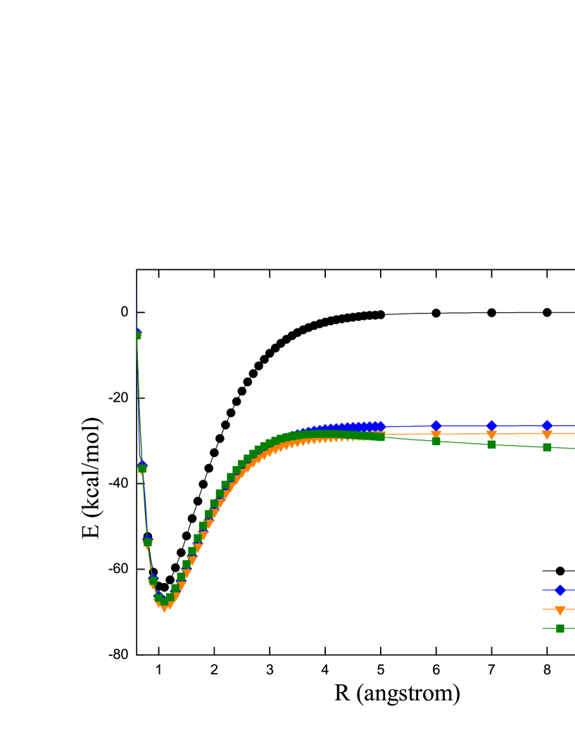
Figure 1: Dissociation curve of H2+. Zero level is set to E(H)+E(H+) for each method.

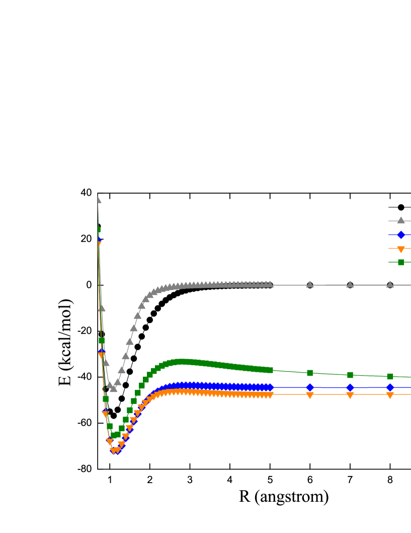
Figure 2: Dissociation curve of He2+. Zero level is set to E(He)+E(He+) for each method.

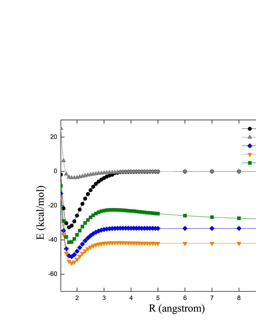
Figure 3: Dissociation curve of Ne2+. Zero level is set to E(Ne)+E(Ne+) for each method.

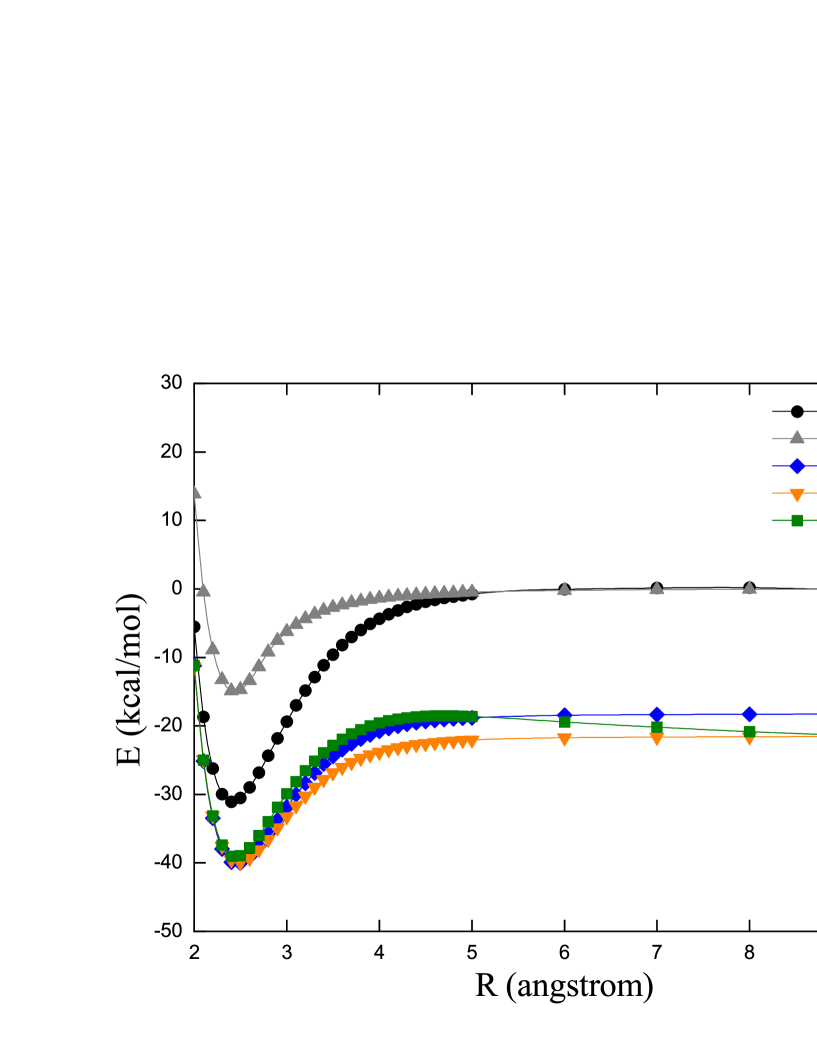
Figure 4: Dissociation curve of Ar2+. Zero level is set to E(Ar)+E(Ar+) for each method.

V.4 Frontier Orbital Energies

Let IP($N$) be the ionization potential and EA($N$) be the electron affinity of the $N$-electron system, which are defined as

$$\text{IP}(N)={E}_{N-1}-{E}_{N},$$ (39)

$$\text{EA}(N)={E}_{N}-{E}_{N+1},$$ (40)

respectively, with ${E}_{N}$ being the total energy of $N$-electron system. For the exact DFT, the vertical ionization potential of a neutral molecule is identical to the minus HOMO (highest occupied molecular orbital) energy of the neutral molecule Levy et al. (1984); Parr and Yang (1989),

$$\text{IP}(N)=-{\epsilon}_{N}(N),$$ (41)

and the vertical electron affinity of a neutral molecule is identical to the minus HOMO energy of the anion (since EA($N$) = IP($N+1$) by definition),

$$\text{EA}(N)=-{\epsilon}_{N+1}(N+1),$$ (42)

where ${\epsilon}_{M}(N)$ is the $M$-th orbital energy of $N$-electron system. The vertical electron affinity of a neutral molecule may also be approximated by the minus LUMO (lowest unoccupied molecular orbital) energy of the neutral molecule, but it is proved that there exists a difference between the vertical EA and the minus LUMO energy,

$${\Delta}_{xc}={\epsilon}_{N+1}(N+1)-{\epsilon}_{N+1}(N),$$ (43)

where the difference ${\Delta}_{xc}$ arises from the discontinuity of exchange-correlation potentials Sham and Schl$\ddot{\text{u}}$ter (1983, 1985); Perdew and Levy (1983). Recent study shows that ${\Delta}_{xc}$ is close to zero for LC hybrid functionals Tsuneda et al. (2010), so the minus LUMO energy calculated by a LC hybrid functional should be close to the vertical EA.

To evaluate the performance of the functionals on the HOMO energy of the neutral molecule, we collect a new database, IP131, which consists of experimental vertical IPs of 18 atoms and 113 molecules in the experimental geometries. The geometries and most of the reference values are collected from the NIST database NIS . Other publications Gill et al. (1992); *Brundle72; *Niessen82; *Colbourne78; *Frost72; *Bieri82; *Cvitas77; *Bieri81; *Asbrink80; *Gelius71; *Asbrink81; *Bieri80; *Niessen80 are adopted for the experimental vertical IPs of some molecules. The DFT calculations are performed with 6-311++G(3df,3pd) basis and EML(75,302) grid. As can be seen in Table 6, $\omega$M05-D gives the best results. The global hybrid M05-2X gives the worst results here, due to its incorrect long-range XC-potential behavior.

To evaluate the performance of the functionals on the vertical electron affinity, we construct another database called EA115, which consists of 18 atoms and 97 molecules. For the molecular geometries, it is a subset of IP131. Because experimental vertical EAs are not as widely available as experimental vertical IPs, the reference values of vertical EAs are obtained via the accurate CCSD(T) calculations (using Eq. (40)). The CCSD(T) correlation energies in the basis-set limit are extrapolated from calculations using the aug-cc-pVTZ and aug-cc-pVQZ basis sets Halkier et al. (1998):

$$E_{XY}^{\infty}=\frac{E_{X}^{\text{corr}}X^{3}-E_{Y}^{\text{corr}}Y^{3}}{X^{3}-Y^{3}},$$ (44)

where $X$=3 and $Y$=4 for the aug-cc-pVTZ and aug-cc-pVQZ basis, respectively. The electron affinities are evaluated in two different ways, as shown in Table 7 for the minus HOMO energy of the anion, and Table 8 for the minus LUMO energy of the neutral molecule. Clearly, the LC hybrid functionals outperform the global hybrid M05-2X. The reference values and molecular geometries of IP131 and EA115 are given in the supplementary material SI along with detailed DFT results.

Table 6: Statistical errors (in eV) for the IP131 database. Error is defined as - $\epsilon_{N}(N)$ - IP${}_{\text{vertical}}$. Experimental geometries and reference values are used for all molecules.

System	Error	$\omega$M05-D	M05-2X	$\omega$B97X-D
atoms	MSE	-1.48	-2.06	-1.64
(18)	MAE	1.48	2.06	1.64
	rms	1.74	2.16	1.98
molecules	MSE	-0.68	-1.23	-0.92
(113)	MAE	0.68	1.23	0.92
	rms	0.76	1.27	1.00
total	MSE	-0.79	-1.34	-1.02
(131)	MAE	0.79	1.34	1.02
	rms	0.96	1.43	1.18

Table 7: Statistical errors (in eV) for the EA115 database. Error is defined as - $\epsilon_{N+1}(N+1)$ - EA${}_{\text{vertical}}$. Experimental geometries and CCSD(T) reference values are used for all molecules.

System	Error	$\omega$M05-D	M05-2X	$\omega$B97X-D
atoms	MSE	-0.46	-1.21	-0.53
(18)	MAE	0.49	1.21	0.57
	rms	0.73	1.35	0.84
moelcules	MSE	-0.54	-1.18	-0.54
(97)	MAE	0.55	1.18	0.56
	rms	0.80	1.32	0.82
total	MSE	-0.53	-1.18	-0.54
(115)	MAE	0.55	1.18	0.56
	rms	0.79	1.32	0.82

Table 8: Statistical errors (in eV) of the minus LUMO energy of the neutral molecule for the EA115 database. Experimental geometries and CCSD(T) reference values are used for all molecules.

System	Error	$\omega$M05-D	M05-2X	$\omega$B97X-D
atoms	MSE	-0.27	0.57	-0.02
(18)	MAE	0.73	1.02	0.74
	rms	0.92	1.12	0.89
moelcules	MSE	-0.24	0.60	0.05
(97)	MAE	0.60	0.75	0.52
	rms	0.69	0.94	0.60
total	MSE	-0.24	0.60	0.04
(115)	MAE	0.62	0.79	0.55
	rms	0.73	0.97	0.65

V.5 Fundamental Gaps

The fundamental gap $E_{g}$ of a molecule with $N$ electrons is defined as

$$E_{g}=\text{IP}(N)-\text{EA}(N).$$ (45)

Following Eqs. (39) and (40) for the definitions of IP and EA, three self-consistent field (SCF) calculations (for the neutral molecule, cation and anion) are required to obtain the fundamental gap of a molecule. Using Eq. (41) and (42), the fundamental gap of a molecule can also be obtained by two SCF calculations (for the neutral molecule and anion).

Following Janak’s theorem Janak (1978), the fundamental gap can be approximated by the HOMO-LUMO gap Perdew and Levy (1983)

$${\Delta}_{KS}={\epsilon}_{N+1}(N)-{\epsilon}_{N}(N),$$ (46)

and we can obtain the fundamental gap of a system using only one calculation. But from Eqs. (41), (42), (43), (45), and (46), we know that there exists a difference between the fundamental gap and HOMO-LUMO gap,

$$E_{g}={\Delta}_{KS}+{\Delta}_{xc}.$$ (47)

As previously mentioned, ${\Delta}_{xc}$ has been shown to be close to zero for LC hybrid functionals Tsuneda et al. (2010), so the HOMO-LUMO gap calculated by a LC hybrid functional should be close to the fundamental gap.

To evaluate the performance of the functionals on fundamental gap, we construct another database called FG115, which shares the same molecular geometries with the EA115 database. For consistency, the reference values of fundamental gaps are also obtained via the CCSD(T) calculations described in the last subsection (using Eqs. (39), (40), and (45)).

To examine the performance of density functionals, we evaluate the fundamental gaps using three different estimates, with 6-311++G(3df,3pd) basis and EML(75,302) grid. The results are shown from Table 9 to Table 11, in order of increasing the number of SCF calculations required for each molecule. In the estimate requiring three calculations, the results are similar for the three functionals. $\omega$B97X-D gives worse results than other functionals in the estimate requiring two calculations. In the simplest estimate, the HOMO-LUMO gap, which requires only one SCF calculation for each system, $\omega$M05-D significantly outperforms the other two functionals. The reference values of FG115 and detailed HOMO-LUMO gap results by DFT methods are given in the supplementary material SI .

Table 9: Statistic errors (in eV) of HOMO-LUMO gaps for the FG115 database. The energy gap of each system is evaluated by only one SCF calculation.

System	Error	$\omega$M05-D	M05-2X	$\omega$B97X-D
atoms	MSE	-1.14	-2.56	-1.55
(18)	MAE	1.43	2.56	1.79
	rms	1.62	2.79	2.05
molecules	MSE	-0.62	-2.00	-1.15
(97)	MAE	0.73	2.00	1.15
	rms	0.93	2.13	1.34
total	MSE	-0.70	-2.08	-1.21
(115)	MAE	0.84	2.08	1.25
	rms	1.07	2.24	1.48

Table 10: Statistic errors (in eV) of fundamental gaps for the FG115 database, each evaluated by the difference of HOMO energies between the neutral molecule and anion. The energy gap of each system is evaluated by two SCF calculations.

System	Error	$\omega$M05-D	M05-2X	$\omega$B97X-D
atoms	MSE	-0.95	-0.83	-1.04
(18)	MAE	0.98	0.87	1.08
	rms	1.17	1.00	1.30
molecules	MSE	-0.31	-0.42	-0.55
(97)	MAE	0.56	0.51	0.72
	rms	0.70	0.60	0.85
total	MSE	-0.41	-0.48	-0.63
(115)	MAE	0.62	0.57	0.78
	rms	0.79	0.68	0.93

Table 11: Statistic errors (in eV) of IP-EA values for the FG115 database. The energy gap of each system is evaluated by three SCF calculations.

System	Error	$\omega$M05-D	M05-2X	$\omega$B97X-D
atoms	MSE	0.28	0.33	0.28
(18)	MAE	0.35	0.36	0.36
	rms	0.60	0.63	0.59
molecules	MSE	0.34	0.42	0.22
(97)	MAE	0.44	0.50	0.39
	rms	0.73	0.78	0.68
total	MSE	0.33	0.40	0.23
(115)	MAE	0.43	0.48	0.39
	rms	0.71	0.75	0.66

V.6 Excitation Energies

To assess the performance of density functionals on excitation energies, we perform TDDFT calculations on five small molecules Hirata and Head-Gordon (1999), which include nitrogen gas (N2), carbon monoxide (CO), water (H2O), ethylene (C2H4) and formaldehyde (CH2O), with 6-311(2+,2+)G** basis and EML(99,590) grid. The molecular geometries, experimental values of excitation energy are taken from Ref. Hirata and Head-Gordon (1999). The detail results and mean absolute errors of all excited states are listed in Table 12. The new $\omega$M05-D functional yields excellent performance, especially for the Rydberg excitations. Note that $\omega$M05-D outperforms $\omega$B97X-D in both HOMO energies and Rydberg excitations, due to the larger fraction of short-range HF exchange included in $\omega$M05-D (both functionals possess the same amount of LR-HF exchange).

Table 12: Vertical excitation energies (in eV) of several low-lying excited states of N₂, CO, water, formaldehyde and ethylene using 6-311(2+,2+)G** basis set. The geometries and experimental values are taken from Ref. Hirata and Head-Gordon (1999).

Mol.	State	Exp.	$\omega$M05-D	M05-2X	$\omega$B97X-D
	V1$\Pi$g	9.31	9.30	9.42	9.38
	V1$\Sigma$${}^{-}_{u}$	9.97	8.76	8.35	9.31
	V1$\Delta$u	10.27	10.14	10.51	9.82
N2	V3$\Sigma$${}^{+}_{u}$	7.75	7.86	8.30	7.17
	V3$\Pi$g	8.04	7.94	8.12	7.82
	V3$\Delta$u	8.88	8.74	8.35	8.23
	V3$\Sigma$${}^{-}_{u}$	9.67	8.76	9.26	9.31
	V3$\Pi$u	11.19	11.30	11.72	10.98
	V1$\Pi$	8.51	8.51	8.74	8.47
	V1$\Sigma$-	9.88	9.36	9.11	9.78
CO	V3$\Pi$	6.32	6.66	7.03	6.07
	V3$\Sigma$+	8.51	8.47	8.87	8.00
	V3$\Delta$	9.36	9.19	9.11	8.88
	V3$\Sigma$-	9.88	9.36	9.55	9.78
	R1B1	7.4	7.68	8.04	7.23
	R1A2	9.1	9.14	9.60	8.63
H2O	R1A1	9.7	9.73	10.29	9.20
	R1B1	10.0	9.72	10.32	9.17
	R1A1	10.17	10.06	10.71	9.49
	R3B1	7.2	7.27	7.66	6.89
	R1B3u	7.11	7.53	7.61	7.02
	V1B1u	7.60	7.80	8.07	7.52
	R1B1g	7.80	7.87	8.07	7.59
	R1B2g	8.01	8.15	8.19	7.66
	R1Ag	8.29	8.36	8.52	7.87
C2H4	R1B3u	8.62	8.76	8.80	8.36
	V3B1u	4.36	4.64	4.99	4.12
	R3B3u	6.98	7.43	7.48	6.92
	R3B1g	7.79	7.47	7.82	7.50
	R3B2g	7.79	8.06	8.07	7.56
	R3Ag	8.15	8.12	8.11	7.63
	V1A2	4.07	3.63	3.68	3.88
	R1B2	7.11	7.48	7.92	6.96
	R1B2	7.97	8.13	8.58	7.66
	R1A1	8.14	9.13	9.47	8.74
	R1A2	8.37	8.30	8.84	7.84
CH2O	R1B2	8.88	8.86	9.21	8.52
	V3A2	3.50	3.02	3.12	3.21
	V3A1	5.86	5.70	6.02	5.29
	R3B2	6.83	7.33	7.74	6.81
	R3B2	7.79	7.97	8.37	7.50
	R3A1	7.96	8.06	8.45	7.56
MAE	Valence		0.31	0.46	0.32
	Rydberg		0.22	0.47	0.35

Following Dreuw et al., we perform TDDFT calculations for the lowest charge-transfer (CT) excitation between ethylene and tetrafluroethylene, with a separation of $R$. Dreuw et al. have shown that the exact CT excitation energy from the HOMO of donor to the LUMO of acceptor should have the following asymptote Dreuw et al. (2003):

$$\omega_{\text{CT}}(R\rightarrow\infty)\approx-\frac{1}{R}+\text{IP}_{\text{D}}-\text{EA}_{\text{A}},$$ (48)

where $\text{IP}_{\text{D}}$ is the ionization potential of donor and $\text{EA}_{\text{A}}$ is the electron affinity of acceptor. Fig. 5 shows the trend of the excitation curves, and indicates the LC hybrid functionals obviously outperforms the global hybrid M05-2X. For the values of the excitation energies, as shown in Fig. 6, $\omega$M05-D is about 0.2 electron volt better than $\omega$B97X-D.

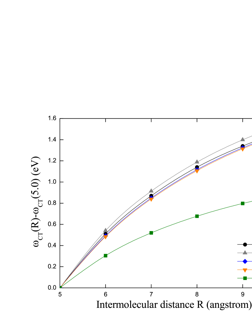
Figure 5: The lowest CT excitation of C2H4$\cdots$C2F4 dimer along the intermolecular distance $R$ (in Å). For all functionals, the excitation at 5 Å is set to zero.

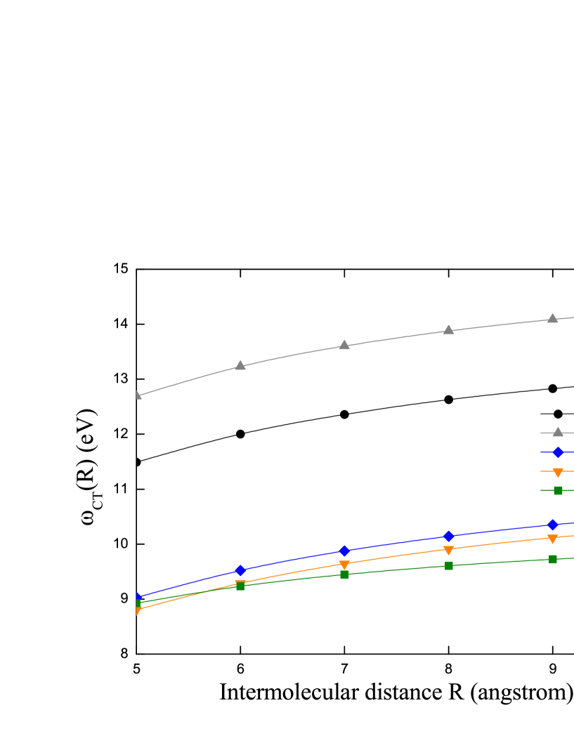
Figure 6: The lowest CT excitation of C2H4$\cdots$C2F4 dimer along the intermolecular distance $R$ (in Å).

VI CONCLUSIONS

We have developed a LC hybrid MGGA-D functional, called $\omega$M05-D, which includes 100% long-range exact exchange, a fraction ($\approx$ 37%) of short-range exact exchange, a modified M05 exchange density functional for short-range interaction, the M05 correlation density functional Zhao et al. (2005a, 2006a), and empirical atomic-pairwise dispersion corrections. For the modified short-range M05 exchange density functional, we have investigated two models. After comparisons in the training set and test sets, we decide to propose the one based on our new LC scheme $\omega$M05-D, and marked the trial one as $\omega$M05s-D. When the constraint of $\omega$ = 0 is applied, $\omega$M05-D and $\omega$M05s-D are both reduced to the existing M05 functional form Zhao et al. (2005a, 2006a) with the same empirical atomic-pairwise dispersion corrections. The constrained form ($\omega$ = 0), when re-optimized on the same training set, provides worse performance on the training set, indicating that the single extra degree of freedom corresponding to long-range exchange is of physical significance to a hybrid MGGA.

Since $\omega$M05-D is a parametrized functional, we test it against the trial simple model $\omega$M05s-D as well as two closely related functionals (M05-2X Zhao et al. (2006a) and $\omega$B97X-D Chai and Head-Gordon (2008b)) on a separate independent test set of data, which includes further atomization energies, reaction energies, noncovalent interaction energies, equilibrium geometries, energy curve for homonuclear diatomic cation dissociations, frontier orbital energies and fundamental gaps. The three databases assessing frontier orbital energies and fundamental gaps are presented for the first time. For excitation energies, we calculate valence and Rydberg excitations, as well as a charge-transfer excited state. Compared to $\omega$M05s-D, noticeable difference in transferability for atomization energies largely decides our proposed model. $\omega$M05-D consistently outperforms M05-2X (and performs comparably to $\omega$B97X-D) on the test sets, and shows smaller SIE and better asymptotic behavior relative to both the M05-2X and $\omega$B97X-D.

Supplementary material

Table 13: -$\epsilon_{N}(N)$ (in eV) of IP131 database. Most experimental reference values are collected from the NIST database, NIS while other publications Gill et al. (1992); Brundle et al. (1972); von Niessen et al. (1982); Colbourne et al. (1978); Frost et al. (1972); Bieri et al. (1982); Cvitas et al. (1977); Bieri et al. (1981); Åsbrink et al. (1980); Gelius et al. (1971); Åsbrink et al. (1981); Bieri and Åsbrink (1980); von Niessen et al. (1980) are adopted for the molecules marked.

Molecule	Reference	$\omega$M05-D	M05-2X	$\omega$B97X-D
H (Hydrogen atom)	13.60	11.10	10.44	11.04
He (Helium atom)	24.59	20.75	20.75	20.18
Li (Lithium atom)	5.39	5.06	4.19	5.22
Be (Beryllium atom) Gill et al. (1992)	9.32	8.19	7.29	8.27
B (Boron atom)	8.30	7.21	6.39	7.24
C (Carbon atom)	11.26	9.74	9.11	9.57
N (Nitrogen atom)	14.53	12.46	12.02	12.13
O (Oxygen atom)	13.62	11.80	11.51	11.48
F (Fluorine atom)	17.42	15.15	15.10	14.63
Ne (Neon atom)	21.57	18.77	18.93	18.06
Na (Sodium atom)	5.14	4.92	4.08	4.87
Mg (Magnesium atom)	7.65	7.15	6.36	7.07
Al (Aluminum atom)	5.99	5.33	4.43	5.47
Si (Silicon atom)	8.15	7.29	6.42	7.29
P (Phosphorus atom)	10.49	9.33	8.51	9.25
S (Sulfur atom)	10.36	9.33	8.65	9.30
Cl (Chlorine atom)	12.97	11.70	11.12	11.56
Ar (Argon atom)	15.76	14.17	13.68	13.93
CH3 (Methyl radical)	9.84	8.79	7.92	8.60
CH4 (Methane)	13.60	13.16	12.59	12.97
NH (Imidogen) (${}^{3}{\Sigma}^{-}$)	13.49	11.97	11.51	11.64
NH2 (Amino radical)	12.00	10.99	10.47	10.74
NH3 (Ammonia)	10.82	10.01	9.41	9.74
OH (Hydroxyl radical)	13.02	11.64	11.32	11.26
H2O (Water) Brundle et al. (1972)	12.62	11.51	11.10	11.10
HF (Hydrogen fluoride)	16.12	14.42	14.28	13.90
SiH3 (Silyl)	8.74	8.19	7.32	8.16
SiH4 (Silane)	12.30	11.86	11.18	11.80
PH3 (Phosphine)	10.59	9.79	9.03	9.76
H2S (Hydrogen sulfide)	10.50	9.57	8.84	9.47
HCl (Hydrogen sulfide) von Niessen et al. (1982)	12.77	11.64	11.02	11.45
C2H2 (Acetylene)	11.49	10.61	9.85	10.36
C2H4 (Ethylene)	10.68	10.01	9.17	9.74
C2H6 (Ethane)	11.99	11.70	11.15	11.59
HCN (Hydrogen cyanide)	13.61	12.62	11.97	12.35
CO (Carbon monoxide)	14.01	12.97	12.51	12.81
HCO (Formyl radical)	9.31	8.81	8.30	8.62
H2CO (Formaldehyde)	10.89	10.09	9.60	9.82
CH3OH (Methyl alcohol)	10.96	10.23	9.76	9.93
N2 (Nitrogen diatomic)	15.58	14.58	14.25	14.28
N2H4 (Hydrazine)	8.98	9.03	8.46	8.79
NO (Nitric oxide)	9.26	8.70	8.35	8.35
O2 (Oxygen diatomic) (${}^{3}{\Sigma}_{g}$)	12.30	11.48	11.26	11.02
H2O2 (Hydrogen peroxide)	11.70	10.77	10.42	10.36
F2 (Fluorine diatomic)	15.70	14.44	14.39	13.90
CO2 (Carbon dioxide)	13.78	12.97	12.54	12.65
P2 (Phosphorus diatomic)	10.62	9.93	9.14	9.90
S2 (Sulfur diatomic) (${}^{3}{\Sigma}_{g}$)	9.55	8.95	8.30	8.87
Cl2 (Chlorine diatomic)	11.49	10.77	10.17	10.64
NaCl (Sodium Chloride)	9.80	8.60	7.94	8.40
SiO (Silicon monoxide) Colbourne et al. (1978)	11.61	10.88	10.20	10.77
CS (Carbon monosulfide) Frost et al. (1972)	11.34	10.99	10.42	10.91
ClO (Monochlorine monoxide)	11.01	10.12	9.71	9.90
ClF (Chlorine monofluoride)	12.77	11.67	11.18	11.45
Si2H6 (Disilane)	10.53	10.15	9.41	10.12
CH3Cl (Methyl chloride)	11.29	10.61	9.98	10.42
CH3SH (Methanethiol)	9.44	8.79	8.05	8.68
SO2 (Sulfur dioxide)	12.50	11.78	11.29	11.59
BF3 (Borane, trifluoro-)	15.96	14.82	14.72	14.28
BCl3 (Borane, trichloro-)	11.64	11.18	10.58	11.02
AlCl3 (Aluminum trichloride)	12.01	11.48	10.85	11.29
CF4 (Carbon tetrafluoride)	16.20	15.23	15.15	14.69
CCl4 (Carbon tetrachloride)	11.69	11.15	10.58	10.99
OCS (Carbonyl sulfide)	11.19	10.64	9.96	10.53
CS2 (Carbon disulfide)	10.09	9.57	8.89	9.57
CF2O (Carbonic difluoride)	13.60	12.78	12.43	12.38
SiF4 (Silicon tetrafluoride)	16.40	15.37	15.26	14.85
N2O (Nitrous oxide)	12.89	12.00	11.51	11.75
NF3 (Nitrogen trifluoride)	13.60	12.62	12.35	12.32
PF3 (Phosphorus trifluoride)	12.20	10.74	10.17	10.69
O3 (Ozone)	12.73	12.35	11.91	11.97
F2O (Difluorine monoxide)	13.26	12.51	12.40	12.02
ClF3 (Chlorine trifluoride)	13.05	12.19	11.86	11.86
C2F4 (Tetrafluoroethylene)	10.69	9.93	9.41	9.71
CF3CN (Acetonitrile, trifluoro-)	14.30	13.30	12.73	13.00
CH3CCH (Propyne)	10.37	9.82	9.08	9.60
CH2CCH2 (Allene)	10.20	9.79	9.06	9.60
C3H4 (Cyclopropene)	9.86	9.33	8.60	9.11
C3H6 (Cyclopropane)	10.54	10.47	9.74	10.28
C3H8 (Propane)	11.51	11.21	10.66	11.10
CH3CCCH3 (2-Butyne)	9.79	9.19	8.46	8.98
C4H6 (Cyclobutene)	9.43	9.19	8.43	8.98
CH3CH(CH3)CH3 (Isobutane)	11.13	10.99	10.42	10.85
C6H6 (Benzene)	9.25	9.28	8.49	9.06
CH2F2 (Methane, difluoro-)	13.27	12.27	11.97	11.97
CHF3 (Methane, trifluoro-)	15.50	13.52	13.27	13.22
CH2Cl2 (Methylene chloride)	11.40	10.85	10.28	10.72
CHCl3 (Chloroform)	11.50	10.85	10.28	10.72
CH3NO2 (Methane, nitro-)	11.29	11.12	10.77	10.72
CH3SiH3 (Methyl silane)	11.60	11.23	10.50	11.12
HCOOH (Formic acid)	11.50	10.69	10.23	10.36
CH3CONH2 (Acetamide)	10.00	9.66	9.17	9.36
C2H5N (Aziridine)	9.85	9.36	8.73	9.11
C2N2 (Cyanogen)	13.51	12.78	12.19	12.54
CH3NHCH3 (Dimethylamine)	8.95	8.60	7.97	8.38
CH2CO (Ketene)	9.64	9.19	8.49	9.00
C2H4O (Ethylene oxide)	10.57	10.25	9.79	9.90
C2H2O2 (Ethanedial)	10.60	10.12	9.63	9.87
CH3CH2OH (Ethanol)	10.64	10.09	9.63	9.79
CH3OCH3 (Dimethyl ether)	10.10	9.66	9.14	9.36
C2H4S (Thiirane)	9.05	8.57	7.86	8.46
CH3SOCH3 (Dimethyl sulfoxide)	9.10	8.76	8.16	8.57
CH2CHF (Ethene, fluoro-)	10.63	9.90	9.17	9.66
CH3CH2Cl (Ethyl chloride)	11.06	10.44	9.85	10.28
CH2CHCl (Ethene, chloro-)	10.20	9.60	8.87	9.41
CH3COCl (Acetyl Chloride)	11.03	10.77	10.23	10.53
CH2ClCH2CH3 (Propane, 1-chloro-)	10.88	10.42	9.76	10.25
N(CH3)3 (Trimethylamine)	8.54	8.27	7.62	8.05
C4H4O (Furan)	8.90	8.70	7.92	8.51
C4H5N (Pyrrole)	8.23	8.13	7.32	7.92
NO2 (Nitrogen dioxide)	11.23	10.72	10.42	10.36
SF6 (Sulfur Hexafluoride) Bieri et al. (1982)	15.70	14.96	14.91	14.42
CFCl3 (Trichloromonofluoromethane)	11.76	11.23	10.66	11.07
CF3Cl (Methane, chlorotrifluoro-)	13.08	12.27	11.75	12.05
CF3Br (Bromotrifluoromethane) Cvitas et al. (1977)	12.08	11.29	10.74	11.12
HCCF (Fluoroacetylene) Bieri et al. (1981)	11.50	10.53	9.85	10.28
HCCCN (Cyanoacetylene) Åsbrink et al. (1980)	11.75	11.07	10.42	10.85
C4N2 (2-Butynedinitrile) Bieri and Åsbrink (1980)	11.84	11.56	10.96	11.34
C2N2 (Cyanogen)	13.51	12.78	12.19	12.54
C3O2 (Carbon suboxide) Gelius et al. (1971)	10.80	10.39	9.82	10.23
FCN (Cyanogen fluoride) Åsbrink et al. (1981)	13.65	12.46	11.89	12.16
C4H2 (Diacetylene)	10.30	9.71	9.00	9.52
H2CS (Thioformaldehyde)	9.38	8.73	8.02	8.62
CHONH2 (Formamide) Åsbrink et al. (1981)	10.40	9.90	9.44	9.57
CH2CHCHO (Acrolein) von Niessen et al. (1980)	10.10	9.90	9.38	9.57
CH2CCl2 (Ethene, 1,1-dichloro-)	10.00	9.57	8.87	9.41
C2HF3 (Trifluoroethylene) Bieri et al. (1981)	10.62	9.74	9.14	9.52
CH2CF2 (Ethene, 1,1-difluoro-) Bieri et al. (1981)	10.70	10.01	9.33	9.76
CH3F (Methyl fluoride)	13.04	12.21	11.86	11.91
CF2Cl2 (Difluorodichloromethane)	12.24	11.61	11.07	11.45
SiF2 (Silicon difluoride)	11.08	10.25	9.52	10.23
MSE		-0.79	-1.34	-1.02
MAE		0.79	1.34	1.02
rms		0.96	1.43	1.18

Table 14: -$\epsilon_{N+1}(N+1)$ and -$\epsilon_{N+1}(N)$ (in eV) of EA115 database. Reference values are calculated by the CCSD(T) theory.

	reference	$\omega$M05-D		M05-2X		$\omega$B97X-D
molecule		-$\epsilon_{N+1}(N+1)$	-$\epsilon_{N+1}(N)$	-$\epsilon_{N+1}(N+1)$	-$\epsilon_{N+1}(N)$	-$\epsilon_{N+1}(N+1)$	-$\epsilon_{N+1}(N)$
H (Hydrogen atom)	0.75	0.84	-0.52	-0.08	-0.53	0.84	-0.53
He (Helium atom)	-2.63	-4.35	-4.76	-5.17	-3.89	-4.27	-4.30
Li (Lithium atom)	0.62	0.68	-0.44	0.00	0.14	0.71	-0.19
Be (Beryllium atom)	-0.36	-0.46	-0.52	-1.20	0.35	-0.41	-0.30
B (Boron atom)	0.25	0.19	0.38	-0.65	1.28	0.16	0.57
C (Carbon atom)	1.25	0.87	1.69	0.08	2.42	0.73	1.99
N (Nitrogen atom)	-0.22	-0.60	0.49	-1.39	1.55	-0.63	0.52
O (Oxygen atom)	1.45	0.76	2.18	0.16	2.96	0.54	2.48
F (Fluorine atom)	3.44	2.28	4.30	1.90	4.81	1.93	4.90
Ne (Neon atom)	-5.31	-7.18	-7.07	-8.16	-5.82	-7.53	-6.83
Na (Sodium atom)	0.54	0.68	-0.49	0.05	-0.03	0.68	-0.24
Mg (Magnesium atom)	-0.23	-0.41	-0.65	-0.98	0.11	-0.30	-0.38
Al (Aluminum atom)	0.45	0.27	0.22	-0.54	1.12	0.33	0.35
Si (Silicon atom)	1.42	1.09	1.41	0.22	2.31	1.06	1.55
P (Phosphorus atom)	0.74	0.57	0.98	-0.24	2.20	0.63	1.20
S (Sulfur atom)	2.10	1.77	2.53	1.01	3.64	1.71	2.77
Cl (Chlorine atom)	3.69	3.05	4.27	2.34	5.22	2.91	4.57
Ar (Argon atom)	-2.81	-3.18	-3.78	-4.03	-2.53	-3.48	-3.40
CH3 (Methyl radical)	-0.07	-0.08	-0.08	-0.92	1.09	-0.16	-0.05
CH4 (Methane)	-0.62	-1.01	-1.52	-1.58	-0.92	-0.92	-1.17
NH (Imidogen)	0.33	-0.03	0.65	-0.79	1.66	-0.14	0.84
NH2 (Amino radical)	0.74	0.44	0.90	-0.33	1.85	0.27	1.12
NH3 (Ammonia)	-0.56	-0.98	-1.52	-1.63	-0.76	-0.90	-1.12
OH (Hydroxyl radical)	1.83	1.22	2.15	0.63	2.91	0.95	2.53
H2O (Water)	-0.56	-1.03	-1.50	-1.80	-0.68	-0.95	-1.09
HF (Hydrogen fluoride)	-0.63	-1.14	-1.47	-1.85	-0.73	-1.01	-1.12
SiH3 (Silyl)	0.93	0.79	1.14	-0.03	2.53	0.82	1.31
SiH4 (Silane)	-1.11	-1.09	-1.69	-1.60	-0.95	-1.06	-1.28
PH3 (Phosphine)	-1.21	-0.90	-1.50	-1.44	-0.71	-0.90	-1.09
SH2 (Hydrogen sulfide)	-0.49	-1.85	-1.41	-2.39	-0.63	-1.69	-1.03
HCl (Hydrogen chloride)	-0.52	-0.92	-1.36	-1.63	-0.54	-0.84	-0.98
C2H2 (Acetylene)	-1.90	-2.50	-1.52	-3.24	-1.09	-2.56	-1.22
C2H4 (Ethylene)	-1.86	-2.07	-1.74	-2.86	-0.92	-2.12	-1.33
C2H6 (Ethane)	-0.62	-1.03	-1.55	-1.55	-0.90	-0.95	-1.17
HCN (Hydrogen cyanide)	-0.48	-2.07	-1.41	-2.83	-0.92	-2.01	-1.09
CO (Carbon monoxide)	-1.50	-1.90	-1.33	-2.67	-0.46	-1.93	-1.09
HCO (Formyl radical)	0.02	-0.27	0.44	-1.01	1.39	-0.33	0.57
CH2O (Formaldehyde)	-0.55	-1.31	-0.63	-2.09	0.19	-1.41	-0.46
CH3OH (Methyl alcohol)	-0.55	-0.95	-1.44	-1.50	-0.79	-0.84	-1.09
N2 (Nitrogen diatomic)	-2.24	-2.80	-1.55	-3.56	-0.71	-2.88	-1.28
N2H4 (Hydrazine)	-0.45	-1.52	-1.41	-1.99	-0.57	-1.39	-1.01
NO (Nitric oxide)	-0.42	-0.92	0.60	-1.52	1.44	-1.12	0.87
O2 (Oxygen diatomic)	-0.08	-0.87	0.79	-1.36	1.60	-1.09	1.12
H2O2 (Hydrogen peroxide)	-0.92	-1.47	-1.63	-2.04	-0.82	-1.33	-1.25
F2 (Fluorine diatomic)	0.42	-0.38	1.69	-0.57	2.42	-0.73	2.15
CO2 (Carbon dioxide)	-0.65	-4.49	-1.69	-5.11	-0.73	-4.68	-1.31
P2 (Phosphorus diatomic)	0.48	0.33	0.73	-0.46	1.71	0.35	0.95
S2 (Sulfur diatomic)	1.53	1.12	1.69	0.44	2.72	1.12	1.93
Cl2 (Chlorine diatomic)	0.75	0.38	1.06	-0.33	1.99	0.27	1.33
NaCl (Sodium Chloride)	0.65	0.52	0.16	-0.16	0.79	0.65	0.46
SiO (Silicon monoxide)	0.03	-0.33	0.11	-1.12	1.09	-0.24	0.33
CS (Carbon monosulfide)	-0.09	-0.30	0.33	-1.03	1.25	-0.33	0.54
ClO (Monochlorine monoxide)	2.19	1.60	2.58	1.06	3.37	1.41	2.77
ClF (Chlorine monofluoride)	0.44	-0.14	0.92	-0.79	1.85	-0.22	1.28
Si2H6 (Disilane)	-0.69	-1.22	-1.58	-1.69	-0.76	-1.17	-1.20
CH3Cl (Methyl chloride)	-0.51	-0.84	-1.39	-1.47	-0.68	-0.76	-1.01
CH3SH (Methanethiol)	-0.50	-0.87	-1.41	-1.44	-0.63	-0.79	-1.03
SO2 (Sulfur dioxide)	0.81	0.41	1.41	-0.19	2.42	0.30	1.66
BF3 (Borane, trifluoro-)	-1.04	-1.25	-1.71	-1.88	-0.82	-1.17	-1.31
BCl3 (Borane, trichloro-)	-0.17	-1.01	-0.16	-1.52	0.76	-0.98	-0.03
AlCl3 (Aluminum trichloride)	0.06	-0.08	-0.35	-0.79	0.73	-0.11	-0.19
CF4 (Carbon tetrafluoride)	-1.33	-1.96	-2.48	-2.53	-1.52	-1.82	-2.04
CCl4 Carbon tetrachloride)	-0.46	-0.35	-0.41	-1.01	0.57	-0.35	-0.14
OCS (Carbonyl sulfide)	-0.74	-1.58	-1.03	-2.26	-0.08	-1.58	-0.82
CS2 (Carbon disulfide)	0.01	-0.11	0.16	-0.79	1.12	-0.11	0.35
CF2O (Carbonic difluoride)	-2.37	-2.50	-1.55	-3.40	-0.65	-2.42	-1.36
SiF4 (Silicon tetrafluoride)	-0.81	-1.25	-1.66	-1.88	-0.63	-1.22	-1.22
N2O (Nitrous oxide)	-2.01	-2.58	-1.58	-3.26	-0.65	-2.75	-1.36
NF3 (Nitrogen trifluoride)	-2.06	-2.88	-2.67	-3.64	-1.82	-2.86	-2.37
PF3 (Phosphorus trifluoride)	-1.23	-1.58	-1.88	-2.12	-0.98	-1.50	-1.55
O3 (Ozone)	1.93	1.90	3.24	1.58	4.22	1.55	3.48
F2O (Difluorine monoxide)	-0.31	-1.01	0.44	-1.36	1.22	-1.17	0.82
ClF3 (Chlorine trifluoride)	1.20	0.63	1.60	0.14	2.56	0.52	1.90
C2F4 (Tetrafluoroethylene)	-1.65	-2.42	-2.07	-2.94	-1.03	-2.34	-1.66
CH3CCH (Propyne)	-1.13	-1.77	-1.41	-2.23	-0.82	-1.60	-1.06
CH2CCH2 (Allene)	-0.56	-1.55	-1.60	-2.04	-0.92	-1.41	-1.22
C3H4 (Cyclopropene)	-1.82	-2.01	-1.66	-2.80	-0.92	-2.07	-1.31
C3H6 (Cyclopropane)	-0.65	-1.17	-1.71	-1.63	-1.03	-1.09	-1.33
CH2F2 (Methane, difluoro-)	-0.58	-1.06	-1.52	-1.63	-0.95	-0.90	-1.20
CF3H (Methane, trifluoro-)	-0.60	-1.17	-1.58	-1.85	-1.01	-1.01	-1.25
CH2Cl2 (Methylene chloride)	-0.49	-0.82	-1.31	-1.50	-0.49	-0.73	-0.98
CHCl3 (Chloroform)	-0.83	-0.79	-1.01	-1.52	-0.05	-0.73	-0.76
CH3NO2 (Methane, nitro-)	-0.37	-0.49	0.05	-1.06	0.98	-0.65	0.27
CH3SiH3 (Methyl silane)	-0.53	-0.92	-1.47	-1.47	-0.73	-0.84	-1.09
HCOOH (Formic acid)	-0.57	-2.15	-1.63	-2.88	-0.87	-2.18	-1.25
CH3CONH2 (Acetamide)	-0.31	-1.60	-1.22	-2.09	-0.49	-1.44	-0.84
C2N2 (Cyanogen)	-0.19	-0.33	0.52	-1.03	1.47	-0.38	0.68
CH2CO (Ketene)	-0.51	-1.41	-1.03	-1.96	-0.16	-1.28	-0.87
C2H4O (Ethylene oxide)	-0.86	-1.03	-1.60	-1.55	-0.95	-0.95	-1.22
C2H2O2 (Ethanedial)	0.69	0.63	1.28	-0.11	2.18	0.49	1.41
CH3CH2OH (Ethanol)	-0.53	-0.92	-1.44	-1.47	-0.76	-0.82	-1.09
CH3OCH3 (Dimethyl ether)	-0.58	-1.01	-1.52	-1.47	-0.84	-0.90	-1.14
C2H4S (Thiirane)	-0.78	-1.25	-1.60	-1.69	-0.87	-1.14	-1.20
CH2CHF (Ethene, fluoro-)	-0.88	-2.18	-1.66	-2.91	-1.01	-2.23	-1.28
CH3CH2Cl (Ethyl chloride)	-0.51	-0.90	-1.47	-1.44	-0.73	-0.79	-1.09
CH2CHCl (Ethene, chloro-)	-1.11	-1.60	-1.41	-2.39	-0.52	-1.66	-1.20
CH3CClO (Acetyl Chloride)	-0.85	-1.12	-0.79	-1.80	0.11	-1.14	-0.65
NO2 (Nitrogen dioxide)	1.44	0.90	1.99	0.38	3.02	0.76	2.18
CFCl3 (Trichloromonofluoromethane)	-0.68	-0.76	-0.65	-1.39	0.33	-0.73	-0.41
CF3Cl (Methane, chlorotrifluoro-)	-1.06	-1.63	-1.82	-2.28	-0.84	-1.55	-1.52
HCCF (Fluoroacetylene)	-0.55	-0.95	-1.39	-1.47	-0.82	-0.82	-1.09
HCCCN (Cyanoacetylene)	-0.36	-0.76	-0.19	-1.52	0.71	-0.79	-0.08
C4N2 (2-Butynedinitrile)	0.68	0.76	1.25	0.05	2.20	0.71	1.36
C2N2 (Cyanogen)	-0.19	-0.33	0.52	-1.03	1.47	-0.38	0.68
C3O2 (Carbon suboxide)	-0.74	-1.01	-0.19	-1.66	0.76	-1.12	-0.05
FCN (Cyanogen fluoride)	-0.66	-4.08	-1.31	-4.81	-0.33	-4.22	-0.95
C4N2 (Diacetylene)	-0.64	-1.28	-0.92	-2.01	-0.03	-1.28	-0.82
H2CS (Thioformaldehyde)	0.28	0.11	0.68	-0.68	1.55	0.05	0.82
CHONH2 (Formamide)	-0.35	-2.48	-1.33	-3.21	-0.63	-2.45	-0.95
CH2CCl2 (Ethene, 1,1-dichloro-)	-1.07	-1.01	-1.12	-1.58	-0.19	-0.90	-0.98
C2HF3 (Trifluoroethylene)	-0.54	-1.14	-1.60	-1.74	-0.92	-0.98	-1.25
CH2CF2 (Ethene, 1,1-difluoro-)	-1.03	-2.26	-1.66	-2.96	-0.95	-2.31	-1.28
CH3F (Methyl fluoride)	-0.58	-0.98	-1.50	-1.55	-0.90	-0.87	-1.14
CF2Cl2 (Difluorodichloromethane)	-0.90	-1.31	-1.20	-1.90	-0.22	-1.28	-0.92
SiF2 (Silicon difluoride)	0.10	-0.27	0.22	-1.06	1.20	-0.19	0.44
MSE		-0.53	-0.24	-1.18	0.60	-0.54	0.04
MAE		0.55	0.62	1.18	0.79	0.56	0.55
rms		0.79	0.73	1.32	0.97	0.82	0.65

Table 15: Reference values of FG115 database calculated by the CCSD(T) theory, compared with HOMO-LUMO gap results by DFT methods.

Molecule	Reference	$\omega$M05-D	M05-2X	$\omega$B97X-D
H (Hydrogen atom)	12.86	11.62	10.98	11.57
He (Helium atom)	27.23	25.57	24.70	24.56
Li (Lithium atom)	4.22	5.49	4.05	5.41
Be (Beryllium atom)	9.66	8.70	6.94	8.57
B (Boron atom)	7.99	6.83	5.11	6.66
C (Carbon atom)	9.97	8.05	6.69	7.59
N (Nitrogen atom)	14.74	11.97	10.47	11.61
O (Oxygen atom)	12.14	9.63	8.54	9.00
F (Fluorine atom)	13.98	10.88	10.28	9.74
Ne (Neon atom)	26.91	25.84	24.75	24.89
Na (Sodium atom)	4.14	5.41	4.11	5.11
Mg (Magnesium atom)	7.76	7.81	6.26	7.45
Al (Aluminum atom)	5.53	5.11	3.32	5.11
Si (Silicon atom)	6.73	5.88	4.11	5.74
P (Phosphorus atom)	9.78	8.35	6.31	8.05
S (Sulfur atom)	8.23	6.80	5.00	6.53
Cl (Chlorine atom)	9.30	7.43	5.90	6.99
Ar (Argon atom)	18.65	17.95	16.21	17.33
CH3 (Methyl radical)	9.86	8.87	6.83	8.54
CH4 (Methane)	15.06	14.69	13.52	14.14
NH (Imidogen) (${}^{3}{\Sigma}^{-}$)	13.17	11.32	9.85	10.80
NH2 (Amino radical)	11.34	10.09	8.62	9.63
NH3 (Ammonia)	11.54	11.53	10.17	10.85
OH (Hydroxyl radical)	11.27	9.49	8.40	8.73
H2O (Water)	13.35	13.00	11.78	12.19
HF (Hydrogen fluoride)	16.91	15.88	15.01	15.01
SiH3 (Silyl)	7.95	7.04	4.79	6.85
SiH4 (Silane)	14.03	13.55	12.13	13.08
PH3 (Phosphine)	11.82	11.29	9.74	10.85
H2S (Hydrogen sulfide)	11.00	10.99	9.47	10.50
HCl (Hydrogen chloride)	13.36	13.00	11.56	12.43
C2H2 (Acetylene)	13.43	12.13	10.93	11.59
C2H4 (Ethylene)	12.57	11.75	10.09	11.07
C2H6 (Ethane)	13.41	13.25	12.05	12.76
HCN (Hydrogen cyanide)	14.31	14.04	12.89	13.44
CO (Carbon monoxide)	15.57	14.31	12.97	13.90
HCO (Formyl radical)	9.56	8.38	6.91	8.05
CH2O (Formaldehyde)	11.56	10.72	9.41	10.28
CH3OH (Methyl alcohol)	11.67	11.67	10.55	11.02
N2 (Nitrogen diatomic)	17.88	16.13	14.96	15.56
N2H4 (Hydrazine)	10.29	10.44	9.03	9.79
NO (Nitric oxide)	10.11	8.11	6.91	7.48
O2 (Oxygen diatomic) (${}^{3}{\Sigma}_{g}$)	12.52	10.69	9.66	9.90
H2O2 (Hydrogen peroxide)	12.65	12.40	11.23	11.61
F2 (Fluorine diatomic)	15.53	12.76	11.97	11.75
CO2 (Carbon dioxide)	14.58	14.66	13.27	13.95
P2 (Phosphorus diatomic)	10.19	9.19	7.43	8.95
S2 (Sulfur diatomic) (${}^{3}{\Sigma}_{g}$)	7.96	7.26	5.58	6.94
Cl2 (Chlorine diatomic)	10.93	9.71	8.19	9.30
NaCl (Sodium Chloride)	8.64	8.43	7.15	7.94
SiO (Silicon monoxide)	11.60	10.77	9.11	10.44
CS (Carbon monosulfide)	11.58	10.66	9.17	10.36
ClO (Monochlorine monoxide)	8.85	7.53	6.34	7.13
ClF (Chlorine monofluoride)	12.43	10.74	9.33	10.17
Si2H6 (Disilane)	11.33	11.72	10.17	11.32
CH3Cl (Methyl chloride)	12.01	12.00	10.66	11.42
CH3SH (Methanethiol)	10.01	10.20	8.68	9.71
SO2 (Sulfur dioxide)	11.74	10.36	8.87	9.93
BF3 (Borane, trifluoro-)	17.22	16.54	15.53	15.59
BCl3 (Borane, trichloro-)	12.07	11.34	9.82	11.04
AlCl3 (Aluminum trichloride)	12.13	11.83	10.12	11.48
CF4 (Carbon tetrafluoride)	17.85	17.71	16.67	16.73
CCl4 (Carbon tetrachloride)	11.97	11.56	10.01	11.12
OCS (Carbonyl sulfide)	12.13	11.67	10.04	11.34
CS2 (Carbon disulfide)	10.19	9.41	7.78	9.22
CF2O (Carbonic difluoride)	16.08	14.33	13.08	13.74
SiF4 (Silicon tetrafluoride)	16.95	17.03	15.88	16.08
N2O (Nitrous oxide)	15.01	13.57	12.16	13.11
NF3 (Nitrogen trifluoride)	15.76	15.29	14.17	14.69
PF3 (Phosphorus trifluoride)	13.00	12.62	11.15	12.24
O3 (Ozone)	11.06	9.11	7.70	8.49
F2O (Difluorine monoxide)	13.82	12.08	11.18	11.21
ClF3 (Chlorine trifluoride)	11.79	10.58	9.30	9.96
C2F4 (Tetrafluoroethylene)	12.45	12.00	10.44	11.37
CH3CCH (Propyne)	11.69	11.23	9.90	10.66
CH2CCH2 (Allene)	10.83	11.40	9.98	10.83
C3H4 (Cyclopropene)	11.87	10.99	9.52	10.42
C3H6 (Cyclopropane)	11.64	12.19	10.77	11.61
CH2F2 (Methane, difluoro-)	14.15	13.79	12.92	13.16
CF3H (Methane, trifluoro-)	15.44	15.10	14.28	14.47
CH2Cl2 (Methylene chloride)	12.18	12.16	10.77	11.70
CHCl3 (Chloroform)	12.38	11.86	10.34	11.48
CH3NO2 (Methane, nitro-)	11.94	11.07	9.79	10.44
CH3SiH3 (Methyl silane)	12.35	12.70	11.23	12.21
HCOOH (Formic acid)	11.98	12.32	11.10	11.61
CH3CONH2 (Acetamide)	10.05	10.88	9.66	10.20
C2N2 (Cyanogen)	13.90	12.27	10.72	11.86
CH2CO (Ketene)	10.32	10.23	8.65	9.87
C2H4O (Ethylene oxide)	11.68	11.86	10.74	11.12
C2H2O2 (Ethanedial)	10.04	8.84	7.45	8.46
CH3CH2OH (Ethanol)	11.38	11.53	10.39	10.88
CH3OCH3 (Dimethyl ether)	10.79	11.18	9.98	10.50
C2H4S (Thiirane)	9.93	10.17	8.73	9.66
CH2CHF (Ethene, fluoro-)	11.55	11.56	10.17	10.93
CH3CH2Cl (Ethyl chloride)	11.74	11.91	10.58	11.37
CH2CHCl (Ethene, chloro-)	11.35	11.02	9.38	10.61
CH3COCl (Acetyl Chloride)	11.97	11.56	10.12	11.18
NO2 (Nitrogen dioxide)	9.79	8.73	7.40	8.19
CFCl3 (Trichloromonofluoromethane)	12.61	11.89	10.34	11.48
CF3Cl (Methane, chlorotrifluoro-)	14.27	14.09	12.59	13.57
HCCF (Fluoroacetylene)	12.04	11.91	10.66	11.37
HCCCN (Cyanoacetylene)	12.20	11.26	9.71	10.93
C4N2 (2-Butynedinitrile)	11.52	10.31	8.76	9.98
C2N2 (Cyanogen)	13.90	12.27	10.72	11.86
C3O2 (Carbon suboxide)	11.64	10.58	9.06	10.28
FCN (Cyanogen fluoride)	14.33	13.76	12.21	13.11
C4H2 (Diacetylene)	11.00	10.64	9.03	10.34
H2CS (Thioformaldehyde)	9.18	8.05	6.47	7.81
CHONH2 (Formamide)	10.81	11.23	10.06	10.53
CH2CCl2 (Ethene, 1,1-dichloro-)	11.17	10.69	9.06	10.39
C2HF3 (Trifluoroethylene)	11.11	11.34	10.06	10.77
CH2CF2 (Ethene, 1,1-difluoro-)	11.81	11.67	10.28	11.04
CH3F (Methyl fluoride)	14.09	13.71	12.76	13.06
CF2Cl2 (Difluorodichloromethane)	13.33	12.81	11.29	12.38
SiF2 (Silicon difluoride)	11.04	10.04	8.32	9.79
MSE		-0.70	-2.08	-1.21
MAE		0.84	2.08	1.25
rms		1.07	2.24	1.48

Table 16: Experimental molecular geometries (in angstrom) for IP131, EA115 and FG115 databases collected from the NIST database NIS . The integers following the molecule are in order the spin multiplicities of neutral species, cation and anion. The molecules with only the spin multiplicity of the neutral species shown are in neither EA115 nor FG115 database. The spin multiplicities of neutral species are experimental values specified in the NIST database NIS . Each spin multiplicity of cations and anions is decided by CCSD(T)/aug-cc-pVTZ calculations, and corresponds to the lowest energy in between various spin multiplicities.

$\ce{H}$ (Hydrogen atom)   2   Null   1
H
$\ce{He}$ (Helium atom)   1   2   2
He
$\ce{Li}$ (Lithium atom)   2   1   1
Li
$\ce{Be}$ (Beryllium atom)   1   2   2
Be
$\ce{B}$ (Boron atom)   2   1   3
B
$\ce{C}$ (Carbon atom)   3   2   4
C
$\ce{N}$ (Nitrogen atom)   4   3   3
N
$\ce{O}$ (Oxygen atom)   3   4   2
O
$\ce{F}$ (Fluorine atom)   2   3   1
F
$\ce{Ne}$ (Neon atom)   1   2   2
Ne
$\ce{Na}$ (Sodium atom)   2   1   1
Na
$\ce{Mg}$ (Magnesium atom)   1   2   2
Mg
$\ce{Al}$ (Aluminum atom)   2   1   3
Al
$\ce{Si}$ (Silicon atom)   3   2   4
Si
$\ce{P}$ (Phosphorus atom)   4   3   3
P
$\ce{S}$ (Sulfur atom)   3   4   2
S
$\ce{Cl}$ (Chlorine atom)   2   3   1
Cl
$\ce{Ar}$ (Argon atom)   1   2   2
Ar
$\ce{CH3}$ (Methyl radical)   2   1   1
C1	0.0000	0.0000	0.0000
H2	1.0790	0.0000	0.0000
H3	-0.5395	-0.9344	0.0000
H4	-0.5395	0.9344	0.0000
$\ce{CH4}$ (Methane)   1   2   2
C1	0.0000	0.0000	0.0000
H2	0.6276	0.6276	0.6276
H3	0.6276	-0.6276	-0.6276
H4	-0.6276	0.6276	-0.6276
H5	-0.6276	-0.6276	0.6276
$\ce{NH}$ (Imidogen) (${}^{3}{\Sigma}^{-}$)   3   2   2
N1	0.0000	0.0000	0.0000
H2	0.0000	0.0000	1.0362
$\ce{NH2}$ (Amino radical)   2   3   1
N1	0.0000	0.0000	0.0000
H2	0.0000	0.8036	0.6347
H3	0.0000	-0.8036	0.6347
$\ce{NH3}$ (Ammonia)   1   2   2
N1	0.0000	0.0000	0.0000
H2	0.0000	-0.9377	-0.3816
H3	0.8121	0.4689	-0.3816
H4	-0.8121	0.4689	-0.3816
$\ce{OH}$ (Hydroxyl radical)   2   3   1
O1	0.0000	0.0000	0.0000
H2	0.0000	0.0000	0.9697
$\ce{H2O}$ (Water)   1   2   2
O1	0.0000	0.0000	0.1173
H2	0.0000	0.7572	-0.4692
H3	0.0000	-0.7572	-0.4692
$\ce{HF}$ (Hydrogen fluoride)   1   2   2
F1	0.0000	0.0000	0.0000
H2	0.0000	0.0000	0.9168
$\ce{SiH3}$ (Silyl)   2   1   1
Si1	0.0000	0.0000	0.0819
H2	0.0000	1.3928	-0.3820
H3	1.2062	-0.6964	-0.3820
H4	-1.2062	-0.6964	-0.3820
$\ce{SiH4}$ (Silane)   1   2   2
Si1	0.0000	0.0000	0.0000
H2	0.8544	0.8544	0.8544
H3	-0.8544	-0.8544	0.8544
H4	-0.8544	0.8544	-0.8544
H5	0.8544	-0.8544	-0.8544
$\ce{PH3}$ (Phosphine)   1   2   2
P1	0.0000	0.0000	0.0000
H2	0.0000	-1.1932	-0.7717
H3	1.0333	0.5966	-0.7717
H4	-1.0333	0.5966	-0.7717
$\ce{H2S}$ (Hydrogen sulfide)   1   2   2
S1	0.0000	0.0000	0.0000
H2	0.0000	0.9569	0.9208
H3	0.0000	-0.9569	0.9208
$\ce{HCl}$ (Hydrogen chloride)   1   2   2
Cl1	0.0000	0.0000	0.0000
H2	0.0000	0.0000	1.2746
$\ce{C2H2}$ (Acetylene)   1   2   2
C1	0.0000	0.0000	0.6013
C2	0.0000	0.0000	-0.6013
H3	0.0000	0.0000	1.6644
H4	0.0000	0.0000	-1.6644
$\ce{C2H4}$ (Ethylene)   1   2   2
C1	0.0000	0.0000	0.6695
C2	0.0000	0.0000	-0.6695
H3	0.0000	0.9289	1.2321
H4	0.0000	-0.9289	1.2321
H5	0.0000	0.9289	-1.2321
H6	0.0000	-0.9289	-1.2321
$\ce{C2H6}$ (Ethane)   1   2   2
C1	0.0000	0.0000	0.7680
C2	0.0000	0.0000	-0.7680
H3	-1.0192	0.0000	1.1573
H4	0.5096	0.8826	1.1573
H5	0.5096	-0.8826	1.1573
H6	1.0192	0.0000	-1.1573
H7	-0.5096	-0.8826	-1.1573
H8	-0.5096	0.8826	-1.1573
$\ce{HCN}$ (Hydrogen cyanide)   1   2   2
C1	0.0000	0.0000	0.0000
H2	0.0000	0.0000	1.0640
N3	0.0000	0.0000	-1.1560
$\ce{CO}$ (Carbon monoxide)   1   2   2
C1	0.0000	0.0000	0.0000
O2	0.0000	0.0000	1.1283
$\ce{HCO}$ (Formyl radical)   2   1   1
C1	0.0000	0.0000	0.0000
H2	1.0800	0.0000	0.0000
O3	-0.5899	1.0427	0.0000
$\ce{H2CO}$ (Formaldehyde)   1   2   2
O1	0.0000	0.0000	1.2050
C2	0.0000	0.0000	0.0000
H3	0.0000	0.9429	-0.5876
H4	0.0000	-0.9429	-0.5876
$\ce{CH3OH}$ (Methyl alcohol)   1   2   2
C1	-0.0503	0.6685	0.0000
O2	-0.0503	-0.7585	0.0000
H3	-1.0807	1.0417	0.0000
H4	0.4650	1.0417	0.8924
H5	0.4650	1.0417	-0.8924
H6	0.8544	-1.0677	0.0000
$\ce{N2}$ (Nitrogen diatomic)   1   2   2
N1	0.0000	0.0000	0.5488
N2	0.0000	0.0000	-0.5488
$\ce{N2H4}$ (Hydrazine)   1   2   2
N1	0.0000	0.7230	-0.1123
N2	0.0000	-0.7230	-0.1123
H3	-0.4470	1.0031	0.7562
H4	0.4470	-1.0031	0.7562
H5	0.9663	1.0031	0.0301
H6	-0.9663	-1.0031	0.0301
$\ce{NO}$ (Nitric oxide)   2   1   3
O1	0.0000	0.0000	0.0000
N2	0.0000	0.0000	1.1508
$\ce{O2}$ (Oxygen diatomic) (${}^{3}{\Sigma}_{g}$)   3   2   2
O1	0.0000	0.0000	0.0000
O2	0.0000	0.0000	1.2075
$\ce{H2O2}$ (Hydrogen peroxide)   1   2   2
O1	0.0000	0.7375	-0.0528
O2	0.0000	-0.7375	-0.0528
H3	0.8190	0.8170	0.4220
H4	-0.8190	-0.8170	0.4220
$\ce{F2}$ (Fluorine diatomic)   1   2   2
F1	0.0000	0.0000	0.0000
F2	0.0000	0.0000	1.4119
$\ce{CO2}$ (Carbon dioxide)   1   2   2
C1	0.0000	0.0000	0.0000
O2	0.0000	0.0000	1.1621
O3	0.0000	0.0000	-1.1621
$\ce{P2}$ (Phosphorus diatomic)   1   2   2
P1	0.0000	0.0000	0.0000
P2	0.0000	0.0000	1.8934
$\ce{S2}$ (Sulfur diatomic) (${}^{3}{\Sigma}_{g}$)   3   2   2
S1	0.0000	0.0000	0.0000
S2	0.0000	0.0000	1.8892
$\ce{Cl2}$ (Chlorine diatomic)   1   2   2
Cl1	0.0000	0.0000	0.0000
Cl2	0.0000	0.0000	1.9879
$\ce{NaCl}$ (Sodium Chloride)   1   2   2
Na1	0.0000	0.0000	0.0000
Cl2	0.0000	0.0000	2.3608
$\ce{SiO}$ (Silicon monoxide)   1   2   2
Si1	0.0000	0.0000	0.0000
O2	0.0000	0.0000	1.5097
$\ce{CS}$ (Carbon monosulfide)   1   2   2
C1	0.0000	0.0000	0.0000
S2	0.0000	0.0000	1.5349
$\ce{ClO}$ (Monochlorine monoxide)   2   3   1
O1	0.0000	0.0000	0.0000
Cl2	0.0000	0.0000	1.5696
$\ce{ClF}$ (Chlorine monofluoride)   1   2   2
F1	0.0000	0.0000	0.0000
Cl2	0.0000	0.0000	1.6283
$\ce{Si2H6}$ (Disilane)   1   2   2
Si1	0.0000	0.0000	1.1600
Si2	0.0000	0.0000	-1.1600
H3	0.0000	1.3865	1.6483
H4	-1.2008	-0.6933	1.6483
H5	1.2008	-0.6933	1.6483
H6	0.0000	-1.3865	-1.6483
H7	-1.2008	0.6933	-1.6483
H8	1.2008	0.6933	-1.6483
$\ce{CH3Cl}$ (Methyl chloride)   1   2   2
C1	0.0000	0.0000	0.0000
Cl2	0.0000	0.0000	1.7810
H3	1.0424	0.0000	-0.3901
H4	-0.5212	0.9027	-0.3901
H5	-0.5212	-0.9027	-0.3901
$\ce{CH3SH}$ (Methanethiol)   1   2   2
C1	-0.8500	-0.0344	-0.2000
S2	0.9000	-0.5125	-0.1219
H3	1.4219	0.5781	0.4250
H4	-0.9406	0.8688	-0.8219
H5	-1.4219	-0.8688	-0.6469
H6	-1.2031	0.1656	0.8219
$\ce{SO2}$ (Sulfur dioxide)   1   2   2
S1	0.0000	0.0000	0.0000
O2	0.0000	1.2371	0.7215
O3	0.0000	-1.2371	0.7215
$\ce{BF3}$ (Borane, trifluoro-)   1   2   2
B1	0.0000	0.0000	0.0000
F2	0.0000	1.3070	0.0000
F3	1.1319	-0.6535	0.0000
F4	-1.1319	-0.6535	0.0000
$\ce{BCl3}$ (Borane, trichloro-)   1   2   2
B1	0.0000	0.0000	0.0000
Cl2	0.0000	1.7421	0.0000
Cl3	1.5087	-0.8711	0.0000
Cl4	-1.5087	-0.8711	0.0000
$\ce{AlCl3}$ (Aluminum trichloride)   1   2   2
Al1	0.0000	0.0000	0.0000
Cl2	0.0000	2.0600	0.0000
Cl3	1.7840	-1.0300	0.0000
Cl4	-1.7840	-1.0300	0.0000
$\ce{CF4}$ (Carbon tetrafluoride)   1   2   2
C1	0.0000	0.0000	0.0000
F2	0.7593	0.7593	0.7593
F3	-0.7593	-0.7593	0.7593
F4	-0.7593	0.7593	-0.7593
F5	0.7593	-0.7593	-0.7593
$\ce{CCl4}$ (Carbon tetrachloride)   1   2   2
C1	0.0000	0.0000	0.0000
Cl2	1.0202	1.0202	1.0202
Cl3	-1.0202	-1.0202	1.0202
Cl4	-1.0202	1.0202	-1.0202
Cl5	1.0202	-1.0202	-1.0202
$\ce{OCS}$ (Carbonyl sulfide)   1   2   2
C1	0.0000	0.0000	0.0000
O2	0.0000	0.0000	1.1600
S3	0.0000	0.0000	-1.5600
$\ce{CS2}$ (Carbon disulfide)   1   2   2
C1	0.0000	0.0000	0.0000
S2	0.0000	0.0000	1.5540
S3	0.0000	0.0000	-1.5540
$\ce{CF2O}$ (Carbonic difluoride)   1   2   2
O1	0.0000	0.0000	1.3143
C2	0.0000	0.0000	0.1403
F3	0.0000	1.0614	-0.6309
F4	0.0000	-1.0614	-0.6309
$\ce{SiF4}$ (Silicon tetrafluoride)   1   2   2
Si1	0.0000	0.0000	0.0000
F2	0.8972	0.8972	0.8972
F3	-0.8972	-0.8972	0.8972
F4	-0.8972	0.8972	-0.8972
F5	0.8972	-0.8972	-0.8972
$\ce{N2O}$ (Nitrous oxide)   1   2   2
N1	0.0000	0.0000	-1.1998
N2	0.0000	0.0000	-0.0716
O3	0.0000	0.0000	1.1126
$\ce{NF3}$ (Nitrogen trifluoride)   1   2   2
N1	0.0000	0.0000	0.4731
F2	0.0000	1.2279	-0.1226
F3	1.0634	-0.6140	-0.1226
F4	-1.0634	-0.6140	-0.1226
$\ce{PF3}$ (Phosphorus trifluoride)   1   2   2
P1	0.0000	0.0000	0.4602
F2	0.0000	1.3578	-0.2557
F3	1.1759	-0.6789	-0.2557
F4	-1.1759	-0.6789	-0.2557
$\ce{O3}$ (Ozone)   1   2   2
O1	0.0000	0.0000	0.0000
O2	0.0000	1.0885	0.6697
O3	0.0000	-1.0885	0.6697
$\ce{F2O}$ (Difluorine monoxide)   1   2   2
O1	0.0000	0.0000	0.6074
F2	0.0000	1.1063	-0.2700
F3	0.0000	-1.1063	-0.2700
$\ce{ClF3}$ (Chlorine trifluoride)   1   2   2
Cl1	0.0000	0.0000	0.3572
F2	0.0000	0.0000	-1.2408
F3	0.0000	1.6964	0.2831
F4	0.0000	-1.6964	0.2831
$\ce{C2F4}$ (Tetrafluoroethylene)   1   2   2
C1	0.0000	0.0000	0.6555
C2	0.0000	0.0000	-0.6555
F3	0.0000	1.0961	1.3893
F4	0.0000	-1.0961	1.3893
F5	0.0000	-1.0961	-1.3893
F6	0.0000	1.0961	-1.3893
$\ce{CF3CN}$ (Acetonitrile, trifluoro-)   1
C1	0.0000	0.0000	-0.3406
C2	0.0000	0.0000	1.1518
N3	0.0000	0.0000	2.3054
F4	0.0000	1.2540	-0.7780
F5	1.0860	-0.6270	-0.7780
F6	-1.0860	-0.6270	-0.7780
$\ce{CH3CCH}$ (Propyne)   1   2   2
C1	0.0000	0.0000	-1.2455
C2	0.0000	0.0000	0.2135
C3	0.0000	0.0000	1.4195
H4	0.0000	0.0000	2.4755
H5	0.0000	1.0465	-1.6003
H6	0.9063	-0.5232	-1.6003
H7	-0.9063	-0.5232	-1.6003
$\ce{CH2CCH2}$ (Allene)   1   2   2
C1	0.0000	0.0000	0.0000
C2	0.0000	0.0000	1.3080
C3	0.0000	0.0000	-1.3080
H4	0.0000	0.9327	1.8662
H5	0.0000	-0.9327	1.8662
H6	0.9327	0.0000	-1.8662
H7	-0.9327	0.0000	-1.8662
$\ce{C3H4}$ (Cyclopropene)   1   2   2
C1	0.0000	0.0000	0.8628
C2	0.0000	0.6476	-0.5001
C3	0.0000	-0.6476	-0.5001
H4	0.0000	1.5745	-1.0386
H5	0.0000	-1.5745	-1.0386
H6	0.9154	0.0000	1.4509
H7	-0.9154	0.0000	1.4509
$\ce{C3H6}$ (Cyclopropane)   1   2   2
C1	0.0000	0.8666	0.0000
C2	0.7505	-0.4333	0.0000
C3	-0.7505	-0.4333	0.0000
H4	0.0000	1.4525	0.9108
H5	1.2579	-0.7262	0.9108
H6	-1.2579	-0.7262	0.9108
H7	0.0000	1.4525	-0.9108
H8	1.2579	-0.7262	-0.9108
H9	-1.2579	-0.7262	-0.9108
$\ce{C3H8}$ (Propane)   1
C1	0.0000	0.5863	-0.0000
C2	-1.2681	-0.2626	0.0000
C3	1.2681	-0.2626	-0.0000
H4	0.0000	1.2449	0.8760
H5	-0.0003	1.2453	-0.8758
H6	-2.1576	0.3742	0.0000
H7	2.1576	0.3743	-0.0000
H8	-1.3271	-0.9014	0.8800
H9	-1.3271	-0.9014	-0.8800
H10	1.3271	-0.9014	-0.8800
H11	1.3272	-0.9014	0.8800
$\ce{CH3CCCH3}$ (2-Butyne)   1
C1	0.0000	0.0000	0.6070
C2	0.0000	0.0000	-0.6070
C3	0.0000	0.0000	2.0750
C4	0.0000	0.0000	-2.0750
H5	0.0000	1.0440	2.4695
H6	-0.9041	-0.5220	2.4695
H7	0.9041	-0.5220	2.4695
H8	0.0000	1.0440	-2.4695
H9	0.9041	-0.5220	-2.4695
H10	-0.9041	-0.5220	-2.4695
$\ce{C4H6}$ (Cyclobutene)   1
C1	0.0000	0.6710	0.8107
C2	0.0000	-0.6710	0.8107
C3	0.0000	0.7821	-0.7023
C4	0.0000	-0.7821	-0.7023
H5	0.0000	1.4165	1.5962
H6	0.0000	-1.4165	1.5962
H7	0.8986	1.2425	-1.1233
H8	-0.8986	-1.2425	-1.1233
H9	-0.8986	1.2425	-1.1233
H10	0.8986	-1.2425	-1.1233
$\ce{CH3CH(CH3)CH3}$ (Isobutane)   1
C1	0.0000	0.0000	0.3650
H2	0.0000	0.0000	1.4730
C3	0.0000	1.4528	-0.0987
C4	1.2582	-0.7264	-0.0987
C5	-1.2582	-0.7264	-0.0987
H6	0.0000	1.4867	-1.1931
H7	1.2875	-0.7433	-1.1931
H8	-1.2875	-0.7433	-1.1931
H9	0.8941	1.9575	0.2821
H10	-0.8941	1.9575	0.2821
H11	1.2482	-1.7530	0.2821
H12	2.1422	-0.2045	0.2821
H13	-2.1422	-0.2045	0.2821
H14	-1.2482	-1.7530	0.2821
$\ce{C6H6}$ (Benzene)   1
C1	0.0000	1.3970	0.0000
C2	1.2098	0.6985	0.0000
C3	1.2098	-0.6985	0.0000
C4	0.0000	-1.3970	0.0000
C5	-1.2098	-0.6985	0.0000
C6	-1.2098	0.6985	0.0000
H7	0.0000	2.4810	0.0000
H8	2.1486	1.2405	0.0000
H9	2.1486	-1.2405	0.0000
H10	0.0000	-2.4810	0.0000
H11	-2.1486	-1.2405	0.0000
H12	-2.1486	1.2405	0.0000
$\ce{CH2F2}$ (Methane, difluoro-)   1   2   2
C1	0.0000	0.0000	0.5003
H2	-0.9029	0.0000	1.1002
H3	0.9029	0.0000	1.1002
F4	0.0000	1.0962	-0.2890
F5	0.0000	-1.0962	-0.2890
$\ce{CHF3}$ (Methane, trifluoro-)   1   2   2
C1	0.0000	0.0000	0.3086
H2	0.0000	0.0000	1.4066
F3	0.0000	1.2609	-0.1207
F4	1.0920	-0.6305	-0.1207
F5	-1.0920	-0.6305	-0.1207
$\ce{CH2Cl2}$ (Methylene chloride)   1   2   2
C1	0.0000	0.0000	0.7761
H2	-0.8854	0.0000	1.3734
H3	0.8854	0.0000	1.3734
Cl4	0.0000	1.4675	-0.2178
Cl5	0.0000	-1.4675	-0.2178
$\ce{CHCl3}$ (Chloroform)   1   2   2
C1	0.0000	0.0000	0.5231
H2	0.0000	0.0000	1.5961
Cl3	0.0000	1.6562	-0.0928
Cl4	1.4343	-0.8281	-0.0928
Cl5	-1.4343	-0.8281	-0.0928
$\ce{CH3NO2}$ (Methane, nitro-)   1   2   2
C1	1.4008	0.0000	0.0000
N2	-0.0878	0.0000	0.0000
H3	1.7215	-1.0392	0.0000
H4	1.7215	0.5196	0.9000
H5	1.7215	0.5196	-0.9000
O6	-0.6498	1.0874	0.0000
O7	-0.6498	-1.0874	0.0000
$\ce{CH3SiH3}$ (Methyl silane)   1   2   2
C1	0.0000	0.0000	-1.2367
Si2	0.0000	0.0000	0.6319
H3	0.0000	-1.0237	-1.6272
H4	-0.8866	0.5119	-1.6272
H5	0.8866	0.5119	-1.6272
H6	0.0000	1.3893	1.1514
H7	-1.2031	-0.6946	1.1514
H8	1.2031	-0.6946	1.1514
$\ce{HCOOH}$ (Formic acid)   1   2   2
C1	0.0000	0.4199	0.0000
O2	-1.0543	-0.4121	0.0000
O3	1.1506	0.0721	0.0000
H4	-0.0799	1.5140	0.0000
H5	-0.6905	-1.3134	0.0000
$\ce{CH3CONH2}$ (Acetamide)   1   2   2
C1	-1.3674	-0.3302	0.0013
C2	0.0720	0.1552	-0.0019
N3	1.0259	-0.8416	-0.0326
O4	0.3726	1.3376	0.0057
H5	-2.0656	0.5484	-0.0612
H6	-1.5426	-1.0080	-0.8780
H7	-1.5719	-0.9088	0.9430
H8	2.0050	-0.5675	0.0710
H9	0.7853	-1.8244	0.1113
$\ce{C2H5N}$ (Aziridine)   1
N1	-0.0037	0.8559	-0.1934
H2	-0.0140	1.4040	0.6620
C3	-0.7380	-0.4043	0.0261
C4	0.7425	-0.3952	0.0380
H5	-1.2757	-0.4486	0.9652
H6	-1.2332	-0.8641	-0.8216
H7	1.2820	-0.7584	-0.8280
H8	1.2404	-0.5270	0.9918
$\ce{C2N2}$ (Cyanogen)   1   2   2
C1	0.0000	0.0000	0.6950
C2	0.0000	0.0000	-0.6950
N3	0.0000	0.0000	1.8450
N4	0.0000	0.0000	-1.8450
$\ce{CH3NHCH3}$ (Dimethylamine)   1
N1	0.0934	-0.5520	0.0000
H2	-0.6454	-1.2544	0.0000
C3	-0.0220	0.2554	1.2139
C4	-0.0220	0.2554	-1.2139
H5	-0.9221	0.8833	1.2437
H6	-0.9221	0.8833	-1.2437
H7	0.8440	0.9287	1.2609
H8	0.8440	0.9287	-1.2609
H9	-0.0138	-0.3909	2.0843
H10	-0.0138	-0.3909	-2.0843
$\ce{CH2CO}$ (Ketene)   1   2   2
C1	0.0000	0.0000	0.0000
C2	0.0000	0.0000	1.3150
O3	0.0000	0.0000	2.4750
H4	0.0000	0.9451	-0.5206
H5	0.0000	-0.9451	-0.5206
$\ce{C2H4O}$ (Ethylene oxide)   1   2   2
O1	0.0000	0.0000	0.8517
C2	0.0000	0.7297	-0.3725
C3	0.0000	-0.7297	-0.3725
H4	-0.9230	1.2565	-0.5859
H5	0.9230	1.2565	-0.5859
H6	0.9230	-1.2565	-0.5859
H7	-0.9230	-1.2565	-0.5859
$\ce{C2H2O2}$ (Ethanedial)   1   2   2
C1	0.0000	0.7630	0.0000
C2	0.0000	-0.7630	0.0000
H3	1.0481	1.1907	0.0000
H4	-1.0481	-1.1907	0.0000
O5	-1.0367	1.3908	0.0000
O6	1.0367	-1.3908	0.0000
$\ce{CH3CH2OH}$ (Ethanol)   1   2   2
C1	1.1879	-0.3829	0.0000
C2	0.0000	0.5526	0.0000
O3	-1.1867	-0.2472	0.0000
H4	-1.9237	0.3850	0.0000
H5	2.0985	0.2306	0.0000
H6	1.1184	-1.0093	0.8869
H7	1.1184	-1.0093	-0.8869
H8	-0.0227	1.1812	0.8852
H9	-0.0227	1.1812	-0.8852
$\ce{CH3OCH3}$ (Dimethyl ether)   1   2   2
O1	0.0000	0.0000	0.5952
C2	0.0000	1.1669	-0.1963
C3	0.0000	-1.1669	-0.1963
H4	0.0000	2.0489	0.4542
H5	0.0000	-2.0489	0.4542
H6	0.8950	1.1787	-0.8287
H7	-0.8950	1.1787	-0.8287
H8	-0.8950	-1.1787	-0.8287
H9	0.8950	-1.1787	-0.8287
$\ce{C2H4S}$ (Thiirane)   1   2   2
S1	0.0000	0.0000	0.8622
C2	0.0000	0.7421	-0.7942
C3	0.0000	-0.7421	-0.7942
H4	-0.9174	1.2493	-1.0661
H5	0.9174	1.2493	-1.0661
H6	0.9174	-1.2493	-1.0661
H7	-0.9174	-1.2493	-1.0661
$\ce{CH3SOCH3}$ (Dimethyl sulfoxide)   1
S1	0.0000	0.1432	0.4202
O2	0.0000	1.4024	-0.3667
C3	1.3425	-0.8664	-0.2227
C4	-1.3425	-0.8664	-0.2227
H5	2.2553	-0.4311	0.0751
H6	-2.2553	-0.4311	0.0751
H7	1.3057	-1.8579	0.2349
H8	1.2255	-0.9383	-1.3113
H9	-1.3057	-1.8579	0.2349
H10	-1.2255	-0.9383	-1.3113
$\ce{CH2CHF}$ (Ethene, fluoro-)   1   2   2
C1	0.0000	0.4476	0.0000
C2	1.1877	-0.1487	0.0000
F3	-1.1356	-0.2769	0.0000
H4	-0.2349	1.5038	0.0000
H5	1.2321	-1.2348	0.0000
H6	2.0966	0.4290	0.0000
$\ce{CH3CH2Cl}$ (Ethyl chloride)   1   2   2
C1	1.5949	-0.3563	-0.0000
C2	0.4757	0.6568	-0.0004
H3	2.5527	0.1648	0.0000
H4	1.5351	-0.9919	-0.8828
H5	1.5347	-0.9917	0.8828
Cl6	-1.1206	-0.1505	-0.0005
H7	0.5089	1.2945	-0.8790
H8	0.4949	1.2796	0.8893
$\ce{CH2CHCl}$ (Ethene, chloro-)   1   2   2
C1	0.0000	0.0000	1.3320
C2	0.0000	0.0000	0.0000
Cl3	0.0000	1.4589	2.2543
H4	0.0000	-0.9058	1.9384
H5	0.0000	0.9249	-0.5557
H6	0.0000	-0.9391	-0.5313
$\ce{CH3COCl}$ (Acetyl Chloride)   1   2   2
C1	0.0000	0.5272	0.0000
C2	1.4961	0.6994	0.0000
O3	-0.8349	1.3710	0.0000
Cl4	-0.4665	-1.2092	0.0000
H5	1.7591	1.7726	0.0000
H6	1.9367	0.2285	0.8973
H7	1.9367	0.2285	-0.8973
$\ce{CH2ClCH2CH3}$ (Propane, 1-chloro-)   1
Cl1	1.7375	0.1388	0.0000
C2	0.0000	0.5937	0.0000
H3	-0.1639	1.2199	0.9054
H4	-0.1639	1.2199	-0.9054
C5	-0.8957	-0.6405	0.0000
H6	-0.6638	-1.2607	0.8947
H7	-0.6638	-1.2607	-0.8947
C8	-2.3710	-0.2543	0.0000
H9	-2.6338	0.3458	0.8998
H10	-2.6338	0.3458	-0.8998
H11	-3.0133	-1.1633	0.0000
$\ce{N(CH3)3}$ (Trimethylamine)   1
N1	0.0000	-0.0000	-0.3852
C2	-0.9758	-0.9757	0.0634
C3	1.3330	-0.3571	0.0634
C4	-0.3572	1.3328	0.0634
H5	-1.0253	-1.0252	1.1492
H6	1.4006	-0.3752	1.1492
H7	-0.3753	1.4004	1.1492
H8	-1.9833	-0.7091	-0.3156
H9	-0.7093	-1.9833	-0.3156
H10	1.6060	-1.3629	-0.3156
H11	2.0722	0.3776	-0.3156
H12	0.3774	2.0722	-0.3156
H13	-1.3631	1.6057	-0.3156
$\ce{C4H4O}$ (Furan)   1
O1	0.0000	0.0000	1.1626
C2	0.0000	1.0920	0.3487
C3	0.0000	-1.0920	0.3487
C4	0.0000	0.7169	-0.9596
C5	0.0000	-0.7169	-0.9596
H6	0.0000	2.0473	0.8439
H7	0.0000	-2.0473	0.8439
H8	0.0000	1.3509	-1.8290
H9	0.0000	-1.3509	-1.8290
$\ce{C4H5N}$ (Pyrrole)   1
N1	0.0000	0.0000	1.1218
H2	0.0000	0.0000	2.1178
C3	0.0000	1.1209	0.3341
C4	0.0000	-1.1209	0.3341
C5	0.0000	0.7076	-0.9847
C6	0.0000	-0.7076	-0.9847
H7	0.0000	2.1084	0.7614
H8	0.0000	-2.1084	0.7614
H9	0.0000	1.3566	-1.8429
H10	0.0000	-1.3566	-1.8429
$\ce{NO2}$ (Nitrogen dioxide)   2   1   1
N1	0.0000	0.0000	0.0000
O2	0.0000	1.0989	0.4653
O3	0.0000	-1.0989	0.4653
$\ce{SF6}$ (Sulfur Hexafluoride)   1
S1	0.0000	0.0000	0.0000
F2	0.0000	0.0000	1.5607
F3	0.0000	1.5607	0.0000
F4	1.5607	0.0000	0.0000
F5	0.0000	-1.5607	0.0000
F6	-1.5607	0.0000	0.0000
F7	0.0000	0.0000	-1.5607
$\ce{CFCl3}$ (Trichloromonofluoromethane)   1   2   2
C1	0.0000	0.0000	0.2472
F2	0.0000	0.0000	1.5922
Cl3	0.0000	1.6732	-0.3101
Cl4	1.4491	-0.8366	-0.3101
Cl5	-1.4491	-0.8366	-0.3101
$\ce{CF3Cl}$ (Methane, chlorotrifluoro-)   1   2   2
C1	0.0000	0.0000	-0.3471
Cl2	0.0000	0.0000	1.4049
F3	0.0000	1.2425	-0.8074
F4	1.0760	-0.6212	-0.8074
F5	-1.0760	-0.6212	-0.8074
$\ce{CF3Br}$ (Bromotrifluoromethane)   1
C1	0.0000	0.0000	-0.8088
Br2	0.0000	0.0000	1.1146
F3	0.0000	1.2455	-1.2651
F4	1.0787	-0.6228	-1.2651
F5	-1.0787	-0.6228	-1.2651
$\ce{HCCF}$ (Fluoroacetylene)   1   2   2
C1	0.0000	0.0000	-0.0942
C2	0.0000	0.0000	-1.2922
F3	0.0000	0.0000	1.1848
H4	0.0000	0.0000	-2.3452
$\ce{HCCCN}$ (Cyanoacetylene)   1   2   2
N1	0.0000	0.0000	1.9018
C2	0.0000	0.0000	0.7413
C3	0.0000	0.0000	-0.6351
C4	0.0000	0.0000	-1.8409
H5	0.0000	0.0000	-2.9033
$\ce{C4N2}$ (2-Butynedinitrile)   1   2   2
C1	0.0000	0.0000	2.5100
C2	0.0000	0.0000	3.7000
C3	0.0000	0.0000	1.1400
C4	0.0000	0.0000	5.0700
N5	0.0000	0.0000	0.0000
N6	0.0000	0.0000	6.2100
$\ce{C2N2}$ (Cyanogen)   1   2   2
C1	0.0000	0.0000	0.6950
C2	0.0000	0.0000	-0.6950
N3	0.0000	0.0000	1.8450
N4	0.0000	0.0000	-1.8450
$\ce{C3O2}$ (Carbon suboxide)   1   2   2
C1	0.0000	0.0000	0.0308
C2	0.0000	1.2509	0.0123
C3	0.0000	-1.2509	0.0123
O4	0.0000	2.3964	-0.0207
O5	0.0000	-2.3964	-0.0207
$\ce{FCN}$ (Cyanogen fluoride)   1   2   2
C1	0.0000	0.0000	0.0000
F2	0.0000	0.0000	-1.2620
N3	0.0000	0.0000	1.1590
$\ce{C4H2}$ (Diacetylene)   1   2   2
C1	0.0000	0.0000	0.6890
C2	0.0000	0.0000	-0.6890
C3	0.0000	0.0000	1.8940
C4	0.0000	0.0000	-1.8940
H5	0.0000	0.0000	2.9520
H6	0.0000	0.0000	-2.9520
$\ce{H2CS}$ (Thioformaldehyde)   1   2   2
S1	0.0000	0.0000	0.5846
C2	0.0000	0.0000	-1.0262
H3	0.0000	0.9244	-1.5980
H4	0.0000	-0.9244	-1.5980
$\ce{CHONH2}$ (Formamide)   1   2   2
C1	0.0000	0.4165	0.0000
O2	1.1942	0.2217	0.0000
N3	-0.9373	-0.5551	0.0000
H4	-0.4299	1.4182	0.0000
H5	-0.6608	-1.5171	0.0000
H6	-1.9020	-0.2881	0.0000
$\ce{CH2CHCHO}$ (Acrolein)   1
C1	-0.1496	-0.7423	0.0000
C2	0.0000	0.7200	0.0000
C3	1.2291	1.2662	0.0000
O4	-1.2313	-1.3044	0.0000
H5	0.8007	-1.3120	0.0000
H6	-0.9066	1.3142	0.0000
H7	1.3716	2.3428	0.0000
H8	2.1072	0.6273	0.0000
$\ce{CH2CCl2}$ (Ethene, 1,1-dichloro-)   1   2   2
C1	0.0000	0.0000	1.7363
C2	0.0000	0.0000	0.4123
H3	0.0000	0.9266	2.2713
H4	0.0000	-0.9266	2.2713
Cl5	0.0000	1.4382	-0.5128
Cl6	0.0000	-1.4382	-0.5128
$\ce{C2HF3}$ (Trifluoroethylene)   1   2   2
C1	0.0000	0.4436	0.0000
C2	-0.7139	-0.6916	0.0000
F3	1.3153	0.4857	0.0000
F4	-0.5506	1.6388	0.0000
F5	-0.0873	-1.8784	0.0000
H6	-1.8133	-0.7269	0.0000
$\ce{CH2CF2}$ (Ethene, 1,1-difluoro-)   1   2   2
C1	0.0000	0.0000	1.3851
C2	0.0000	0.0000	0.0701
H3	0.0000	0.9419	1.9094
H4	0.0000	-0.9419	1.9094
F5	0.0000	1.0777	-0.6972
F6	0.0000	-1.0777	-0.6972
$\ce{CH3F}$ (Methyl fluoride)   1   2   2
C1	0.0000	0.0000	-0.6289
F2	0.0000	0.0000	0.7541
H3	0.0000	1.0201	-1.0043
H4	0.8835	-0.5101	-1.0043
H5	-0.8835	-0.5101	-1.0043
$\ce{CF2Cl2}$ (Difluorodichloromethane)   1   2   2
C1	0.0000	0.0000	0.3171
F2	0.0000	1.0758	1.1243
F3	0.0000	-1.0758	1.1243
Cl4	1.4505	0.0000	-0.6512
Cl5	-1.4505	0.0000	-0.6512
$\ce{SiF2}$ (Silicon difluoride)   1   2   2
Si1	0.0000	0.0000	0.5703
F2	0.0000	1.2249	-0.4436
F3	0.0000	-1.2249	-0.4436

Table 17: Atomic energies (in kcal/mol) from the H atom to the Ar atom Chakravorty et al. (1993).

Atom	Reference	$\omega$M05-D	M05-2X	$\omega$B97X-D
H	-313.76	-311.52	-313.31	-315.51
He	-1822.12	-1822.11	-1823.25	-1824.57
Li	-4692.56	-4693.72	-4694.37	-4699.80
Be	-9203.92	-9198.97	-9204.50	-9202.60
B	-15470.58	-15466.17	-15471.98	-15468.00
C	-23748.12	-23746.17	-23752.06	-23745.12
N	-34255.28	-34254.32	-34260.32	-34251.37
O	-47105.50	-47107.44	-47113.72	-47103.64
F	-62584.04	-62587.59	-62593.80	-62583.06
Ne	-80909.66	-80910.31	-80917.57	-80906.81
Na	-101816.42	-101814.09	-101820.46	-101818.06
Mg	-125535.30	-125538.45	-125549.12	-125538.97
Al	-152074.59	-152077.17	-152084.44	-152078.77
Si	-181575.73	-181577.53	-181581.20	-181577.86
P	-214143.51	-214141.04	-214140.76	-214140.27
S	-249818.09	-249817.74	-249815.58	-249817.21
Cl	-288747.57	-288747.04	-288743.15	-288746.55
Ar	-331036.74	-331035.35	-331028.07	-331036.25
MSE		0.37	-3.01	-0.05
MAE		2.02	5.10	2.51
rms		2.42	6.31	2.96

Table 18: Non-hydrogen transfer barrier heights (in kcal/mol) of the NHTBH38/04 set Zhao et al. (2005b); *Zhao_E06.

Reactions		$\Delta$Eref	$\omega$M05-D	M05-2X	$\omega$B97X-D
Heavy-atom transfer reactions
H + N2O $\rightarrow$ OH + N2	Vf	18.14	16.52	18.82	17.47
	Vr	83.22	80.54	85.45	77.75
H + FH $\rightarrow$ HF + H	Vf	42.18	38.34	41.16	40.56
	Vr	42.18	38.34	41.16	40.56
H + ClH $\rightarrow$ HCl + H	Vf	18.00	17.83	19.64	18.19
	Vr	18.00	17.83	19.64	18.19
H + FCH3$\rightarrow$ HF + CH3	Vf	30.38	28.76	31.70	30.02
	Vr	57.02	54.26	55.28	54.47
H + F2 $\rightarrow$ HF + F	Vf	2.27	-0.07	2.90	-0.60
	Vr	106.18	106.50	114.64	103.96
CH3 + FCl $\rightarrow$ CH3F + Cl	Vf	7.43	4.22	4.04	2.76
	Vr	60.17	57.63	59.94	56.55
Nucleophilic substitution reactions
F- + CH3F $\rightarrow$ FCH3 + F-	Vf	-0.34	-1.79	-1.93	-1.37
	Vr	-0.34	-1.79	-1.93	-1.37
F${}^{-}\cdots$CH3F $\rightarrow$ FCH3$\cdots$F-	Vf	13.38	12.98	14.01	12.85
	Vr	13.38	12.98	14.01	12.85
Cl- + CH3Cl $\rightarrow$ ClCH3 + Cl-	Vf	3.10	2.29	0.75	3.70
	Vr	3.10	2.29	0.75	3.70
Cl${}^{-}\cdots$CH3Cl $\rightarrow$ ClCH3$\cdots$Cl-	Vf	13.61	12.85	12.01	14.30
	Vr	13.61	12.85	12.01	14.30
F- + CH3Cl $\rightarrow$ FCH3 + Cl-	Vf	-12.54	-14.38	-15.89	-13.58
	Vr	20.11	21.65	21.86	21.26
F-$\cdots$CH3Cl $\rightarrow$ FCH3$\cdots$Cl-	Vf	2.89	2.41	2.13	3.07
	Vr	29.62	31.11	31.97	30.50
OH- + CH3F $\rightarrow$ HOCH3 + F-	Vf	-2.78	-3.96	-4.22	-3.31
	Vr	17.33	16.05	15.54	17.90
OH-$\cdots$CH3F $\rightarrow$ HOCH3$\cdots$F-	Vf	10.96	10.32	11.14	10.57
	Vr	47.20	49.33	48.84	49.20
Unimolecular and association reactions
H + N2$\rightarrow$ HN2	Vf	14.69	11.94	14.65	12.32
	Vr	10.72	12.01	13.07	13.40
H + CO $\rightarrow$ HCO	Vf	3.17	2.91	4.96	3.37
	Vr	22.68	24.38	25.23	26.20
H + C2H4 $\rightarrow$ CH3CH2	Vf	1.72	2.46	3.68	3.03
	Vr	41.75	44.44	44.88	45.37
CH3 + C2H4 $\rightarrow$ CH3CH2CH2	Vf	6.85	4.13	4.09	4.57
	Vr	32.97	33.17	32.57	33.85
HCN $\rightarrow$ HNC	Vf	48.16	44.78	46.45	46.42
	Vr	33.11	31.56	33.10	33.27
MSE			-0.94	0.13	-0.45
MAE			1.57	1.75	1.51
rms			1.89	2.24	2.00

Table 19: Hydrogen transfer barrier heights (in kcal/mol) of the HTBH38/04 set Zhao et al. (2004, 2005b); *Zhao_E06.

Reactions		$\Delta E{}_{ref}$	$\omega$M05-D	M05-2X	$\omega$B97X-D
H + HCl $\rightarrow$ H2 + Cl	${V}^{f}$	5.7	3.61	4.82	4.08
	${V}^{r}$	8.7	4.68	5.94	4.58
OH + H2 $\rightarrow$ H + H2O	${V}^{f}$	5.1	1.94	4.61	2.22
	${V}^{r}$	21.2	18.69	21.90	18.77
CH3 + H2 $\rightarrow$ H + CH4	${V}^{f}$	12.1	9.14	11.72	9.06
	${V}^{r}$	15.3	13.35	16.07	13.54
OH + CH4 $\rightarrow$ CH3 + H2O	${V}^{f}$	6.7	2.53	4.69	3.04
	${V}^{r}$	19.6	15.06	17.64	15.11
H + H2 $\rightarrow$ H2 + H	${V}^{f}$	9.6	8.83	12.66	9.21
	${V}^{r}$	9.6	8.83	12.66	9.21
OH + NH3 $\rightarrow$ H2O + NH2	${V}^{f}$	3.2	-0.14	2.67	-0.02
	${V}^{r}$	12.7	9.73	12.41	9.69
HCl + CH3 $\rightarrow$ Cl + CH4	${V}^{f}$	1.7	-1.60	-1.30	-1.86
	${V}^{r}$	7.9	3.69	4.17	3.11
OH + C2H6 $\rightarrow$ H2O + C2H5	${V}^{f}$	3.4	-0.28	2.19	0.17
	${V}^{r}$	19.9	16.88	19.24	16.57
F + H2 $\rightarrow$ HF + H	${V}^{f}$	1.8	-2.22	0.10	-3.70
	${V}^{r}$	33.4	30.78	33.40	29.01
O + CH4 $\rightarrow$ OH + CH3	${V}^{f}$	13.7	8.85	10.62	9.20
	${V}^{r}$	8.1	4.39	5.50	4.67
H + PH3 $\rightarrow$ PH2 + H2	${V}^{f}$	3.1	2.21	4.25	3.28
	${V}^{r}$	23.2	23.45	25.62	23.46
H + HO $\rightarrow$ H2 + O	${V}^{f}$	10.7	7.90	10.38	8.84
	${V}^{r}$	13.1	8.15	11.16	8.89
H + H2S $\rightarrow$ H2 + HS	${V}^{f}$	3.5	3.24	5.42	4.05
	${V}^{r}$	17.3	16.10	18.21	16.31
O + HCl $\rightarrow$ OH + Cl	${V}^{f}$	9.8	4.95	7.01	5.47
	${V}^{r}$	10.4	5.78	7.35	5.91
NH2 + CH3 $\rightarrow$ CH4 + NH	${V}^{f}$	8.0	5.41	7.10	5.65
	${V}^{r}$	22.4	18.17	20.33	18.41
NH2 + C2H5 $\rightarrow$ C2H6 + NH	${V}^{f}$	7.5	7.09	8.56	7.26
	${V}^{r}$	18.3	15.22	17.68	15.69
C2H6 + NH2 $\rightarrow$ NH3 + C2H5	${V}^{f}$	10.4	7.97	10.11	8.60
	${V}^{r}$	17.4	15.26	17.42	15.29
NH2 + CH4 $\rightarrow$ CH3 + NH3	${V}^{f}$	14.5	10.81	12.71	11.28
	${V}^{r}$	17.8	13.47	15.91	13.65
s-trans  cis-C5H8 $\rightarrow$ s-trans  cis-C5H8	${V}^{f}$	38.4	37.23	39.06	39.07
	${V}^{r}$	38.4	37.23	39.06	39.07
MSE			-2.82	-0.65	-2.57
MAE			2.83	1.51	2.70
rms			3.16	1.83	3.10

Table 20: Interaction energies (in kcal/mol) for the S22 set with new reference values. Marshall et al. (2011) The counterpoise corrections are used to reduce the basis set superposition errors. Monomer deformation energies are not included.

Complex [Symmetry]	$\Delta E{}_{ref}$	$\omega$M05-D	M05-2X	$\omega$B97X-D
Hydrogen bonded complexes
(NH3)2 [C2h]	-3.133	-3.00	-3.12	-3.08
(H2O)2 [Cs]	-4.989	-4.89	-5.08	-4.97
Formic acid dimer [C2h]	-18.753	-18.98	-19.41	-19.28
Formamide dimer [C2h]	-16.062	-15.65	-15.81	-16.17
Uracil dimer [C2h]	-20.641	-19.90	-19.64	-20.43
2-pyridoxine$\cdot$2-aminopyridine [C1]	-16.934	-16.40	-15.36	-17.06
Adenine$\cdot$thymine WC [C1]	-16.660	-15.87	-14.84	-16.46
MSE		0.35	0.56	-0.04
MAE		0.42	0.77	0.18
Dispersion complexes
(CH4)2 [D3d]	-0.527	-0.65	-0.51	-0.57
(C2H4)2 [D2d]	-1.472	-1.70	-1.42	-1.79
Benzene$\cdot$CH4 [C3]	-1.448	-1.68	-1.13	-1.70
Benzene dimer [C2h]	-2.654	-3.55	-1.38	-3.16
Pyrazine dimer [Cs]	-4.255	-4.40	-2.95	-4.27
Uracil dimer [C2]	-9.805	-9.83	-8.32	-9.79
Indole$\cdot$benzene [C1]	-4.524	-5.47	-2.57	-5.10
Adenine$\cdot$thymine stack [C1]	-11.730	-12.00	-9.40	-11.86
MSE		-0.36	1.09	-0.23
MAE		0.36	1.09	0.23
Mixed complexes
Ethene$\cdot$ethine [C2v ]	-1.496	-1.52	-1.44	-1.63
Benzene$\cdot$H2O [Cs]	-3.275	-3.60	-3.57	-3.50
Benzene$\cdot$NH3 [Cs]	-2.312	-2.54	-2.23	-2.53
Benzene$\cdot$HCN [Cs]	-4.541	-4.76	-4.90	-4.79
Benzene dimer [C2v ]	-2.717	-2.88	-1.97	-2.89
Indole$\cdot$benzene T-shape [C1]	-5.627	-5.85	-4.76	-5.64
Phenol dimer [C1]	-7.097	-6.89	-6.03	-6.99
MSE		-0.14	0.31	-0.13
MAE		0.20	0.50	0.16
MSE		-0.06	0.67	-0.14
MAE		0.33	0.80	0.19
rms		0.42	1.06	0.25

Table 21: Comparison of errors of different functionals for the reaction energies (in kcal/mol) of the 30 chemical reactions in the NHTBH38/04 and HTBH38/04 database Zhao et al. (2004, 2005b); *Zhao_E06.

Reactions	$\Delta E{}_{ref}$	$\omega$M05-D	M05-2X	$\omega$B97X-D
H + N2O $\rightarrow$ OH + N2	-65.08	-64.03	-66.63	-60.28
H + FCH3$\rightarrow$ HF + CH3	-26.64	-25.50	-23.58	-24.44
H + F2 $\rightarrow$ HF + F	-103.91	-106.58	-111.74	-104.56
CH3 + FCl$\rightarrow$ CH3F + Cl	-52.74	-53.41	-55.90	-53.79
F- + CH3Cl $\rightarrow$ FCH3 + Cl-	-32.65	-36.03	-37.75	-34.84
F-$\cdots$CH3Cl $\rightarrow$ FCH3$\cdots$Cl-	-26.73	-28.71	-29.84	-27.43
OH- + CH3F $\rightarrow$ HOCH3 + F-	-20.11	-20.02	-19.76	-21.21
OH-$\cdots$CH3F $\rightarrow$ HOCH3$\cdots$F-	-36.24	-39.01	-37.70	-38.63
H + N2$\rightarrow$ HN2	3.97	-0.07	1.58	-1.09
H + CO $\rightarrow$ HCO	-19.51	-21.47	-20.27	-22.83
H + C2H4 $\rightarrow$ CH3CH2	-40.03	-41.98	-41.20	-42.35
CH3 + C2H4 $\rightarrow$ CH3CH2CH2	-26.12	-29.04	-28.48	-29.28
HCN $\rightarrow$ HNC	15.05	13.22	13.35	13.16
H + HCl $\rightarrow$ H2+ Cl	-3.0	-1.08	-1.12	-0.49
OH + H2 $\rightarrow$ H + H2O	-16.1	-16.75	-17.29	-16.55
CH3 + H2 $\rightarrow$ H + CH4	-3.2	-4.22	-4.35	-4.48
OH + CH4 $\rightarrow$ CH3 + H2O	-12.9	-12.53	-12.94	-12.07
OH + NH3 $\rightarrow$ H2O + NH2	-9.5	-9.87	-9.75	-9.71
HCl + CH3 $\rightarrow$ Cl + CH4	-6.2	-5.29	-5.47	-4.98
OH + C2H6 $\rightarrow$ H2O + C2H5	-16.5	-17.16	-17.06	-16.40
F + H2 $\rightarrow$ HF + H	-31.6	-33.00	-33.29	-32.71
O + CH4$\rightarrow$ OH + CH3	5.6	4.46	5.13	4.53
H + PH3$\rightarrow$ PH2 + H2	-20.1	-21.25	-21.37	-20.18
H + HO $\rightarrow$ H2+ O	-2.4	-0.25	-0.78	-0.05
H + H2S $\rightarrow$ H2 + HS	-13.8	-12.87	-12.79	-12.25
O + HCl $\rightarrow$ OH + Cl	-0.6	-0.83	-0.34	-0.45
NH2 + CH3 $\rightarrow$ CH4 + NH	-14.4	-12.76	-13.23	-12.76
NH2 + C2H5 $\rightarrow$ C2H6 + NH	-10.8	-8.13	-9.11	-8.43
C2H6 + NH2 $\rightarrow$ NH3 + C2H5	-7.0	-7.29	-7.31	-6.69
NH2 + CH4 $\rightarrow$ CH3 + NH3	-3.3	-2.66	-3.20	-2.37
MSE		-0.58	-0.86	-0.24
MAE		1.49	1.65	1.63
rms		1.79	2.29	2.06

Table 22: Binding energies (in kcal/mol) of several sets of noncovalent interactions. The first three sets are taken from Ref. Zhao and Truhlar (2005) with monomer deformation energies taken into considerations. The last three sets are taken from Ref. Jure$\check{\text{c}}$ka et al. (2006b) without considering monomer deformation energies. The counter-point corrections are applied for all the cases.

Complex	$\Delta$Eref	$\omega$M05-D	M05-2X	$\omega$B97X-D
Charge-transfer complexes
C2H4$\cdots$F2	1.06	0.79	1.00	0.78
NH3$\cdots$F2	1.81	1.41	1.44	1.50
C2H2$\cdots$ClF	3.81	3.82	4.51	3.66
HCN$\cdots$ClF	4.86	4.21	4.72	4.21
NH3$\cdots$Cl2	4.88	4.61	5.02	4.81
H2O$\cdots$ClF	5.36	5.21	5.83	5.18
NH3$\cdots$ClF	10.62	10.64	11.07	11.12
MSE		-0.24	0.17	-0.16
MAE		0.25	0.33	0.31
Dipole-dipole interaction complexes
H2S$\cdots$H2S	1.66	1.44	1.42	1.54
HCl$\cdots$HCl	2.01	1.62	1.71	1.69
H2S$\cdots$HCl	3.35	3.26	3.23	3.38
CH3Cl$\cdots$HCl	3.55	3.08	3.24	3.17
HCN$\cdots$CH3SH	3.59	3.68	3.65	3.72
CH3SH$\cdots$HCl	4.16	4.82	4.84	4.87
MSE		-0.07	-0.04	0.01
MAE		0.32	0.28	0.28
Weak interaction complexes
He$\cdots$Ne	0.04	-0.02	0.04	0.00
He$\cdots$Ar	0.06	-0.03	0.07	0.00
Ne$\cdots$Ne	0.08	-0.03	0.07	-0.02
Ne$\cdots$Ar	0.13	-0.02	0.13	-0.01
CH4$\cdots$Ne	0.22	0.13	0.20	0.13
C6H6$\cdots$Ne	0.47	0.44	0.62	0.24
CH4$\cdots$CH4	0.51	0.68	0.51	0.60
MSE		-0.05	0.02	-0.08
MAE		0.10	0.03	0.11
Hydrogen-bonded DNA base pairs
G$\cdots$A HB	-11.30	-12.63	-10.82	-13.48
C$\cdots$G WC	-30.70	-31.42	- -30.66	-32.45
G$\cdots$C WC	-31.40	-31.34	-30.67	-32.28
MSE		-0.67	0.42	-1.60
MAE		0.70	0.42	1.60
Interstrand base pairs
G$\cdots$G IS	-5.20	-5.38	-4.80	-5.43
G$\cdots$G IS	0.80	0.88	2.38	1.15
C$\cdots$C IS	3.10	3.34	3.75	3.29
MSE		0.04	0.88	0.10
MAE		0.17	0.88	0.25
Stacked base pairs
A$\cdots$G S	-6.50	-6.84	-3.61	-6.66
C$\cdots$G S	-12.40	-11.09	-8.57	-10.83
G$\cdots$C S	-11.60	-11.26	-8.78	-11.06
MSE		0.44	3.18	0.65
MAE		0.66	3.18	0.76
MSE		-0.11	0.50	-0.15
MAE		0.31	0.61	0.43