Smiles all around:
FX joint calibration in a multi-Heston model

Abstract

We introduce a novel multi-factor Heston-based stochastic volatility model, which is able to reproduce consistently typical multi-dimensional FX vanilla markets, while retaining the (semi)-analytical tractability typical of affine models and relying on a reasonable number of parameters. A successful joint calibration to real market data is presented together with various in- and out-of-sample calibration exercises to highlight the robustness of the parameters estimation. The proposed model preserves the natural inversion and triangulation symmetries of FX spot rates and its functional form, irrespective of choice of the risk-free currency. That is, all currencies are treated in the same way.

1 Introduction

The FX OTC market keeps on growing at an unabated speed. In less than ten years the volume of FX spot, forward and option transactions has more than tripled, reaching almost 4 trillion USD daily turnover in 2010, see Mallo, (2010). From a modeling perspective, capturing the global nature of the FX option market, is a highly non trivial task. While the modeling of a single FX spot underlying in isolation has been thoroughly analyzed and poses challenges that are similar in nature with other single-dimensional asset classes, like equities, the simultaneous representation of multiple FX spot rates is by no means a straightforward extension. Unlike other asset classes, both inversions and appropriate multiplications/divisions of FX rates are tradable FX cross rates (eg, EUR/JPY can be derived from EUR/USD and USD/JPY). For cases in which options on the crosses are liquidly traded, a consistent model of multiple FX rates must be able to reprice vanilla options that are written on different FX underlying rates.

Let $S^{\mathrm{d,f}}(t)$ be the spot exchange rate at time $t$ as the amount of domestic (d) currency for one unit of foreign currency (f). A consistent multi-dimensional FX model must be symmetric with respect to inversion and triangulation, that is

• the flipped process $1/S^{i,l}(t)$ in the foreign (i.e., $l$) risk neutral measure follows the same type of process as the original $S^{i,l}(t)$;

• the inferred cross rate $S^{l,m}(t)=S^{i,m}(t)/S^{i,l}(t)$ follows the same type of process as the original main currency pairs $S^{i,m}(t)$, $S^{i,l}(t)$ in its domestic (i.e., $l$) risk neutral measure.

In pre-smile times, the standard Black-Scholes model (see Black and Scholes, (1973), Garman and Kohlhagen, (1983)) could be easily extended to describe multiple FX rates in a consistent fashion (Lipton, , 2001; Wystup, , 2006; Clark, , 2011). It is indeed trivial to show that the inverse of a geometric Brownian motion is still a geometric Brownian motion and moreover, by choosing the correlation between the stochastic drivers of the two mains to be

$$\rho_{im-il}(t)=\frac{\sigma_{il}^{2}(t)+\sigma_{im}^{2}(t)-\sigma_{lm}^{2}(t)}{2\sigma_{il}(t)\sigma_{im}(t)},$$ (1)

the cross rate $S^{l,m}(t)$ follows a geometric Brownian motion with implied volatility $\sigma_{lm}^{2}(t)$ ($\sigma_{il}^{2}(t)$ and $\sigma_{im}^{2}(t)$ are the implied volatilities of the two mains).

If we include the effect of volatility smiles, the extension from a single-dimensional model to a multi-dimensional one is way less trivial. Beside preserving the specific FX symmetries, a suitable model must be able to fit jointly not just the market volatility smiles of the main currency pairs, say $S^{i,m}(t)$ and $S^{i,l}(t)$, but also the smile of the cross rate $S^{l,m}(t)=S^{i,m}(t)/S^{i,l}(t)$. In case more than three currencies are present, say $N$, the model should be able to fit simultaneously the market volatility smiles of $N-1$ mains and $(N-1)(N-2)/2$ crosses, a task which is increasingly demanding with growing $N$.

In this paper we introduce a multi-dimensional stochastic volatility model that is based on the Heston, (1993) model and is able to satisfy the inversion and triangulation symmetries, while being able to produce a satisfactory joint calibration of main and cross implied volatility smiles. The choice of a stochastic volatility model is consistent with the persistency of the volatility smile effect over different maturities, indicating that FX spot returns are not normally distributed, as observed in time-series analysis (Carr and Wu, , 2007). Analysis of butterflies and risk reversals times series otherwise show a stable behavior for the excess kurtosis of the implied risk-neutral distribution across currencies and expiries, whereas risk-reversals appear to vary considerably over time, so that even sign changes are present. This translates into an empirical distribution whose skewness changes significantly over time.

The inversion symmetry is generally not satisfied by stochastic volatility models. Consider for example the popular SABR model

$$dS(t)=S(t)(r_{\mathrm{d}}-r_{\mathrm{f}})dt+\sigma(t)S^{\beta}(t)dW(t),$$

$$d\sigma(t)=\alpha\sigma(t)dZ(t),\quad\quad d\langle W,Z\rangle_{t}=\rho dt.$$

It can be shown by straightforward calculations that the inverted SABR process ($\hat{S}(t)=1/S(t)$) in the foreign risk-neutral measure $\mathbb{Q}_{f}$ reads

$$d\hat{S}(t)=\hat{S}(t)(r_{\mathrm{f}}-r_{\mathrm{d}})dt+\sigma(t)\hat{S}^{2-\beta}(t)dW^{\mathbb{Q}_{f}}(t),$$

$$d\sigma(t)=\rho\alpha\sigma^{2}(t)\hat{S}^{1-\beta}(t)dt+\alpha\sigma(t)dZ^{\mathbb{Q}_{f}}(t),\quad\quad d\langle W^{\mathbb{Q}_{f}},Z^{\mathbb{Q}_{f}}\rangle_{t}=-\rho dt.$$

The inverted process is not of SABR type. Even for $\beta=1$ (log-normal case) the stochastic volatility process has an addition drift term proportional to the spot-volatility correlation, spoiling the inversion symmetry. Other examples that do not satisfy the inversion symmetries are the GARCH (e.g. see Lewis, (2000)) and the Scott, (1987) models (i.e., popular stochastic volatility process whose instantaneous volatility is proportional to the exponential of a Ornstein-Uhlenbeck process). The Heston model, however, naturally satisfies this symmetry, see also Del Baño Rollin, (2008).

The preservation of the triangulation symmetry depends on the specification of the intra-currency pair correlation structure. If we consider the simplest and often standard choice of constant correlation, it is easy to show that the FX cross rate implied by the division of two SABR currency pairs follows a process that is not of SABR type. As long as we keep a constant correlation between the main currency pairs, also a Heston specification for the stochastic volatility process of the main FX rates leads to the definition of a cross currency pair which is functionally different. Hence, in order to achieve the triangulation symmetry, one needs to use a different paradigm in the specification of the correlation.

The model we present in this paper is a multi-factor stochastic volatility model of Heston, (1993) type. Multi-factor stochastic volatility models in the context of FX derivative pricing are increasingly popular. An example is the Wishart-based approach proposed by Branger and Muck, (2012) that focuses on the pricing of quanto options. The Heston dynamics leads to an affine model which is known to retain analytical tractability. We will provide a complete discussion concerning the set of risk neutral measures and the relation among model parameters under different probability measures. Rather remarkably, as a consequence of the specific Heston-type dynamics, the model remains functionally invariant, after parameter rescaling, when the risk-neutral measure is changed. This is a key feature that allows obtaining a calibration with reasonable computational effort. We will then test the model on real market data and show how a joint calibration of the volatility smiles of EUR/USD/JPY and AUD/USD/JPY triangles is possible. In- and out-of-sample calibration tests will be reported to comment on the robustness of the parameter estimation.

Previous analyses of the multi-dimensional FX volatility smile problem have used different approaches to recover the risk neutral probability distribution of the cross exchange rate, either by means of joint densities or copulas, see Austing, (2011), Bennett and Kennedy, (2004), Salmon and Schneider, (2006), and Hurd et al., (2005). Such contributions may be seen as a generalization to the multi-dimensional setting of the classical idea of Breeden and Litzenberger, (1978), see also Bliss and Panigirtzoglou, (2002) and the Gram-Charlier based approach in Schlögl, (2012). The shortcoming of these techniques is that they provide only a distribution for the cross rate and not an explicit specification of the dynamics. In the context of stochastic volatility models, Carr and Verma, (2005) propose a model with a single joint stochastic factor, which however limits the flexibility to achieve satisfactory joint calibrations. Another approach, in the presence of a SABR stochastic volatility specification, is studied in Shiraya and Takahashi, (2012) where asymptotic formulae are presented.

The approach in this paper is fundamentally different. Instead of putting the currency pairs at the basis of our model, we start from the observation that any exchange rate may be seen as a ratio between two quantities, the value of the currencies with respect to some universal numéraire, and include this feature in the specification of the model. Flesaker and Hughston, (2000) introduced the idea of a ”natural numeraire”, the value of which can be expressed in different currencies, thus leading to consistent expressions for the FX rates as ratios. This point of view was also followed in Heath and Platen, 2006b and Heath and Platen, 2006a under the Benchmark approach. In this way, our model does not change qualitatively depending on which perspective is used and there is no intrinsic difference between main and cross currency pairs. Independently of our work, the recent article by Doust, (2012) provides a stochastic volatility model of SABR type where triangular relations hold. The approach is based on the concept of intrinsic currency, introduced in Doust, (2007).

Possible applications of the FX model we propose are the valuation and risk management of multi-dimensional FX derivative options and the possibility to reconstruct/simulate time series of less liquid cross currency pairs from liquid ones, see Doust, (2012).

The paper is organized as follows: we present the model in Sec. 2, initially using the perspective given by some kind of universal numéraire. We continue with the basic properties of the model, such as the presence of stochastic skewness, before presenting the invariance of the model and transformation rule of its parameters when the risk neutral measure is changed in Sec. 3. The explicit formulae for the characteristic function and option prices are given in Sec. 4. Finally, the joint calibration to EUR/USD/JPY and AUD/USD/JPY market volatility smiles is presented in Sec. 5, together with a discussion of the procedure and the results, including the Feller condition and moment explosion.

2 A Multifactor Heston-based exchange model

We consider a foreign exchange market in which $N$ currencies are traded between each other via standard FX spot and FX vanilla option transactions. Inspired by the work of Heath and Platen, 2006b , we start by considering the value of each of these currencies in units of an artificial currency that can be viewed as a universal numéraire. We will see that the discussion is independent on the exact specification of this numéraire. Let us work in the risk neutral measure defined by the artificial currency and call $S^{0,i}(t)$ the value at time $t$ of one unit of the currency $i$ in terms of our artificial currency (so that $S^{0,i}$ can itself be thought as an exchange rate, between the artificial currency and the currency $i$). We model each of the $S^{0,i}$ via a multi-variate Heston, (1993) stochastic volatility model with $d$ independent Cox-Ingersoll-Ross (CIR) components (Cox et al., , 1985), $\mathbf{V}(t)\in\mathbb{R}^{d}$. The dimension $d$ can be chosen according to the specific problem and may reflect a PCA-type analysis. We further assume that these stochastic volatility components are common between the different $S^{0,i}$. Formally, we write

$$\frac{dS^{0,i}(t)}{S^{0,i}(t)} =(r^{0}-r^{i})dt-(\mathbf{a}^{i})^{\top}\sqrt{\mathrm{Diag}(\mathbf{V}(t))}d\mathbf{Z}(t),\quad\ i=1,\dots,N;$$ (2)

$$dV_{k}(t) =\kappa_{k}(\theta_{k}-V_{k}(t))dt+\xi_{k}\sqrt{V_{k}(t)}dW_{k}(t),\quad\ k=1,\dots,d;$$ (3)

where $\kappa_{k},\theta_{k},\xi_{k}\in\mathbb{R}$ are standard parameters in a CIR dynamics. $\sqrt{\mathrm{Diag}(\mathbf{V})}$ denotes the diagonal matrix with the square root of the elements of the vector $\mathbf{V}$ in the principal diagonal, this term is multiplied with the linear vector $\mathbf{a}^{i}\in\mathbb{R}^{d}$ ($i=1,\dots,N$); as a result, the dynamics of the exchange rate is driven by a linear projection of the variance factor $\mathbf{V}$ along a direction parametrized by $\mathbf{a}^{i}$, namely the total instantaneous variance is $(\mathbf{a}^{i})^{\top}\mathrm{\mathrm{Diag}}(\mathbf{V}(t))\mathbf{a}^{i}dt$. In each monetary area $i$, the money-market account accrues interest based on the deterministic risk free rate $r^{i}$,

$$dB^{i}(t)= r^{i}B^{i}(t)dt,\quad\ i=1,\dots,N;$$ (4)

in our universal numéraire analogy $r^{0}$ is the artificial currency rate. Finally, we assume that there is (only) a correlation between the innovations to $V_{k}$ and the innovations in the price with volatility $V_{k}$:

$$d\langle Z_{k},W_{h}\rangle_{t}= \rho_{k}\delta_{kh}dt,\quad k,h=1,\dots,d,$$ (5)

together with $d\langle Z_{k},Z_{h}\rangle_{t}=\delta_{kh}dt$ and $d\langle W_{k},W_{h}\rangle_{t}=\delta_{kh}dt$, where

$$\delta_{kh} =\left\{\begin{array}[]{cc}1&k=h,\\ 0&k\not=h.\end{array}\right.$$

This concludes the description of our model.

The idea behind this approach is that each exchange rate is driven by several independent drivers $Z_{k}$ ($k=1,..,d$), each with an independent stochastic variance factor $V_{k}$, to which $Z_{k}$ is partially correlated via $\rho_{k}$. The vectors $\mathbf{a}^{i}$ ($i=1,\dots,N$) describe by how much each of the different volatilities contributes to the dynamics of $S^{0,i}$. This correlation structure is responsible for the appearance of non-standard effects in the model, like a stochastic skewness, as we will show in the sequel.

All in all, we have introduced a total number of parameters equal to $N_{\mathrm{P}}=Nd+5d$ ($Nd$ from the vectors $\mathbf{a}^{i}$ and 5 for each CIR process, $\kappa_{k},\theta_{k},\xi_{k},\rho_{k}$ and the initial value $V_{k}(0)$) to describe the volatility skew of $(N^{2}-N)/2$ currency pairs. As rule of thumb, assuming that each currency pair can be approximately modelled by a standard one-dimensional Heston model, which is described by 5 parameters, around $5(N^{2}-N)/2$ parameters are needed to fit all volatility surfaces; the value of $d$ should be chosen to produce approximately this number of parameters, if not less, to avoid instabilities due to overfitting.

Let us now turn our attention to the exchange rate $S^{i,j}$ between two different currencies, say $i$ and $j$. We set by definition $S^{i,j}=S^{0,j}/S^{0,i}$. By straightforward calculation, we obtain for $i,j=1,..,N$:

$$\frac{dS^{i,j}(t)}{S^{i,j}(t)} =(r^{i}-r^{j})dt+(\mathbf{a}^{i}-\mathbf{a}^{j})^{\top}\mathrm{\mathrm{Diag}}(\mathbf{V}(t))\mathbf{a}^{i}dt+(\mathbf{a}^{i}-\mathbf{a}^{j})^{\top}\sqrt{\mathrm{Diag}(\mathbf{V}(t))}d\mathbf{Z}(t).$$ (6)

At this stage we are still working under the risk neutral measure defined by the universal numéraire. The additional drift term in (6) can be understood as a quanto adjustment between the artificial currency 0 and $i$. Note also that the model is functionally symmetric with respect to which FX pairs we choose to be the main ones and which one the cross.

Let us now analyze some additional properties of the model and familiarize with the meaning of the different parameters, starting from $\mathbf{a}^{i}$. A rather natural choice would be to set $\mathbf{a}^{i}$ equal to the canonical basis $\mathbf{e}^{i}$ (i.e. the $i$-th element of the canonical basis of $\mathbb{R}^{N}$, $e^{i}_{l}=\delta_{li},\ i,l=1,..,N$), then (6), for $i\neq j$, reads (note that equal indices are not summed)

$$\frac{dS^{i,j}(t)}{S^{i,j}(t)} =(r^{i}-r^{j})dt+V^{i}(t)dt+\sqrt{V_{i}(t)}dZ^{i}(t)-\sqrt{V_{j}(t)}dZ^{j}(t),$$ (7)

which in the 3-currency case leads to the 3-factor Heston model. The problem with this choice is that the covariances (and thus the correlations) between different pairs are forced to be positive,

$$d\left\langle S^{i,j},S^{i,l}\right\rangle_{t}=S^{i,j}(t)S^{i,l}(t)V^{i}(t)dt\geq 0.$$ (8)

There is no empirical evidence for this inequality to hold in general between FX rates, see Carr and Wu, (2007). The additional vectors $\mathbf{a}^{i}$ are needed to describe a multi-dimensional FX market where the correlation may change sign.

To shed some additional light on the meaning of the vectors $\mathbf{a}^{i}$ we calculate the infinitesimal correlation $\varsigma^{i,j}$ between the log returns of $S^{i,j}$ and the squared volatility $\mathrm{Vol}^{2}(S^{i,j})$: the quantity $\varsigma^{i,j}$ is known to be related to the skewness of the distribution of the log-returns of the spot, see e.g. Carr and Wu, (2007).

$$\varsigma^{i,j}(t)=\frac{d\langle\ln S^{i,j},\mathrm{Vol}^{2}(S^{i,j})\rangle_{t}}{\sqrt{d\langle\ln S^{i,j}\rangle_{t}}\sqrt{d\langle\mathrm{Vol}^{2}(S^{i,j})\rangle_{t}}}.$$ (9)

Differently from standard single factor models, multifactor Heston models produce stochastic skewness. In fact, by means of straightforward calculations we obtain

$$d\left\langle\ln S^{i,j},\mathrm{Vol}^{2}(S^{i,j})\right\rangle_{t} =d\left\langle\int_{0}^{\cdot}\sum_{l=1}^{d}{\left(a^{i}_{l}-a^{j}_{l}\right)\sqrt{V_{l}}dZ_{l}},\int_{0}^{\cdot}\sum_{k=1}^{d}\left(a^{i}_{k}-a^{j}_{k}\right)^{2}\xi_{k}\sqrt{V_{k}}dW_{k}\right\rangle_{t}$$

$$=\sum_{k=1}^{d}\left(a^{i}_{k}-a^{j}_{k}\right)^{3}\xi_{k}V_{k}(t)\rho_{k}dt\qquad i,j=1,..,N.$$ (10)

Combining this term with

$$d\left\langle\ln S^{i,j},\ln S^{i,j}\right\rangle_{t} =\left(\mathbf{a}^{i}-\mathbf{a}^{j}\right)^{\top}\mathrm{Diag}(\mathbf{V}(t))\left(\mathbf{a}^{i}-\mathbf{a}^{j}\right)dt$$

$$=\sum_{k=1}^{d}\left(a^{i}_{k}-a^{j}_{k}\right)^{2}V_{k}(t)dt$$

and

$$d\left\langle\mathrm{Vol}^{2}(S^{i,j}),\mathrm{Vol}^{2}(S^{i,j})\right\rangle_{t}=\sum_{k=1}^{d}\left(a^{i}_{k}-a^{j}_{k}\right)^{4}\xi_{k}^{2}V_{k}(t)dt$$

gives

$$\varsigma^{i,j}(t)=\frac{\sum_{k=1}^{d}\left(a^{i}_{k}-a^{j}_{k}\right)^{3}\xi_{k}V_{k}(t)\rho_{k}}{\sqrt{\sum_{k=1}^{d}\left(a^{i}_{k}-a^{j}_{k}\right)^{4}\xi_{k}^{2}V_{k}(t)}\sqrt{\sum_{k=1}^{d}\left(a^{i}_{k}-a^{j}_{k}\right)^{2}V_{k}(t)}}.$$ (11)

The vectors $\mathbf{a}^{i}$ are therefore directly related to the amount of skewness for each of the different exchange rates. This quantity is stochastic due to the presence of the variance factors $V_{k}$ (see also Christoffersen et al., (2009) who found similar results in the equity market using a multi-Heston framework) and can assume positive as negative sign according to the relative importance of the coefficients $a^{i}_{k},a^{j}_{k}$ in the summation, that is according to the relative importance of the volatility factor $V_{k}$ in each currency. The same argument applies to the instantaneous covariance between the assets that can be written as

$$d\langle S^{ij},S^{il}\rangle_{t} =S^{ij}(t)S^{il}(t)(a^{i}-a^{j})^{\top}\mathrm{Diag}({\bf V}(t))(a^{i}-a^{l})dt$$

$$=S^{ij}(t)S^{il}(t)\sum_{k=1}^{d}(a_{k}^{i}-a_{k}^{j})(a_{k}^{i}-a_{k}^{l})V_{k}(t)dt.$$

3 Numéraire invariance

Up to now we have worked under the risk neutral measure defined by our (rather unspecified) artificial currency. In practical pricing applications, it is more convenient to change the numéraire to any of the currencies included in our FX multi-dimensional system. Without loss of generality, let us consider the risk neutral measure defined by the $i$-th money market account $B^{i}$ and derive the dynamical equations for the standard FX rate $S^{i,j}$.

Under the assumptions of the fundamental theorem of asset pricing (cfr. e.g. Björk, (2009), chapters 13 and 14), investing into the foreign money market account gives a traded asset with value $S^{i,j}B^{j}$, whose discounted value has to be a $\mathbb{Q}^{i}$-martingale. Hence,

$$d\left(\displaystyle\frac{S^{i,j}(t)B^{j}(t)}{B^{i}(t)}\right) =\frac{S^{i,j}(t)B^{j}(t)}{B^{i}(t)}\left((\mathbf{a}^{i}-\mathbf{a}^{j})^{\top}\mathrm{Diag}(\mathbf{V}(t))\mathbf{a}^{i}dt+(\mathbf{a}^{i}-\mathbf{a}^{j})^{\top}\sqrt{\mathrm{Diag}(\mathbf{V}(t))}d\mathbf{Z}(t)\right)$$

$$=\frac{S^{i,j}(t)B^{j}(t)}{B^{i}(t)}(\mathbf{a}^{i}-\mathbf{a}^{j})^{\top}\sqrt{\mathrm{Diag}(\mathbf{V}(t))}d\mathbf{Z}^{\mathbb{Q}^{i}}(t).$$ (12)

In the last line we implicitly defined the new Brownian motion vector $\mathbf{Z}^{\mathbb{Q}^{i}}$ under the measure $\mathbb{Q}^{i}$ by imposing the $\mathbb{Q}^{i}$-local martingale property and by Girsanov theorem

$$d\mathbf{Z}(t)^{\mathbb{Q}^{i}}=d\mathbf{Z}(t)+\sqrt{\mathrm{Diag}(\mathbf{V}(t))}\mathbf{a}^{i}dt,\quad i=1,..,N.$$ (13)

The $\mathbb{Q}^{i}$ risk neutral dynamics of the exchange rate $S^{i,j}$ becomes

$$dS^{i,j}(t) =S^{i,j}(t)\left((r^{i}-r^{j})dt+(\mathbf{a}^{i}-\mathbf{a}^{j})^{\top}\sqrt{\mathrm{Diag}(\mathbf{V}(t))}d\mathbf{Z}^{\mathbb{Q}^{i}}(t)\right),$$ (14)

as desired.

The measure change has also an impact on the variance processes, via the correlations $\rho_{k},k=1,..,d$,

$$dW_{k}^{\mathbb{Q}^{i}}(t) =dW_{k}(t)+\rho_{k}\left(\mathbf{e}^{k}\right)^{\top}\sqrt{\mathrm{Diag}(\mathbf{V}(t))}\mathbf{a}^{i}dt.$$ (15)

We finally obtain the dynamic equations under the new measure. With an appropriate redefinition of the CIR parameters

$$\rho_{k}^{\mathbb{Q}^{i}}= \rho_{k},$$

$$\kappa_{k}^{\mathbb{Q}^{i}}= \kappa_{k}+\xi_{k}\rho_{k}a^{i}_{k},$$

$$\theta_{k}^{\mathbb{Q}^{i}}= \theta_{k}\frac{\kappa_{k}}{\kappa_{k}^{\mathbb{Q}^{i}}},$$

we can recast the variance SDE in its original form

$$dV_{k}(t)=\kappa_{k}^{\mathbb{Q}^{i}}(\theta_{k}^{\mathbb{Q}^{i}}-V_{k}(t))dt+\xi_{k}\sqrt{V_{k}(t)}dW_{k}^{\mathbb{Q}^{i}}(t).$$ (16)

Financially, it makes sense to enforce mean reversion of the variance, other than mean explosion, yielding a condition on $\kappa_{k}^{\mathbb{Q}^{i}}>0$ or conversely on the original model parameters $\kappa_{k}$, $\xi_{k}$, $\rho_{k}$, and $a^{i}_{k}$.
By applying Girsanov theorem again, this time switching to the $\mathbb{Q}^{j}$ risk neutral measure, the CIR parameters become

$$\kappa_{k}^{\mathbb{Q}^{j}} =\kappa_{k}^{\mathbb{Q}^{i}}+\rho_{k}\xi_{k}(a^{j}_{k}-a^{i}_{k}),$$

$$\theta_{k}^{\mathbb{Q}^{j}} =\theta_{k}^{\mathbb{Q}^{i}}\frac{\kappa_{k}^{\mathbb{Q}^{i}}}{\kappa_{k}^{\mathbb{Q}^{j}}},$$ (17)

together with the invariant $\rho_{k}^{\mathbb{Q}^{j}}=\rho_{k}^{\mathbb{Q}^{i}}$ and $\xi_{k}^{\mathbb{Q}^{j}}=\xi_{k}^{\mathbb{Q}^{i}}$. These are the fundamental transformation rules for the model parameters. The invariance of the functional form of the model under measure change is an appealing feature of our model; other specifications of the stochastic volatility might break this symmetry.

4 Option pricing

Together with the symmetry of the model specification with respect to the numéraire choice, a second central feature of the model is the availability of a (semi)-analytical solution for all vanilla option prices. The pricing formula itself is symmetric with respect to the choice of the option underlying, once we work under the risk neutral measure associated with one of the currencies involved in the option and the parameters are transformed via (17).

Let us consider a call option $C(S^{i,j}(t),K^{i,j},\tau),i,j=1,..,N,i\not=j,$ on a generic FX rate $S^{i,j}(t)=\exp(x^{i,j}(t))$ with strike $K^{i,j}$, maturity $T$ ($\tau=T-t$ is the time to maturity) and face equal to one unit of the foreign currency. We write for the CIR parameters $\kappa_{k}=\kappa_{k}^{\mathbb{Q}^{i}},\theta_{k}=\theta_{k}^{\mathbb{Q}^{i}}$ and so on, implicitly assuming that they have been transformed via (17) in the $i$-th risk neutral measure ${\mathbb{Q}^{i}}$. Being an affine model, the (generalized) characteristic function conditioned on the initial values

$$\phi^{i,j}(\omega,t,\tau,x,\mathbf{V})=\mathbb{E}^{\mathbb{Q}^{i}}_{t}[e^{\mathtt{i}\omega x^{i,j}(T)}|x^{i,j}(t)=x,\mathbf{V}(t)=\mathbf{V}]$$ (18)

can be derived analytically (here $\mathtt{i}=\sqrt{-1}$). Standard numerical integration methods can then be used to invert the Fourier transform to obtain the probability density at $T$ or the vanilla price via integration against the payoff, with overall limited computational effort. By applying standard arguments (see e.g. Lewis, (2000), Lipton, (2002), Sepp, (2003)) the value of a call option can be expressed in terms of the integral of the product of the Fourier transform of the payoff and the generalized characteristic function of the log-asset price:

$$C(S^{i,j}(t),K^{i,j},\tau) =e^{-r^{i}\tau}\frac{1}{2\pi}\int_{\mathcal{Z}}\phi^{i,j}(-\lambda,t,\tau,x,\mathbf{V}){\Phi}(\lambda)d\lambda,$$ (19)

where

$$\Phi(\lambda)=\int_{\mathcal{Z}}e^{\mathtt{i}\lambda x}\left(e^{x}-K^{i,j}\right)^{+}dx$$

is the Fourier transform of the payoff function and $\mathcal{Z}$ denotes the strip of regularity of the payoff, that is the admissible domain where the integral in (19) is well defined. In other words, the pricing problem is essentially solved once the (conditional) characteristic function of the log-exchange rate is known. In what follows we calculate the moment generating function $G^{i,j}(\omega,t,\tau,x,\mathbf{V})$ (Laplace tranform) from which the characteristic function is easily derived via a rotation in the complex plane $\phi^{i,j}(\omega,t,\tau,x,\mathbf{V})=G^{i,j}(\mathtt{i}\omega,t,\tau,x,\mathbf{V})$. The conditional Laplace transform is of a particularly simple form, which is exponentially affine in the initial state of the process

$$G^{i,j}(\omega,t,\tau,x,\mathbf{V}) =\exp\left[\omega x+\left(r^{i}-r^{j}\right)\omega(\tau)+\sum_{k=1}^{d}{\left(A_{k}^{i,j}(\tau)+B^{i,j}_{k}(\tau)V_{k}\right)}\right],$$ (20)

where for $k=1,..,d$:

$$A^{i,j}_{k}(\tau) =\frac{2\kappa_{k}\theta_{k}}{\xi_{k}^{2}}\log{\frac{\lambda_{k}^{+}-\lambda_{k}^{-}}{\lambda_{k}^{+}e^{\lambda_{k}^{-}(\tau)}-\lambda_{k}^{-}e^{\lambda_{k}^{+}(\tau)}}};$$ (21)

$$B^{i,j}_{k}(\tau) =\frac{\left(\omega^{2}-\omega\right)}{2}\left(a^{i}_{k}-a^{j}_{k}\right)^{2}\frac{1-e^{-\sqrt{\Delta_{k}}\tau}}{\lambda_{k}^{+}e^{-\sqrt{\Delta_{k}}\tau}-\lambda_{k}^{-}};$$ (22)

$$\Delta_{k} =\left(-\kappa_{k}+\omega\left(a^{i}_{k}-a^{j}_{k}\right)\rho_{k}\xi_{k}\right)^{2}-\xi_{k}^{2}\left(\omega^{2}-\omega\right)\left(a^{i}_{k}-a^{j}_{k}\right)^{2};$$ (23)

$$\lambda_{k}^{\pm} =\frac{\left(-\kappa_{k}+\omega\left(a^{i}_{k}-a^{j}_{k}\right)\rho_{k}\xi_{k}\right)\pm\sqrt{\Delta_{k}}}{2}.$$ (24)

The derivation of this formula can be found in the Appendix.

5 Simultaneous calibration of FX triangles

5.1 Setup

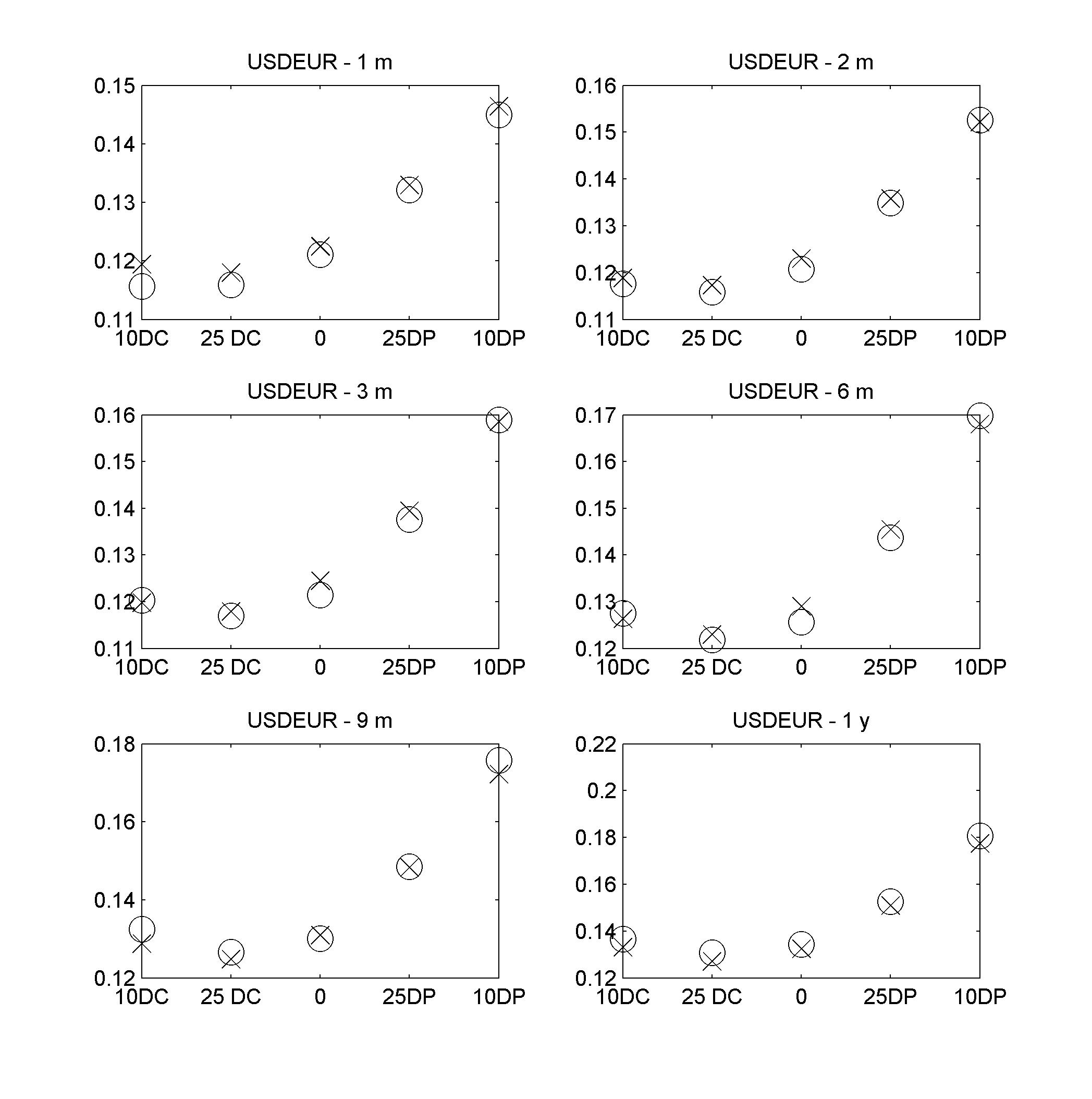
Figure 1: Calibration of the USD/EUR implied volatility surface. Market data as of 23/7/2010. Market volatilities are denoted by crosses, model volatilities are denoted by circles. Moneyness levels follow the standard Delta quoting convention in the FX option market, see Footnote 4. DC and DP stand for ”delta call” and ”delta put” respectively.

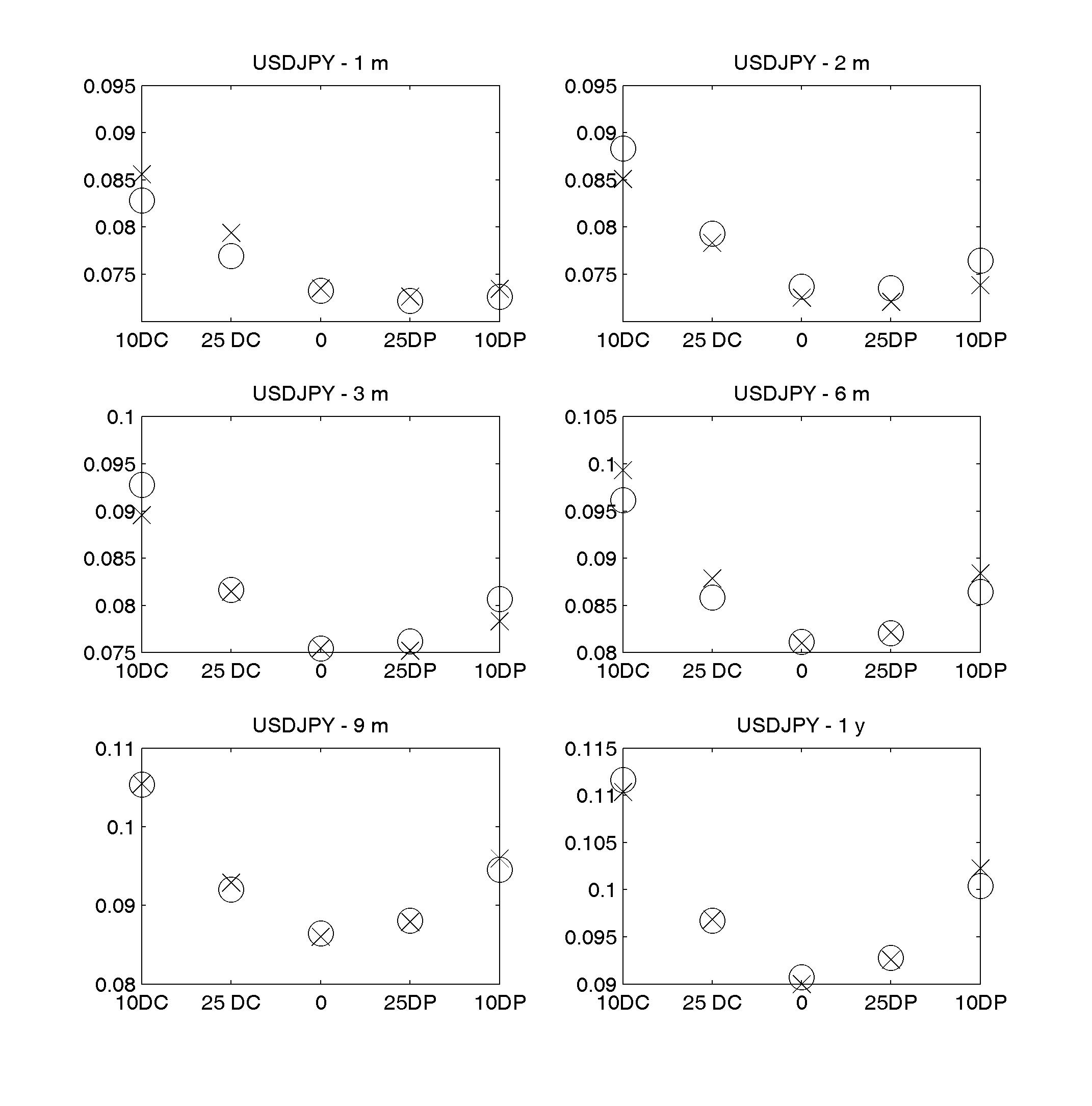
Figure 9: Calibration of the USD/JPY implied volatility surface. Market data as of 2/11/2012. Market volatilities are denoted by crosses, model volatilities are denoted by circles. Moneyness levels follow the standard Delta quoting convention in the FX option market, see Footnote 4. DC and DP stand for ”delta call” and ”delta put” respectively.

In this section we show an example of simultaneous calibration to three market volatility surfaces of options. We consider two currency triangles: EUR/USD/JPY as it appeared on the day 23/7/2010 and AUD/USD/JPY on 2/11/2012. Differences between the two sets of market data are due both to the different currency pair involved, e.g. replacing the EUR with the larger yield carry-trade AUD currency, and the different time-stamp. Note in particular the pronounced skew in the EURUSD volatility (bid for the EURUSD puts, see Fig. 1) during the European debt crisis in mid 2010 and the almost symmetric shape of the USDJPY volatilities, usually bid for the USDJPY puts, prior to BOJ currency easing efforts and the then ongoing USD rally in late 2012, see Fig. 9. For each of the two case studies we consider the implied volatility surfaces for each pair in the triangle, eg. for EUR/USD/JPY, the pairs USD/EUR, USD/JPY and EUR/JPY, that is $N=3$ with $i=\mathrm{USD};\ \mathrm{EUR};\ \mathrm{JPY}$. The volatility sample includes expiry dates ranging from 3 days to 5 years. The quotes follow the standard Delta quoting conversion in the FX option market, we have quotes on DN, 25 Delta, 15 Delta, and 10 Delta.

Let us concentrate here on the EUR/USD/JPY example, the other case follows the same procedure. We try to fit simultaneously the three volatility surfaces using two stochastic drivers, $d=2$. This choice yields a total number of parameters $N_{P}=16$, comparable to the number of parameters in 3 independent Heston models (15 parameters). This choice should not lead to overfitting instabilities. We work under the USD risk neutral measure to derive the option prices of the pairs EUR/USD and USD/JPY and the EUR measure for the EUR/JPY options, using (19). We calibrate the CIR parameters in the USD measure $\kappa_{k}^{\scriptscriptstyle\mathrm{USD}},\theta_{k}^{\scriptscriptstyle\mathrm{USD}},\xi_{k}^{\scriptscriptstyle\mathrm{USD}},\rho_{k}^{\scriptscriptstyle\mathrm{USD}},\ k=1,2$. The parameters for the EUR/JPY are transformed to the EUR measure through Eqs. (17) and the invariance property of correlation and vol-of-vol parameters.

The calibration is done via a standard non-linear least-squares optimizer that minimizes the total calibration error in terms of the difference between calibrated and target implied volatities $\sum_{n}(\sigma_{n,\mathrm{market}}^{\mathrm{imp}}-\sigma_{n,\mathrm{model}}^{\mathrm{imp}})^{2}$. The use of a norm in price should be avoided as the numerical range for option prices may be large, thus introducing a bias in the optimization. In fact, a norm in price penalizes greatly high prices, so that the fit for short maturity options (which are cheaper) is quite poor. For a more detailed discussion on the impact of the penalizing function on the calibrated parameters we refer to Christoffersen and Jacobs, (2004) and Da Fonseca and Grasselli, (2011).

5.2 Calibration results

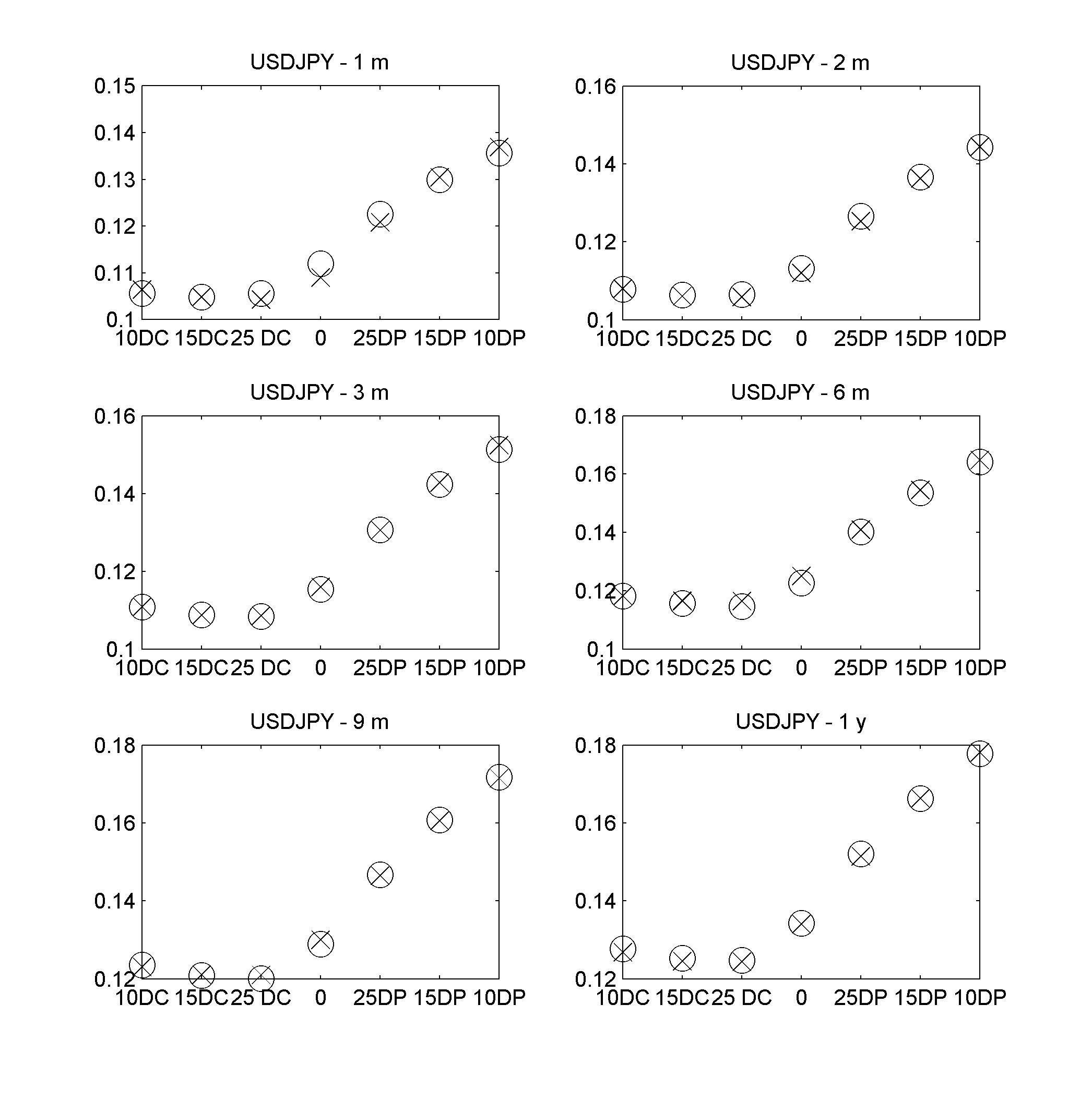
Figure 2: Calibration of the USD/JPY implied volatility surface. Market data as of 23/7/2010. Market volatilities are denoted by crosses, model volatilities are denoted by circles. Moneyness levels follow the standard Delta quoting convention in the FX option market, see Footnote 4. DC and DP stand for ”delta call” and ”delta put” respectively.

In Figs. 1, 2 and 3 we plot the market implied volatilities against those produced by the model. The plots refer to the largest sample in Table 1. Market volatilities are denoted by crosses, model volatilities are denoted by circles. The quality of the fit is comparable if not superior with respect to what is usually achieved by means of the standard Heston model for a single currency pair. The plots for the calibration on the sub-samples are completely analogous.

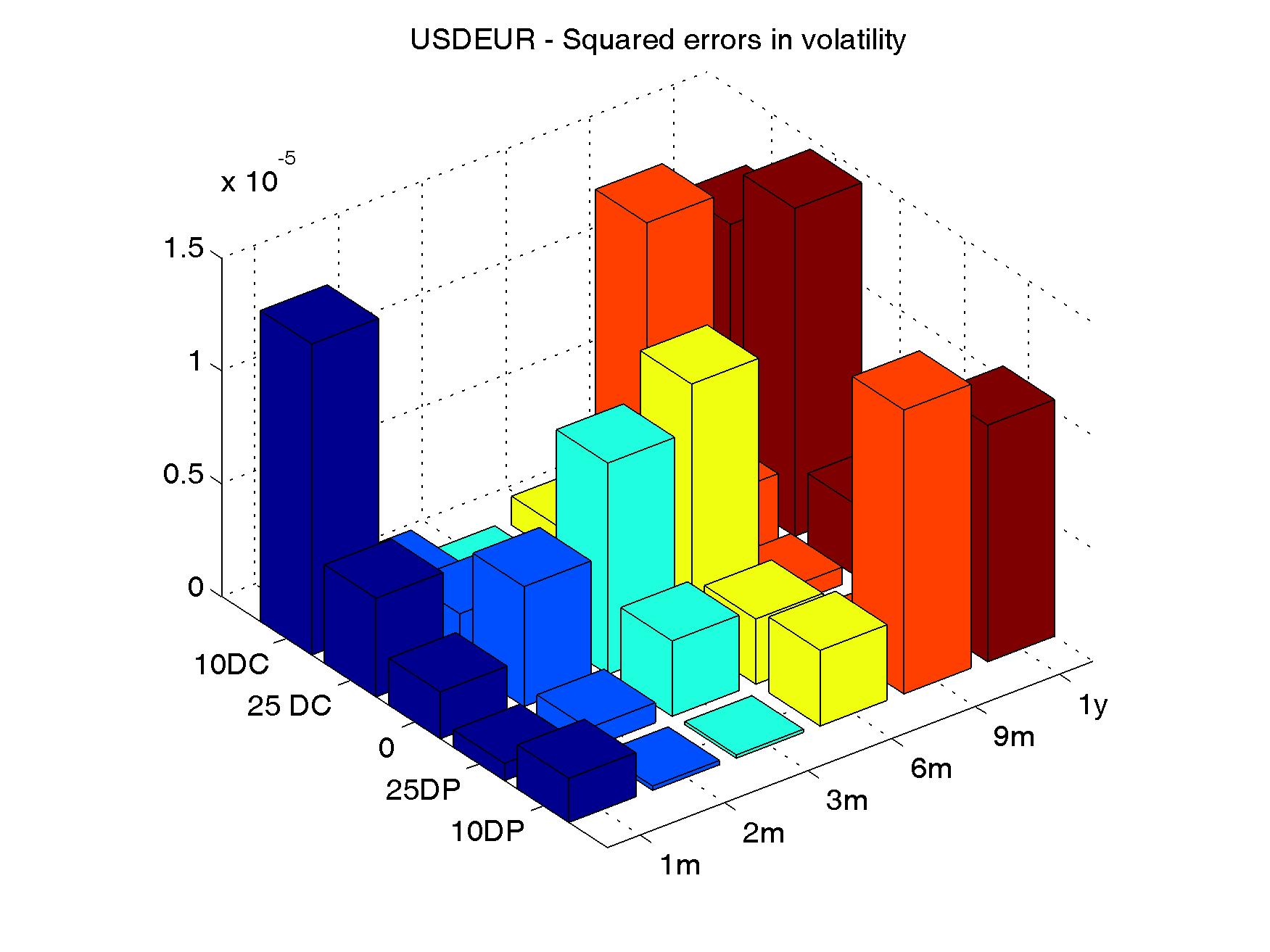
(a)

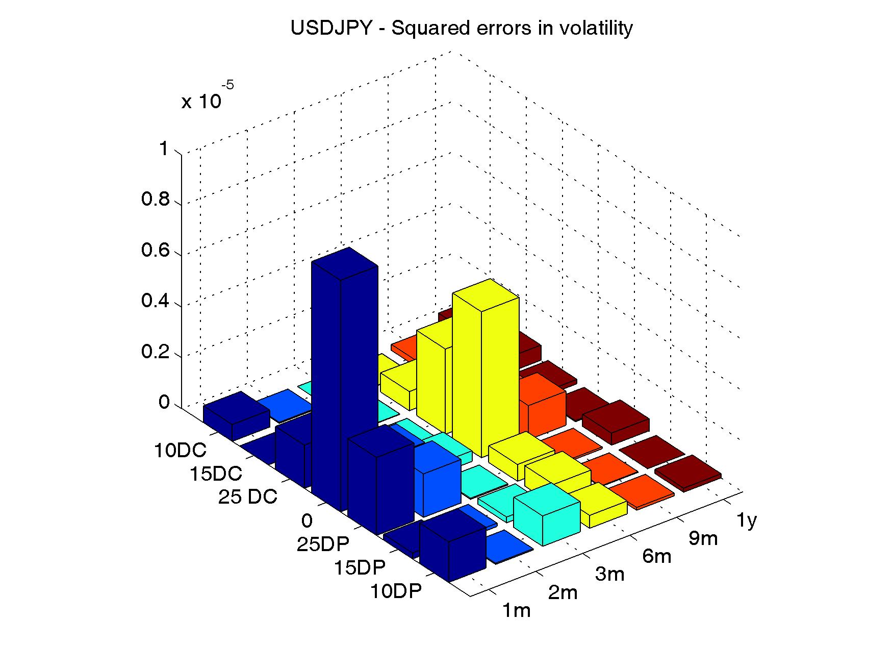
(b)

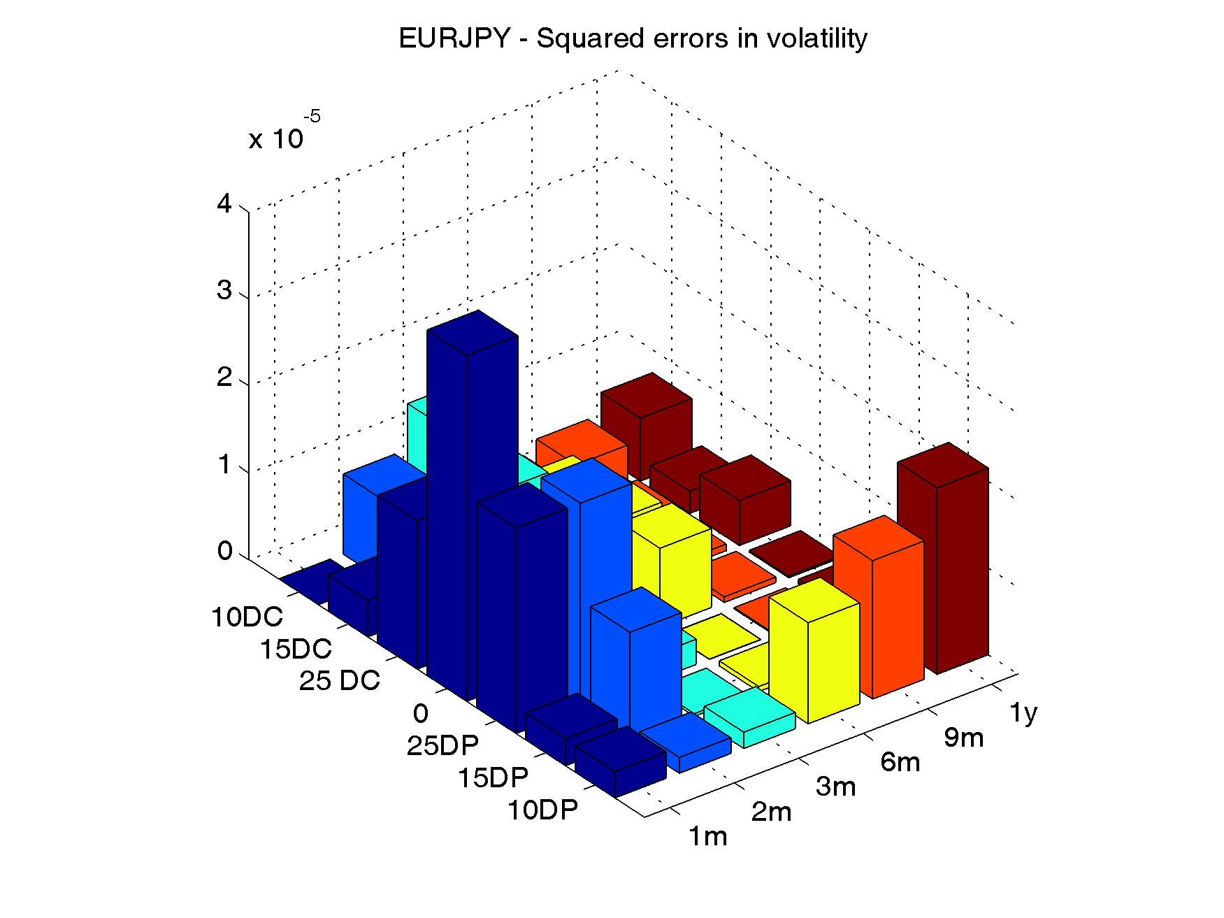
(c)

Figure 4: In-sample implied volatilities squared error for the joint calibration on 1m, 2m, 3m, 6m, 9m and 1y. The associated model parameters may be found in Table 1, column ”6”.

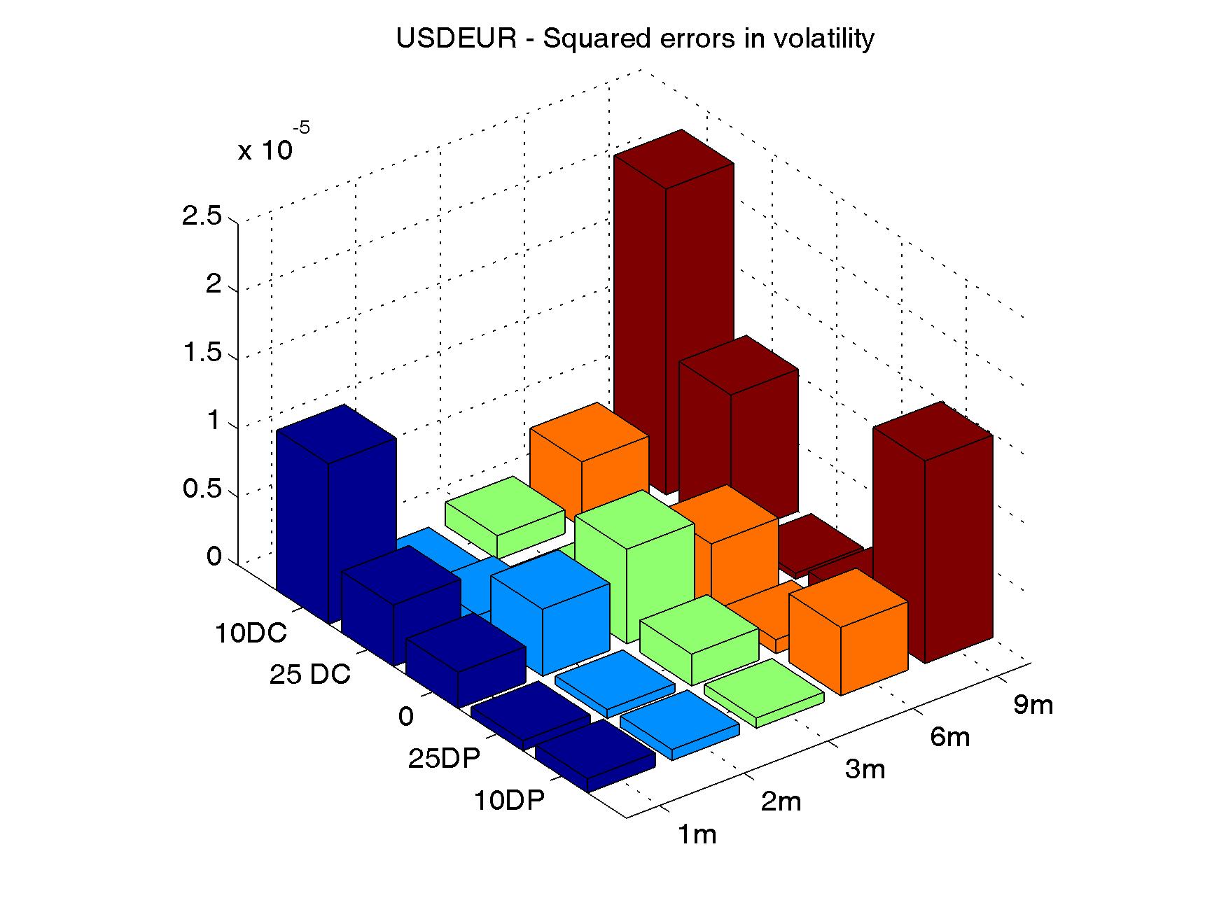
(a)

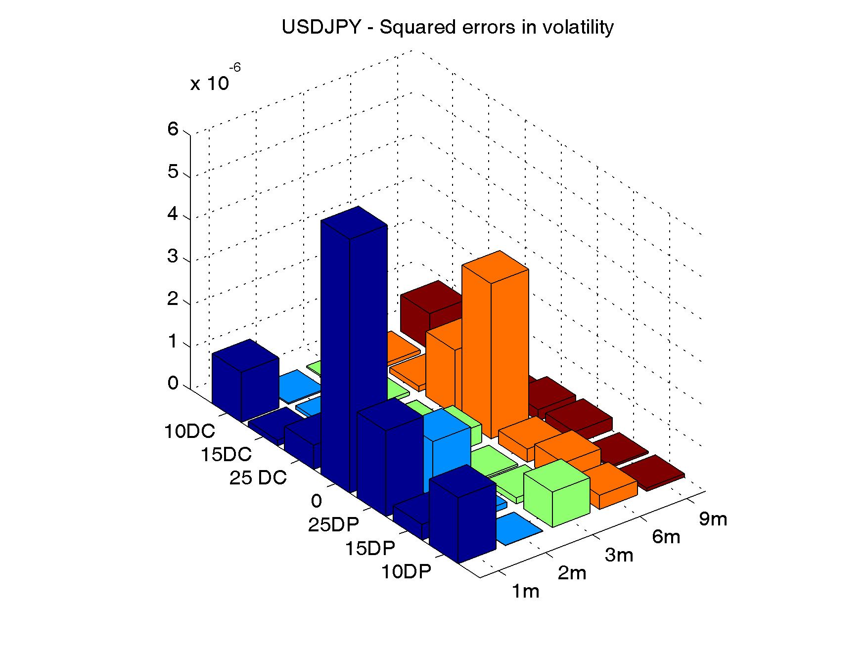
(b)

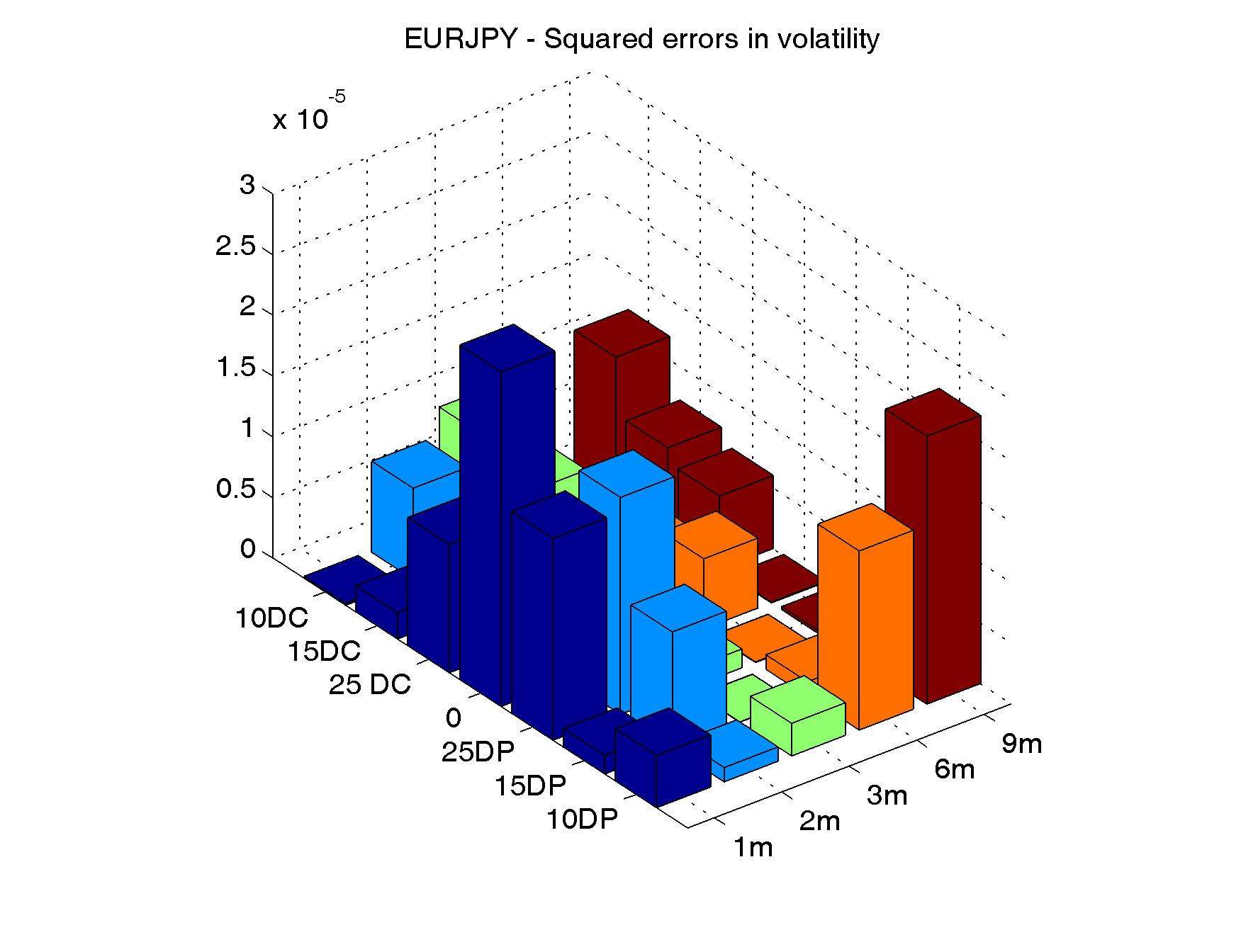
(c)

Figure 5: In-sample implied volatilities squared error for the joint calibration on 1m, 2m, 3m, 6m, and 9m. The associated model parameters may be found in Table 1, column ”5”.

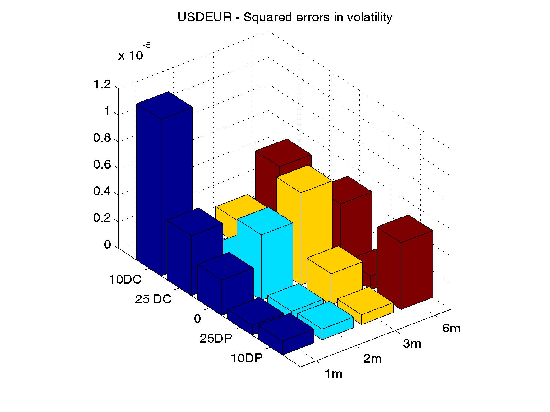
(a)

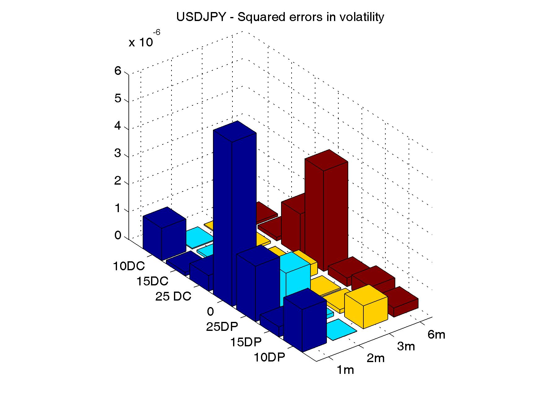
(b)

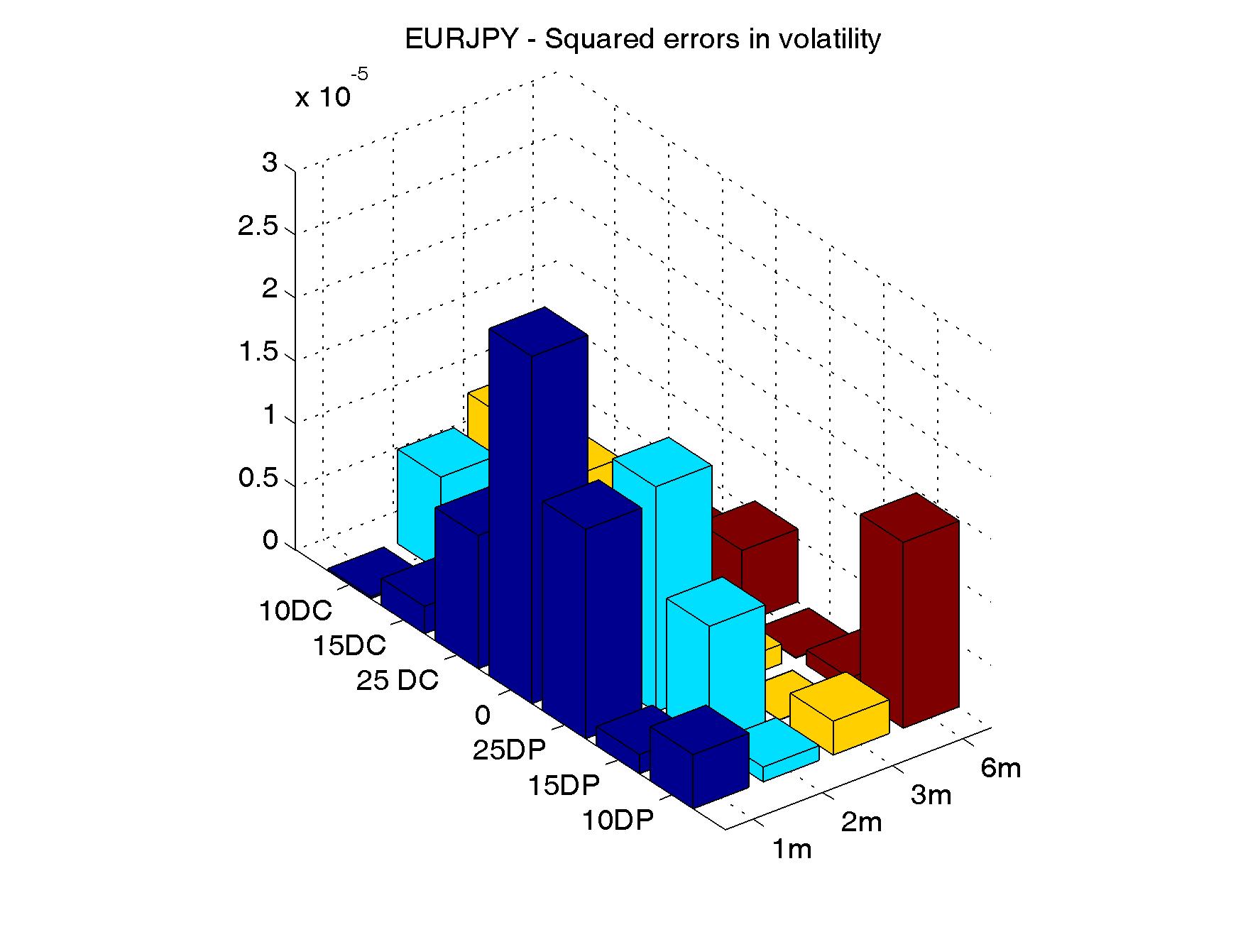
(c)

Figure 6: In-sample implied volatilities squared error for the joint calibration on 1m, 2m, 3m, and 6m. The associated model parameters may be found in Table 1, column ”4”.

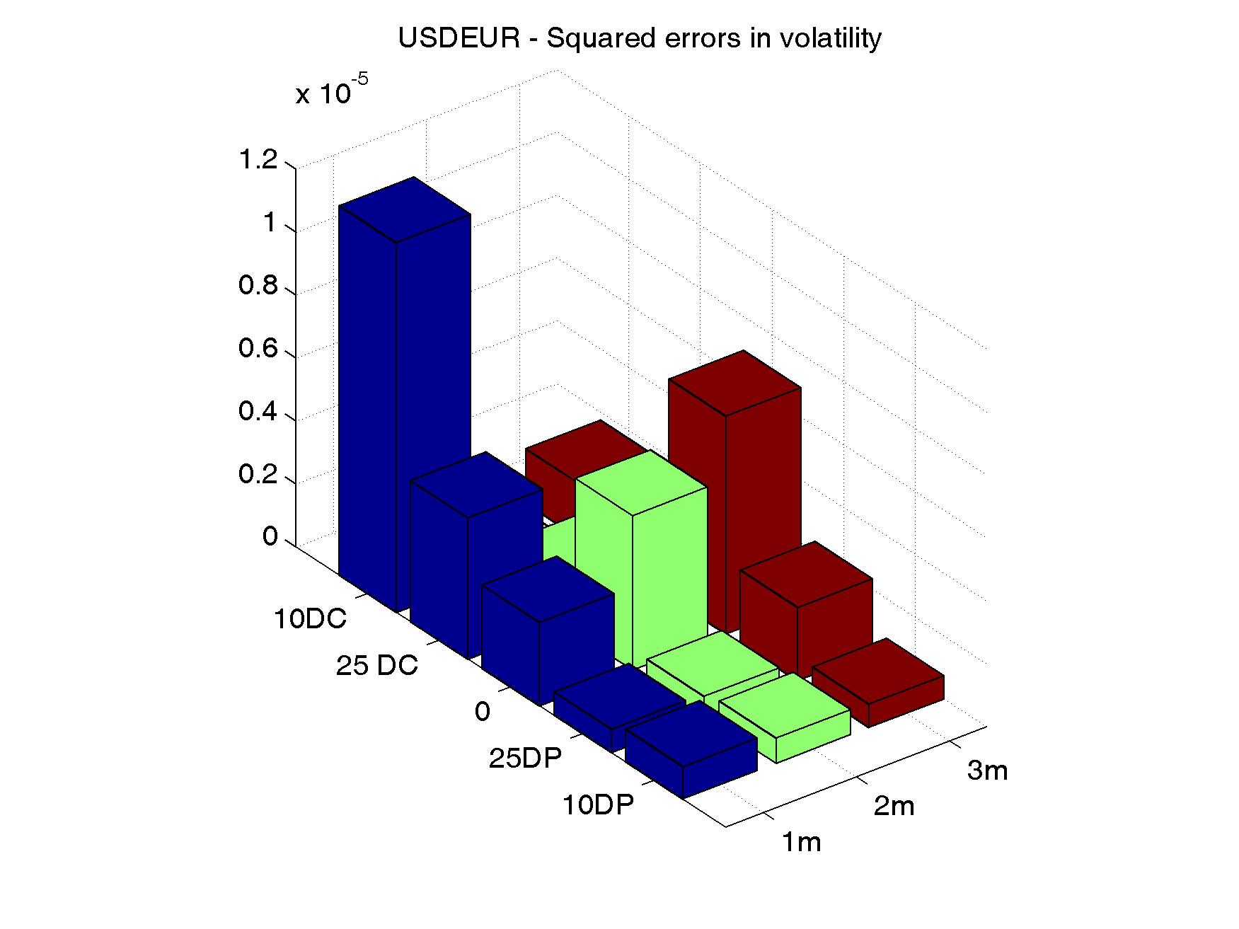
(a)

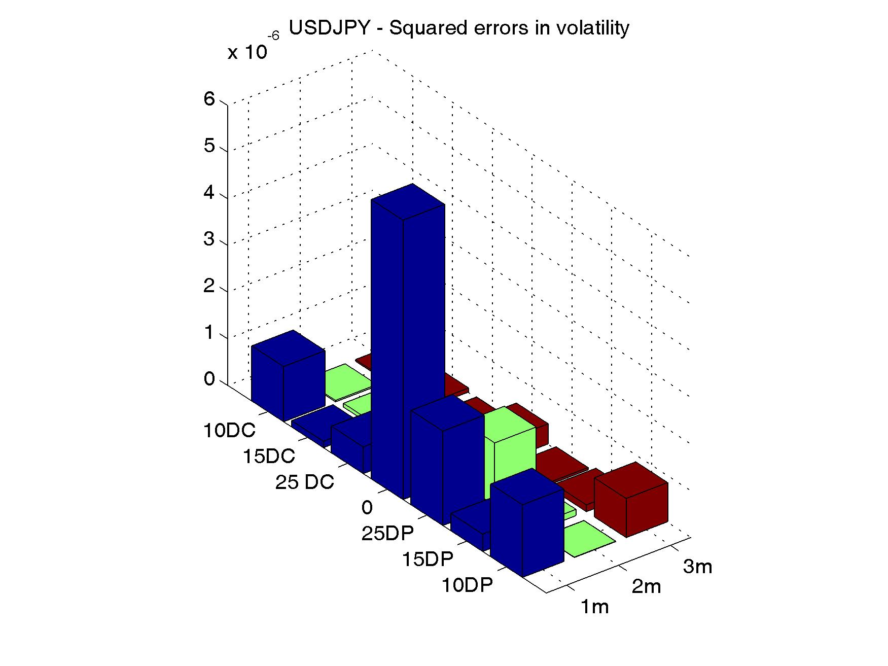
(b)

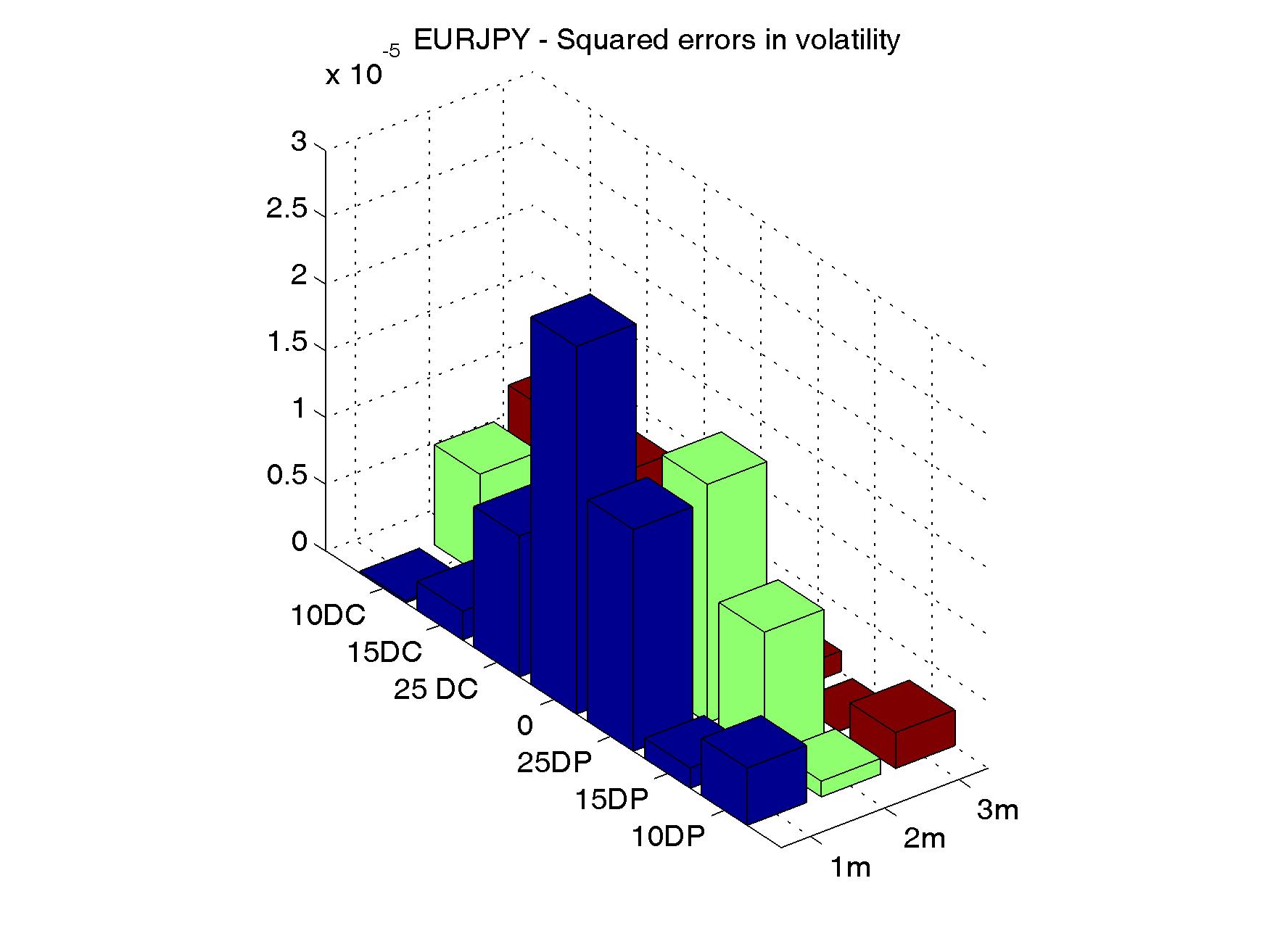
(c)

Figure 7: In-sample implied volatilities squared error for the joint calibration on 1m, 2m, and 3m. The associated model parameters may be found in Table 1, column ”3”.

In Table 1 we report the result of the calibration of the model for the EUR/USD/JPY triangle, whereas Fig. 4, reports the squared error in volatility for each moneyness/maturity. We have performed the optimization considering different sets of expiries. The expiries considered in the largest sample are the following: 1, 2, 3, 6, 9 months and 1 year. The result for this particular choice of expiries is reported in the first column on the left. Then we have repeated the experiment by excluding the largest expiry, 1 year. The result is reported in the second column. We proceed in this way by excluding more and more expiries. The smallest sample is reported in the last column and considers only options expiring in 1 and 2 months. In-sample squared errors in implied volatilities are visualized in Figs. 5, 6, 7 8.

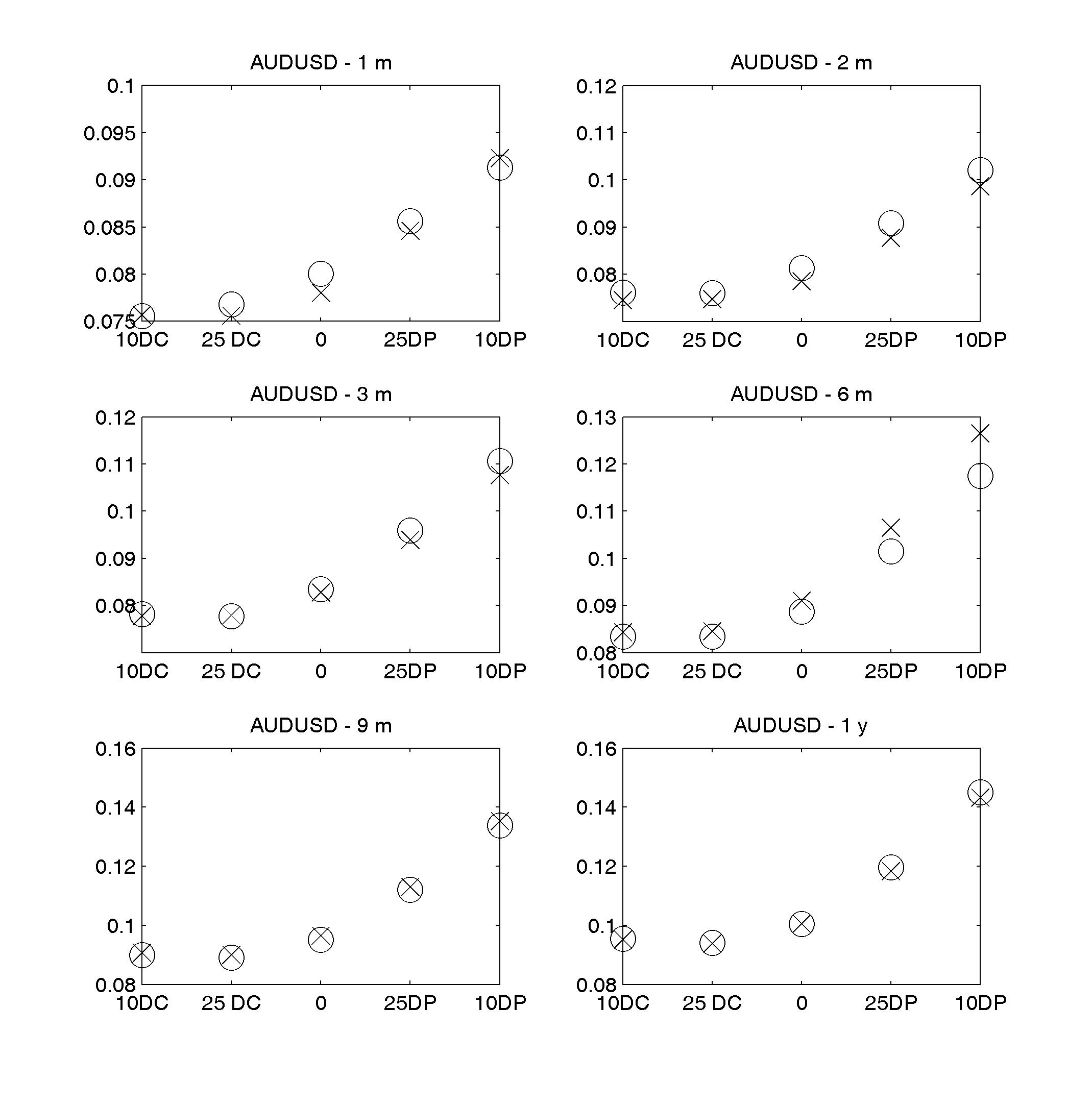
Figure 10: Calibration of the AUD/USD implied volatility surface. Market data as of 2/11/2012. Market volatilities are denoted by crosses, model volatilities are denoted by circles. Moneyness levels follow the standard Delta quoting convention in the FX option market, see Footnote 4. DC and DP stand for ”delta call” and ”delta put” respectively.

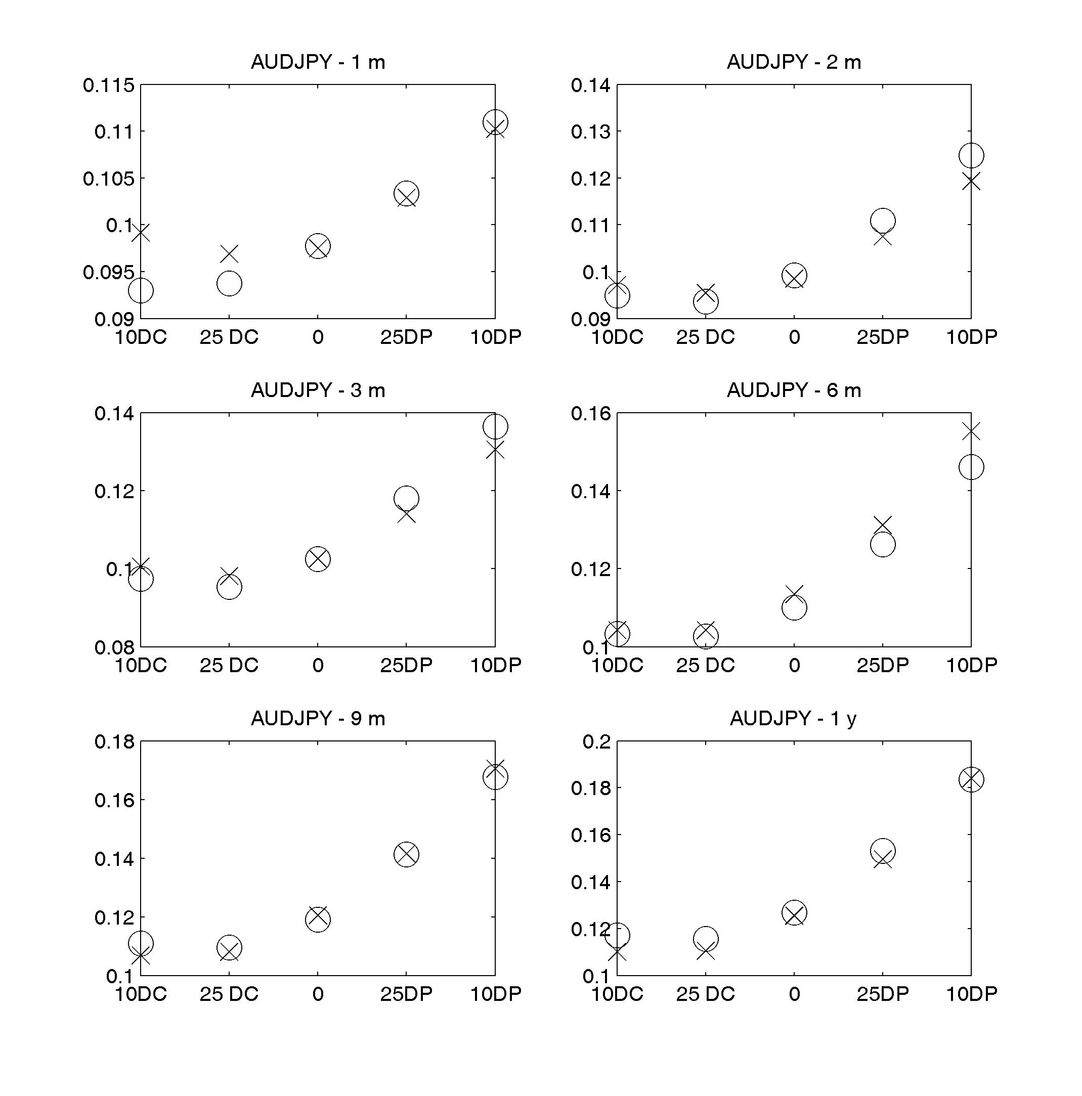
Figure 11: Calibration of the AUD/JPY implied volatility surface. Market data as of 2/11/2012. Market volatilities are denoted by crosses, model volatilities are denoted by circles. Moneyness levels follow the standard Delta quoting convention in the FX option market, see Footnote 4. DC and DP stand for ”delta call” and ”delta put” respectively.

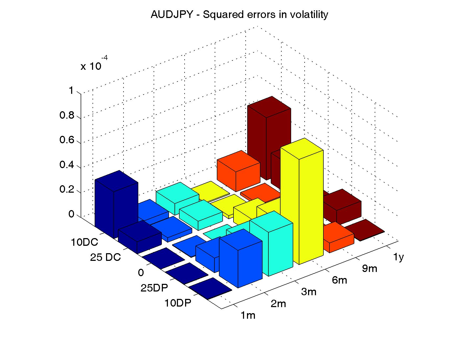
(c)

Figure 12: In-sample implied volatilities squared error for the joint calibration on 1m, 2m, 3m, 6m, 9m and 1y. The associated model parameters may be found in Table 15, column ”6”.

For the AUD/USD/JPY case, we limit ourselves to report in Figs. 9, 10 and 11 the result of the fit on the largest sample, consisting of implied volatilities at 1, 2, 3, 6, 9 months and 1 year. In Fig. 12 we show the squared errors in implied volatilities for each point of the surface that we are considering. We report in Table 15 the calibrated parameters. Also in this case the calibration yields a satisfactory fit to the market data.

5.3 Parameters stability tests

In this subsection we comment on the stability of the parameters via two different types of analysis. We first measure the impact on the parameters resulting from the calibration procedure. Secondly, we fit the model parameters to a certain sample and then use these parameters to price an option which is not included in the sample. If the out-of-sample prices are close to the market, the model gives a reasonable description of the joint underlying FX rates dynamics. Moreover, the calibration can be done on a limited set of expiries, reducing the computation effort of the optimizer.

As far as the first analysis is concerned, we show in Table 2 the relative variations computed with respect to the largest sample. With the exception of $\kappa_{1},\kappa_{2}$ we can see that there is a good degree of stability of the parameters across the sub-samples. Consequently, we perform also a second calibration experiment, where we fix $\kappa_{k}=1,k=1,2$. The results of this experiment are outlined in Table 3. The relative variation of the parameters can be found in Table 4. We notice that with this choice we get a good degree of stability, the most relevant fluctuation is now around 20% for $\theta_{1}$.

Let us now turn our attention to the out-of-sample exercise. In Tables 5, 6, 7 and 8 we show the difference between the market and the out-of-sample volatility for all sub-samples. The differences are always well below one volatility point.

5.4 Moment explosion

In this subsection we discuss some caveats coming from the parameters we obtained through the calibration procedure. It is known that for square root processes $0$ represents an attainable state when the Feller condition is not satisfied, that is when $2\kappa_{k}\theta_{k}<\xi_{k}^{2}$. In our modelling framework we have two volatility factors, hence we can perform the check for each factor. In Table 13 we report the quantity $F_{k}=2\kappa_{k}\theta_{k}-\xi_{k}^{2},k=1,2$. We observe violations of the Feller condition, which constitutes a well-known fact in the FX derivative practice, shared with the standard one-dimensional Heston model, see Clark, (2011). This phenomenon is strictly related to another established fact in stochastic volatility models, namely the pathological moment explosions which might often impact the stability of the pricing tools, see e.g. Andersen and Piterbarg, (2007), Keller-Ressel, (2011) and Glasserman and Kim, (2011). The model dynamics might lead to the explosion of moments, which become infinite in finite time. This fact might lead to complications/instabilities in standard numerical pricing routines mostly for large maturities. We can calculate the time of moment explosion for all currency pairs, see Andersen and Piterbarg, (2007). In Table 14 we consider moments up to order 5.

6 Conclusions

We have introduced a new multi-factor stochastic volatility Heston-based model that can provide an accurate joint description of multiple FX vanilla options across different currency pairs. The emphasis in the model specification has been in the preservation of the specific symmetries of FX markets. Differently from other asset classes, appropriate multiplications/divisions and inversions of FX rates are still FX rates. The choice of our simple CIR-based dynamics for the stochastic variance is instrumental in achieving this symmetry. We have indeed proven that our model is invariant with respect to the choice of the numéraire once the model parameters are appropriately transformed. The model is always of affine-type independently of which currency is used as risk free, leading to semi-analytical expression for all vanilla options between any of two currencies. This property is crucial when it comes to calibrating the model. In a standard global optimization algorithm we can consider together vanilla options in all currency pairs and achieve a simultaneous fit to the different volatility surfaces with reasonable computational effort.

The model shares naturally several stylized facts with the Heston model. The Feller condition is often violated when fitting the model to FX volatility surfaces, a common observation in the practice. Moreover, higher moments of the spot distribution explode at finite time; a property that might lead to complications/instabilities in standard numerical pricing routines mostly when maturities are large. Finally, like any pure stochastic volatility model, our model cannot be expected to deliver a perfect calibration of the vanilla surfaces across all Deltas and tenors, especially in the short end.

Having said that, the main result of the paper is a promising joint calibration of the model to the implied volatilities smiles of the EUR/USD/JPY and AUD/JPY/USD FX triangles. The fit remains satisfactory across the currency pairs, Deltas and tenors which were considered. Several in- and out-of-sample calibration studies in fact have proven the robustness of the calibration, especially once the mean reversion speed $\kappa$ has been fixed. Asymptotic expansions of the implied volatility surface are also included in the Appendix as they shed light on the meaning of the different model parameters and can help speeding up the calibration procedure by giving an educated guess for the initial parameters in the optimization procedure.

The price to pay in order to obtain a consistent simultaneous calibration to all volatilities surfaces is that the instantaneous volatilities of the currency pairs do not have single dedicated drivers. Their dynamics is rather brought about by a linear combination of several hidden stochastic factors. As in any principal component analysis, it is not easy to assign a financial meaning to each model parameter. As this study has shown, this appealing feature has most likely to be traded away in order to capture the complex phenomenology of the present global and widely interconnected FX markets.

7 Acknowledgements

We are grateful to Jan Baldeaux, Damiano Brigo, Imran Hafeez, Patrick Kuppinger, Eckhard Platen, Wolfgang Runggaldier and an anonymous referee for useful comments.

8 Images and Tables

8.1 Calibration of EUR/USD/JPY

	6	5	4	3	2
$V_{1}$	0.0137	0.0137	0.0136	0.0137	0.0135
$V_{2}$	0.0391	0.0365	0.0278	0.0293	0.0273
$a^{\scriptscriptstyle\mathrm{USD}}_{1}$	0.6650	0.6713	0.6165	0.6371	0.6518
$a^{\scriptscriptstyle\mathrm{USD}}_{2}$	1.0985	1.0531	0.9700	0.9795	0.9514
$a^{\scriptscriptstyle\mathrm{EUR}}_{1}$	1.6177	1.6222	1.5648	1.5804	1.6061
$a^{\scriptscriptstyle\mathrm{EUR}}_{2}$	1.3588	1.3208	1.2746	1.2797	1.2737
$a^{\scriptscriptstyle\mathrm{JPY}}_{1}$	0.2995	0.3151	0.2732	0.3035	0.3116
$a^{\scriptscriptstyle\mathrm{JPY}}_{2}$	1.6214	1.5922	1.5882	1.5858	1.5816
$\kappa_{1}$	0.9418	1.1432	1.5138	1.7349	1.8685
$\kappa_{2}$	1.7909	1.9998	1.9014	0.7142	0.7210
$\theta_{1}$	0.0370	0.0349	0.0329	0.0329	0.0297
$\theta_{2}$	0.0909	0.0839	0.0670	0.1236	0.1091
$\xi_{1}$	0.4912	0.5138	0.5542	0.5847	0.5962
$\xi_{2}$	1.0000	0.9997	0.8736	0.8318	0.8568
$\rho_{1}$	0.5231	0.5118	0.4916	0.4727	0.4567
$\rho_{2}$	-0.3980	-0.3956	-0.3943	-0.3902	-0.3728
Res. norm.	4.6996e-004	3.4244e-004	1.8618e-004	1.1145e-004	5.2514e-005

Table 1: This table reports the results of the calibration of the model. We concentrate on the two factor case. For each column, a different number of expiries, ranging from 6 to 2, is chosen. More specifically, 6 means that the following expiries are considered: 1, 2, 3, 6, 9 months and 1 year, whereas 5 means that the longest maturity, i.e. 1 year is excluded from the sample. We proceed analogously in the subsequent columns by excluding the longest expiry date up to the point where we perform the calibration on the 2-sample, where we fit the smile at 1 and 2 months. We consider market data as of 23rd July 2010. The reference exchange rates are $S^{\scriptscriptstyle\mathrm{JPY},\mathrm{EUR}}(0)=112.29$, $S^{\scriptscriptstyle\mathrm{USD},\mathrm{EUR}}(0)=1.2921$ and $S^{\scriptscriptstyle\mathrm{JPY},\mathrm{USD}}(0)=86.90$. Res. norm. is the residual of the objective function for the given set of parameters.

	5	4	3	2
$V_{1}$	0.1244%	-0.2866%	0.0960%	-1.1068%
$V_{2}$	-6.5645%	-28.9269%	-25.0960%	-30.0900%
$a^{\scriptscriptstyle\mathrm{USD}}_{1}$	0.9368%	-7.3035%	-4.1928%	-1.9883%
$a^{\scriptscriptstyle\mathrm{USD}}_{2}$	-4.1309%	-11.6957%	-10.8309%	-13.3918%
$a^{\scriptscriptstyle\mathrm{EUR}}_{1}$	0.2745%	-3.2714%	-2.3082%	-0.7190%
$a^{\scriptscriptstyle\mathrm{EUR}}_{2}$	-2.7989%	-6.1962%	-5.8255%	-6.2652%
$a^{\scriptscriptstyle\mathrm{JPY}}_{1}$	5.1809%	-8.8010%	1.3206%	4.0245%
$a^{\scriptscriptstyle\mathrm{JPY}}_{2}$	-1.7985%	-2.0460%	-2.1910%	-2.4522%
$\kappa_{1}$	21.3845%	60.7349%	84.2055%	98.3943%
$\kappa_{2}$	11.6649%	6.1715%	-60.1213%	-59.7402%
$\theta_{1}$	-5.6226%	-11.1784%	-11.0318%	-19.7810%
$\theta_{2}$	-7.7145%	-26.3082%	36.0430%	20.0453%
$\xi_{1}$	4.6020%	12.8359%	19.0424%	21.3784%
$\xi_{2}$	-0.0244%	-12.6344%	-16.8201%	-14.3193%
$\rho_{1}$	-2.1702%	-6.0305%	-9.6495%	-12.7003%
$\rho_{2}$	-0.6031%	-0.9375%	-1.9522%	-6.3351%

Table 2: In this table we consider the calibration on the largest sample as a basic case. We report the percentage difference between the model parameters resulting from the subsamples.

	6	5	4	3	2
$V_{1}$	0.0438	0.0430	0.0405	0.0421	0.0412
$V_{2}$	0.0465	0.0450	0.0408	0.0370	0.0335
$a^{\scriptscriptstyle\mathrm{USD}}_{1}$	0.7201	0.7165	0.7086	0.7099	0.7082
$a^{\scriptscriptstyle\mathrm{USD}}_{2}$	1.0211	1.0182	1.0095	0.9915	0.9685
$a^{\scriptscriptstyle\mathrm{EUR}}_{1}$	1.2517	1.2534	1.2603	1.2477	1.2538
$a^{\scriptscriptstyle\mathrm{EUR}}_{2}$	1.2624	1.2616	1.2619	1.2575	1.2589
$a^{\scriptscriptstyle\mathrm{JPY}}_{1}$	0.5159	0.5155	0.5093	0.5206	0.5142
$a^{\scriptscriptstyle\mathrm{JPY}}_{2}$	1.5053	1.5083	1.5223	1.5307	1.5372
$\theta_{1}$	0.1154	0.1169	0.1203	0.1391	0.1300
$\theta_{2}$	0.1344	0.1377	0.1350	0.1253	0.1081
$\xi_{1}$	0.8892	0.8898	0.8992	0.9700	0.9925
$\xi_{2}$	0.9338	0.9450	0.9458	0.9616	0.9659
$\rho_{1}$	0.5226	0.5132	0.4950	0.4756	0.4591
$\rho_{2}$	-0.4042	-0.4030	-0.4004	-0.3887	-0.3721
Res. Norm.	0.0013	4.7824e-04	1.9968e-04	2.6412e-04	4.7716e-04

Table 3: This table reports the results of the calibration of the model. In this case we are assuming $\kappa_{k}=1,k=1,2$. For each column, a different number of expiries, ranging from 6 to 2, is chosen. Res. norm. is the residual of the objective function for the given set of parameters.

	5	4	3	2
$V_{1}$	-1.8915%	-7.6930%	-3.8971%	-5.9284%
$V_{2}$	-3.1003%	-12.1687%	-20.3324%	-28.0033%
$a^{\scriptscriptstyle\mathrm{USD}}_{1}$	-0.5056%	-1.6003%	-1.4171%	-1.6497%
$a^{\scriptscriptstyle\mathrm{USD}}_{2}$	-0.2832%	-1.1348%	-2.9033%	-5.1535%
$a^{\scriptscriptstyle\mathrm{EUR}}_{1}$	0.1322%	0.6825%	-0.3164%	0.1703%
$a^{\scriptscriptstyle\mathrm{EUR}}_{2}$	-0.0691%	-0.0438%	-0.3903%	-0.2826%
$a^{\scriptscriptstyle\mathrm{JPY}}_{1}$	-0.0857%	-1.2718%	0.9087%	-0.3396%
$a^{\scriptscriptstyle\mathrm{JPY}}_{2}$	0.1994%	1.1235%	1.6872%	2.1131%
$\theta_{1}$	1.3740%	4.2649%	20.5911%	12.6966%
$\theta_{2}$	2.4412%	0.4181%	-6.8073%	-19.5908%
$\xi_{1}$	0.0622%	1.1246%	9.0864%	11.6096%
$\xi_{2}$	1.1985%	1.2881%	2.9747%	3.4434%
$\rho_{1}$	-1.7994%	-5.2886%	-8.9844%	-12.1501%
$\rho_{2}$	-0.2922%	-0.9392%	-3.8297%	-7.9304%

Table 4: In this table we consider the calibration on the largest sample as a basic case, when $\kappa_{k}=1,k=1,2$. We report the percentage difference between the model parameters resulting from the subsamples.

	USD/EUR	USD/JPY	EUR/JPY
10DC	-0.0006	-0.0002	-0.0027
15DC		0.0003	-0.0017
25DC	-0.0012	0.0005	-0.0005
0	-0.0022	0.0009	0.0021
25DP	-0.0008	0.0012	0.0042
15DP		0.0004	0.0031
10DP	0.0009	-0.0001	0.0011

Table 5: Out-of-sample performance. This table reports the raw difference between the market implied volatility and the model generated implied volatility for 1 year, when we calibrate the model to the previous 5 expiries. Moneyness levels follow the standard Delta quoting convention in the FX option market, see Footnote 4. DC and DP stand for ”delta call” and ”delta put” respectively. Blanks on the first column reflect missing market data for 15DC and 15DP.

	USD/EUR	USD/EUR	USD/JPY	USD/JPY	EUR/JPY	EUR/JPY
	9m	1y	9m	1y	9m	1y
10DC	-0.0031	0.0003	-0.0013	-0.0001	-0.0006	-0.0019
15DC			-0.0007	0.0002	0.0008	-0.0012
25DC	-0.0023	-0.0007	0.0004	0.0004	0.0021	-0.0006
0	-0.0021	-0.0021	0.0020	0.0006	0.0036	0.0012
25DP	-0.0010	-0.0007	0.0011	0.0010	0.0028	0.0033
15DP			-0.0008	0.0003	0.0004	0.0025
10DP	-0.0006	0.0015	-0.0014	-0.0000	-0.0026	0.0007

Table 6: Out-of-sample performance. This table reports the raw difference between the market implied volatility and the model generated implied volatility for 1 year and 9 months, when we calibrate the model to the previous 4 expiries. Moneyness levels follow the standard Delta quoting convention in the FX option market, see Footnote 4. DC and DP stand for ”delta call” and ”delta put” respectively. Blanks on the first two columns reflect missing market data for 15DC and 15DP.

		USD/EUR
	6m	9m	1y
10DC	-0.0060	-0.0023	0.0015
25DC	-0.0034	-0.0019	0.0002
0	-0.0018	-0.0020	-0.0017
25DP	-0.0006	-0.0010	-0.0005
10DP	0.0002	-0.0002	0.0019
		USD/JPY
	6m	9m	1y
10DC	-0.0058	-0.0011	0.0000
15DC	-0.0042	-0.0005	0.0002
25DC	-0.0009	0.0005	-0.0000
0	0.0016	0.0020	0.0000
25DP	0.0004	0.0009	0.0007
15DP	-0.0019	-0.0012	0.0002
10DP	-0.0037	-0.0020	-0.0002
		EUR/JPY
	6m	9m	1y
10DC	-0.0008	-0.0003	-0.0009
15DC	0.0011	0.0007	-0.0006
25DC	0.0031	0.0015	-0.0005
0	0.0041	0.0025	0.0006
25DP	0.0014	0.0018	0.0026
15DP	-0.0022	-0.0004	0.0019
10DP	-0.0053	-0.0032	0.0003

Table 7: Out-of-sample performance. This table reports the raw difference between the market implied volatility and the model generated implied volatility for 1 year, 9 and 6 months, when we calibrate the model to the previous 3 expiries. Moneyness levels follow the standard Delta quoting convention in the FX option market, see Footnote 4. DC and DP stand for ”delta call” and ”delta put” respectively.

		USD/EUR
	3m	6m	9m	1y
10DC	-0.0062	-0.0043	-0.0006	0.0031
25DC	-0.0027	-0.0022	-0.0007	0.0010
0	-0.0013	-0.0009	-0.0014	-0.0015
25DP	-0.0006	0.0001	-0.0005	-0.0005
10DP	0.0008	0.0009	0.0003	0.0020
		USD/JPY
	3m	6m	9m	1y
10DC	-0.0090	-0.0052	-0.0004	0.0007
15DC	-0.0062	-0.0038	-0.0002	0.0003
25DC	-0.0037	-0.0009	0.0003	-0.0006
0	0.0010	0.0014	0.0015	-0.0011
25DP	-0.0004	0.0006	0.0009	0.0002
15DP	-0.0022	-0.0014	-0.0008	0.0002
10DP	-0.0039	-0.0029	-0.0013	0.0003
		EUR/JPY
	3m	6m	9m	1y
10DC	-0.0045	-0.0003	0.0002	-0.0006
15DC	-0.0021	0.0014	0.0009	-0.0007
25DC	0.0010	0.0030	0.0012	-0.0013
0	0.0030	0.0038	0.0019	-0.0008
25DP	0.0009	0.0014	0.0014	0.0016
15DP	-0.0026	-0.0020	-0.0005	0.0013
10DP	-0.0057	-0.0050	-0.0030	-0.0000

Table 8: Out-of-sample performance. This table reports the raw difference between the market implied volatility and the model generated implied volatility for 1 year, 9, 6 and 3 months, when we calibrate the model to the previous 2 expiries. Moneyness levels follow the standard Delta quoting convention in the FX option market, see Footnote 4. DC and DP stand for ”delta call” and ”delta put” respectively.

	USD/EUR	USD/JPY	EUR/JPY
10DC	0.0058	0.0030	0.0046
15DC		0.0022	0.0035
25DC	0.0058	0.0009	0.0041
0	0.0035	0.0007	0.0019
25DP	0.0029	0.0024	0.0016
15DP		0.0027	-0.0012
10DP	0.0042	0.0029	-0.0044

Table 9: Out-of-sample performance. This table reports the raw difference between the market implied volatility and the model generated implied volatility for 1 year, when we calibrate the model to the previous 5 expiries and $\kappa_{k}=1,k=1,2$. Moneyness levels follow the standard Delta quoting convention in the FX option market, see Footnote 4. DC and DP stand for ”delta call” and ”delta put” respectively. Blanks on the first column reflect missing market data for 15DC and 15DP.

	USD/EUR	USD/EUR	USD/JPY	USD/JPY	EUR/JPY	EUR/JPY
	9m	1y	9m	1y	9m	1y
10DC	0.0083	0.0092	0.0034	0.0052	0.0073	0.0090
15DC			0.0021	0.0042	0.0061	0.0078
25DC	0.0060	0.0092	0.0005	0.0029	0.0053	0.0079
0	0.0029	0.0066	-0.0000	0.0025	0.0024	0.0050
25DP	0.0033	0.0056	0.0026	0.0044	0.0025	0.0041
15DP			0.0034	0.0049	0.0006	0.0010
10DP	0.0062	0.0067	0.0041	0.0054	-0.0027	-0.0024

Table 10: Out-of-sample performance. This table reports the raw difference between the market implied volatility and the model generated implied volatility for 1 year and 9 months, when we calibrate the model to the previous 4 expiries and $\kappa_{k}=1,k=1,2$. Moneyness levels follow the standard Delta quoting convention in the FX option market, see Footnote 4. DC and DP stand for ”delta call” and ”delta put” respectively. Blanks on the first two columns reflect missing market data for 15DC and 15DP.

		USD/EUR
	6m	9m	1y
10DC	0.0073	0.0116	0.0131
25DC	0.0042	0.0091	0.0128
0	0.0010	0.0056	0.0100
25DP	0.0020	0.0058	0.0087
10DP	0.0056	0.0088	0.0099
		USD/JPY
	6m	9m	1y
10DC	0.0025	0.0048	0.0067
15DC	0.0009	0.0030	0.0053
25DC	-0.0013	0.0008	0.0034
0	-0.0028	-0.0004	0.0023
25DP	0.0002	0.0027	0.0048
15DP	0.0013	0.0041	0.0057
10DP	0.0022	0.0053	0.0067
		EUR/JPY
	6m	9m	1y
10DC	0.0051	0.0114	0.0138
15DC	0.0036	0.0099	0.0123
25DC	0.0022	0.0085	0.0120
0	-0.0001	0.0048	0.0083
25DP	0.0017	0.0047	0.0071
15DP	0.0010	0.0028	0.0040
10DP	-0.0016	-0.0003	0.0006

Table 11: Out-of-sample performance. This table reports the raw difference between the market implied volatility and the model generated implied volatility for 1 year, 9 and 6 months, when we calibrate the model to the previous 3 expiries and $\kappa_{k}=1,k=1,2$. Moneyness levels follow the standard Delta quoting convention in the FX option market, see Footnote 4. DC and DP stand for ”delta call” and ”delta put” respectively.

		USD/EUR
	3m	6m	9m	1y
10DC	0.0057	0.0085	0.0125	0.0136
25DC	0.0023	0.0042	0.0086	0.0121
0	-0.0018	-0.0000	0.0041	0.0082
25DP	-0.0008	0.0010	0.0043	0.0068
10DP	0.0025	0.0050	0.0077	0.0086
		USD/JPY
	3m	6m	9m	1y
10DC	0.0013	0.0026	0.0046	0.0063
15DC	0.0004	0.0003	0.0020	0.0040
25DC	-0.0015	-0.0028	-0.0012	0.0010
0	-0.0033	-0.0051	-0.0033	-0.0010
25DP	-0.0010	-0.0015	0.0005	0.0022
15DP	-0.0004	0.0002	0.0025	0.0038
10DP	-0.0002	0.0017	0.0043	0.0053
		EUR/JPY
	3m	6m	9m	1y
10DC	0.0002	0.0048	0.0106	0.0127
15DC	-0.0009	0.0025	0.0082	0.0101
25DC	-0.0026	-0.0001	0.0056	0.0086
0	-0.0038	-0.0035	0.0008	0.0037
25DP	-0.0008	-0.0007	0.0016	0.0034
15DP	-0.0010	-0.0007	0.0005	0.0012
10DP	-0.0021	-0.0026	-0.0020	-0.0015

Table 12: Out-of-sample performance. This table reports the raw difference between the market implied volatility and the model generated implied volatility for 1 year, 9, 6 and 3 months, when we calibrate the model to the previous 2 expiries and $\kappa_{k}=1,k=1,2$. Moneyness levels follow the standard Delta quoting convention in the FX option market, see Footnote 4. DC and DP stand for ”delta call” and ”delta put” respectively.

	6	5	4	3	2
$k=1$	-0.1715	-0.1841	-0.2076	-0.2276	-0.2445
$k=2$	-0.6745	-0.6640	-0.5086	-0.5153	-0.5768

Table 13: For all $k=1,2$ and for each sample we report the quantity $2\kappa_{k}\theta_{k}-\xi_{k}^{2}$. In all cases the quantity is negative and its absolute value is a measure of the violation of the Feller condition.

Order	$S^{\scriptscriptstyle\mathrm{USD,EUR}}$	$S^{\scriptscriptstyle\mathrm{JPY,USD}}$	$S^{\scriptscriptstyle\mathrm{JPY,EUR}}$
1	$+\infty$	$+\infty$	$+\infty$
2	$+\infty$	12.1962	5.1612
3	$+\infty$	2.9537	2.0580
4	3.3968	1.7990	1.3763
5	2.0070	2.0819	1.0614

Table 14: Times of moment explosions for moments up to order 5 for the three currency pairs. First moments are always finite.

Figure 3: Calibration of the EUR/JPY implied volatility surface. Market data as of 23/7/2010. Market volatilities are denoted by crosses, model volatilities are denoted by circles. Moneyness levels follow the standard Delta quoting convention in the FX option market, see Footnote 4. DC and DP stand for ”delta call” and ”delta put” respectively.

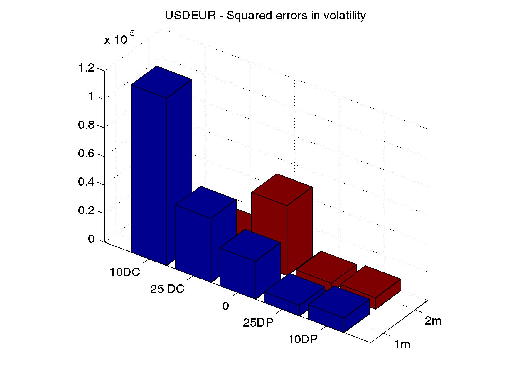
(a)

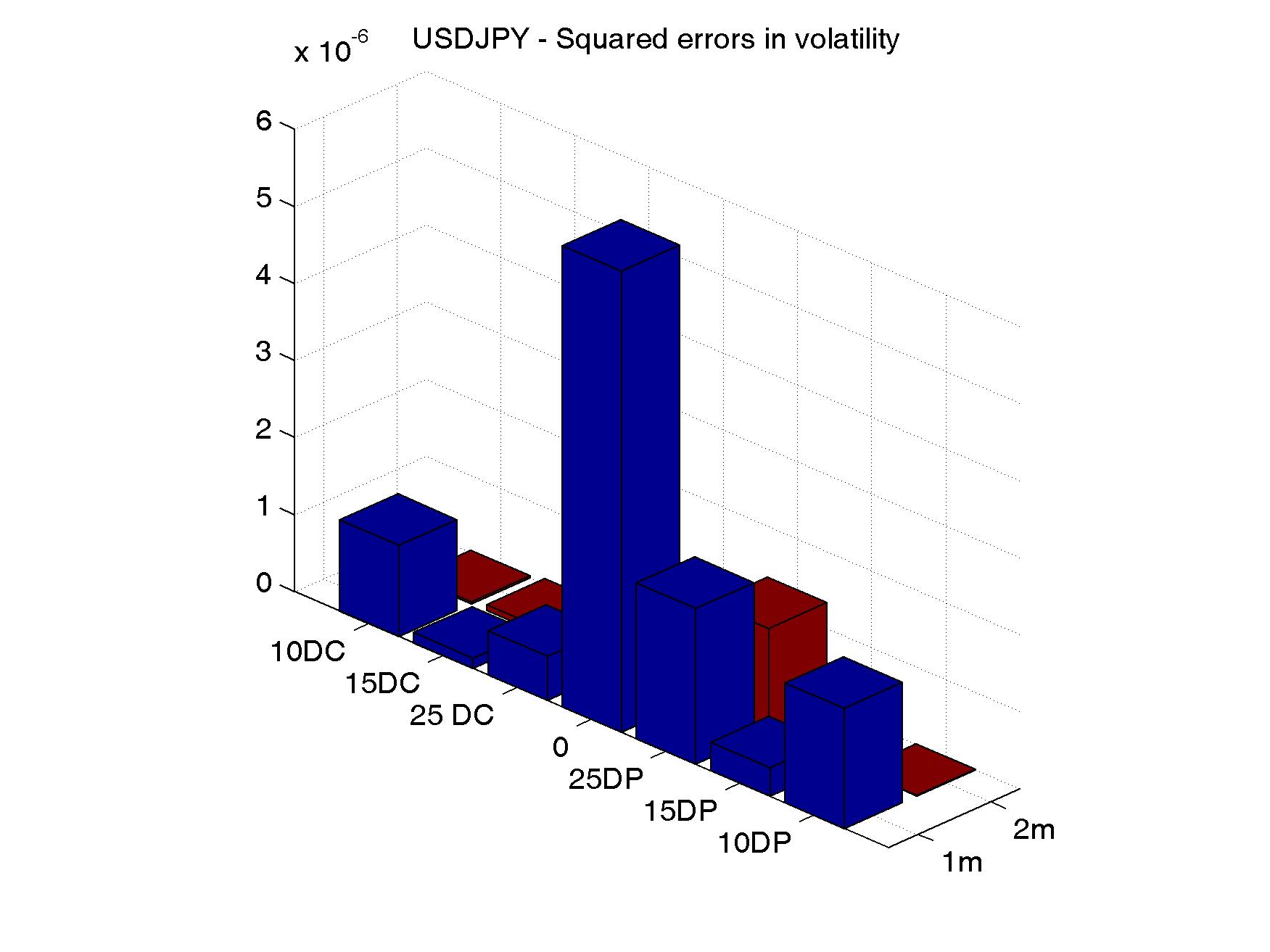
(b)

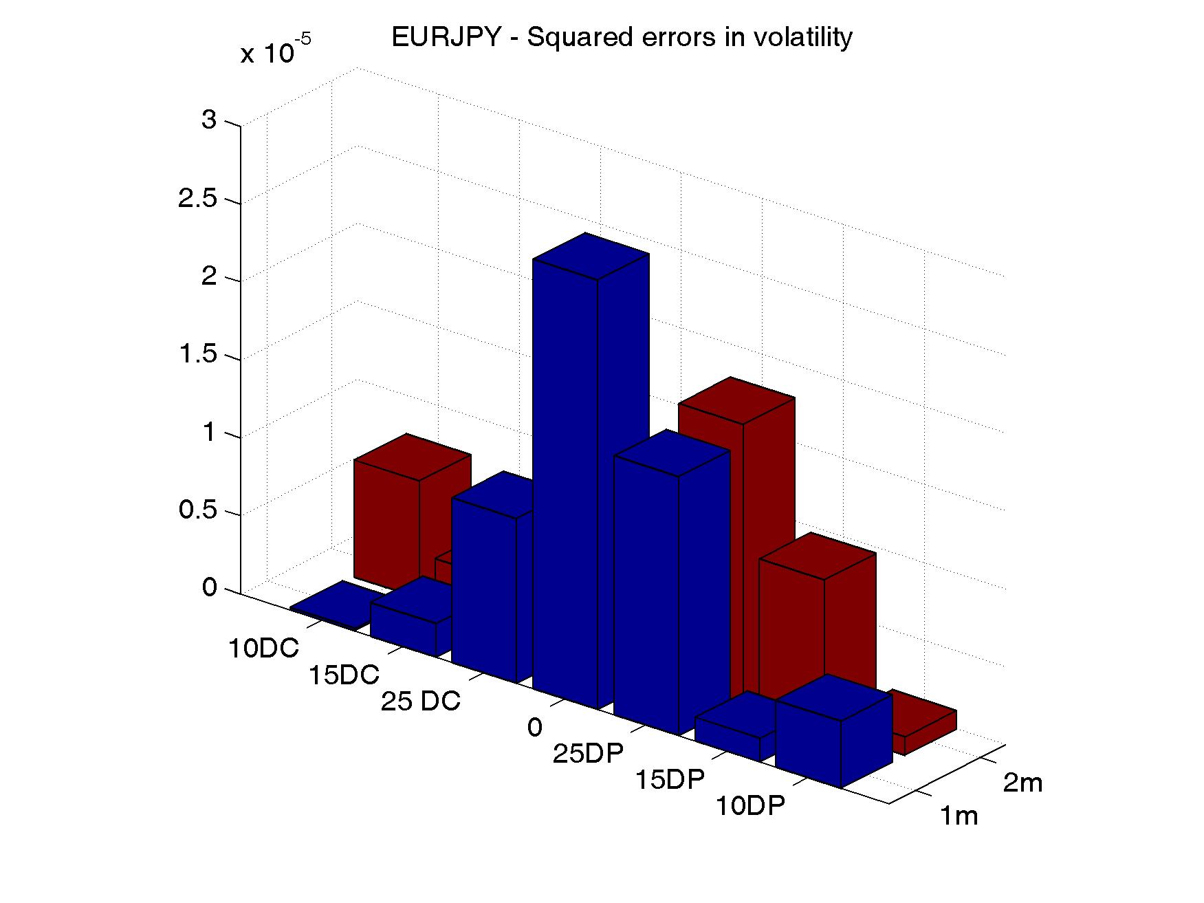
(c)

Figure 8: In-sample implied volatilities squared error for the joint calibration on 1m, and 2m. The associated model parameters may be found in Table 1, column ”2”.

8.2 Calibration of AUD/USD/JPY

	6	5	4	3	2
$V_{1}$	0.0115	0.0117	0.0109	0.0124	0.0133
$V_{2}$	0.0176	0.0159	0.0100	0.0196	0.0171
$a^{\scriptscriptstyle\mathrm{USD}}_{1}$	0.5142	0.5204	0.5097	0.5266	0.5184
$a^{\scriptscriptstyle\mathrm{USD}}_{2}$	1.3692	1.3757	1.4358	1.4075	1.3909
$a^{\scriptscriptstyle\mathrm{AUD}}_{1}$	0.8361	0.8179	0.7874	0.7681	0.7516
$a^{\scriptscriptstyle\mathrm{AUD}}_{2}$	0.7999	0.7789	0.6823	0.8455	0.7657
$a^{\scriptscriptstyle\mathrm{JPY}}_{1}$	1.2029	1.2047	1.2211	1.2159	1.2104
$a^{\scriptscriptstyle\mathrm{JPY}}_{2}$	1.5020	1.4957	1.5534	1.4756	1.4596
$\kappa_{1}$	1.9865	1.2988	0.2464	2.0000	2.0000
$\kappa_{2}$	0.8134	0.2298	0.0647	1.2270	1.8346
$\theta_{1}$	0.0314	0.0398	0.1351	0.0249	0.0182
$\theta_{2}$	0.0823	0.2332	0.5798	0.0608	0.0327
$\xi_{1}$	0.7196	0.6358	0.5264	0.5793	0.6086
$\xi_{2}$	1.0000	0.8956	0.7317	1.0000	1.0000
$\rho_{1}$	0.3337	0.3384	0.3408	0.3225	0.3283
$\rho_{2}$	-0.4451	-0.4455	-0.4416	-0.3910	-0.3834
Res. Norm.	8.2178e-04	7.6368e-04	0.0016	0.0010	5.4606e-05

Table 15: This table reports the results of the calibration of the model. We concentrate on the two factor case. For each column, a different number of expiries, ranging from 6 to 2, is chosen. More specifically, 6 means that the following expiries are considered: 1, 2, 3, 6, 9 months and 1 year, whereas 5 means that the longest maturity, i.e. 1 year is excluded from the sample. We proceed analogously in the subsequent columns by excluding the longest expiry date up to the point where we perform the calibration on the 2-sample, where we fit the smile at 1 and 2 months. We consider market data as of 2nd November 2012. The reference exchange rates are $S^{\scriptscriptstyle\mathrm{JPY},\mathrm{AUD}}(0)=83.29$, $S^{\scriptscriptstyle\mathrm{USD},\mathrm{AUD}}(0)=1.0375$ and $S^{\scriptscriptstyle\mathrm{JPY},\mathrm{USD}}(0)=80.28$.

(a)

(b)

9 Appendix A: The conditional Laplace transform

Recall that $\phi\left(\omega,t,\tau,x,\mathbf{V}\right)=G(\mathtt{i}\omega,t,\tau,x,\mathbf{V})$, with $x^{i,j}(t)=\log{S^{i,j}(t)}$. The functions $\phi,G$ represent resp. the characteristic function and the moment generating function of the log-exchange rate. In order to determine these quantities, we first need to write the PDE satisfied by $G$. First of all we write down the dynamics of $x=x^{i,j}$:

$$dx(t) =\left(\left(r^{i}-r^{j}\right)-\frac{1}{2}(\mathbf{a}^{i}-\mathbf{a}^{j})^{\top}\mathrm{Diag}\left(\mathbf{V}(t)\right)\left(\mathbf{a}^{i}-\mathbf{a}^{j}\right)\right)dt$$

$$+\left(\mathbf{a}^{i}-\mathbf{a}^{j}\right)^{\top}\sqrt{\mathrm{Diag}\left(\mathbf{V}(t)\right)}d\mathbf{Z}^{\mathbb{Q}^{i}}(t).$$ (25)

We also compute the following covariation terms for $k=1,..,d$:

$$d\left\langle x,V_{k}\right\rangle_{t} =d\left\langle\int_{0}^{.}\left(\mathbf{a}^{i}-\mathbf{a}^{j}\right)^{\top}\sqrt{\mathrm{Diag}\left(\mathbf{V}(u)\right)}d\mathbf{Z}^{\mathbb{Q}^{i}}(u),\int_{0}^{.}\xi_{k}\sqrt{V_{k}(u)}\rho_{k}dZ_{k}^{\mathbb{Q}^{i}}(u)\right\rangle_{t}$$

$$=d\left\langle\int_{0}^{.}\left(a^{i}_{k}-a^{j}_{k}\right)\sqrt{V_{k}(u)}dZ_{k}^{\mathbb{Q}^{i}}(u),\int_{0}^{.}\xi_{k}\sqrt{V_{k}(u)}\rho_{k}dZ_{k}^{\mathbb{Q}^{i}}(u)\right\rangle_{t}$$

$$=\left(a^{i}_{k}-a^{j}_{k}\right)V_{k}(t)\xi_{k}\rho_{k}dt.$$ (26)

The Laplace transform $G$ solves the following backward Kolmogorov equation Karatzas and Shreve, (1991):

$$-\frac{\partial G}{\partial t}=\frac{1}{2}\frac{\partial^{2}G}{\partial x^{2}}\left(\mathbf{a}^{i}-\mathbf{a}^{j}\right)^{\top}\mathrm{Diag}\left(\mathbf{V}\right)\left(\mathbf{a}^{i}-\mathbf{a}^{j}\right)$$

$$+\sum_{k=1}^{d}{\frac{\partial^{2}G}{\partial x\partial V_{k}}\left(a^{i}_{k}-a^{j}_{k}\right)V_{k}\xi_{k}\rho_{k}}+\frac{1}{2}\sum_{k=1}^{d}{\frac{\partial^{2}G}{\partial V_{k}^{2}}\xi_{k}^{2}V_{k}}$$

$$+\left(\left(r^{i}-r^{j}\right)-\frac{1}{2}\left(\mathbf{a}^{i}-\mathbf{a}^{j}\right)^{\top}\mathrm{Diag}\left(\mathbf{V}\right)\left(\mathbf{a}^{i}-\mathbf{a}^{j}\right)\right)\frac{\partial G}{\partial x}$$

$$+\sum_{k=1}^{d}{\frac{\partial G}{\partial V_{k}}\kappa_{k}\left(\theta_{k}-V_{k}\right)}$$ (27)

with terminal condition $G\left(\omega,T,0,x,\mathbf{V}\right)=e^{\omega x}$ with $\omega\in\mathbb{R}$. In order to solve this problem we look for an exponential affine solution of the form:

$$G\left(\omega,t,\tau,x,\mathbf{V}\right)=\exp\left(A(t,T)+\sum_{k=1}^{d}{B_{k}(t,T)V_{k}}+C(t,T)x\right),$$ (28)

for some deterministic functions $A,B_{k},C$ that may depend on both $t,T$. Upon substitution of the guess and recognition of the terms we obtain the following system of $d+2$ ODE’s:

$$\frac{\partial A}{\partial t}+\sum_{k=1}^{d}{B_{k}(t,T)\kappa_{k}\theta_{k}}+\left(r^{i}-r^{j}\right)C(t,T)=0;$$ (29)

$$\frac{\partial B_{k}}{\partial t}+\frac{1}{2}C^{2}(t,T)\left(a^{i}_{k}-a^{j}_{k}\right)^{2}+C(t,T)B_{k}(t,T)\left(a^{i}_{k}-a^{j}_{k}\right)\rho_{k}\xi_{k}$$

$$+\frac{1}{2}B_{k}^{2}(t,T)\xi_{k}^{2}-\frac{1}{2}\left(a^{i}_{k}-a^{j}_{k}\right)^{2}C(t,T)-B_{k}(t,T)\kappa_{k}=0;$$ (30)

$$\frac{\partial C}{\partial t}=0,$$ (31)

with terminal conditions: $A(T,T)=0,\quad B_{k}(T,T)=0,\quad C(T,T)=\omega$ for $k=1,..,d$. From (31) and its terminal condition, we deduce that $C(t,T)=\omega$ for $t\in[0,T]$, so we can rewrite the system as follows:

$$\frac{\partial A}{\partial t}+\sum_{k=1}^{d}{\kappa_{k}\theta_{k}B_{k}(t,T)}+\left(r^{i}-r^{j}\right)\omega=0;$$ (32)

$$\frac{\partial B_{k}}{\partial t}+\frac{1}{2}B_{k}^{2}(t,T)\xi_{k}^{2}+\left(-\kappa_{k}+\omega\left(a^{i}_{k}-a^{j}_{k}\right)\rho_{k}\xi_{k}\right)B_{k}(t,T)$$

$$+\frac{\omega^{2}-\omega}{2}\left(a^{i}_{k}-a^{j}_{k}\right)^{2}=0,\quad k=1,..,d.$$ (33)

Now for $k=1,..,d$ we assume that $B_{k}(t,T)$ can be written by means of a function $E_{k}(t,T)$ and set:

$$B_{k}(t,T)=\frac{\frac{\partial}{\partial t}E_{k}(t,T)}{\frac{\xi_{k}^{2}}{2}E_{k}(t,T)},$$ (34)

then the solution for (33) is:

$$B_{k}(t,T)=\frac{\left(\omega^{2}-\omega\right)}{2}\left(a^{i}_{k}-a^{j}_{k}\right)^{2}\frac{1-e^{-\sqrt{\Delta_{k}}(T-t)}}{\lambda_{k}^{+}e^{-\sqrt{\Delta_{k}}(T-t)}-\lambda_{k}^{-}},$$ (35)

with

$$\Delta_{k} =\left(-\kappa_{k}+\omega\left(a^{i}_{k}-a^{j}_{k}\right)\rho_{k}\xi_{k}\right)^{2}-\xi_{k}^{2}\left(\omega^{2}-\omega\right)\left(a^{i}_{k}-a^{j}_{k}\right)^{2}$$ (36)

$$\lambda_{k}^{\pm} =\frac{\left(-\kappa_{k}+\omega\left(a^{i}_{k}-a^{j}_{k}\right)\rho_{k}\xi_{k}\right)\pm\sqrt{\Delta_{k}}}{2}.$$ (37)

Equipped with the solution for $B_{k}(t,T)$ we can now compute $A(t,T)$ as follows:

$$A(T,T)-A(t,T) =\int_{t}^{T}{\frac{\partial}{\partial u}A(u,T)du}$$

$$A(t,T) =\int_{t}^{T}{\sum_{k=1}^{d}{\kappa_{k}\theta_{k}B_{k}(u,T)}+\left(r^{i}-r^{j}\right)\omega du}$$

$$=\left(r^{i}-r^{j}\right)\omega(T-t)+\sum_{k=1}^{d}{\kappa_{k}\theta_{k}\int_{t}^{T}{B_{k}(u,T)du}}$$

$$=\left(r^{i}-r^{j}\right)\omega(T-t)+\sum_{k=1}^{d}{\frac{2\kappa_{k}\theta_{k}}{\xi_{k}^{2}}\int_{t}^{T}{\frac{\frac{\partial}{\partial t}E_{k}(t,T)}{E_{k}(t,T)}du}},$$ (38)

which implies that the solution for $A(t,T)$ is

$$A(t,T) =\left(r^{i}-r^{j}\right)\omega(T-t)+\sum_{k=1}^{d}{\frac{2\kappa_{k}\theta_{k}}{\xi_{k}^{2}}\log{\frac{\lambda_{k}^{+}-\lambda_{k}^{-}}{\lambda_{k}^{+}e^{\lambda_{k}^{-}(T-t)}-\lambda_{k}^{-}e^{\lambda_{k}^{+}(T-t)}}}}$$

$$=\left(r^{i}-r^{j}\right)\omega(T-t)+\sum_{k=1}^{d}{A_{k}(t,T)},$$ (39)

where the functions $A_{k}(t,T)$ are implicitly defined by the last equality for $k=1,..,d$. Now we obtain the statement of the proposition once we replace $B^{i,j}_{k}(\tau)=B_{k}(t,T),A^{i,j}_{k}(\tau)=A_{k}(t,T)$ with $\tau=T-t$.

10 Appendix B: Expansions

The calibrations that were presented in Sec. 5 were performed using a deterministic gradient-based optimizers of the squared distance between the model implied volatilities and market ones. Model implied volatilities are extracted from the prices produced by the FFT routine. The success of the optimization routine might be jeopardized by the likely existence of multiple local minima. Hence, it is crucial to start with appropriate initial guess for the model parameters that are as close as possible to the global minimum. To this aim, approximate solutions for the option prices are very useful in providing good initial guesses for the parameters.

We present here an approximate expression for the option prices under the multi-Heston model which is asymptotically valid for small vol-of-vol parameters. The derivation of this formula, which is reported in the next Appendix, relies on arguments which may be found in Lewis, (2000) and Da Fonseca and Grasselli, (2011) (we drop all currency indices, it is intended that we are considering the $(i,j)$ FX pair).

Proposition 1.

Assume that all vol-of-vol parameters $\xi_{k},k=1,..,d$ have been scaled by the same factor $\alpha>0$. Then the call price $C(S(t),K,\tau)$ in the Multifactor Heston-based exchange model can be approximated in terms of the scale factor $\alpha$ by differentiating the Black Scholes formula $C_{\scriptscriptstyle\mathrm{BS}}\left(S(t),K,\sigma,\tau\right)$ with respect to the log exchange rate $x(t)=\ln S(t)$ and the integrated variance $v=\sigma^{2}\tau$:

$$C(S(t),K,\tau) \approx C_{\scriptscriptstyle\mathrm{BS}}\left(S(t),K,\sigma,\tau\right)$$

$$+\alpha\sum_{k=1}^{d}\left({\mathcal{A}_{k}^{(1)}(\tau)+\mathcal{B}_{k}^{(1)}(\tau)V_{k}}\right)\partial^{2}_{xv}C_{\scriptscriptstyle\mathrm{BS}}\left(S(t),K,\sigma,\tau\right)$$

$$+\alpha^{2}\sum_{k=1}^{d}\left({\mathcal{A}_{k}^{(2)}(\tau)+\mathcal{B}_{k}^{(2)}(\tau)V_{k}}\right)\partial^{2}_{vv}C_{\scriptscriptstyle\mathrm{BS}}\left(S(t),K,\sigma,\tau\right)$$

$$+\alpha^{2}\sum_{k=1}^{d}\left({\mathcal{A}_{k}^{(3)}(\tau)+\mathcal{B}_{k}^{(3)}(\tau)V_{k}}\right)\partial^{3}_{xxv}C_{\scriptscriptstyle\mathrm{BS}}\left(S(t),K,\sigma,\tau\right)$$

$$+\frac{\alpha^{2}}{2}\left[\sum_{k=1}^{d}\left({\mathcal{A}_{k}^{(1)}(\tau)+\mathcal{B}_{k}^{(1)}(\tau)V_{k}}\right)\right]^{2}\partial^{4}_{xxvv}C_{\scriptscriptstyle\mathrm{BS}}\left(S(t),K,\sigma,\tau\right).$$ (40)

We have defined $\tau=T-t$ and the auxiliary real deterministic functions $\mathcal{B}_{k}^{(0)},\mathcal{B}_{k}^{(1)},\mathcal{B}_{k}^{(2)},\mathcal{B}_{k}^{(3)},k=1,..,d$ as

$$\mathcal{B}_{k}^{(0)}(\tau) =\left(a^{i}_{k}-a^{j}_{k}\right)^{2}\frac{1-e^{-\kappa_{k}\tau}}{\kappa_{k}};$$ (41)

$$\mathcal{B}_{k}^{(1)}(\tau) =\left(a^{i}_{k}-a^{j}_{k}\right)^{3}\rho_{k}\xi_{k}\left(\frac{1}{\kappa_{k}^{2}}-\frac{e^{-\kappa_{k}\tau}}{\kappa_{k}^{2}}-\frac{\tau e^{-\kappa_{k}\tau}}{\kappa_{k}}\right);$$ (42)

$$\mathcal{B}_{k}^{(2)}(\tau) =\left(a^{i}_{k}-a^{j}_{k}\right)^{4}\frac{\xi_{k}^{2}}{2\kappa_{k}^{2}}\left(\frac{1-e^{-2\kappa_{k}\tau}}{\kappa_{k}}-2\tau e^{-\kappa_{k}\tau}\right);$$ (43)

$$\mathcal{B}_{k}^{(3)}(\tau) =\left(a^{i}_{k}-a^{j}_{k}\right)^{4}\rho_{k}^{2}\xi_{k}^{2}\left(\frac{1-e^{-\kappa_{k}\tau}}{\kappa_{k}^{3}}-\frac{\tau e^{-\kappa_{k}\tau}}{\kappa_{k}^{2}}-\frac{\tau^{2}e^{-\kappa_{k}\tau}}{2\kappa_{k}}\right)$$ (44)

and $\mathcal{A}_{k}^{(0)},\mathcal{A}_{k}^{(1)},\mathcal{A}_{k}^{(2)},\mathcal{A}_{k}^{(3)},k=1,..,d$ as

$$\mathcal{A}_{k}^{(0)}(\tau) =\left(a^{i}_{k}-a^{j}_{k}\right)^{2}\theta_{k}\left(\tau+\frac{e^{-\kappa_{k}\tau}-1}{\kappa_{k}}\right);$$ (45)

$$\mathcal{A}_{k}^{(1)}(\tau) =\left(a^{i}_{k}-a^{j}_{k}\right)^{3}\theta_{k}\rho_{k}\xi_{k}\left(\frac{\tau}{\kappa_{k}}+2\frac{e^{-\kappa_{k}\tau}-1}{\kappa_{k}^{2}}+\frac{\tau e^{-\kappa_{k}\tau}}{\kappa_{k}}\right);$$ (46)

$$\mathcal{A}_{k}^{(2)}(\tau) =\left(a^{i}_{k}-a^{j}_{k}\right)^{4}\theta_{k}\rho_{k}^{2}\xi_{k}^{2}\left(\frac{\tau}{\kappa_{k}}+\frac{e^{-\kappa_{k}\tau}-1}{\kappa_{k}^{3}}+\frac{\tau e^{-\kappa_{k}\tau}}{\kappa_{k}^{2}}\right.$$

$$\left.-\frac{e^{-\kappa_{k}\tau}-1}{\kappa_{k}^{2}}+\frac{\tau^{2}e^{-\kappa_{k}\tau}}{2\kappa_{k}}-\frac{\tau e^{-\kappa_{k}\tau}}{\kappa_{k}}+\frac{e^{-\kappa_{k}\tau}-1}{\kappa_{k}}\right);$$ (47)

$$\mathcal{A}_{k}^{(3)}(\tau) =\left(a^{i}_{k}-a^{j}_{k}\right)^{4}\theta_{k}\rho_{k}^{2}\xi_{k}^{2}\left(\frac{\tau}{\kappa_{k}^{2}}+3\frac{e^{-\kappa_{k}\tau}-1}{\kappa_{k}^{3}}+2\frac{\tau e^{-\kappa_{k}\tau}}{\kappa_{k}^{2}}+\frac{\tau^{2}e^{-\kappa_{k}\tau}}{2\kappa_{k}}\right).$$ (48)

Finally, the integrated variance reads

$$v=\sigma^{2}\tau=\sum_{k=1}^{d}\bigl{(}{\mathcal{A}_{k}^{(0)}(\tau)+\mathcal{B}_{k}^{(0)}(\tau)V_{k}}\bigr{)}.$$ (49)

Proof.

The starting point is given by the Riccati ODE (33) expressed in terms of time-to-maturity $\tau=T-t$ and perturbed by introducing the vol-of-vol scale parameter $\alpha$:

$$\frac{\partial B_{k}}{\partial\tau}=\frac{1}{2}B_{k}^{2}(\tau)\alpha^{2}\xi_{k}^{2}+\left(-\kappa_{k}+\omega\left(a^{i}_{k}-a^{j}_{k}\right)\rho_{k}\alpha\xi_{k}\right)B_{k}(\tau)$$

$$+\frac{\omega^{2}-\omega}{2}\left(a^{i}_{k}-a^{j}_{k}\right)^{2},\quad k=1,..,d.$$ (50)

We consider the following expansion in terms of $\alpha$: $B_{k}(\tau)=B_{k,0}(\tau)+\alpha B_{k,1}(\tau)+\alpha^{2}B_{k,2}(\tau)$. By plugging in the expansion and upon recognition of terms we obtain the following system of ODE’s:

$$\frac{\partial B_{k,0}}{\partial\tau} =-\kappa_{k}B_{k,0}(\tau)+\frac{\omega^{2}-\omega}{2}\left(a^{i}_{k}-a^{j}_{k}\right)^{2};$$ (51)

$$\frac{\partial B_{k,1}}{\partial\tau} =-\kappa_{k}B_{k,1}(\tau)+\omega\left(a^{i}_{k}-a^{j}_{k}\right)\rho_{k}\xi_{k}B_{k,0}(\tau);$$ (52)

$$\frac{\partial B_{k,2}}{\partial\tau} =-\kappa_{k}B_{k,2}(\tau)+\omega\left(a^{i}_{k}-a^{j}_{k}\right)\rho_{k}\xi_{k}B_{k,1}(\tau)+\frac{1}{2}B_{k,0}^{2}(\tau)\xi_{k}^{2}.$$ (53)

If we denote $\gamma:=\frac{\omega^{2}-\omega}{2}$ then the solutions are easily computed as:

$$B_{k,0}(\tau) =\underbrace{B_{k,0}(0)}_{=0}e^{-\kappa_{k}\tau}+e^{-\kappa_{k}\tau}\int_{0}^{\tau}{e^{\kappa_{k}u}\gamma\left(a^{i}_{k}-a^{j}_{k}\right)^{2}du}$$

$$=\gamma\mathcal{B}_{k}^{(0)}(\tau);$$ (54)

$$B_{k,1}(\tau) =\underbrace{B_{k,1}(0)}_{=0}e^{-\kappa_{k}\tau}+e^{-\kappa_{k}\tau}\int_{0}^{\tau}{e^{\kappa_{k}u}\omega\left(a^{i}_{k}-a^{j}_{k}\right)\rho_{k}\xi_{k}\gamma\mathcal{B}_{k}^{(0)}(u)du}$$

$$=\omega\gamma\mathcal{B}_{k}^{(1)}(\tau);$$ (55)

$$B_{k,2}(\tau) =\underbrace{B_{k,2}(0)}_{=0}e^{-\kappa_{k}\tau}+e^{-\kappa_{k}\tau}\int_{0}^{\tau}{e^{\kappa_{k}u}\omega^{2}\gamma\left(a^{i}_{k}-a^{j}_{k}\right)\rho_{k}\xi_{k}\mathcal{B}_{k}^{(1)}(u)du}$$

$$+e^{-\kappa_{k}\tau}\int_{0}^{\tau}{e^{\kappa_{k}u}\gamma\frac{\xi_{k}^{2}}{2}\left(\mathcal{B}_{k}^{(0)}(u)\right)^{2}du}$$

$$=\omega^{2}\gamma\mathcal{B}_{k}^{(3)}(\tau)+\gamma^{2}\mathcal{B}_{k}^{(2)}(\tau).$$ (56)

Then we can write the function $B_{k}(\tau)$ as follows:

$$B_{k}(\tau)=\gamma\mathcal{B}_{k}^{(0)}(\tau)+\alpha\omega\gamma\mathcal{B}_{k}^{(1)}(\tau)+\alpha^{2}\left(\omega^{2}\gamma\mathcal{B}_{k}^{(3)}(\tau)+\gamma^{2}\mathcal{B}_{k}^{(2)}(\tau)\right).$$ (57)

A direct substitution of (57) into (32) allows us to express the function $A(\tau)$:

$$A(\tau) =\omega\left(r^{i}-r^{j}\right)\tau+\sum_{k=1}^{d}{\kappa_{k}\theta_{k}\int_{0}^{\tau}B_{k}(u)du}$$

$$=\omega\left(r^{i}-r^{j}\right)\tau+\gamma\sum_{k=1}^{d}\underbrace{\kappa_{k}\theta_{k}\int_{0}^{\tau}{\mathcal{B}_{k}^{(0)}(u)}du}_{:=\mathcal{A}_{k}^{(0)}(\tau)}+\omega\gamma\alpha\sum_{k=1}^{d}\underbrace{\kappa_{k}\theta_{k}\int_{0}^{\tau}{\mathcal{B}_{k}^{(1)}(u)}du}_{:=\mathcal{A}_{k}^{(1)}(\tau)}$$

$$+\omega^{2}\gamma\alpha^{2}\sum_{k=1}^{d}\underbrace{\kappa_{k}\theta_{k}\int_{0}^{\tau}{\mathcal{B}_{k}^{(3)}(u)}du}_{:=\mathcal{A}_{k}^{(3)}(\tau)}+\alpha^{2}\gamma^{2}\sum_{k=1}^{d}\underbrace{\kappa_{k}\theta_{k}\int_{0}^{\tau}{\mathcal{B}_{k}^{(2)}(u)}du}_{:=\mathcal{A}_{k}^{(2)}(\tau)}.$$ (58)

We consider then the price in terms of Fourier transform as in (19) by replacing the argument $\omega=\mathtt{i}\lambda$. A Taylor-McLaurin expansion w.r.t. $\alpha$ gives the following:

$$C(S(t),K,\tau) \approx\frac{e^{-r^{i}\tau}}{2\pi}\int_{\mathcal{Z}}{e^{\mathtt{i}\lambda\left(r^{i}-r^{j}\right)\tau+\mathtt{i}\lambda x+\gamma\sum_{k=1}^{d}\left({\mathcal{A}_{k}^{(0)}(\tau)+\mathcal{B}_{k}^{(0)}(\tau)V_{k}}\right)}\Phi(\lambda)d\lambda}$$

$$+\alpha\sum_{k=1}^{d}\left({\mathcal{A}_{k}^{(1)}(\tau)+\mathcal{B}_{k}^{(1)}(\tau)V_{k}}\right)$$

$$\times\frac{e^{-r^{i}\tau}}{2\pi}\int_{\mathcal{Z}}{\gamma\mathtt{i}\lambda e^{\mathtt{i}\lambda\left(r^{i}-r^{j}\right)\tau+\mathtt{i}\lambda x+\gamma\sum_{k=1}^{d}\left({\mathcal{A}_{k}^{(0)}(\tau)+\mathcal{B}_{k}^{(0)}(\tau)V_{k}}\right)}\Phi(\lambda)d\lambda}$$

$$+\alpha^{2}\sum_{k=1}^{d}\left({\mathcal{A}_{k}^{(2)}(\tau)+\mathcal{B}_{k}^{(2)}(\tau)V_{k}}\right)$$

$$\times\frac{e^{-r^{i}\tau}}{2\pi}\int_{\mathcal{Z}}{\gamma^{2}e^{\mathtt{i}\lambda\left(r^{i}-r^{j}\right)\tau+\mathtt{i}\lambda x+\gamma\sum_{k=1}^{d}\left({\mathcal{A}_{k}^{(0)}(\tau)+\mathcal{B}_{k}^{(0)}(\tau)V_{k}}\right)}\Phi(\lambda)d\lambda}$$

$$+\alpha^{2}\sum_{k=1}^{d}\left({\mathcal{A}_{k}^{(3)}(\tau)+\mathcal{B}_{k}^{(3)}(\tau)V_{k}}\right)$$

$$\times\frac{e^{-r^{i}\tau}}{2\pi}\int_{\mathcal{Z}}{\gamma\mathtt{i}^{2}\lambda^{2}e^{\mathtt{i}\lambda\left(r^{i}-r^{j}\right)\tau+\mathtt{i}\lambda x+\gamma\sum_{k=1}^{d}\left({\mathcal{A}_{k}^{(0)}(\tau)+\mathcal{B}_{k}^{(0)}(\tau)V_{k}}\right)}\Phi(\lambda)d\lambda}$$

$$+\frac{\alpha^{2}}{2}\left[\sum_{k=1}^{d}\left({\mathcal{A}_{k}^{(1)}(\tau)+\mathcal{B}_{k}^{(1)}(\tau)V_{k}}\right)\right]^{2}$$

$$\times\frac{e^{-r^{i}\tau}}{2\pi}\int_{\mathcal{Z}}{\gamma^{2}\mathtt{i}^{2}\lambda^{2}e^{\mathtt{i}\lambda\left(r^{i}-r^{j}\right)\tau+\mathtt{i}\lambda x+\gamma\sum_{k=1}^{d}\left({\mathcal{A}_{k}^{(0)}(\tau)+\mathcal{B}_{k}^{(0)}(\tau)V_{k}}\right)}\Phi(\lambda)d\lambda}.$$

Recall now from (49) the definition of the integrated Black-Scholes variance. In the previous formula, in the first term on the right hand side, we recognise the Black-Scholes price in terms of the characteristic function when the integrated variance is $v=\sigma^{2}\tau$:

$$C_{\scriptscriptstyle\mathrm{BS}}\left(S(t),K,\sigma,\tau\right)=\frac{e^{-r^{i}\tau}}{2\pi}\int_{\mathcal{Z}}{e^{\mathtt{i}\lambda\left(r^{i}-r^{j}\right)\tau+\mathtt{i}\lambda x+\frac{(\mathtt{i}\lambda)^{2}-\mathtt{i}\lambda}{2}v}\Phi(\lambda)d\lambda},$$ (60)

so that the price expansion is of the form

$$C(S(t),K,\tau) \approx C_{\scriptscriptstyle\mathrm{BS}}\left(S(t),K,\sigma,\tau\right)$$

$$+\alpha\sum_{k=1}^{d}\left({\mathcal{A}_{k}^{(1)}(\tau)+\mathcal{B}_{k}^{(1)}(\tau)V_{k}}\right)\partial^{2}_{xv}C_{\scriptscriptstyle\mathrm{BS}}\left(S(t),K,\sigma,\tau\right)$$

$$+\alpha^{2}\sum_{k=1}^{d}\left({\mathcal{A}_{k}^{(2)}(\tau)+\mathcal{B}_{k}^{(2)}(\tau)V_{k}}\right)\partial^{2}_{vv}C_{\scriptscriptstyle\mathrm{BS}}\left(S(t),K,\sigma,\tau\right)$$

$$+\alpha^{2}\sum_{k=1}^{d}\left({\mathcal{A}_{k}^{(3)}(\tau)+\mathcal{B}_{k}^{(3)}(\tau)V_{k}}\right)\partial^{3}_{xxv}C_{\scriptscriptstyle\mathrm{BS}}\left(S(t),K,\sigma,\tau\right)$$

$$+\frac{\alpha^{2}}{2}\left[\sum_{k=1}^{d}\left({\mathcal{A}_{k}^{(1)}(\tau)+\mathcal{B}_{k}^{(1)}(\tau)V_{k}}\right)\right]^{2}\partial^{4}_{xxvv}C_{\scriptscriptstyle\mathrm{BS}}\left(S(t),K,\sigma,\tau\right).$$ (61)

From the previous expression we can deduce the relation defining the deterministic functions $\mathcal{B}_{k}^{(h)},\mathcal{A}_{k}^{(h)},\ h=0,...,3$.

$$\mathcal{B}_{k}^{(0)}(\tau) =\left(a^{i}_{k}-a^{j}_{k}\right)^{2}\frac{1-e^{-\kappa_{k}\tau}}{\kappa_{k}};$$ (62)

$$\mathcal{B}_{k}^{(1)}(\tau) =\left(a^{i}_{k}-a^{j}_{k}\right)\rho_{k}\xi_{k}e^{-\kappa_{k}\tau}\int_{0}^{\tau}{e^{\kappa_{k}u}\mathcal{B}_{k}^{(0)}(u)du};$$ (63)

$$\mathcal{B}_{k}^{(2)}(\tau) =\frac{\xi_{k}^{2}}{2\kappa_{k}}e^{-\kappa_{k}\tau}\int_{0}^{\tau}{e^{\kappa_{k}u}\left(\mathcal{B}_{k}^{(0)}(u)\right)^{2}du};$$ (64)

$$\mathcal{B}_{k}^{(3)}(\tau) =\left(a^{i}_{k}-a^{j}_{k}\right)\rho_{k}\xi_{k}e^{-\kappa_{k}\tau}\int_{0}^{\tau}{e^{\kappa_{k}u}\mathcal{B}_{k}^{(1)}(u)du}$$ (65)

and

$$\mathcal{A}_{k}^{(0)}(\tau) =\kappa_{k}\theta_{k}\int_{0}^{\tau}{\mathcal{B}_{k}^{(0)}(u)du};$$ (66)

$$\mathcal{A}_{k}^{(1)}(\tau) =\kappa_{k}\theta_{k}\int_{0}^{\tau}{\mathcal{B}_{k}^{(1)}(u)du};$$ (67)

$$\mathcal{A}_{k}^{(2)}(\tau) =\kappa_{k}\theta_{k}\int_{0}^{\tau}{\mathcal{B}_{k}^{(2)}(u)du};$$ (68)

$$\mathcal{A}_{k}^{(3)}(\tau) =\kappa_{k}\theta_{k}\int_{0}^{\tau}{\mathcal{B}_{k}^{(3)}(u)du}.$$ (69)

Computing the trivial integrals completes the proof.

∎

We can now present another formula, which does not involve the computation of option prices, and constitutes an approximation of the implied volatility surface for a short time to maturity. This formula may constitute a useful alternative in order to get a quicker calibration for short maturities and provides a good initial guess for the parameters in the calibration routine. The proof is again provided in detail in the next Appendix.

Proposition 2.

For a short time to maturity the implied volatility expansion in terms of the vol-of-vol scale factor $\alpha$ in the multifactor Heston-based exchange model is given by:

$$\sigma_{\mathrm{imp}}^{2}\approx \ \sigma_{0}^{2}+\alpha\left(\sum_{k=1}^{d}{\frac{\rho_{k}\xi_{k}}{2}\left(a^{i}_{k}-a^{j}_{k}\right)^{4}V_{k}}\right)\frac{m_{f}}{\sigma_{0}^{2}}$$

$$+ \ \alpha^{2}\frac{m_{f}^{2}}{12\left(\sigma_{0}^{2}\right)^{2}}\left[\sum_{k=1}^{d}\left(1+2\rho_{k}^{2}\right)\xi_{k}^{2}\left(a^{i}_{k}-a^{j}_{k}\right)^{4}V_{k}-\frac{15}{4\sigma_{0}^{2}}\left(\sum_{k=1}^{d}{\rho_{k}\xi_{k}\left(a^{i}_{k}-a^{j}_{k}\right)^{3}V_{k}}\right)^{2}\right],$$

where $\sigma_{0}^{2}=\left(\mathbf{a}^{i}-\mathbf{a}^{j}\right)^{\top}\mathrm{Diag}(\mathbf{V})\left(\mathbf{a}^{i}-\mathbf{a}^{j}\right)$ and $m_{f}=\log\left(\frac{S^{i,j}e^{(r^{i}-r^{j})\tau}}{K^{i,j}}\right)$ denotes the forward log-moneyness.

Proof.

We follow the procedure in Da Fonseca and Grasselli, (2011). We suppose an expansion for the integrated implied variance of the form $v=\sigma^{2}_{\mathrm{imp}}\tau=\zeta_{0}+\alpha\zeta_{1}+\alpha^{2}\zeta_{2}$ and we consider the Black-Scholes formula as a function of the integrated implied variance and the log exchange rate $x=\log S$: $C_{\scriptscriptstyle\mathrm{BS}}\left(S(t),K,\sigma,\tau\right)=C_{\scriptscriptstyle\mathrm{BS}}\left(x(t),K,\sigma_{imp}^{2}\tau,\tau\right)$. A Taylor-McLaurin expansion gives us the following:

$$C_{\scriptscriptstyle\mathrm{BS}}\left(x(t),K,\sigma_{imp}^{2}\tau,\tau\right) =C_{\scriptscriptstyle\mathrm{BS}}\left(x(t),K,\zeta_{0},\tau\right)+\alpha\zeta_{1}\partial_{v}C_{\scriptscriptstyle\mathrm{BS}}\left(x(t),K,\zeta_{0},\tau\right)$$

$$+\frac{\alpha^{2}}{2}\left(2\zeta_{2}\partial_{v}C_{\scriptscriptstyle\mathrm{BS}}\left(x(t),K,\zeta_{0},\tau\right)+\zeta_{1}^{2}\partial^{2}_{v^{2}}C_{\scriptscriptstyle\mathrm{BS}}\left(x(t),K,\zeta_{0},\tau\right)\right).$$ (70)

By comparing this with the price expansion (61) we deduce that the coefficients must be of the form:

$$\zeta_{0} =v_{0};$$ (71)

$$\zeta_{1} =\frac{\sum_{k=1}^{d}\left({\mathcal{A}_{k}^{(1)}(\tau)+\mathcal{B}_{k}^{(1)}(\tau)V_{k}}\right)\partial^{2}_{xv}C_{\scriptscriptstyle\mathrm{BS}}}{\partial_{v}C_{\scriptscriptstyle\mathrm{BS}}};$$ (72)

$$\zeta_{2} =\frac{-\zeta_{1}^{2}\partial^{2}_{vv}C_{\scriptscriptstyle\mathrm{BS}}+2\sum_{k=1}^{d}\left({\mathcal{A}_{k}^{(2)}(\tau)+\mathcal{B}_{k}^{(2)}(\tau)V_{k}}\right)\partial^{2}_{vv}C_{\scriptscriptstyle\mathrm{BS}}}{2\partial_{v}C_{\scriptscriptstyle\mathrm{BS}}}$$

$$+\frac{2\sum_{k=1}^{d}\left({\mathcal{A}_{k}^{(3)}(\tau)+\mathcal{B}_{k}^{(3)}(\tau)V_{k}}\right)\partial^{3}_{xxv}C_{\scriptscriptstyle\mathrm{BS}}+\left[\sum_{k=1}^{d}\left({\mathcal{A}_{k}^{(1)}(\tau)+\mathcal{B}_{k}^{(1)}(\tau)V_{k}}\right)\right]^{2}\partial^{4}_{xxvv}C_{\scriptscriptstyle\mathrm{BS}}}{2\partial_{v}C_{\scriptscriptstyle\mathrm{BS}}},$$ (73)

where the Black-Scholes formula $C_{\scriptscriptstyle\mathrm{BS}}\left(x(t),K,\sigma_{imp}^{2}\tau,\tau\right)$ is evaluated at the point $\left(x,K,v_{0},\tau\right)$. In order to find the values of $\zeta_{1},\zeta_{2}$, we differentiate (41)-(44) thus obtaining the following ODE’s:

$$\frac{\partial\mathcal{B}_{k}^{(0)}}{\partial\tau} =-\kappa_{k}\mathcal{B}_{k}^{(0)}(\tau)+\left(a^{i}_{k}-a^{j}_{k}\right)^{2};$$

$$\frac{\partial\mathcal{B}_{k}^{(1)}}{\partial\tau} =-\kappa_{k}\mathcal{B}_{k}^{(1)}(\tau)+\left(a^{i}_{k}-a^{j}_{k}\right)\rho_{k}\xi_{k}\mathcal{B}_{k}^{(0)}(\tau);$$

$$\frac{\partial\mathcal{B}_{k}^{(2)}}{\partial\tau} =-\kappa_{k}\mathcal{B}_{k}^{(2)}(\tau)+\frac{1}{2}\xi_{k}^{2}\mathcal{B}_{k}^{(0)}(\tau)^{2};$$

$$\frac{\partial\mathcal{B}_{k}^{(3)}}{\partial\tau} =-\kappa_{k}\mathcal{B}_{k}^{(3)}(\tau)+\left(a^{i}_{k}-a^{j}_{k}\right)\rho_{k}\xi_{k}\mathcal{B}_{k}^{(1)}(\tau).$$

We consider a Taylor-McLaurin expansion in terms of $\tau$:

$$\mathcal{B}_{k}^{(0)}(\tau) =\left(a^{i}_{k}-a^{j}_{k}\right)^{2}\tau-\frac{\tau^{2}}{2}\kappa_{k}\left(a^{i}_{k}-a^{j}_{k}\right)^{2};$$ (74)

$$\mathcal{B}_{k}^{(1)}(\tau) =\frac{\tau^{2}}{2}\left(a^{i}_{k}-a^{j}_{k}\right)^{3}\rho_{k}\xi_{k}-\frac{2}{3}\tau^{3}\kappa_{k}\left(a^{i}_{k}-a^{j}_{k}\right)^{3}\rho^{k}\xi^{k};$$ (75)

$$\mathcal{B}_{k}^{(2)}(\tau) =\frac{\tau^{3}}{6}\xi_{k}^{2}\left(a^{i}_{k}-a^{j}_{k}\right)^{4};$$ (76)

$$\mathcal{B}_{k}^{(3)}(\tau) =\frac{\tau^{3}}{6}\left(a^{i}_{k}-a^{j}_{k}\right)^{4}\rho_{k}^{2}\xi_{k}^{2}.$$ (77)

Noting from (45)-(48) that $\mathcal{A}_{k}^{(i)}$ are one order in $\tau$ higher than the corresponding $\mathcal{B}_{k}^{(i)}$, the following approximations hold:

$$\sum_{k=1}^{d}\left({\mathcal{A}_{k}^{(0)}(\tau)+\mathcal{B}_{k}^{(0)}(\tau)V_{k}}\right) =\sum_{k=1}^{d}{\left(a^{i}_{k}-a^{j}_{k}\right)^{2}V_{k}}\tau+o(\tau);$$ (78)

$$\sum_{k=1}^{d}\left({\mathcal{A}_{k}^{(1)}(\tau)+\mathcal{B}_{k}^{(1)}(\tau)V_{k}}\right) =\sum_{k=1}^{d}{\rho_{k}\xi_{k}\left(a^{i}_{k}-a^{j}_{k}\right)^{3}V_{k}}\frac{\tau^{2}}{2}+o(\tau^{2});$$ (79)

$$\sum_{k=1}^{d}\left({\mathcal{A}_{k}^{(2)}(\tau)+\mathcal{B}_{k}^{(2)}(\tau)V_{k}}\right) =\sum_{k=1}^{d}{\xi_{k}^{2}\left(a^{i}_{k}-a^{j}_{k}\right)^{4}V_{k}}\frac{\tau^{3}}{6}+o(\tau^{3});$$ (80)

$$\sum_{k=1}^{d}\left({\mathcal{A}_{k}^{(3)}(\tau)+\mathcal{B}_{k}^{(3)}(\tau)V_{k}}\right) =\sum_{k=1}^{d}{\rho_{k}^{2}\xi_{k}^{2}\left(a^{i}_{k}-a^{j}_{k}\right)^{4}V_{k}\frac{\tau^{3}}{6}}+o(\tau^{3}).$$ (81)

We introduce two variables: the log-forward moneyness $m_{f}=\log\left(\frac{Se^{(r^{i}-r^{j})\tau}}{K}\right)$ and
$V=\left(\mathbf{a}^{i}-\mathbf{a}^{j}\right)^{\top}\mathrm{Diag}(\mathbf{V})\left(\mathbf{a}^{i}-\mathbf{a}^{j}\right)\tau$. Then, from Lewis, (2000), we consider the following ratios among the derivatives of the Black-Scholes formula:

$$\frac{\partial^{2}_{xv}C_{\scriptscriptstyle\mathrm{BS}}\left(x,K,V,\tau\right)}{\partial_{v}C_{\scriptscriptstyle\mathrm{BS}}\left(x,K,V,\tau\right)} =\frac{1}{2}+\frac{m_{f}}{V};$$ (82)

$$\frac{\partial^{2}_{vv}C_{\scriptscriptstyle\mathrm{BS}}\left(x,K,V,\tau\right)}{\partial_{v}C_{\scriptscriptstyle\mathrm{BS}}\left(x,K,V,\tau\right)} =\frac{m_{f}^{2}}{2V^{2}}-\frac{1}{2V}-\frac{1}{8};$$ (83)

$$\frac{\partial^{3}_{xxv}C_{\scriptscriptstyle\mathrm{BS}}\left(x,K,V,\tau\right)}{\partial_{v}C_{\scriptscriptstyle\mathrm{BS}}\left(x,K,V,\tau\right)} =\frac{1}{4}+\frac{m_{f}-1}{V}+\frac{m_{f}^{2}}{V^{2}};$$ (84)

$$\frac{\partial^{4}_{xxvv}C_{\scriptscriptstyle\mathrm{BS}}\left(x,K,V,\tau\right)}{\partial_{v}C_{\scriptscriptstyle\mathrm{BS}}\left(x,K,V,\tau\right)} =\frac{m_{f}^{4}}{2V^{4}}+\frac{m_{f}^{2}\left(m_{f}-1\right)}{2V^{3}}.$$ (85)

Upon substitution of (78)-(85) into (71)-(73), we obtain the values for $\zeta_{i},i=0,1,2$ allowing us to express the expansion of the implied volatility.

$$\zeta_{0} =\left(\mathbf{a}^{i}-\mathbf{a}^{j}\right)^{\top}\mathrm{Diag}(\mathbf{V})\left(\mathbf{a}^{i}-\mathbf{a}^{j}\right)\tau;$$ (86)

$$\zeta_{1} =\left(\sum_{k=1}^{d}{\frac{\rho_{k}\xi_{k}}{2}\left(a^{i}_{k}-a^{j}_{k}\right)^{3}V_{k}}\right)\frac{m_{f}}{\left(\mathbf{a}^{i}-\mathbf{a}^{j}\right)^{\top}\mathrm{Diag}(\mathbf{V})\left(\mathbf{a}^{i}-\mathbf{a}^{j}\right)}\tau;$$ (87)

$$\zeta_{2} =\frac{m_{f}^{2}}{\left(\left(\mathbf{a}^{i}-\mathbf{a}^{j}\right)^{\top}\mathrm{Diag}(\mathbf{V})\left(\mathbf{a}^{i}-\mathbf{a}^{j}\right)\right)^{2}}\tau\Bigg{[}\frac{1}{12}\left(\sum_{k=1}^{d}{\xi_{k}^{2}\left(a^{i}_{k}-a^{j}_{k}\right)^{4}V_{k}}\right)\Bigg{.}$$

$$\Bigg{.}+\frac{1}{6}\left(\sum_{k=1}^{d}{\rho_{k}^{2}\xi_{k}^{2}\left(a^{i}_{k}-a^{j}_{k}\right)^{4}V_{k}}\right)-\frac{5}{16}\frac{\left(\sum_{k=1}^{d}{\rho_{k}\xi_{k}\left(a^{i}_{k}-a^{j}_{k}\right)^{3}V_{k}}\right)^{2}}{\left(\mathbf{a}^{i}-\mathbf{a}^{j}\right)^{\top}\mathrm{Diag}(\mathbf{V})\left(\mathbf{a}^{i}-\mathbf{a}^{j}\right)}\Bigg{]}.$$ (88)

∎

References

- Andersen and Piterbarg, (2007) Andersen, L. B. G. and Piterbarg, V. V. (2007). Moment explosions in stochastic volatility models. Finance and Stochastics, 11:29–50.
- Austing, (2011) Austing, P. (2011). Repricing the cross smile: an analytical joint density. Risk, pages 72–75.
- Beneder and Elkenbracht-Huizing, (2003) Beneder, R. and Elkenbracht-Huizing, M. (2003). Foreign exchange options and the volatility smile. Medium Econometrische Toepassingen, 2:30–36.
- Bennett and Kennedy, (2004) Bennett, M. N. and Kennedy, J. E. (2004). Quanto pricing with copulas. Journal of Derivatives, 12(1):72–75.
- Björk, (2009) Björk, T. (2009). Arbitrage theory in continuous time. Oxford university press, New York, third edition.
- Black and Scholes, (1973) Black, F. and Scholes, M. (1973). The Pricing of Option and Corporate Liabilities. Journal of Political Economy, (81):637–654.
- Bliss and Panigirtzoglou, (2002) Bliss, R. and Panigirtzoglou, N. (2002). Testing the stability of implied probability density functions. Journal of Banking and Finance, 23(2-3):621–651.
- Branger and Muck, (2012) Branger, N. and Muck, M. (2012). Keep on smiling? The pricing of quanto options when all covariances are stochastic. Journal of Banking and Finance.
- Breeden and Litzenberger, (1978) Breeden, D. and Litzenberger, R. (1978). Prices of State Contingent Claims Implicit in Options Prices. Journal of Business, (51(4)):621–651.
- Carr and Madan, (1999) Carr, P. and Madan, D. B. (1999). Option Valuation Using the Fast Fourier Transform. Journal of Computational Finance, 2:61–73.
- Carr and Verma, (2005) Carr, P. and Verma, A. (2005). A Joint-Heston Model for Cross-Currency Option Pricing. Working Paper.
- Carr and Wu, (2007) Carr, P. and Wu, L. (2007). Stochastic Skew in Currency Options. Journal of Financial Economics, 86:213–247.
- Christoffersen et al., (2009) Christoffersen, P., Heston, S. L., and Jacobs, K. (2009). The Shape and Term Structure of the Index Option Smirk: Why Multifactor Stochastic Volatility Models Work so Well. Management Science, 72:1914–1932.
- Christoffersen and Jacobs, (2004) Christoffersen, P. and Jacobs, K. (2004). The importance of the loss function in option valuation. Journal of Financial Economics, 72:291–318.
- Clark, (2011) Clark, I. (2011). Foreign Exchange Option Pricing: A Practitioner’s Guide. Wiley.
- Cox et al., (1985) Cox, J., Ingersoll, J., and Ross, S. A. (1985). A Theory of the Term Structure of Interest Rates. Econometrica, 53:385–407.
- Da Fonseca and Grasselli, (2011) Da Fonseca, J. and Grasselli, M. (2011). Riding on the smiles. Quantitative Finance, 11(11):1609–1632.
- Del Baño Rollin, (2008) Del Baño Rollin, S. (2008). Spot Inversion in the Heston Model. Unpublished manuscript, available at http://www.crm.es/Publications/08/Pr837.pdf.
- Doust, (2007) Doust, P. (2007). The intrinsic currency valuation framework. Risk, March:76–81.
- Doust, (2012) Doust, P. (2012). The stochastic intrinsic currency volatility model: a consistent framework for multiple fx rates and their volatilities. Applied Mathematical Finance, 19(5):381–345.
- Flesaker and Hughston, (2000) Flesaker, B. and Hughston, L. (2000). International Models for Interest Rates and Foreign Exchange. In Hughston, L., editor, The New Interest Rate Models, Chapter 13, pages 217–235. Risk Publications.
- Garman and Kohlhagen, (1983) Garman, M. B. and Kohlhagen, S. W. (1983). Foreign currency option values. Journal of International Money and Finance, 2(3):231 – 237.
- Glasserman and Kim, (2011) Glasserman, K. and Kim, K. (2011). Moment explosions and stationary distributions in affine diffusion models. forthcoming in Mathematical Finance.
- (24) Heath, D. and Platen, E. (2006a). A Benchmark Approach to Quantitative Finance. Springer-Verlag.
- (25) Heath, D. and Platen, E. (2006b). Currency derivatives under a minimal market model. The ICFAI Journal of Derivatives Marktes, 3:68–86.
- Heston, (1993) Heston, L. S. (1993). A closed-form solution for options with stochastic volatility with applications to bond and currency options. Review of Financial Studies, 6:327–343.
- Hull and White, (1987) Hull, J. C. and White, A. (1987). The pricing of options on assets with stochastic volatility. The Journal of Finance, 42(2):281–300.
- Hurd et al., (2005) Hurd, M., Salmon, M., and Schleicher, C. (2005). Using copulas to construct bivariate foreign exchange distributions with an application to the sterling exchange rate index. CEPR Discussion Paper No. 5114.
- Karatzas and Shreve, (1991) Karatzas, I. and Shreve, S. E. (1991). Brownian Motion and Stochastic Calculus. Springer, Berlin, 2nd edition.
- Keller-Ressel, (2011) Keller-Ressel, M. (2011). Moment explosions and long-term behavior of affine stochastic volatility models. Mathematical Finance, 21:73–98.
- Lewis, (2000) Lewis, A. (2000). Option valuation under stochastic volatility: with Mathematica code. Finance Press.
- Lipton, (2001) Lipton, A. (2001). Mathematical Methods for Foreign Exchange: A Financial Engineer’s Approach. World Scientific Publishing Co Pte Ltd, Singapore.
- Lipton, (2002) Lipton, A. (2002). The vol smile problem. Risk, 15:61–65.
- Mallo, (2010) Mallo, C. (2010). Turnover of the Global Foreign Exchange Markets in April 2010, in Triennial Central Bank Survey of Foreign Exchange and Derivatives Market Activity in 2010. http://www.bis.org/publ/rpfxf10t.htm.
- Salmon and Schneider, (2006) Salmon, M. and Schneider, C. (2006). Pricing multivariate currency options with copulas. in Copulas: From theory to applications in finance (J. Rank ed.) ch. 9, pages 219–232.
- Schlögl, (2012) Schlögl, E. (2012). Option pricing where the underlying assets follow a Gram/Charlier density of arbitrary order. Journal of Economic Dynamics and Control, forthcoming.
- Scott, (1987) Scott, L. (1987). Option pricing when the variance changes randomly: Theory, estimation, and an application. The journal of Financial and Quantitative Analysis, 22:419–438.
- Sepp, (2003) Sepp, A. (2003). Fourier Transform for Option Pricing under Affine Jump- Diffusions: An Overview. Unpublished Manuscript, available at www.hot.ee/seppar.
- Shiraya and Takahashi, (2012) Shiraya, K. and Takahashi, A. (2012). Pricing multi-asset cross currency options.
- Wystup, (2006) Wystup, U. (2006). FX Options and Structured Products. Wiley.
- Wystup and Reiswich, (2010) Wystup, U. and Reiswich, D. (2010). A Guide to FX Options Quoting Conventions. The Journal of Derivatives, 18(2):58–68.