Abstract: Trees are fundamental data structure for many areas of computer science and system engineering. In this report, we show how to ensure eventual consistency of optimistically replicated trees. In optimistic replication, the different replicas of a distributed system are allowed to diverge but should eventually reach the same value if no more mutations occur. A new method to ensure eventual consistency is to design Conflict-free Replicated Data Types (CRDT).

In this report, we design a collection of tree CRDT using existing set CRDTs. The remaining concurrency problems particular to tree data structure are resolved using one or two layers of correction algorithm. For each of these layer, we propose different and independent policies. Any combination of set CRDT and policies can be constructed, giving to the distributed application programmer the entire control of the behavior of the shared data in face of concurrent mutations. We also propose to order these trees by adding a positioning layer which is also independent to obtain a collection of ordered tree CRDTs.

Key-words: Distributed System, Eventual Consistency, CRDT, Optimistic Replication, Data Consistency, Tree

Arbres ordonné et non ordonné en CRDT

Résumé : Les arbres sont une structure de donnée fondamentale dans beaucoup de domaines de l’informatique théorique et de l’ingénierie logicielle. Dans ce rapport, nous montrons comment assurer la consistance d’arbres répliqués de manière optimiste. Dans la réplication optimiste, les différentes répliques d’un système distribué peuvent passer par différents états intermédiaires avant de converger. Une nouvelle méthode pour assurer la convergence est de définir des CRDT (Conflict-free Replicated Data Types).

Dans ce rapport, nous proposons une collection de CRDT structure d’arbres en utilisant les CRDT ensembles déjà existants. Nous assurons la cohérence de la structure de données en présence de mutations concurrentes, en utilisant un algorithme de réparation en une ou deux phases. Pour chacune de ces phases, nous proposons plusieurs politiques de réparations indépendantes. Nous donnons ainsi le choix au développeur de l’application distribuée le contrôle total sur le comportement de l’arbre partagé lors de modifications concurrentes.

Enfin, nous proposons d’utiliser des résultats connus et nouveaux sur les CRDT séquences ordonnés, pour ajoutant des informations de positionnement sur les noeuds ou les arêtes de l’arbre. Nous définissons ainsi des CRDT de structure d’arbres ou les noeuds frères sont ordonnées.

Mots-clés : Consistance à terme, CRDT, Réplication optimiste, Arbres, Consistance des données

This report is structured as follows. Section 1 describes the notion of Conflict-free Replicated Data Types (CRDT). We describe more precisely the different solutions to build a set CRDT, since all our tree CRDTs are based on sets. Section 2 constructs several tree CRDTs using the graph theory definition of a tree : a set of node and a set of oriented edge with some particular properties. To manage these sets we use set CRDTs; and to ensure the tree properties in case of concurrent modifications, we build two layers of correction algorithms. The first layer ensures that the graph is rooted while the second ensures uniqueness of paths. For each layer, we propose different and independent policies. Section 3 also constructs several tree CRDTs but using word theory to define the set of paths in a tree. Since such paths are unique, this kind of tree CRDT is constructed using a set CRDT and a connection layer. Section 4 proposes to define ordered tree CRDT by adding element positioning in tree CRDTs described in previous sections. These positions come from well-known sequential editing CRDTs. To make positions compatible with any tree CRDT construct, we define a new sequential editing CRDT called WOOTR. Finally, we conclude in Section 5.

1 CRDT definition

Replication is a key feature in any large distributed system. When the replicated data are mutable, the consistency between the replicas must be ensured. This consistency can be strong or eventual. In the strong consistency model (aka atomic or linear consistency), a mutation seems to occurs instantaneously on all replicas. However, the CAP theorem [4] states that is impossible to achieve simultaneously strong consistency (C), availability (A) and to tolerate network partition (P).

In the eventual consistency model, the replicas are allowed to diverge, but eventually reach the same value if no more mutations occur. A mechanism to obtain eventual consistency is to design Conflict-free Replicated Data Types (CRDT) [12]. CRDT can be state-based or operation-based. In state-based CRDTs – aka Convergent Replicated Data Type (CvRDT) – the data are computed by merging the state of the local replica with the state of another replica. Eventual consistency is achieved if the merge relation is a monotonic semilattice. In the operation-based CRDTs – aka Commutative Replicated Data Type (CmRDT) – the data is computed by executing remote operations on the local replica. Eventual consistency is achieved if operations are delivered in certain order and if the execution of the non-ordered operations commutes. For instance, using causal order, the execution of concurrent (in Lamport’s definition [5]) operations must commutes.

1.1 Set

In this section we show how is defined a set CRDT. We define a data type by a set of update operations and their pre-condition and post-conditions. The precondition is local (i.e. it must only be valid on the replica that generates the update) while the postconditions are global (i.e. it must be valid immediately after the update).

Consider the operations $add(a)$ and $rmv(a)$ for a set data type. In a sequential execution, the “traditional” definition of the pre- and post-conditions are

• $pre(add(a),S)\equiv a\notin S$

• $post(add(a),S)\equiv a\in S$

• $pre(rmv(a),S)\equiv a\in S$

• $post(rmv(a),S)\equiv a\notin S$

In case of concurrent updates, the post-conditions $add(a)||rmv(a)$ conflict. Indeed for a CvRDT, we cannot a have a merge that ensure the both post-conditions. For a CmRDT, the execution of the two updates in two different orders either leads to two different set (Figure 1), either not ensures the post-conditions.

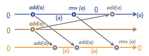
Figure 1: Set with concurrent addition and remove [11]

Thus, a set CRDT has different global post-conditions in order to take into account the concurrent updates while ensuring eventual consistency. Each CRDT has a payload which is an internal data structure not exposed to the client application, and lookup, a function on the payload that returns a set to the client application. For a set CRDT, the pre-conditions must be locally true on the lookup of the set.

Different set CRDTs [11] are the G-Set, 2P-Set, LWW-Set, PN-Set, and OR-Set. They are described below.

1.2 G-Set

In a Grow Only Set (G-Set), elements can only be added and not removed. The CvRDT merge mechanism is a classical set union.

1.3 2P-Set

In a Two Phases Set (2P-Set), an element may be added and removed, but never added again thereafter. The CvRDT 2P-Set (known as U-Set [15]) payload consists in two add-only set $A$ and $R$. Adding an element adds it to $A$ and deleting en elements add it to $R$. The lookup returns the difference $A\setminus R$. The set $R$ is often called the tombstones set.

The CmRDT 2P-Set does not require tombstone but causal delivery; thus, a remove is always received after the addition of the element.

1.4 LWW-Set

In a Last Writer Wins Set (LWW-Set), each element is associated to a timestamp and a visibility flag. A local operation adds the element if not present and updates the timestamp and the visibility flag (true for $add$, false for $rmv$). The CvRDT merge mechanism makes the union of all elements and for each element the pair (timestamp, flag) of the maximum timestamp.

In the CmRDT, the execution of a remote operation updates the element only if timestamp of the operation is higher than the timestamp associated to the element. The both CRDTs requires tombstones and the lookup returns elements which have a true visibility flag.

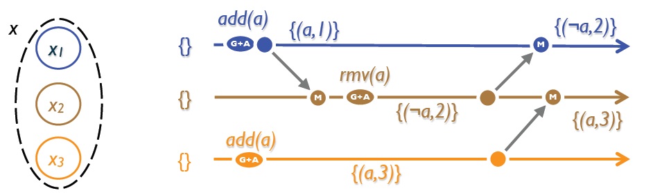
Figure 2: Last Writer Wins Set : LWW-Set [11]

1.5 C-Set

In a Counter Set (C-Set), each element is associated to a counter. Let $k$ be the value of the counter of an element. A local $add$ can occurs only if $k\leq 0$ and sets the counter to $1$ ($\delta=-k+1$). A local $rmv$ can occurs only if $k>0$ and sets the counter to $0$ ($\delta=-k$). The CvRDT (also call PN-Set) payload contains the set of element, and for each element a set $P$ of increments and a set $N$ of decrements. A local $add$, resp. $rmv$, adds $|\delta|$ element in $P$, resp. $N$. The merge operation is the union of the sets. The lookup contains elements with $|P|>|N|$.

In the CmRDT, each operation contains the difference $\delta$ obtained during local execution. The remote operation execution adds $\delta$ to the counter. Element with a counter $k=0$ can be removed, the others must be kept. The lookup contains elements with $k>0$.

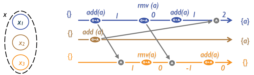
Figure 3: Counter Set : C-Set [11]

1.6 OR-Set

In a Observed Remove Set (OR-Set) each element is associated to a set of unique tag. A local $add$ creates a tag for the element and a local $rmv$ removes all the tag of the element. The CvRDT contains the set of element, and for each element a set $T$ of tags added and a set $R$ of tags removed. The merge operation is the union of each set. The lookup contains elements with $T\cap R\neq\{\}$.

In the CmRDT, each operation contains the tag(s) added or removed. Since causal ordering is ensured and since tag are unique, the removed tag (and element with no tag) can be removed in the payload. The lookup contains the elements of the payload.

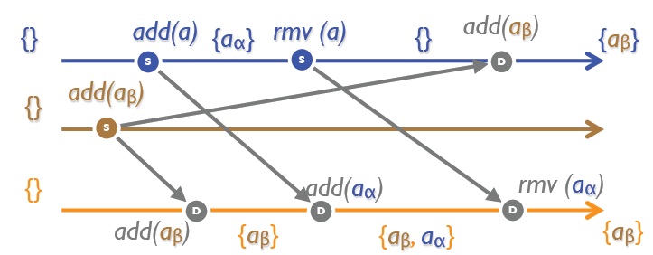
Figure 4: Observed-Remove Set : OR-Set [11]

1.7 Comparison

From the application point of view, all set CRDTs provide a set lookup and the same pre-conditions on operations (except for G-Set, since the application cannot remove an element and for 2P-Set, since application cannot re-add an element). They also provide the same post-conditions of the local replica. The behavior of the presence of the elements in the lookup can be resumed as follow :

LWW-Set

an element appears in the lookup if and only if the operation with the higher timestamp is an $add$.

C-Set

an element appears in the lookup if and only if the sum of the $add$ operations counters is greater than the sum of the $rmv$ operations counters.

OR-Set

an element appears in the lookup if and only if the tags associated by $add$ operations are not all present in $rmv$ operations.

2 Graph Trees

According to standard graph theory definition, a tree – more precisely an arborescence – is a connected directed acyclic graph in which a single node $root$ is designated as the root and there is a unique path from $root$ to any other node [2]. A tree is thus a ordered pair $G=(V,E)$ with $V$ a set of nodes and $E\subseteq V\times V$ a set of directed edges. If $(x,y)\in V$, we say that $y$ is a child of $x$. Since $G$ have no directed cycle, $E^{*}$, the transitive closure of $E$, is a partial strict order on $V$. There is a path from $x$ to $y$ if and only if $(x,y)\in E^{*}$.

We define subtrees in a more general manner than usual by including edges directed to the subtree. In an actual tree there is only one such edge.

Definition 1.

An ordered pair $(N,F)$ is a subtree of the tree $(V,E)$ and is rooted by $n\in N$ if $N\subset V$, $F\subseteq E$ and $(N,F\setminus((V\setminus N)\times N))$ is a connected directed acyclic graph with a unique path from $n$ to any other node and if $(V\setminus N,E\setminus F)$ is a tree.

We consider that the graph can be modified trough two minimal operations $add$ and $rmv$. The operation $add(n,m)$ adds a node $n$ in the graph under the node $m$ and the operation $rmv(N,F)$ removes the set of nodes and edges appearing in a subtree. Other operations, e.g. adding a whole subtree, or removing a node while moving all its children under the father of $n$, can be defined upon these minimal operations. We have the following formal definition of the sequential operations on a tree. For sake of simplicity, we consider that the root of the tree is always present and immutable.

• $pre(add(n,m),(V,E))\equiv n\notin V\wedge m\in V$

• $post(add(n,m),(V,E))\equiv n\in V\wedge(m,n)\in E$

• $pre(rmv(N,F),(V,E))\equiv subtree((N,F),(V,E))$

• $post(rmv(N,F),(V,E))\equiv N\cap V=\{\}\wedge F\cap E=\{\}$.

With such pre- and post-conditions we can ensure that the graph $(V,E)$ stays a tree in case of a sequential modifications. However, in case of a concurrent modifications, these post-conditions conflicts if a node is concurrently added and removed, if a node is concurrently deleted while a children is added, or if a node concurrently added under to different fathers.

2.1 Concurrent addition and deletion of the same element

The post-conditions of $add(n,m)||rmv(N,F)$ with $n\in N$ conflicts, i.e. a node cannot be concurrently added and removed. Indeed, as for a set, the post-condition of $add$ and $rmv$ operations cannot be globally ensured while ensuring convergence.

We can uses sets CRDT to bypass the conflict. By using sets CRDT to handle both sets of nodes and edges, we obtain a data type $(V,E)$ that is obviously eventually consistent. Such trees CRDT have the following behavior.

GG-Tree

In a Grow-only Graph Tree (GG-Tree) nodes and edges can only be added and never removed. A GG-Tree uses G-Sets as the sets of nodes $V$ and edges $E$.

2G-Tree

In a Two-phases Graph Tree (2G-Tree) nodes and thus edges can only be added once. A 2G-Tree uses the lookup of a 2P-set as the set of nodes $V$. There is no need for using set CRDT for the edges since a new edge is only added with a new node. Thus, an edge cannot be added and removed concurrently.

LG-Tree

In a Last-writer-wins Graph Tree (LG-Tree) a node, or a edge, appears in the lookup if and only if the operation with the higher timestamp applied on it is an add. LG-Tree uses the lookup of LWW-element-Sets as the sets of nodes $V$ and edges $E$. The operations become $add(n,m,t)$ and $rmv(N,F,t)$. The execution of the operations consists in updating the timestamp and the visibility flag if the operation timestamp is newer that the attached timestamp.

CG-Tree

An Counter Graph Tree (CG-Tree) a node or a edge appears in the lookup if and only if the sum of $add$ operations applied on it is greater than the sum of $rmv$ operations. A CG-Tree uses the lookup of C-Sets as the sets of nodes $V$ and edges $E$. The operation $add$ and $rmv$ associate an increment to each element appearing in these operation. The execution of the operation applies this positive or negative increment to the targeted elements.

OG-Tree

In an Observed-remove Graph Tree (OG-Tree), a node or a edge appears in the lookup if and only if the tags associated by $add$ operations applied on it are not all removed by $rmv$ operations. An OG-Tree uses the lookup of OR-Sets as the sets of nodes $V$ and edges $E$. The operation $add$ associates a unique tag and $rmv$ associates a set of tag to each element appearing in these operation. The execution of the operation adds or removes the tag(s) to the targeted elements.

2.1.1 Set lookup

From all the above tree CRDTs, we can obtain $(V_{L},E_{L})$ a pair of lookup sets which is eventually consistent since lookup of the set CRDTs is eventually consistent. However, in case of concurrent modifications, this pair $(V_{L},E_{L})$ is not a graph since $E_{L}$ may contain edge on nodes not in $V_{L}$. For instance in the LG-Tree, if the operations $add(n,m,t)$ and $rmv(N,F,t^{\prime})$ with $n\in N$ and $t^{\prime}>t$ are generated concurrently, we get $(m,n)\in E_{L}$ while $n\notin V_{L}$.

The pair $(V_{L},E_{L}\cap(V_{L}\times V_{L}))$ is a graph but may not be a tree. It can be non-connected if a replica adds a node under $m$ and another replica removes $m$ concurrently. Also, there can be several paths between the root and a node since two replicas can add concurrently a node under two different fathers. Moreover, such a graph may contains cycles if, for instance, a replica generates $add(x,root)$ followed by $add(y,x)$ and another replica generates concurrently $add(y,root)$ followed by $add(x,y)$.

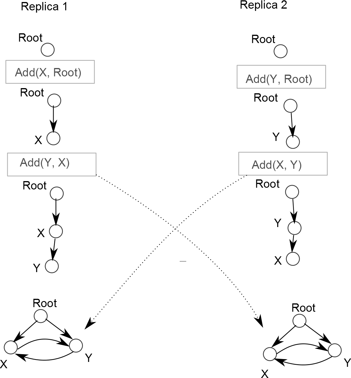
Figure 5: Cycle generated by concurrent additions

We propose to compute a lookup from the pair $(V_{L},E_{L})$ on order to obtain a lookup which is an eventually consistent tree. In the following sections, we propose different policies to firstly reconnect or drop the isolated components to obtain a rooted graph, and to secondly to express a tree from the rooted graph.

2.2 Connection policy

The operations $add(n,m)||rmv(N,F)$ with $m\in N$ and $n\notin N$ conflicts since a naive lookup of the underlying sets CRDTs of nodes and edges is a non connected graph. However, several solutions can be designed to produce a graph which is rooted, i.e. with at least one path from the root to any other node. The solutions can be to “skip” such $add$, to “recreate” the removed ascendant(s), or to place such added nodes “somewhere” in the tree (for instance under the root). We compute a rooted graph $(V_{C},E_{C})$ directly from the lookup $V_{L}$ and $E_{L}$ of the supporting sets CRDTs.

We note $E_{G}=(E_{L}\cap(V_{L}\times V_{L}))$. We call a orphan node, a node $n$ in $V_{L}$ such that $(root,n)\notin E_{G}^{*}$. Since a node is always added with an edge directed to it, an orphan node $n$ has at least one edge in $(m,n)\in E_{L}$ directed to it; if $m\notin V_{L}$, we call $(m,n)$ an orphan edge, elsewhere $m$ and $n$ are parts of the same orphan component.

To compute $(V_{C},E_{C})$, we start by adding all non-orphan nodes and the edges between them in $(V_{L},E_{L})$. Then, we treat the orphan nodes in $V_{L}$. Considering each orphan node $n$, we can apply the following “connection” policies :

skip

drops the orphan node. This algorithm consists simply on a graph traversal starting from the root and is in $\Theta(|E_{L}|+|V_{L}|)$.

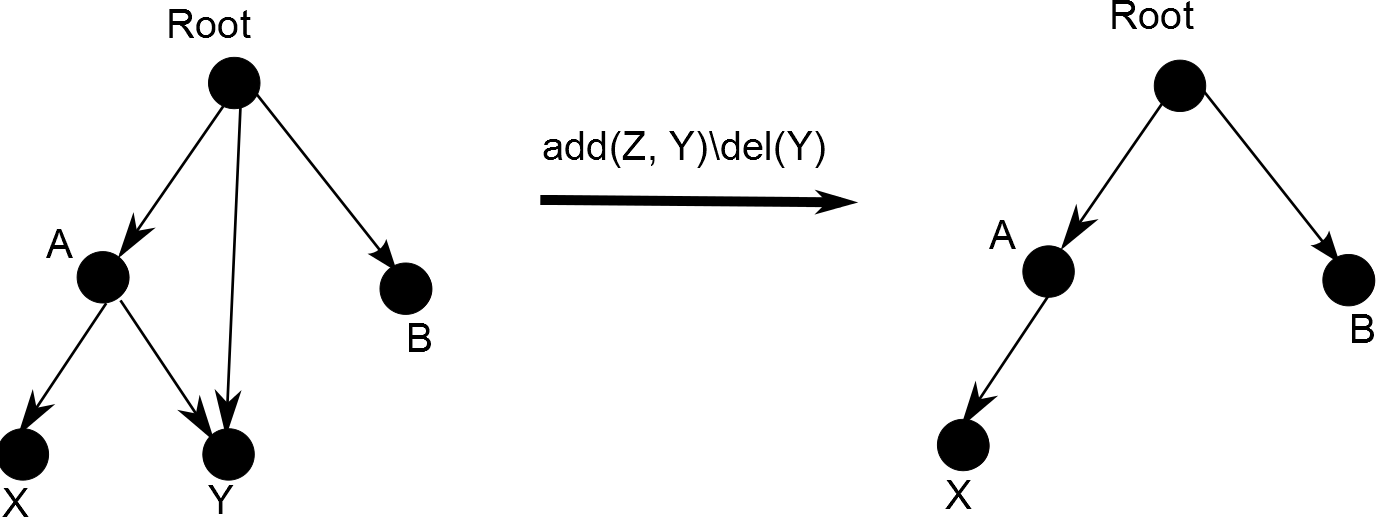
Figure 6: skip policy

reappear

recreates all paths leading to orphans components. We add all edges $(n,y)$ such that $y\in V_{L}$. For each orphan edge $(x,n)$ we add all paths (nodes and edges) that have ever existed between $root$ and $y$. This policy requires to keep as tombstones all the edge ever added to the graph. This algorithm is in $\Theta(|E|+|V|)$.

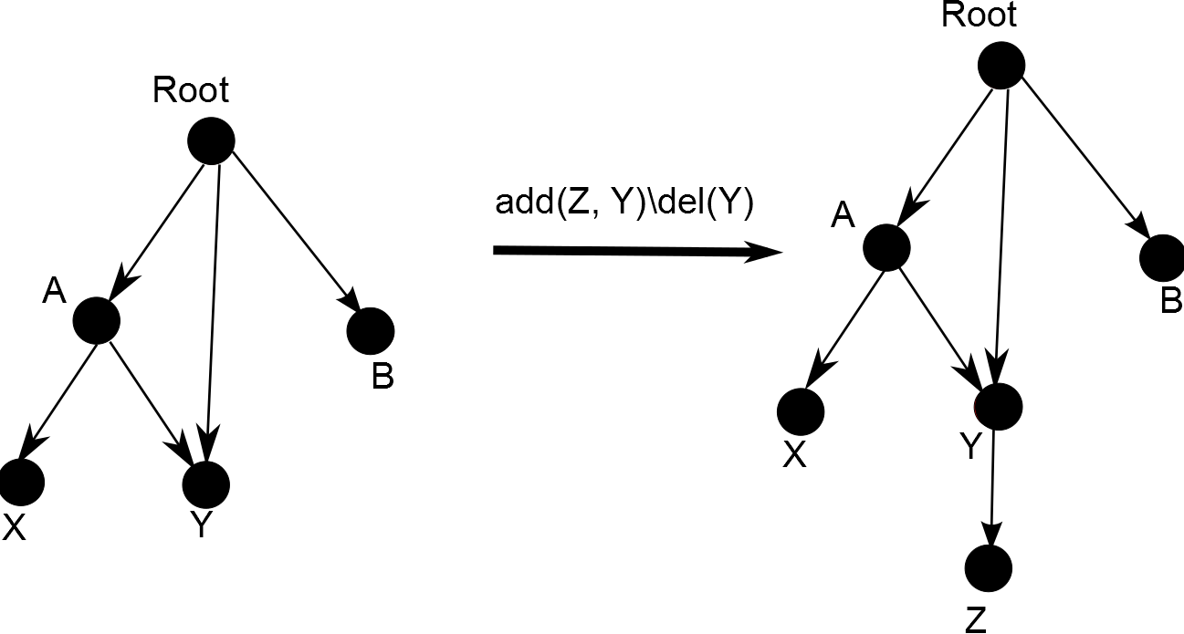
Figure 7: reappear policy

root

places the orphan components under the root. We add all edges $(n,y)$ such that $y\in V_{L}$. For each orphan edge $(x,n)$, we add $(root,n)$. This algorithm consist in modification of all orphans edges : we replace inexistent node by root. This algorithm complexity is $\Theta(|E_{L}|+|V_{L}|)$.

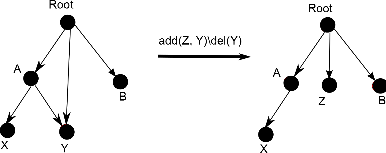
Figure 8: root policy

compact

places the orphan components under the connected node that have ever a path to it. We add all edges $(n,y)$ such that $y\in V_{L}$. For each orphan edge $(x,n)$, we add $(z,n)$ for all $z$ which is a non-orphan node such that a path that does not contains non-orphan nodes have ever existed between $z$ and $x$. This policy requires to keep as tombstones all the edge ever added to the graph. Let $connectSet$ be a set associated on all node. By default this set is empty. We execute the follow algorithm with node previously deleted and connected to orphans edges.

⬇

function getConnected(node n)

if n is not orphan then

return {n}

endif

if n.connectSet is empty then

for n’ in father node

n.connectSet.add(getConnected(n’))

return n.nonnectSet;

else

return n.connectSet

end if

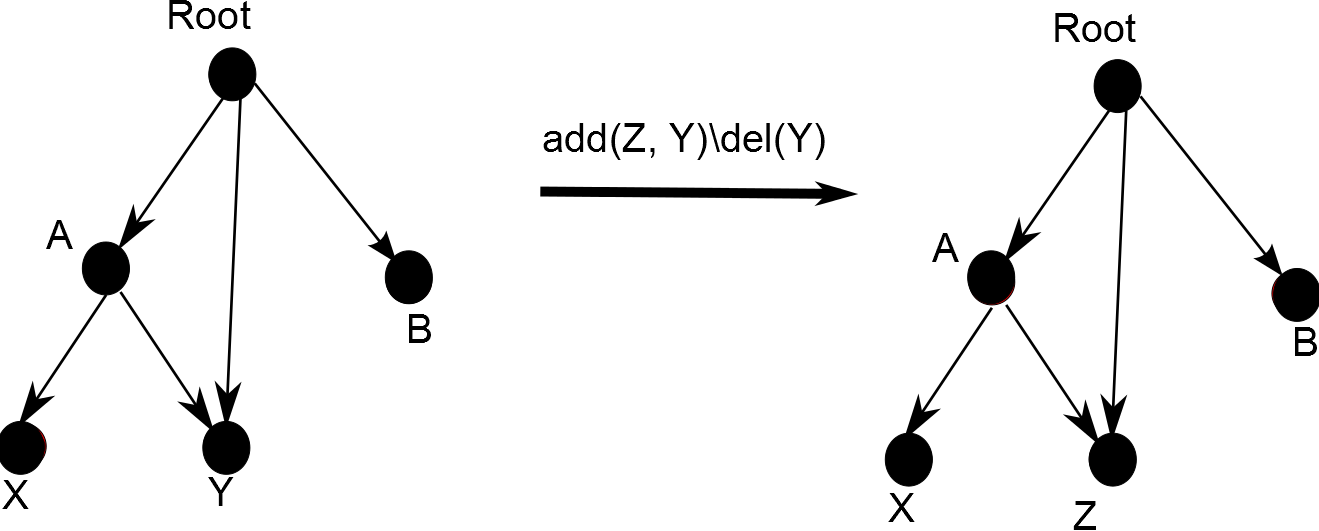
Figure 9: Compact policy

Finally for all orphan edge we add all edges link connected from each element returned by algorithm to the component node.This algorithm is in $\Theta(|E|+|V|)$

Using any of the above policies ensures that $(V_{C},E_{C})$ is a rooted graph for any tree CRDT. Such a graph is eventually consistent and there is at least one path from $root$ to each other node.

The reappear and compact policies require to keep all edges that have ever existed as tombstones. In some set CRDTs approaches (such as CmRDT LWW-Set or all set CvRDTs), these tombstones already exist in the payload. In the compact policy, we can store only the set of node that have ever been accessible from one node.

2.3 Mapping policy

The operations $add(n,m)||add(o,p)$ with $n=o$ and $m\neq k$ conflict. A node cannot be concurrently added under two different nodes, since the graph may contains different paths to a node and directed cycles. To obtain a tree we start from the rooted graph $(V_{C},E_{C})$ and we apply one of the three following “mapping” policies.

several

: We construct all the acyclic paths in the graph. Thus, copies of the node can appear in different places in the tree. Remove a copy of the node removes all the others. The algorithm is a simple depth-first that begins on root node. For each node, the algorithm is

1. Mark the node.

2. Construct a list $l$ composed of recursive calls on all unmarked children nodes.

3. Unmark the node.

4. Returns a tree composed of the node and the list $l$ of children

Obtaining a description of all simple paths in a directed graph can be computed using $O(|V|^{3})$ matrix operations. Such a tree contains up to $|V|!$ edges in case of a complete graph.

one

: This policy adds in the tree each node in $V_{L}$ only once. Thus, the algorithm must make a choice on the edges :

newer

: The “newer” variation needs a timestamps on edges to select the newer. This is adapted to LG-Tree that already has such timestamp. We construct a Maximal Spanning Tree (MST) with the edges sorted by timestamp. We will not obtain a tree composed with only newest edges since such edges may constitute a cycle. But we will obtain a tree with the maximal sum of timestamp. This tree will be rooted since $root$ has no edge directed to it and must be included in the MST. Building a MST in a directed graph can be achieved in $\Theta(|E|+|V|log|V|)$ [3].

higher

: This variation is designed for CG-Tree and OG-Tree. We construct a MST maximising edges counters or edge tags numbers.

shortest

: This variation can be used for all type of tree. For each node we select the shortest path to it. A Breath-first algorithm can be used to produce the tree in $\Theta(|E|+|V|)$.

zero

: The zero policy removes all subtrees rooted by nodes which have more than one edge directed to them. For each node the algorithm checks the number of input edges. The algorithm traverses the graph starting from the root but does not add nodes with an in degree greater than two and does not visit its children. The algorithm is in $\Theta(|V|+|E|)$.

2.4 Discussion on graph trees

Thus, we can obtain a lookup using a graph structure managed by set CRDTs. This lookup function is composed in three phases. The first phase is the lookup of the underlying set CRDT. The second phase computes a rooted graph. The third phase expresses a tree from the rooted graph. Such data types are obviously CRDTs since the underlying sets are eventually consistent, and since the lookup tree is computed with deterministic policies, this lookup is also eventually consistent.

However, depending on the policy chosen, the client application can observe moves on the lookup tree. For instance, using a root policy, if a removed father is added again, its orphan son will move from the root to its original place.

We call monotonic policy, a policy where $add$ and $rmv$ operations do not move an existing node in the lookup. The non-monotonic policies are : root, compact and all one variations. The monotonic policies are skip, reappear, zero and several.

The lookup function works after each modification of the tree. The complexity of this function could be up to factorial for the several policy. So, some optimizations are useful. We call incremental lookup function, a lookup function which reuses an previous calculus to avoid recompute entire tree. For example, in the reappear policy, when an orphan node should be added, the incremental lookup function adds to the tree the several/one/zero paths leading to this node. On the other hand, when the father of an orphan node is added, the other reappeared paths must be removed of the lookup. Finally, when an orphan node is removed, the reappeared paths should disappear. Such incremental versions have the same worst-case complexity than non-incremental ones but are slightly more efficient. However, eventual consistency of the lookup is less straightforward to ensure in such incremental versions.

2.5 A special case : 2G-Tree

A two phases graph tree (2G-Tree) uses a 2P-set [11] as the set of nodes $V$. A 2P-Set consists in defining unique elements that can only be added once on all replicas. Thus, node and edge cannot be added and removed concurrently. The other main advantage of the 2G-Tree is that the conflict $add||add$ does not occurs since a node can only be added once. Thus, 2G-Tree do not require any mapping policy.

In a 2G-Tree, the conflict $add(n,m)||rmv(N,F)$ with $m\in N$ and $n\notin N$ can be resolved using solutions presented above. Assuming that node can be found in constant time (using hash table), the skip policy can be computed incrementally in $\Theta(1)$ time. Indeed, the remove of a node consists in remove of the entire subtree, and addition of an orphan node has no effect. Moreover a CvRDT 2G-Tree can send constant size messages for remove : $rmv(n)$ with $n$ the root of the subtree. The reappear and compact policy can be computed in $\Theta(|V|)$ since there is only one path, of size at most $|V|$, leading to a given node. Finally, in the root policy, the addition of a node is always in $\Theta(1)$ time.

2.6 EDGE trees

Since a node is always added with an edge directed to it, one can represent a tree using only edges. Such a choice leads to a data structure we call edge tree. Given a finite or infinite set of nodes $V$, an edge tree is a subset of all ordered pairs. An edge tree has a root with no edge directed to it, and for all edge, it exists one unique parent edge. A subtree is rooted by a node and include the edge directed to this node and a set of connected edges.

Definition 2.

An edge tree $T$ rooted by $root$ is a subset of $V\times V$ such that for all $(x,y)\in T$ either $x=root$, or there exists a unique $z\in V$ such that $(z,x)\in T$.

The set $S$ is a subtree rooted by $n\in V$ of $T$ if $S\subset T$, $\exists(x,n)\in S$, $\forall(a,b)\in S.~{}b\neq n\implies(n,b)\in S^{*}$ and $T\setminus S$ is an edge tree.

We have the following formal definition of the sequential operations on an edge tree.

• $pre(add(n,m),T)\equiv\exists(z,m)\in T$

• $post(add(n,m),T)\equiv(m,n)\in T$

• $pre(rmv(S),T)\equiv subtree(S,T)$

• $post(rmv(S),T)\equiv S\cap T=\{\}$.

As for graph tree, the post-conditions of $add$ and $rmv$ conflict and an edge tree CRDT uses a set CRDT to handle the set of edges. We can apply the same connecting and mapping policies than for graph tree to compute a tree lookup of the CRDT set. We simply consider that a node belong to a tree if and only if it appears on an edge of tree.

Such GE-Tree, 2E-Tree or OE-Tree will have exactly the same behavior than respectively GG-Tree, 2G-Tree and OG-Tree. Indeed, in such trees, we cannot remove edges (GG-Tree), or we cannot have an edge directed to a removed node (2G-Tree and OG-Tree). Thus, GE-Tree, 2E-Tree and OE-Tree are optimizations of their respective xG-Tree.

The LE-Tree and CE-Tree have a different behavior than LG-Tree and CG-Tree. Indeed, let consider a first replica that inserts a node $x$ under a node $y$, and then removes $x$, while a second replica insert $x$ under a node $z$. Depending on the timestamps (LG-Tree) or on if another replica removes $(y,x)$ concurrently (CN-Tree), the node $x$ – and thus $(z,x)$ – can appear or not in the lookup. In LE-Tree and CE-Tree, $(z,x)$ appears in the lookup.

3 Word trees

In this section we introduce word trees, another data structure to manage concurrently modified trees. A word represents a path in the tree, a tree can be defined as a set of words : the set of paths existing in this tree. We use the standard definitions about words. Let $\Sigma$ be a finite – or infinite – ordered alphabet, a word is a finite sequence of elements from $\Sigma$. The length of a word $w$, noted $|w|$ is the number of elements of $w$. We denotes $\varepsilon$ the empty word. The concatenation $vw$ is the word formed by the joining end-to-end the words $v$ and $w$. The set of all strings over $\Sigma$ of any length is the Kleene closure of $\Sigma$ and is denoted $\Sigma^{*}$.

We define a tree as a set of the words representing all the paths in the tree. Since all the paths are present in the set, any prefix of a path is also a path of the tree. The empty word $\varepsilon$ is the root of the tree.

Definition 3.

A word tree $T$ is a subset of $\Sigma^{*}$, such that $\varepsilon\in T$ and $\forall p,e\in\Sigma^{*}.~{}pe\in T\implies p\in T$.

A subtree is defined as complete set of paths with a common prefix.

Definition 4.

In a tree $T$, a subtree $P$ is a subset of $T$ such that $T\setminus P$ is a tree and such that $\exists w\in T.~{}\exists S\subset\Sigma^{*}.~{}P=\{ws|s\in S\}$ and $S$ is a tree.

As for graph tree, there is two operations to modify a word tree. The operation $add(n,p)$ with $n\in\Sigma$ and $p\in\Sigma^{*}$ adds a new path and $rmv(P)$ removes the set of paths representing a subtree.

• $pre(add(n,p),T)\equiv p\in T\wedge pn\notin T$

• $post(add(n,p),T)\equiv pn\in T$

• $pre(rmv(P),T)\equiv P\subset T\wedge subtree(P,T)$

• $post(rmv(P),T)\equiv P\cap T=\{\}$

With such pre- and post-conditions, we can ensure that the set $T$ is sill a tree in case of sequential modifications. In case of concurrent modifications, word trees differ from graph trees since only $add||del$ conflicts occurs.

3.1 Concurrent addition and remove of the same element

A for mathematical set, the post-conditions of $add(n,p)$ and $rmv(P)$ with $np\in P$ conflicts since convergence cannot be achieved. As for graph trees, we can use set CRDT to bypass the conflict. The obtained tree CRDT have the following behavior :

GW-Tree

a path can only be added and never removed.

2W-Tree

a path can only be added once. Such a CRDT has the same behavior than the 2G-Tree and 2E-Tree.

LW-Tree

a path appears in the lookup if and only if the operation with the higher timestamp applied on it is an $add$.

CW-Tree

a path appears in the lookup if and only if the number of $add$ operations applied on it is greater than the number of $rmv$ operations.

OW-Tree

a path appears in the lookup if and only if the tags associated by $add$ operations applied on it are not all removed by $rmv$ operations.

All the above data types are obviously eventually consistent. But the lookup presented must be a tree even in case of the concurrent addition of a node and remove of its father.

3.2 Concurrent addition of a path and remove of the prefix

As for graph and edge trees, the naive execution of operations $add(n,p)$ and $rmv(P)$ with $p\in P$ produce a set of path which is no longer a tree. Thus we need to compute a lookup which is a tree. We compute a lookup tree $LT$ from the set of path $LS$ obtained from the lookup of the supporting set CRDT.

We call a orphan path, a path in $LS$ that has a prefix which is not in $LS$. We start by adding all non-orphan paths of $LS$ to $LT$. Then, we treat the orphan paths in $LS$ in length order (shortest first, then $\Sigma$ order). Considering each orphan path $a_{1}a_{2}\ldots a_{n}\in LS$ with $\forall i\in[1,n].~{}a_{i}\in\Sigma$, we can apply the following connection policies :

skip

drops the orphan path.

reappear

recreates the path leading to the orphan path. We add all $a_{1}\ldots a_{j}$ with $j\in[1,n]$.

root

places the orphan subtree under the root. We add $a_{j}\ldots a_{n}$ to $LT$ with $j$ such that $a_{1}\ldots a_{j-1}\notin LS$ and $\forall k\in[j,n]$, $a_{1}\ldots a_{k}\in LS$.

compact

places the orphan subtree under its longest non-orphan prefix. We add $a_{1}\ldots a_{m}a_{j}\ldots a_{n}$ to $LT$ with $j$ and $m$ such that $m<j$ and $a_{1}\ldots a_{m}\in LT$ and $a_{1}\ldots a_{m+1}\notin LS$ and $a_{1}\ldots a_{j-1}\notin LS$ and $\forall k\in[j,n]$, $a_{1}\ldots a_{k}\in LS$.

Example 1.

For a lookup $LS=\{\varepsilon,a,ab,ac,abcd,abcde,abcdefg\}$, the orphans path are $\{abcd,abcde,abcdefg\}$ and we obtain $LT$ equal to :

skip

$\{\varepsilon,a,ab,ac\}$

reappear

$\{\varepsilon,a,ab,ac,abc,abcd,abcde,abcef,abcdefg\}$

root

$\{\varepsilon,a,ab,ac,d,de,g\}$

compact

$\{\varepsilon,a,ab,ac,abd,abde,abdeg\}$

Using any of the above policies ensures that the lookup trees presented to the client by any CRDT tree are eventually consistent.

Theorem 1.

The lookup sets $LT$ computed using a skip, root, reappear, or compact policy are tree and are eventually consistent.

Proof.

Since the set of paths $LS$ is eventually consistent, and since the paths are treated is the same order and since each policy is deterministic, the computed set of paths $LT$ is eventually consistent.

Set of path $LT$ is a tree since :

skip

there is no orphan path in $LT$.

reappear

we add an orphan path in $LT$ with all its prefixes.

root

a suffix $a_{j}\ldots a_{n}$ is added to $LT$ only if $\forall k\in[j,n]$, $a_{1}\ldots a_{k}\in LS$. Thus, all the prefixes $a_{j}\ldots a_{k}$ were also added to $LT$.

compact

a path $a_{1}\ldots a_{m}a_{j}\ldots a_{n}$ is added to $LT$ only if $\forall k\in[j,n]$, $a_{1}\ldots a_{k}\in LS$. Thus all the prefixes $a_{1}\ldots a_{m}a_{j}\ldots a_{k}$ were also added to $LT$.

∎

Computing a lookup tree $LT$ every time the lookup set $LS$ is modified ensures easily eventual consistency, but only some policies are monotonic. We consider a policy as monotonic if the $add(p)$ operation do not moves any already existing node in tree. The root and compact policies are not monotonic since when the missing ascendants are added again, the orphan subtree moves to its original place.

The advantage of monotonic policies is that the client of the tree CRDT will not observe such move, and that a client operation on an orphan path do not require a complex translation into an operation on the supporting set CRDT.

3.3 Complexity and optimisation

Lets assume that a hash table is used to implement the set of paths. Thus, checking for all prefixes of path if they belongs to a set have an average time complexity proportional to the length of the path. Thus, the time complexity to apply a policy to a path is linear. Also, the time complexity to compute a lookup tree is $\Theta(pk)$ in average, with $p$ the number of paths in $LS$ and $k$ the average length of these paths. The worst case time complexity is $\Theta(n^{2})$ with $n$ the number of paths in $T$.

However, at least for the monotonic policies, we can compute $LT$ incrementally, i.e. without parsing the whole set $LS$.

skip

When an orphan path is supposed to be added in the lookup, we drop it. When an non-orphan path $p$ is added, we add recursively all $pa\in LS$ with $a\in\Sigma$. When a path $n$ is supposed to be removed in the lookup, we remove all the paths that are prefixed by $n$. Moreover, a tree CmRDT can send only the operation $rmv(n)$ with $n$ the common prefix of the subtree, since the whole subtree will be removed.

reappear

In the reappear policy, when an orphan path is removed we must remove the reappeared path to ensure eventual consistency. This can be done by marking the reappeared paths as “ghosts”. When path previously marked as ghost is supposed to be added in the lookup, we unmark it. When an orphan path $n$ is supposed to be added in the lookup, we add all the prefixes of $n$ that are not existing and we mark them as ghost. When a path $n$ is supposed to be removed in the lookup, if $n$ is the prefix of a non-ghost path, we mark $n$ as ghost, elsewhere we remove $n$ and all the ghost prefixes of $n$ that are the prefixes of not any ghost.

4 Ordered trees

In this section, we present ordered trees, where the set of children of a node is totally ordered. For this we need to add to the unordered trees presented above, an additional information called Position Identifier (PI) which allows to order the children. These position identifiers must be totally ordered to ensure eventual consistency and defined within a dense space to allow insertion of a node at an arbitrary position. These position identifiers can be associated to nodes or edges.

To obtain position identifiers, an idea to use PI already defined for sequence editing CRDTs such as Logoot [14], Woot [8], WOOTO [13], RGA [10] or Treedoc [9]. Such PIs are Unique Position Identifier (UPI) and thus constrain the behavior of the trees to some kind of two-phases set that does not allow concurrent insertions of the same element or re-insertions. So, we propose a new non-unique position identifier to allow such operations.

In the following figures, a plain arrow represents the child relation between node, and a dotted arrow represents the order between children.

4.1 Unique positioning for nodes

We associate each node to an unique position identifier (UPI). The order between the children of a node is given by their UPI. Since only graph trees manage nodes and since position identifiers are unique, we obtain a 2G-Tree. If a node is added twice concurrently, even at the same place in the ordered tree, we obtain two different nodes. The formal definition of the operation $rmv$ do not change, a node is a pair $(element,UPI)$ and an edge is a pair of node. The formal definition of operation add becomes :

• $pre(add((n,u),(m,v)),(V,E))\equiv(n,u)\notin V\wedge(m,v)\in V\wedge unique(u)$

• $post(add((n,u),(m,v)),(V,E))\equiv(n,u)\in V\wedge((m,v),(n,u))\in E$

The conflict $add||add$ does not occurs, since a node can only be added once with an UPI. In figure 10, a replica produces $add(Z,A)$ while another replica produces $add(Z^{\prime},B)$ concurrently, but they are considered as two different elements with same characteristics.

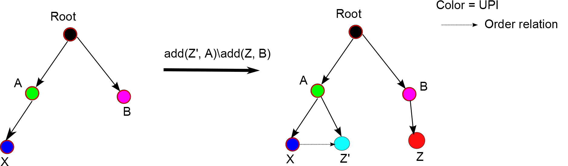
Figure 10: Concurrent operations add/add with node positioning

The conflict $add(n,m)||rmv(N,F)$ with $m\in N$ and $n\notin N$ can be resolved with the same policies defined for 2G-Tree in Section 2.5. In figure 11, we represent the execution of two concurrent operations $add(Z,Y)/rmv(Y)$ with the skip policy.

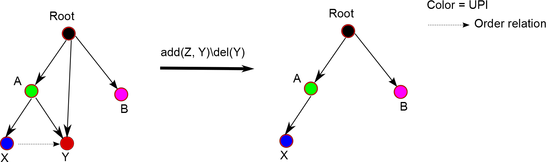
Figure 11: concurrent operations add/del with skip policy

A tree with UPI associated to nodes can be built using any sequential editing UPIs. However the WOOT and RGA UPI requires tombstones and thus are more adapted to a 2P CvRDT that contains these tombstones. For 2P CmRDT, the Logoot or Treedoc UPI approaches are more suitable. The complexity of the children order computation depends on the approach used. An example of such construct is [6].

4.2 Unique positioning for Edges

To allow concurrent insertions on the same node at two different places in the tree or to build edge or word tree, we propose to associate UPI to edges. The order between the children of a node is given by the UPI of the outgoing edge. In graph and edge trees an edge becomes a triple $(m,n,u)$ with $m$ and $n$ two nodes and $u$ an UPI. In word trees, a path becomes $u_{1}a_{1}u_{2}a_{2}u_{2}\ldots u_{n}a_{n}$ with $a_{i}$ elements of $\Sigma$ and $u_{i}$ UPIs. The difference between ordered trees with edge positioning and node positioning is illustrated in figures 12 and 10.

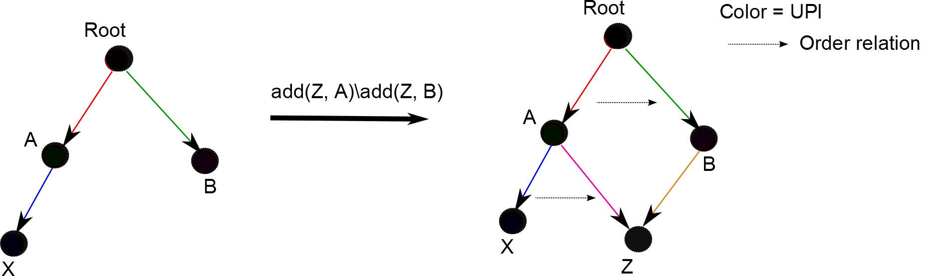
Figure 12: Concurrent operations add/add with edge positioning

The formal definition of operation $rmv$ does not change and the definition of $add$ becomes :

Graph Tree

• $pre(add(n,m,u),(V,E))\equiv n\notin V\wedge m\in V\wedge unique(u)$

• $post(add(n,m,u),(V,E))\equiv n\in V\wedge(m,n,u)\in E$

Edge Tree

• $pre(add(n,m,u),E)\equiv\exists(z,m,v)\in E\wedge unique(u)$

• $post(add(n,m,u),E)\equiv(m,n,u)\in E$

Word Tree

• $pre(add(n,p,u),T)\equiv p\in T\wedge pun\notin T\wedge unique(u)$

• $post(add(n,p,u),T)\equiv pun\in T$

Such an edge tree is a 2E-Tree since an edge can only be added once. And such a word tree is a 2W-Tree since a path can only be added once. For graph tree, we can manage node using any set CRDT to obtain GG-Tree, 2G-Tree, LG-Tree, CG-Tree or OG-Tree. As for nodes UPI, any sequential editing UPI can be chosen, but these are more or less adapted to the underlying set CRDT. Logoot and Treedoc without tombstones are more appropriate to 2x and OG CmRDT. While WOOT and RGA are more appropriate to LG-Tree, CG-Tree and all CvRDT,

As for unordered trees, the conflicts between addition of a node and remove of its father can be resolved using any connection policy. Conflicts between two concurrent additions of the same element in graph trees can be resolved using any mapping policy.

In graph tree with edge positioning, two concurrent insertion of a node at the same place (same father and same order between children) generates two edges (see Figure 13). In edge tree (and word tree), using a unique position identifier enforces to generate two instances of the edge (and path in word tree). To allow a different behavior, the position identifier must be non-unique.

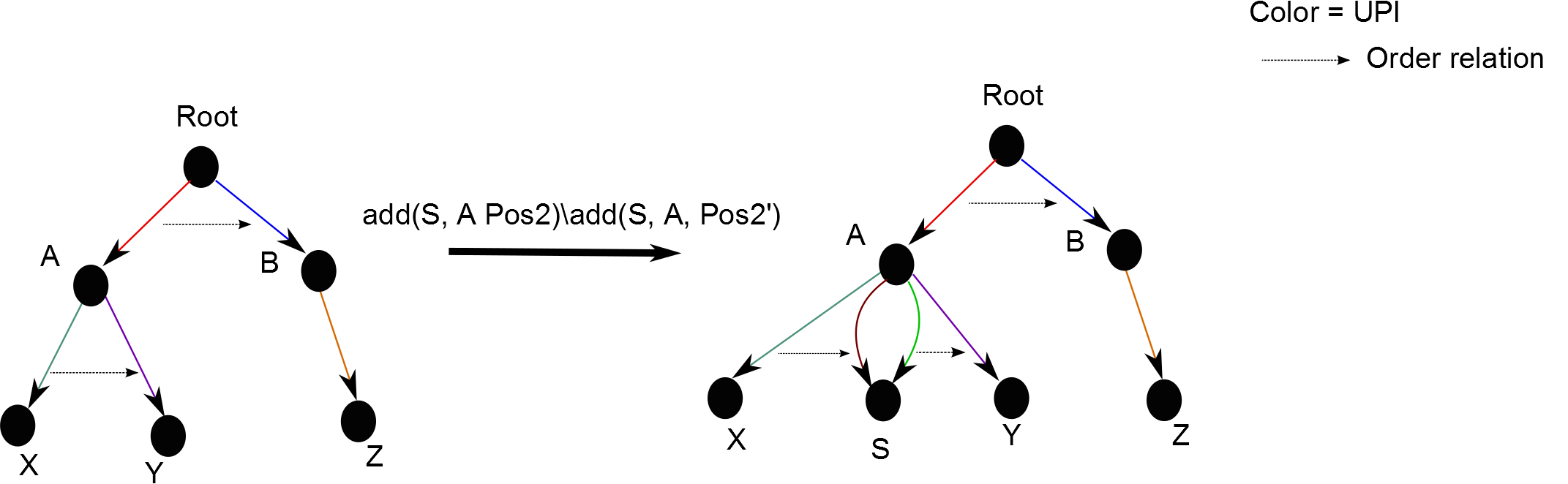
Figure 13: Two concurrent insertions at the same place with edge positioning

4.3 A new sequence editing CRDT : WOOTR

Non-unique position identifiers must be totally ordered and defined within a dense space. To obtain such properties we define a new sequential editing CRDT called Recursive-WOOT (WOOTR).

WOOTR elements are defined inductively upon an alphabet $\Sigma$ (or set of node).

• $\vdash$ and $\dashv$ are elements

• a triple $\langle a,e,f\rangle$ is an element if $a\in\Sigma$ and $e$ and $f$ are elements.

The elements $\vdash$ and $\dashv$ mark respectively the begin and the end of a sequence. When a character $a$ is inserted between two elements $p$ and $n$, we add the element $\langle a,p,n\rangle$. We call $p$ the previous element and $n$ the next element of this new element. The set of the WOOTR elements constitutes the characters present in the sequence. The elements are ordered using the WOOT algorithm [8] assuming that elements with the same previous and next elements are ordered using their character. For instance, starting from an empty sequence, if a replica inserts $a$, followed by $b$, while another replica inserts $c$ concurrently, we obtain the set $\{\langle a,\vdash,\dashv\rangle,\langle b,\langle a,\vdash,\dashv\rangle,\dashv\rangle,\langle c,\vdash,\dashv\rangle\}$ and the sequence is $abc$.

Since elements are not unique, they can be inserted concurrently by two different replicas. However, they can also be added and removed concurrently. Thus, as in any set, we need to manage these concurrent operations. Eventual consistency can be achieved using a set CRDT such as LWW-Set, CG-Set or OR-Set. Contrary to the original WOOT, we do not require to keep deleted elements as tombstones since, when a remote insertion occurs, the WOOT algorithm can find the place of the deleted previous or next element before inserting the element itself. This is particularly suitable for CmRDT OR-Set and C-Set that do not keep all tombstones.

The size of WOOTR elements can be proportional to the size of the document. Due to this size, such a sequential editing CRDT may not be adapted to realtime collaborative text editing [1]. However, we think that it can be useful for trees, since in tree the element are distributed under different fathers, the WOOTR elements grow more slowly.

4.4 Non-unique position identifier

With non-unique position identifiers, only one edge (or path) will be present in the tree in case of concurrent insertion of an element at the same place in the tree. A non-unique position identifier can be used to order any variation of graph, edge or word tree.

For instance, the WOOTR identifier can be added to edge in graph or edge trees. Such edges are ordered pair $(x,w)$ with the $x$ the father node and $w$ a WOOTR element defined on the set of nodes. In word tree, a path becomes $w_{1}\ldots w_{n}$ a string of WOOTR elements defined on the alphabet.

5 Conclusion

In this report, we have proposed several tree conflict-free replicated data types (CRDT). These data types are based on set CRDTs. As any CDRTs, tree CRDTs are eventually consistent and converge without requiring any synchronization.

The unordered tree data types are constructed using a tree representation (graph, edge or word), a set CRDT, one connection policy and one mapping policy (for graph and edge tree). Every combination of choices is possible and is a tree CRDT. Each of the choice correspond to the desired semantic to resolve the two or three different conflicts between operations. The choice of the set CRDT defines the semantic of the concurrent addition and remove of an element. The choice of the connection policy defines the semantic of concurrent remove of an element and addition of a child. The choice of the mapping policy, if required, defines the semantic of the concurrent additions of an element. With such a construct we give to the application programmer the entire control of the behavior of the tree CRDT.

The policies designed make some arbitrary choices to resolve the conflicts. We think that arbitrary choices are mandatory to ensure scalability in large-scale system. However, the application may have a particular semantic on nodes or operations, or the final user may be required to resolve the conflict. To facilitate such mechanism, we can adapt the root policy and the zero policy. We can adapt the root policy to place orphan elements under a special “lost-and-found” node and the zero policy to present to the application the conflicting nodes and edge separately from the tree.

The ordered tree data types are constructed upon unordered trees CRDT. They consist in associating a totally ordered position identifier to elements of the tree. These position identifier comes from existing sequence editing CRDT and ensure eventual consistency without synchronisation. Ordered trees share the same behavior than the corresponding unordered tree except that a tree node can be add at different positions under another node. The choice between the kinds of position identifiers is a question of performance and adaptability with the underlying set CRDT. Moreover, we introduce a new sequence editing CRDT called WOOTR. This sequence editing CRDT is the first to allow reintroduction of an element and to consider that concurrent insertion of an element at the same position is the same operation.

All the combination presented can be used for any application that require a tree. However, we think that some combination are more adapted to some application context. For instance the unordered graph trees are more adapted to applications managing a composite pattern or a file system data structure. Indeed, in Unix-like files system, the hard links allow to place a file or a repository in several different repositories. One another hand, ordered word trees seems more adapted to collaborative editing of structured documents [7].

Finally, some constructs, especially trees builds on 2P-Set, are very efficient, other variations and some policies, especially the several policy in graph and edge trees, are quite costly in term of computation complexity. We need to establish the actual scalability of the constructs trough experimentation on realistic data set since the actual computation cost depends highly on the degree of concurrency.

References

- [1] M. Ahmed-Nacer, C.-L. Ignat, G. Oster, H.-G. Roh, and P. Urso. Evaluating crdts for real-time document editing. In ACM, editor, ACM Symposium on Document Engineering, page 10 pages, San Francisco, CA, USA, september 2011.
- [2] R. Diestel. Graph Theory. Springer-Verlag, fourth edition edition, 2010.
- [3] H. Gabow, Z. Galil, T. Spencer, and R. Tarjan. Efficient algorithms for finding minimum spanning trees in undirected and directed graphs. Combinatorica, 6:109–122, 1986. 10.1007/BF02579168.
- [4] S. Gilbert and N. Lynch. Brewer’s conjecture and the feasibility of consistent, available, partition-tolerant web services. SIGACT News, 33:51–59, June 2002.
- [5] L. Lamport. Time, clocks, and the ordering of events in a distributed system. Commun. ACM, 21(7):558–565, 1978.
- [6] S. Martin and D. Lugiez. Collaborative peer to peer edition: Avoiding conflicts is better than solving conflicts. In H. Weghorn and P. T. Isaías, editors, IADIS AC (2), pages 124–128. IADIS Press, 2009.
- [7] S. Martin, P. Urso, and S. Weiss. Scalable xml collaborative editing with undo. In R. Meersman, T. Dillon, and P. Herrero, editors, On the Move to Meaningful Internet Systems: OTM 2010, volume 6426 of Lecture Notes in Computer Science, pages 507–514. Springer, 2010.
- [8] G. Oster, P. Urso, P. Molli, and A. Imine. Data Consistency for P2P Collaborative Editing. In Proceedings of the ACM Conference on Computer-Supported Cooperative Work - CSCW 2006, pages 259–267, Banff, Alberta, Canada, nov 2006. ACM Press.
- [9] N. M. Preguiça, J. M. Marquès, M. Shapiro, and M. Letia. A commutative replicated data type for cooperative editing. In ICDCS, pages 395–403. IEEE Computer Society, 2009.
- [10] H.-G. Roh, M. Jeon, J.-S. Kim, and J. Lee. Replicated abstract data types: Building blocks for collaborative applications. Journal of Parallel and Distributed Computing, 71(3):354 – 368, 2011.
- [11] M. Shapiro, N. Preguiça, C. Baquero, and M. Zawirski. A comprehensive study of Convergent and Commutative Replicated Data Types. Research Report RR-7506, INRIA, January 2011.
- [12] M. Shapiro, N. Preguiça, C. Baquero, and M. Zawirski. Conflict-free replicated data types. In X. Défago, F. Petit, and V. Villain, editors, Stabilization, Safety, and Security of Distributed Systems (SSS), volume 6976, pages 386–400, Grenoble, France, October 2011.
- [13] S. Weiss, P. Urso, and P. Molli. Wooki: a P2P Wiki-based Collaborative Writing Tool. In Web Information Systems Engineering, pages 503–512, Nancy, France, December 2007. Springer.
- [14] S. Weiss, P. Urso, and P. Molli. Logoot-undo: Distributed collaborative editing system on p2p networks. IEEE Transactions on Parallel and Distributed Systems, 21:1162–1174, 2010.
- [15] G. T. Wuu and A. J. Bernstein. Efficient solutions to the replicated log and dictionary problems. In Proceedings of the third annual ACM symposium on Principles of distributed computing, PODC ’84, pages 233–242, New York, NY, USA, 1984. ACM.