Quantum Spin Pumping Mediated by Magnon

Abstract

We theoretically propose quantum spin pumping mediated by magnons, under a time-dependent transverse magnetic field, at the interface between a ferromagnetic insulator and a non-magnetic metal. The generation of a spin current under a thermal equilibrium condition is discussed by calculating the spin relaxation torque, which breaks the spin conservation law for conduction electrons and operates the coherent magnon state. Localized spins lose spin angular momentum by emitting magnons and conduction electrons flip from down to up by absorbing the momentum. The spin relaxation torque has a resonance structure as a function of the angular frequency of the applied transverse field. This fact is useful to enhance the spin pumping effect induced by quantum fluctuations. We also discuss the distinction between our quantum spin pumping theory and the one proposed by Tserkovnyak et al.

1 Introduction

A new branch of physics called spintronics has seen a rapid development over the last decades. The central theme is the active manipulation of spin degrees of freedom as well as charge ones of electrons; spintronics avoids the dissipation from Joule heating by replacing charge currents with spin currents. Thus establishing methods for the generation of a spin current is significant from viewpoints of fundamental science and potential applications to green information and communication technologies.[1]

A standard way to generate a (pure) spin current is the spin pumping effect at the interface between a ferromagnetic material and a non-magnetic metal. There the precession of the magnetization induces a spin current pumped into a non-magnetic metal, which is proportional to the rate of precession of the magnetic moment. The precessing ferromagnet acts as a source of spin angular momentum; spin battery. This method has been developed by Tserkovnyak et al.[2] Now their formula has been widely used for interpreting vast experimental results, despite the phenomenological treatment of spin-flip scattering processes.

Thus we reformulate the spin pumping theory, through the Schwinger-Keldysh formalism, to explicitly describe the spin-flip processes. A generation of the pumped spin current is discussed on the basis of the spin continuity equation for conduction electrons. Moreover the utilization of magnons, which are the quantized collective motions of localized spins, has recently been attracting considerable interest.[3, 4, 27] Hence, the focus of the present work lies also on the contribution of magnons to spin pumping. We treat localized spins as not classical variables but magnon degrees of freedom. Therefore we can capture the (non-equilibrium) spin-flip dynamics, where spin angular momentum is exchanged between conduction electrons and localized spins, on the basis of the rigorous quantum mechanical theory. Consequently, we can reveal the significance of time-dependent transverse magnetic fields, which act as quantum fluctuations, for the spin pumping effect.

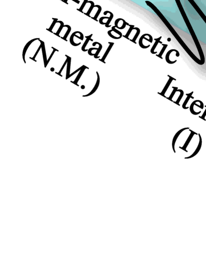
Figure 1: (Color online) A schematic picture of quantum spin pumping mediated by magnons. Spheres represent magnons and those with arrows are conduction electrons. (a) Localized spins lose spin angular momentum by emitting magnons and conduction electrons flip from down to up by absorbing the momentum. (b) An enlarged schematic picture of the interface. The interface is defined as an effective area where the Fermi gas (conduction electrons) and the Bose gas (magnons) coexist to interact; $J\not=0$. Conduction electrons cannot enter the ferromagnet, which is an insulator.

We consider a ferromagnetic insulator and non-magnetic metal junction[3] shown in Fig. 1 where conduction electrons couple with localized spins ${\mathbf{S}}({\mathbf{x}},t)$, ${\mathbf{x}}=(x,y,z)\in{\mathbf{R}}^{3}$, at the interface;

$${\cal{H}}_{\rm{ex}}=-2Ja_{0}^{3}{\int_{{\mathbf{x}}\in\text{(interface)}}}d{\mathbf{x}}{\ }{\mathbf{S}}({\mathbf{x}},t)\cdot{\mathbf{s}}({\mathbf{x}},t).$$ (1)

The exchange coupling constant reads $2J$, and the lattice constant of the ferromagnet is $a_{0}$. The magnitude of the interaction is supposed to be constant and we adopt the continuous limit in the present study. Conduction electron spin variables are represented as

$$\begin{split}{{s}^{j}}&=\sum_{\eta,\zeta=\uparrow,\downarrow}[c^{\dagger}_{\eta}(\sigma^{j})_{\eta\zeta}c_{\zeta}]/2\\ &\equiv(c^{\dagger}\sigma^{j}c)/2,\end{split}$$ (2)

where ${{\sigma}^{j}}$ are the $2\times 2$ Pauli matrices; $[\sigma^{j},\sigma^{k}]=2i\epsilon_{jkl}\sigma^{l}$, ($j,k,l=x,y,z$). Operators $c^{\dagger}/c$ are creation/annihilation operators for conduction electrons, which satisfy the (fermionic) anticommutation relation; $\{c_{\eta}({\mathbf{x}},t),c_{\zeta}^{\dagger}({\mathbf{x}}^{\prime},t)\}=\delta_{\eta,\zeta}\delta({\mathbf{x}}-{\mathbf{x^{\prime}}})$.

We focus on the dynamics at the interface where spin angular momentum is exchanged between conduction electrons and the ferromagnet. We suppose the uniform magnetization and thus localized spin degrees of freedom can be mapped into magnon ones via the Holstein-Primakoff transformation;

$$\begin{split}S^{+}({\mathbf{x}},t)&\equiv S^{x}({\mathbf{x}},t)+iS^{y}({\mathbf{x}},t)\\ &=\sqrt{2\tilde{S}}[1-a^{\dagger}({\mathbf{x}},t)a({\mathbf{x}},t)/(4\tilde{S})]a({\mathbf{x}},t)+{\cal{O}}({\tilde{S}}^{-3/2}),\end{split}$$ (3)

$$\begin{split}S^{-}({\mathbf{x}},t)&\equiv S^{x}({\mathbf{x}},t)+iS^{y}({\mathbf{x}},t)\\ &=\sqrt{2\tilde{S}}a^{\dagger}({\mathbf{x}},t)[1-a^{\dagger}({\mathbf{x}},t)a({\mathbf{x}},t)/(4\tilde{S})]+{\cal{O}}({\tilde{S}}^{-3/2}),\end{split}$$ (4)

$$S^{z}({\mathbf{x}},t)=\tilde{S}-a^{\dagger}({\mathbf{x}},t)a({\mathbf{x}},t),$$ (5)

$\tilde{S}\equiv S/{a_{0}^{3}}$, where operators $a^{\dagger}/a$ are magnon creation/annihilation operators satisfying the (bosonic) commutation relation; $[a(\mathbf{x},t),a^{\dagger}(\mathbf{x^{\prime}},t)]=\delta(\mathbf{x}-\mathbf{x^{\prime}})$. Up to the ${\cal{O}}(S)$ terms, localized spins reduce to a free boson system.

Consequently in the quadratic dispersion (i.e. long wavelength) approximation, the localized spin with the applied magnetic field along the quantization axis (z-axis) is described by the Hamiltonian ${\cal{H}}_{\rm{mag}}$;

$$\begin{split}{\cal{H}}_{\rm{mag}}=\int_{{\mathbf{x}}\in\text{(interface)}}d{\mathbf{x}}{\ }{a^{\dagger}(\mathbf{x},t)}\Big{(}-\frac{{\mathbf{\nabla}}^{2}}{2m}+B\Big{)}{a(\mathbf{x},t)},\end{split}$$ (6)

and the Hamiltonian, ${\cal{H}}_{\rm{ex}}(\equiv{\cal{H}}_{\rm{ex}}^{S}+{\cal{H}}_{\rm{ex}}^{\prime})$, can be rewritten as

$${\cal{H}}_{\rm{ex}}^{S} = -JS{\int_{{\mathbf{x}}\in\text{(interface)}}}d{\mathbf{x}}{\ }c^{\dagger}({\mathbf{x}},t)\sigma^{z}c({\mathbf{x}},t),$$ (7)

$${\cal{H}}_{\rm{ex}}^{\prime} = -Ja_{0}^{3}\sqrt{\frac{\tilde{S}}{2}}{\int_{{\mathbf{x}}\in\text{(interface)}}}d{\mathbf{x}}\Bigg{\{}a^{\dagger}({\mathbf{x}},t)\Big{[}1-\frac{a^{\dagger}({\mathbf{x}},t)a({\mathbf{x}},t)}{4\tilde{S}}\Big{]}c^{\dagger}({\mathbf{x}},t)\sigma^{+}c({\mathbf{x}},t)$$ (8)

$$+ \Big{[}1-\frac{a^{\dagger}({\mathbf{x}},t)a({\mathbf{x}},t)}{4\tilde{S}}\Big{]}a({\mathbf{x}},t)c^{\dagger}({\mathbf{x}},t)\sigma^{-}c({\mathbf{x}},t)\Bigg{\}}.$$

The variable $m$ represents the effective mass of a magnon. We have denoted a constant applied magnetic field along the quantization axis as $B$, which includes $g$-factor and Bohr magneton. In this paper, we take $\hbar=1$ for convenience.

We have adopted the continuous limit and hence, as shown in Fig. 1 (b), the interface is defined as an effective area where the Fermi gas (conduction electrons) and the Bose gas (magnons) coexist to interact. The dynamics is described by the Hamiltonian ${\cal{H}}_{\rm{ex}}^{\prime}$ and the width of the interface is supposed to be of the order of the lattice constant.[6] Eq. (8) shows that localized spins at the interface lose spin angular momentum by emitting magnons and conduction electrons flip from down to up by absorbing the spin angular momentum (see Fig. 1), and vice versa. This Hamiltonian ${\cal{H}}_{\rm{ex}}^{\prime}$, which describes the interchange of spin angular momentum between localized spins and conduction electrons, is essential to spin pumping mediated by magnons.

Therefore we clarify the contribution of magnons accompanying this exchange interaction to spin pumping, under a time-dependent transverse magnetic field. This is the main purpose of this paper. We also discuss how to enhance the spin pumping effect.

This paper is structured as follows. First, through the Heisenberg equation of motion, the spin relaxation torque, which breaks the spin conservation law for conduction electrons, is defined in §2. Second, we evaluate it through the Schwinger-Keldysh formalism in §3. Third, we discuss how to enhance the spin pumping effect mediated by magnons through quantum fluctuations in §4. Last, we discuss the distinction between our quantum spin pumping theory and the one proposed by Tserkovnyak et al.[2] in §5.

Let us remark that in this paper, we use the term, quantum fluctuations, to indicate applying time-dependent transverse magnetic fields.

2 Spin Relaxation Torque

2.1 Theoretical model

We apply a time-dependent transverse magnetic field, which acts as a quantum fluctuation;

$$\Gamma(t)\equiv\Gamma_{0}{\rm{cos}}(\Omega t).$$ (9)

Then the total Hamiltonian of the system (interface), ${\cal{H}}$, is given as

$${\cal{H}} = {\cal{H}}_{\rm{mag}}+{\cal{H}}_{\rm{ex}}^{\prime}+{\cal{H}}_{\rm{el}}+V_{\rm{el}}^{\Gamma}+V_{\rm{mag}}^{\Gamma},\ \rm{where}$$ (10)

$${\cal{H}}_{\rm{el}} = \int_{{\mathbf{x}}\in\text{(interface)}}d{\mathbf{x}}{\ }c^{\dagger}({\mathbf{x}},t)\Big{[}-\frac{\nabla^{2}}{2m_{\rm{el}}}-(JS+\frac{B}{2})\sigma^{z}\Big{]}c({\mathbf{x}},t).$$ (11)

$$V_{\rm{el}}^{\Gamma} = \frac{\Gamma(t)}{4}\int_{{\mathbf{x}}\in\text{(interface)}}d{\mathbf{x}}{\ }c^{\dagger}({\mathbf{x}},t)(\sigma^{+}+\sigma^{-})c({\mathbf{x}},t).$$ (12)

$$V_{\rm{mag}}^{\Gamma} = \Gamma(t)\sqrt{\frac{\tilde{S}}{2}}\int_{{\mathbf{x}}\in\text{(interface)}}d{\mathbf{x}}{\ }\Bigg{\{}\Big{[}1-\frac{a^{\dagger}({\mathbf{x}},t)a({\mathbf{x}},t)}{4\tilde{S}}\Big{]}a({\mathbf{x}},t)$$ (13)

$$+ a^{\dagger}({\mathbf{x}},t)\Big{[}1-\frac{a^{\dagger}({\mathbf{x}},t)a({\mathbf{x}},t)}{4\tilde{S}}\Big{]}\Bigg{\}}.$$

The variable $m_{\rm{el}}$ denotes the effective mass of a conduction electron.

Here let us mention that in the last section, we have rewritten localized spin degrees of freedom into magnon ones via the Holstein-Primakoff transformation. There, of course, off-diagonal terms (magnon-magnon interactions) may emerge as well as eq. (6), but they cannot satisfy the resonance condition discussed at §5.1 in detail. Consequently, their contribution to spin pumping is extremely smaller than $V_{\rm{mag}}^{\Gamma}$ (eq. (64)) and negligible. Therefore we omit such interactions and concentrate on the effect of $V_{\rm{mag}}^{\Gamma}$, which represents the coupling with the time-dependent transverse magnetic field.

2.2 Definition

The spin relaxation torque (SRT),[7] ${\mathcal{T}}_{\rm{s}}^{z}$, is defined as the term which breaks the spin conservation law for conduction electrons;[8, 9]

$$\begin{split}\dot{\rho}_{\rm{s}}^{z}+\nabla\cdot{\mathbf{j}}_{\rm{s}}^{z}={\mathcal{T}}_{\rm{s}}^{z},\end{split}$$ (14)

where the dot denotes the time derivative, ${\mathbf{j}}_{\rm{s}}$ is the spin current density, and $\rho_{\rm{s}}^{z}$ represents the z-component of the spin density. We here have defined the spin density of the system as the expectation value (estimated for the total Hamiltonian, $\cal{H}$);

$$\rho_{\rm{s}}^{z}\equiv\langle c^{\dagger}\sigma^{z}c/2\rangle.$$ (15)

In this paper, we focus on the z-component of the SRT.

Through the Heisenberg equation of motion, the z-component of the SRT is defined as

$${\mathcal{T}}_{\rm{s}}^{z} = \bigg{\langle}iJa_{0}^{3}\sqrt{\frac{\tilde{S}}{2}}\Big{\{}a^{\dagger}({\mathbf{x}},t)\Big{[}1-\frac{a^{\dagger}({\mathbf{x}},t)a({\mathbf{x}},t)}{4\tilde{S}}\Big{]}c^{\dagger}({\mathbf{x}},t)\sigma^{+}c({\mathbf{x}},t)$$ (16)

$$- \Big{[}1-\frac{a^{\dagger}({\mathbf{x}},t)a({\mathbf{x}},t)}{4\tilde{S}}\Big{]}a({\mathbf{x}},t)c^{\dagger}({\mathbf{x}},t)\sigma^{-}c({\mathbf{x}},t)\Big{\}}$$

$$+ \frac{\Gamma(t)}{4i}\Big{[}c^{\dagger}({\mathbf{x}},t)\sigma^{+}c({\mathbf{x}},t)-c^{\dagger}({\mathbf{x}},t)\sigma^{-}c({\mathbf{x}},t)\Big{]}\bigg{\rangle}.$$

This term arises from ${\cal{H}}_{\rm{ex}}^{\prime}$ and $V_{\rm{el}}^{\Gamma}$, which consist of electron spin-flip operators;

$${\mathcal{T}}_{\rm{s}}^{z}=[\rho_{\rm{s}}^{z},{\cal{H}}_{\rm{ex}}^{\prime}+V_{\rm{el}}^{\Gamma}]/i.$$ (17)

Eq. (16) shows that the SRT operates the coherent magnon state.[10]

According to Ralph et al., [11] the net flux of nonequilibrium spin current (i.e. the net spin current) pumped through the surface of the interface, $\int\ {\mathbf{j}}_{\rm{s}}^{z}\cdot d{\mathbf{S}}_{\rm{interface}}$, can be computed simply by integrating the SRT over the volume of the interface;

$$\int_{{\mathbf{x}}\in\rm{(interface)}}d{\mathbf{x}}\ {\mathcal{T}}_{\rm{s}}^{z}=\int\ {\mathbf{j}}_{\rm{s}}^{z}\cdot d{\mathbf{S}}_{\rm{interface}}.$$ (18)

In addition in our case, conduction electrons cannot enter the ferromagnet, which is an insulator.[3] Therefore as shown in Fig. 1 (b), the z-component of the net spin current pumped into non-magnetic metal can be expressed as

$$\int_{{\mathbf{x}}\in\rm{(interface)}}d{\mathbf{x}}\ {\mathcal{T}}_{\rm{s}}^{z}.$$ (19)

Thus from now on, we focus on ${\mathcal{T}}_{\rm{s}}^{z}$ and qualitatively clarify the behavior of the spin pumping effect mediated by magnons at room temperature. Let us mention that the above relation between the SRT and the pumped net spin current can be understood via the spin continuity equation, eq. (14), and we discuss at §4.1.

2.3 Magnon continuity equation

Here let us emphasize that the spin conservation law for localized spins (i.e. magnons) is also broken. The magnon continuity equation for localized spins, [12] which corresponds to the equation of motion for localized spins[13] and describes the dynamics, reads

$$\dot{\rho}_{\rm{m}}^{z}+\nabla\cdot{\mathbf{j}}_{\rm{m}}^{z}={\mathcal{T}}_{\rm{m}}^{z},$$ (20)

where ${\mathbf{j}}_{\rm{m}}$ is the magnon current density, and $\rho_{\rm{m}}^{z}$ represents the z-component of the magnon density. We have defined the magnon density of the system also as the expectation value (estimated for the total Hamiltonian, $\cal{H}$);

$$\rho_{\rm{m}}^{z}\equiv\langle a^{\dagger}a\rangle.$$ (21)

In addition, we call ${\mathcal{T}}_{\rm{m}}^{z}$ the magnon source term [12], which breaks the magnon conservation law. This term arises also from ${\cal{H}}_{\rm{ex}}^{\prime}$ and $V_{\rm{mag}}^{\Gamma}$;

$${\mathcal{T}}_{\rm{m}}^{z} = [\rho_{\rm{m}}^{z},{\cal{H}}_{\rm{ex}}^{\prime}+V_{\rm{mag}}^{\Gamma}]/i$$

$$= \Bigg{\langle}iJa_{0}^{3}\sqrt{\frac{\tilde{S}}{2}}\Bigg{\{}a^{\dagger}({\mathbf{x}},t)\Big{[}1-\frac{a^{\dagger}({\mathbf{x}},t)a({\mathbf{x}},t)}{4\tilde{S}}\Big{]}c^{\dagger}({\mathbf{x}},t)\sigma^{+}c({\mathbf{x}},t)$$

$$- \Big{[}1-\frac{a^{\dagger}({\mathbf{x}},t)a({\mathbf{x}},t)}{4\tilde{S}}\Big{]}a({\mathbf{x}},t)c^{\dagger}({\mathbf{x}},t)\sigma^{-}c({\mathbf{x}},t)\Bigg{\}}$$

$$+ i\Gamma(t)\sqrt{\frac{\tilde{S}}{2}}\Bigg{\{}\Big{[}1-\frac{a^{\dagger}({\mathbf{x}},t)a({\mathbf{x}},t)}{4\tilde{S}}\Big{]}a({\mathbf{x}},t)-a^{\dagger}({\mathbf{x}},t)\Big{[}1-\frac{a^{\dagger}({\mathbf{x}},t)a({\mathbf{x}},t)}{4\tilde{S}}\Big{]}\Bigg{\}}\Bigg{\rangle}.$$ (23)

Within the same approximation with the SRT (, which is discussed at the next section in detail), this magnon source term, in fact, satisfies the relation;

$${\mathcal{T}}_{\rm{m}}^{z}={\mathcal{T}}_{\rm{s}}^{z}.$$ (24)

Then, the z-component of the spin continuity equation for the total system (i.e. conduction electrons and magnons) becomes

$$\dot{\rho}_{\rm{total}}^{z}+\nabla\cdot{\mathbf{j}}_{\rm{total}}^{z}=0,$$ (25)

where the density of the total spin angular momentum, ${\rho}_{\rm{total}}^{z}$, is defined as

$${\rho}_{\rm{total}}^{z}\equiv{\rho}_{\rm{s}}^{z}-{\rho}_{\rm{m}}^{z},$$ (26)

and consequently the z-component of the total spin current density, ${\mathbf{j}}_{\rm{total}}^{z}$, becomes

$${\mathbf{j}}_{\rm{total}}^{z}={\mathbf{j}}_{\rm{s}}^{z}-{\mathbf{j}}_{\rm{m}}^{z}$$ (27)

(note that, $S^{z}=\tilde{S}-a^{\dagger}a$, via the Holstein-Primakoff transformation). The spin continuity equation for the whole system, eq. (25), means that though each spin conservation law for electrons and magnons is broken (see eqs. (14) and (20)), the total spin angular momentum is, of course, conserved.

3 Schwinger-Keldysh Formalism

The interface is, in general, a weak coupling regime;[14] the exchange interaction, $J$, is supposed to be smaller than the Fermi energy and the exchange interaction among ferromagnets. Thus ${\cal{H}}_{\rm{ex}}^{\prime}$ can be treated as a perturbative term. In addition, we apply weak transverse magnetic fields. Then we can treat ${\cal{H}}_{\rm{ex}}^{\prime}$, $V_{\rm{el}}^{\Gamma}$, and $V_{\rm{mag}}^{\Gamma}$ as perturbative terms to evaluate the SRT, eq. (16).

Through the standard procedure of the Schwinger-Keldysh (or contour-ordered) Green’s function (see also Appendix A.2),[15, 16, 17] the Langreth method (see also Appendix A.1),[18, 19, 20, 21] each term of the SRT can be evaluated as follows; the first term of eq. (16) reads (see also Appendix A.3)

$$\begin{split}\bigg{\langle}iJa_{0}^{3}\sqrt{\frac{\tilde{S}}{2}}a^{\dagger}({\mathbf{x}},t)\Big{[}1-\frac{a^{\dagger}({\mathbf{x}},t)a({\mathbf{x}},t)}{4\tilde{S}}\Big{]}c^{\dagger}({\mathbf{x}},t)\sigma^{+}c({\mathbf{x}},t)\bigg{\rangle}{\ \ \ \ }\\ =\frac{JS}{2}(\frac{\Gamma_{0}}{2})^{2}\int\frac{d{\mathbf{k}}}{(2\pi)^{3}}\int\frac{d\omega}{2\pi}\Big{[}1-\frac{i}{\tilde{S}}\int\frac{d{{\mathbf{k}}^{\prime}}}{(2\pi)^{3}}\int\frac{d{\omega}^{\prime}}{2\pi}{\rm{G}}^{\rm{<}}_{{\mathbf{k^{\prime}}},\omega^{\prime}}\Big{]}\\ \times\Bigg{\{}\Big{[}{\rm{e}}^{2i\Omega t}{\rm{G}}^{\rm{a}}_{0,\Omega}+{\rm{G}}^{\rm{a}}_{0,-\Omega}\Big{]}\Big{[}{\mathcal{G}}^{\rm{t}}_{\downarrow,{\mathbf{k}},\omega-\Omega}{\mathcal{G}}^{\rm{t}}_{\uparrow,{\mathbf{k}},\omega}-{\mathcal{G}}^{\rm{<}}_{\downarrow,{\mathbf{k}},\omega-\Omega}{\mathcal{G}}^{\rm{>}}_{\uparrow,{\mathbf{k}},\omega}\Big{]}{\ \ }\\ +\Big{[}{\rm{e}}^{-2i\Omega t}{\rm{G}}^{\rm{a}}_{0,-\Omega}+{\rm{G}}^{\rm{a}}_{0,\Omega}\Big{]}\Big{[}{\mathcal{G}}^{\rm{t}}_{\downarrow,{\mathbf{k}},\omega+\Omega}{\mathcal{G}}^{\rm{t}}_{\uparrow,{\mathbf{k}},\omega}-{\mathcal{G}}^{\rm{<}}_{\downarrow,{\mathbf{k}},\omega+\Omega}{\mathcal{G}}^{\rm{>}}_{\uparrow,{\mathbf{k}},\omega}\Big{]}\Bigg{\}}\\ +{\cal{O}}(J^{2})+{\cal{O}}(\Gamma^{4})+{\cal{O}}(JS^{-1}).{\ \ \ \ \ }\end{split}$$ (28)

The variable ${\mathcal{G}}^{{\rm{t}}(<,>)}$ is the fermionic time-ordered (lesser, greater) Green’s function, and ${\rm{G}}^{\rm{<}(\rm{a})}$ is the bosonic lesser (advanced) one.

We here have taken the extended time (i.e. the contour variable) defined on the Schwinger-Keldysh closed time path,[21, 17, 19, 18, 20] c, on the forward path ${\text{c}}_{\rightarrow}$ (see also Fig. A$\cdot$1 in our manuscript[12]); $c={\text{c}}_{\rightarrow}+{\text{c}}_{\leftarrow}$. Even when the time is located on the backward path ${\text{c}}_{\leftarrow}$, the result of the calculation does not change because each Green’s function is not independent; ${\mathcal{G}}^{\text{r}}-{\mathcal{G}}^{\text{a}}={\mathcal{G}}^{\text{>}}-{\mathcal{G}}^{\text{<}}$, where ${\mathcal{G}}^{\text{r}(\text{a})}$ represents the retarded (advanced) Green’s function. This relation comes into effect also for the bosonic case (see eq. (79)).

Here it would be useful to mention that under the thermal equilibrium condition where temperature difference does not exist between ferromagnet and non-magnetic metal, the ${\cal{O}}(J^{2}\Gamma^{0})$ term including no quantum fluctuations cannot contribute to spin pumping because of the balance between thermal fluctuations in ferromagnet and those in non-magnetic metal.[22]

The second term of eq. (16) reads (see also Appendix A.3)

$$\begin{split}\bigg{\langle}-iJa_{0}^{3}\sqrt{\frac{\tilde{S}}{2}}\Big{[}1-\frac{a^{\dagger}({\mathbf{x}},t)a({\mathbf{x}},t)}{4\tilde{S}}\Big{]}a({\mathbf{x}},t)c^{\dagger}({\mathbf{x}},t)\sigma^{-}c({\mathbf{x}},t)\bigg{\rangle}{\ \ \ }\\ =-\frac{JS}{2}(\frac{\Gamma_{0}}{2})^{2}\int\frac{d{\mathbf{k}}}{(2\pi)^{3}}\int\frac{d\omega}{2\pi}\Big{[}1-\frac{i}{\tilde{S}}\int\frac{d{{\mathbf{k}}^{\prime}}}{(2\pi)^{3}}\int\frac{d{\omega}^{\prime}}{2\pi}{\rm{G}}^{\rm{<}}_{{\mathbf{k^{\prime}}},\omega^{\prime}}\Big{]}\\ \times\Bigg{\{}\Big{[}{\rm{e}}^{2i\Omega t}{\rm{G}}^{\rm{r}}_{0,\Omega}+{\rm{G}}^{\rm{r}}_{0,-\Omega}\Big{]}\Big{[}{\mathcal{G}}^{\rm{t}}_{\uparrow,{\mathbf{k}},\omega-\Omega}{\mathcal{G}}^{\rm{t}}_{\downarrow,{\mathbf{k}},\omega}-{\mathcal{G}}^{\rm{<}}_{\uparrow,{\mathbf{k}},\omega-\Omega}{\mathcal{G}}^{\rm{>}}_{\downarrow,{\mathbf{k}},\omega}\Big{]}{\ \ \ }\\ +\Big{[}{\rm{e}}^{-2i\Omega t}{\rm{G}}^{\rm{r}}_{0,-\Omega}+{\rm{G}}^{\rm{r}}_{0,\Omega}\Big{]}\Big{[}{\mathcal{G}}^{\rm{t}}_{\uparrow,{\mathbf{k}},\omega+\Omega}{\mathcal{G}}^{\rm{t}}_{\downarrow,{\mathbf{k}},\omega}-{\mathcal{G}}^{\rm{<}}_{\uparrow,{\mathbf{k}},\omega+\Omega}{\mathcal{G}}^{\rm{>}}_{\downarrow,{\mathbf{k}},\omega}\Big{]}\Bigg{\}}{\ }\\ +{\cal{O}}(J^{2})+{\cal{O}}(\Gamma^{4})+{\cal{O}}(JS^{-1}),{\ \ \ }\end{split}$$ (29)

where the variable ${\rm{G}}^{\rm{r}}$ is the bosonic retarded Green’s function. The third term of eq. (16) reads (see also Appendix A.3)

$$\begin{split}\bigg{\langle}\frac{\Gamma(t)c^{\dagger}({\mathbf{x}},t)\sigma^{+}c({\mathbf{x}},t)}{4i}\bigg{\rangle}{\ \ \ \ \ \ \ \ \ \ \ \ \ \ \ \ \ \ \ \ \ \ \ \ \ \ \ \ \ \ \ \ \ \ \ \ \ \ \ \ \ \ \ \ \ }\\ =\frac{JS}{2}(\frac{\Gamma_{0}}{2})^{2}\int\frac{d{\mathbf{k}}}{(2\pi)^{3}}\int\frac{d\omega}{2\pi}\Big{[}1-\frac{i}{\tilde{S}}\int\frac{d{{\mathbf{k}}^{\prime}}}{(2\pi)^{3}}\int\frac{d{\omega}^{\prime}}{2\pi}{\rm{G}}^{\rm{<}}_{{\mathbf{k^{\prime}}},\omega^{\prime}}\Big{]}\\ \times\Bigg{\{}({\rm{e}}^{2i\Omega t}+1){\rm{G}}^{\rm{r}}_{0,-\Omega}\Big{[}{\mathcal{G}}^{\rm{t}}_{\downarrow,{\mathbf{k}},\omega-\Omega}{\mathcal{G}}^{\rm{t}}_{\uparrow,{\mathbf{k}},\omega}-{\mathcal{G}}^{\rm{<}}_{\downarrow,{\mathbf{k}},\omega-\Omega}{\mathcal{G}}^{\rm{>}}_{\uparrow,{\mathbf{k}},\omega}\Big{]}{\ \ \ \ \ }\\ +({\rm{e}}^{-2i\Omega t}+1){\rm{G}}^{\rm{r}}_{0,\Omega}\Big{[}{\mathcal{G}}^{\rm{t}}_{\downarrow,{\mathbf{k}},\omega+\Omega}{\mathcal{G}}^{\rm{t}}_{\uparrow,{\mathbf{k}},\omega}-{\mathcal{G}}^{\rm{<}}_{\downarrow,{\mathbf{k}},\omega+\Omega}{\mathcal{G}}^{\rm{>}}_{\uparrow,{\mathbf{k}},\omega}\Big{]}\Bigg{\}}{\ \ \ \ \ }\\ +{\cal{O}}(J^{0})+{\cal{O}}(J^{2})+{\cal{O}}(\Gamma^{4})+{\cal{O}}(JS^{-1}).{\ \ \ \ \ }\end{split}$$ (30)

We omit the ${\cal{O}}(J^{0})$ terms because they contain no contributions of magnons via the exchange interaction and are not relevant to the spin pumping effect; the terms are out of the purpose of the present study.

The last term of eq. (16) reads (see also Appendix A.3)

$$\begin{split}\bigg{\langle}-\frac{\Gamma(t)c^{\dagger}({\mathbf{x}},t)\sigma^{-}c({\mathbf{x}},t)}{4i}\bigg{\rangle}{\ \ \ \ \ \ \ \ \ \ \ \ \ \ \ \ \ \ \ \ \ \ \ \ \ \ \ \ \ \ \ \ \ \ \ \ \ \ \ \ \ \ \ \ }\\ =-\frac{JS}{2}(\frac{\Gamma_{0}}{2})^{2}\int\frac{d{\mathbf{k}}}{(2\pi)^{3}}\int\frac{d\omega}{2\pi}\Big{[}1-\frac{i}{\tilde{S}}\int\frac{d{{\mathbf{k}}^{\prime}}}{(2\pi)^{3}}\int\frac{d{\omega}^{\prime}}{2\pi}{\rm{G}}^{\rm{<}}_{{\mathbf{k^{\prime}}},\omega^{\prime}}\Big{]}\\ \times\Bigg{\{}({\rm{e}}^{2i\Omega t}+1){\rm{G}}^{\rm{a}}_{0,-\Omega}\Big{[}{\mathcal{G}}^{\rm{t}}_{\uparrow,{\mathbf{k}},\omega-\Omega}{\mathcal{G}}^{\rm{t}}_{\downarrow,{\mathbf{k}},\omega}-{\mathcal{G}}^{\rm{<}}_{\uparrow,{\mathbf{k}},\omega-\Omega}{\mathcal{G}}^{\rm{>}}_{\downarrow,{\mathbf{k}},\omega}\Big{]}{\ \ \ \ \ }\\ +({\rm{e}}^{-2i\Omega t}+1){\rm{G}}^{\rm{a}}_{0,\Omega}\Big{[}{\mathcal{G}}^{\rm{t}}_{\uparrow,{\mathbf{k}},\omega+\Omega}{\mathcal{G}}^{\rm{t}}_{\downarrow,{\mathbf{k}},\omega}-{\mathcal{G}}^{\rm{<}}_{\uparrow,{\mathbf{k}},\omega+\Omega}{\mathcal{G}}^{\rm{>}}_{\downarrow,{\mathbf{k}},\omega}\Big{]}\Bigg{\}}{\ \ \ \ \ }\\ +{\cal{O}}(J^{0})+{\cal{O}}(J^{2})+{\cal{O}}(\Gamma^{4})+{\cal{O}}(JS^{-1}).{\ \ \ \ \ }\end{split}$$ (31)

Finally, the SRT can be rearranged as

$$\begin{split}{\mathcal{T}}_{\rm{s}}^{z}=\sum_{n=0,\pm 1}{\mathcal{T}}_{\rm{s}}^{z}(n)\ {\rm{e}}^{2in\Omega t},\end{split}$$ (32)

where

$${\mathcal{T}}_{\rm{s}}^{z}(1) = \frac{JS}{2}(\frac{\Gamma_{0}}{2})^{2}\int\frac{d{\mathbf{k}}}{(2\pi)^{3}}\int\frac{d\omega}{2\pi}\Big{[}1-\frac{i}{\tilde{S}}\int\frac{d{{\mathbf{k}}^{\prime}}}{(2\pi)^{3}}\int\frac{d{\omega}^{\prime}}{2\pi}{\rm{G}}^{\rm{<}}_{{\mathbf{k^{\prime}}},\omega^{\prime}}\Big{]}$$ (33)

$$\times \Big{[}({\rm{G}}^{\rm{a}}_{0,\Omega}+{\rm{G}}^{\rm{r}}_{0,-\Omega})({\mathcal{G}}^{\rm{t}}_{\downarrow,{\mathbf{k}},\omega-\Omega}{\mathcal{G}}^{\rm{t}}_{\uparrow,{\mathbf{k}},\omega}-{\mathcal{G}}^{\rm{<}}_{\downarrow,{\mathbf{k}},\omega-\Omega}{\mathcal{G}}^{\rm{>}}_{\uparrow,{\mathbf{k}},\omega})$$

$$- ({\rm{G}}^{\rm{r}}_{0,\Omega}+{\rm{G}}^{\rm{a}}_{0,-\Omega})({\mathcal{G}}^{\rm{t}}_{\uparrow,{\mathbf{k}},\omega-\Omega}{\mathcal{G}}^{\rm{t}}_{\downarrow,{\mathbf{k}},\omega}-{\mathcal{G}}^{\rm{<}}_{\uparrow,{\mathbf{k}},\omega-\Omega}{\mathcal{G}}^{\rm{>}}_{\downarrow,{\mathbf{k}},\omega})\Big{]},$$

$${\mathcal{T}}_{\rm{s}}^{z}(-1) = \frac{JS}{2}(\frac{\Gamma_{0}}{2})^{2}\int\frac{d{\mathbf{k}}}{(2\pi)^{3}}\int\frac{d\omega}{2\pi}\Big{[}1-\frac{i}{\tilde{S}}\int\frac{d{{\mathbf{k}}^{\prime}}}{(2\pi)^{3}}\int\frac{d{\omega}^{\prime}}{2\pi}{\rm{G}}^{\rm{<}}_{{\mathbf{k^{\prime}}},\omega^{\prime}}\Big{]}$$ (34)

$$\times \Big{[}({\rm{G}}^{\rm{a}}_{0,-\Omega}+{\rm{G}}^{\rm{r}}_{0,\Omega})({\mathcal{G}}^{\rm{t}}_{\downarrow,{\mathbf{k}},\omega+\Omega}{\mathcal{G}}^{\rm{t}}_{\uparrow,{\mathbf{k}},\omega}-{\mathcal{G}}^{\rm{<}}_{\downarrow,{\mathbf{k}},\omega+\Omega}{\mathcal{G}}^{\rm{>}}_{\uparrow,{\mathbf{k}},\omega})$$

$$- ({\rm{G}}^{\rm{r}}_{0,-\Omega}+{\rm{G}}^{\rm{a}}_{0,\Omega})({\mathcal{G}}^{\rm{t}}_{\uparrow,{\mathbf{k}},\omega+\Omega}{\mathcal{G}}^{\rm{t}}_{\downarrow,{\mathbf{k}},\omega}-{\mathcal{G}}^{\rm{<}}_{\uparrow,{\mathbf{k}},\omega+\Omega}{\mathcal{G}}^{\rm{>}}_{\downarrow,{\mathbf{k}},\omega})\Big{]},$$

$${\mathcal{T}}_{\rm{s}}^{z}(0) = \frac{JS}{2}(\frac{\Gamma_{0}}{2})^{2}\int\frac{d{\mathbf{k}}}{(2\pi)^{3}}\int\frac{d\omega}{2\pi}\Big{[}1-\frac{i}{\tilde{S}}\int\frac{d{{\mathbf{k}}^{\prime}}}{(2\pi)^{3}}\int\frac{d{\omega}^{\prime}}{2\pi}{\rm{G}}^{\rm{<}}_{{\mathbf{k^{\prime}}},\omega^{\prime}}\Big{]}$$ (35)

$$\times \Big{[}({\rm{G}}^{\rm{a}}_{0,-\Omega}+{\rm{G}}^{\rm{r}}_{0,-\Omega})({\mathcal{G}}^{\rm{t}}_{\downarrow,{\mathbf{k}},\omega-\Omega}{\mathcal{G}}^{\rm{t}}_{\uparrow,{\mathbf{k}},\omega}-{\mathcal{G}}^{\rm{<}}_{\downarrow,{\mathbf{k}},\omega-\Omega}{\mathcal{G}}^{\rm{>}}_{\uparrow,{\mathbf{k}},\omega})$$

$$+ ({\rm{G}}^{\rm{a}}_{0,\Omega}+{\rm{G}}^{\rm{r}}_{0,\Omega})({\mathcal{G}}^{\rm{t}}_{\downarrow,{\mathbf{k}},\omega+\Omega}{\mathcal{G}}^{\rm{t}}_{\uparrow,{\mathbf{k}},\omega}-{\mathcal{G}}^{\rm{<}}_{\downarrow,{\mathbf{k}},\omega+\Omega}{\mathcal{G}}^{\rm{>}}_{\uparrow,{\mathbf{k}},\omega})$$

$$- ({\rm{G}}^{\rm{r}}_{0,-\Omega}+{\rm{G}}^{\rm{a}}_{0,-\Omega})({\mathcal{G}}^{\rm{t}}_{\uparrow,{\mathbf{k}},\omega-\Omega}{\mathcal{G}}^{\rm{t}}_{\downarrow,{\mathbf{k}},\omega}-{\mathcal{G}}^{\rm{<}}_{\uparrow,{\mathbf{k}},\omega-\Omega}{\mathcal{G}}^{\rm{>}}_{\downarrow,{\mathbf{k}},\omega})$$

$$- ({\rm{G}}^{\rm{r}}_{0,\Omega}+{\rm{G}}^{\rm{a}}_{0,\Omega})({\mathcal{G}}^{\rm{t}}_{\uparrow,{\mathbf{k}},\omega+\Omega}{\mathcal{G}}^{\rm{t}}_{\downarrow,{\mathbf{k}},\omega}-{\mathcal{G}}^{\rm{<}}_{\uparrow,{\mathbf{k}},\omega+\Omega}{\mathcal{G}}^{\rm{>}}_{\downarrow,{\mathbf{k}},\omega})\Big{]}.$$

Here let us mention that, in real materials, there does exist impurity scattering. We assume that this is the main cause for the finite lifetime of magnons and conduction electrons. Moreover the rate of impurities such as lattice defects and nonmagnetic impurities is, in general, far larger than that of magnetic impurities. Therefore we phenomenologically introduce the lifetime and regard it as a constant parameter. Then we adopt Green’s functions including the the effects of impurities as the lifetime, and calculate the SRT by using them; eqs. (36)-(43).

Though, as the result, it might be better to execute the accompanying vertex corrections from viewpoints of theoretical aspects, we have not done for the aim now explained; to put it briefly, in order to clarify that pumped spin currents are generated purely by quantum fluctuations, we have not executed vertex corrections.

It should be noted that, before our present study, Takeuchi et al.[23] have already studied spin pumping, on the basis of Schwinger-Keldysh formalism, under the same condition with ours except two points; (i) they have treated localized spins as not magnons but classical variables, and (ii) they have not applied any transverse magnetic fields. On their condition, they have clarified that, under the uniform magnetization, spin currents cannot be generated without vertex corrections (i.e. multiple scatterings of impurities). In other words, they have already revealed that spin currents can be generated by the effects of multiple scatterings of impurities, i.e. vertex corrections.

Thus, the main purpose of the present study is to propose an alternative way for the generation of spin currents without using vertex corrections, i.e. multiple scatterings of impurities; we propose a method for the generation of spin currents by using time-dependent transverse magnetic fields, which are under our control and act as quantum fluctuations. Therefore we call this method quantum spin pumping. In order to clarify that pumped spin currents are induced purely by quantum fluctuations, we have not included the effects of multiple scatterings of impurities (i.e. we have not executed vertex corrections).

Each Green’s function including the the effects of impurities as the lifetime reads as follows (see also Appendix A.2);[16]

$${\rm{G}}^{\rm{a}}_{{\mathbf{k^{\prime}}},\omega^{\prime}} = [\omega^{\prime}-\omega_{\mathbf{k^{\prime}}}-i/(2\tau_{\rm{m}})]^{-1}$$ (36)

$$= ({\rm{G}}^{\rm{r}}_{{\mathbf{k^{\prime}}},\omega^{\prime}})^{\ast},$$ (37)

$${\mathcal{G}}_{\sigma,{\mathbf{k}},\omega}^{\rm{a}} = [\omega-\omega_{\sigma,\mathbf{k}}-i/(2\tau)]^{-1}$$ (38)

$$= ({\mathcal{G}}_{\sigma,{\mathbf{k}},\omega}^{\rm{r}})^{\ast},$$ (39)

$${\rm{G}}^{\rm{<}}_{{\mathbf{k^{\prime}}},\omega^{\prime}} = -f_{\rm{B}}(\omega^{\prime})({\rm{G}}^{\rm{a}}_{{\mathbf{k^{\prime}}},\omega^{\prime}}-{\rm{G}}^{\rm{r}}_{{\mathbf{k^{\prime}}},\omega^{\prime}}),$$ (40)

$${\mathcal{G}}_{\sigma,{\mathbf{k}},\omega}^{\rm{<}} = f_{\rm{F}}(\omega)({\mathcal{G}}_{\sigma,{\mathbf{k}},\omega}^{\rm{a}}-{\mathcal{G}}_{\sigma,{\mathbf{k}},\omega}^{\rm{r}}),$$ (41)

$${\mathcal{G}}_{\sigma,{\mathbf{k}},\omega}^{\rm{t}} = {\mathcal{G}}_{\sigma,{\mathbf{k}},\omega}^{\rm{r}}+{\mathcal{G}}_{\sigma,{\mathbf{k}},\omega}^{\rm{<}}$$ (42)

$$= {\mathcal{G}}_{\sigma,{\mathbf{k}},\omega}^{\rm{>}}+{\mathcal{G}}_{\sigma,{\mathbf{k}},\omega}^{\rm{a}},$$ (43)

where the variables $\tau_{\rm{m}}$, $\tau$, $f_{\rm{}_{B}}(\omega^{\prime})$, and $f_{\rm{}_{F}}(\omega)$ are the lifetime of magnons, that of conduction electrons, the Bose distribution function, and the Fermi one, respectively. The energy dispersion relation reads $\omega_{\mathbf{k^{\prime}}}\equiv D{k^{\prime}}^{2}+B$ and $\omega_{\sigma,\mathbf{k}}\equiv Fk^{2}-(JS+B/2)\sigma-\mu$, where $D\equiv 1/(2m)$, $F\equiv 1/(2m_{\rm{el}})$, $\sigma=+1,-1(=\uparrow,\downarrow)$, and $\mu$ denotes the chemical potential.

We consider a weak magnetic field regime and omit the ${\cal{O}}([(JS+B)/\epsilon_{\rm{F}}]^{2})$ terms, where $\epsilon_{\rm{F}}$ represents the Fermi energy. Through the Sommerfeld expansion, the chemical potential is determined as, $\mu(T)=\epsilon_{\rm{F}}-{(\pi k_{\rm{B}}T)^{2}}/({12\epsilon_{\rm{F}}})+{\cal{O}}(T^{4})$.

4 Spin Pumping

4.1 Breaking of spin conservation law

The relation between the SRT and the pumped net spin current in §2.2, $\int_{{\mathbf{x}}\in\rm{(interface)}}d{\mathbf{x}}\ {\mathcal{T}}_{\rm{s}}^{z}=\int\ {\mathbf{j}}_{\rm{s}}^{z}\cdot d{\mathbf{S}}_{\rm{interface}}$, can be understood via the spin continuity equation; $\dot{\rho}_{\rm{s}}^{z}+\nabla\cdot{\mathbf{j}}_{\rm{s}}^{z}={\mathcal{T}}_{\rm{s}}^{z}$.

Through the same procedure and the same approximation with the last section, the time derivative of the spin density is estimated (on the condition mentioned at §5.1) as, ${\dot{\rho}_{\rm{s}}^{z}}/{{\mathcal{T}}_{\rm{s}}^{z}}\sim 10^{-3}$. Thus $\dot{\rho}_{\rm{s}}^{z}$ in the spin continuity equation is negligible[22] also in our case.

Consequently, the spin continuity equation becomes $\nabla\cdot{\mathbf{j}}_{\rm{s}}^{z}={\mathcal{T}}_{\rm{s}}^{z}$. Therefore by integrating over the volume of the interface, the relation between the SRT and the pumped net spin current mediated by magnons is clarified;

$$\int_{{\mathbf{x}}\in\rm{(interface)}}d{\mathbf{x}}\ {\mathcal{T}}_{\rm{s}}^{z} = \int_{{\mathbf{x}}\in\rm{(interface)}}d{\mathbf{x}}\ \nabla\cdot{\mathbf{j}}_{\rm{s}}^{z}.$$ (44)

$$= \int\ {\mathbf{j}}_{\rm{s}}^{z}\cdot d{\mathbf{S}}_{\rm{interface}}.$$ (45)

In addition in our case, conduction electrons cannot enter the ferromagnet, which is an insulator. Then the net spin current pumped into the non-magnetic metal can be calculated by integrating the SRT (eq. (45)) over the interface (see Fig. 1). This is our spin pumping theory mediated by magnons via the exchange interaction at the interface between a non-magnetic metal and a ferromagnetic insulator. The breaking of the spin conservation law for conduction electrons, ${\mathcal{T}}_{\rm{s}}^{z}$, is essential to our spin pumping theory.

4.2 Quantum fluctuation

Our calculation (eqs. (32)-(35)) gives,

$${\mathcal{T}}_{\rm{s}}^{z}\stackrel{{\scriptstyle\Gamma\rightarrow 0}}{{\longrightarrow}}0.$$ (46)

Thus our formalism (eq. (45)) shows that spin currents mediated by magnons cannot be pumped without quantum fluctuations; this is the significant difference from the theory proposed by Tserkovnyak et al.[2], which is discussed at §5 in detail. That is, quantum fluctuations are essential to spin pumping mediated by magnons as well as the exchange interaction between conduction electrons and ferromagnets (see eqs. (32)-(35));

$${\mathcal{T}}_{\rm{s}}^{z}\propto J{\Gamma_{0}^{2}}.$$ (47)

This is the main feature of our quantum spin pumping theory mediated by magnons. In other words, we have shown that magnons accompanying the exchange interaction cannot contribute to spin pumping without quantum fluctuations.

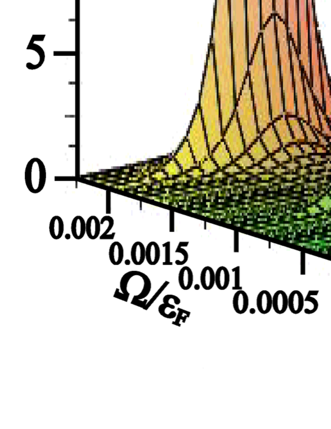
Figure 2: (Color online) (a) The angular frequency dependence of the SRT; $\bar{\mathcal{T}}_{{\rm{s}}}^{z}(0)$. A sharp peak exists on the point where the resonance condition, $\Omega=J$, is satisfied. Each quantity, $\bar{\mathcal{T}}_{{\rm{s}}}^{z}(\pm 1)$, has the same structure with $\bar{\mathcal{T}}_{{\rm{s}}}^{z}(0)$. (b) The time evolution of the SRT, ${\mathcal{T}}_{{\rm{s}}}^{z}/\Lambda$, at the resonance point ($\Omega=J$); (i) $0.446\times{\rm{cos}}^{2}(\Omega_{0}t)$, (ii) $0.112\times{\rm{cos}}^{2}(\Omega_{0}t/2)$, (iii) $0.0281\times{\rm{cos}}^{2}(\Omega_{0}t/4)$, where $\Omega_{0}\equiv 1.70\times 10^{13}$ $s^{-1}$.

4.3 Resonance

The SRT (eq. (32)), ${\mathcal{T}}_{{\rm{s}}}^{z}$, is rewritten as (see also Appendix B)

$${\mathcal{T}}_{\rm{s}}^{z} \equiv \Lambda\int_{0}^{\infty}(\sqrt{\frac{F}{\epsilon_{\rm{F}}}}dk)\ \bar{\mathcal{T}}_{{\rm{s}}}^{z},\ \rm{where}$$ (48)

$$\bar{\mathcal{T}}_{{\rm{s}}}^{z} = \sum_{n=0,\pm 1}\bar{\mathcal{T}}_{\rm{s}}^{z}(n)\ {\rm{e}}^{2in\Omega t},$$ (49)

$$\Lambda = \frac{\sqrt{\epsilon_{\rm{F}}}S{{{\Gamma}_{0}}}^{2}}{4(2\pi\sqrt{F})^{3}}.$$ (50)

The variable, $\bar{\mathcal{T}}_{{\rm{s}}}^{z}$, is the dimensionless SRT as a function of the wavenumber for conduction electrons $\sqrt{F/\epsilon_{\rm{F}}}k$, the angular frequency of the applied transverse magnetic field $\Omega/\epsilon_{\rm{F}}$, the magnitude of the exchange interaction $J/\epsilon_{\rm{F}}$, and so on. Fig. 2 (a) represents the

$$\bar{\mathcal{T}}_{\rm{s}}^{z}(0),$$ (51)

which is the time average of $\bar{\mathcal{T}}_{\rm{s}}^{z}$. Fig. 2 (b) shows

$${\mathcal{T}}_{\rm{s}}^{z}/\Lambda$$ (52)

(see eq. (48)), which describes the time evolution of the SRT. We have set each parameter, as a typical case,[14, 24, 3, 25] as follows; $\epsilon_{\rm{F}}=5.6$ eV, $B/{\epsilon_{\rm{F}}}=1.2\times 10^{-5}$, $T=300$ K, $F=4$ eV Ų, $D=0.3$ eV Ų, ${\tau}=1$ ps $={10^{-3}}\times{\tau}_{\rm{m}}$, $a_{0}=3$ Å, $S=1/2$.

Fig. 2 (a) shows that the SRT has a sharp peak as a result of the resonance with the angular frequency, $\Omega$, of the applied transverse magnetic field. The sharp peak exists on the point where the condition,

$$\Omega=J,$$ (53)

is satisfied. This is because according to eq. (7), the localized spin acts as an effective magnetic field along the quantization axis $J$, which is far larger than the applied magnetic field $B$;

$${\cal{H}}_{\rm{ex}}^{S=1/2}=-J{\int_{{\mathbf{x}}\in\text{(interface)}}}d{\mathbf{x}}{\ }s^{z}({\mathbf{x}},t).$$ (54)

This fact (i.e. resonance condition) is useful to enhance the spin pumping effect because the angular frequency of a transverse magnetic field is under our control. In addition Fig. 2 (a) also shows that the stronger the exchange interaction becomes, the larger the SRT does. Fig. 2 (b) shows ${\mathcal{T}}_{{\rm{s}}}^{z}/\Lambda$ at the resonance point ($\Omega=J$). Each period reads

$$\pi/\Omega.$$ (55)

5 Distinction from the Theory Proposed by Tserkovnyak et al.

Last, let us discuss the distinction between our quantum spin pumping theory[26] and the one proposed by Tserkovnyak et al.[2] It should be noted that, as has been mentioned in their article[2] (see §VIII. SUMMARY AND OUTLOOK in their article[2]), they have phenomenologically treated the spin-flip scattering processes, which we have regarded as the most important processes for spin pumping. Nevertheless, now their spin pumping theory has been widely used for interpreting vast experimental results,[14, 27, 30, 31] in particular by experimentalists. Thus, it would be significant to clarify the difference between our quantum spin pumping theory and the one proposed by Tserkovnyak et al.

5.1 The spin pumping theory proposed by Tserkovnyak et al.

According to the phenomenological[2, 30] spin pumping theory by Tserkovnyak et al. and their notation,[32, 2] the pumped spin current ${\mathbf{I}}_{\rm{s{\mathchar 45\relax}pump}}$ reads

$${\mathbf{I}}_{\rm{s{\mathchar 45\relax}pump}}={\rm{G}}_{\perp}^{(\rm{R})}{\mathbf{m}}\times\dot{\mathbf{m}}+{\rm{G}}_{\perp}^{(\rm{I})}\dot{\mathbf{m}},$$ (56)

where the dot denotes the time derivative. We have taken ${e}=1$, and ${\mathbf{m}}({\mathbf{x}},t)$ denotes a unit vector along the magnetization direction; they have treated ${\mathbf{m}}({\mathbf{x}},t)$ as classical variables. The variable ${\rm{G}}_{\perp}$ is the complex-valued mixing conductance that depends on the material;[33, 34] ${\rm{G}}_{\perp}={\rm{G}}_{\perp}^{(\rm{R})}+i{\rm{G}}_{\perp}^{(\rm{I})}$.

5.2 Landau-Lifshitz-Gilbert equation

The magnetization dynamics of ferromagnets can be described by the Landau-Lifshitz-Gilbert (LLG) eq.;

$$\dot{\mathbf{m}}=\gamma{\mathbf{H}}_{\rm{eff}}\times{\mathbf{m}}+\alpha{\mathbf{m}}\times\dot{\mathbf{m}},$$ (57)

where $\gamma$ is the gyro-magnetic ratio and $\alpha$ is the Gilbert damping constant that determines the magnetization dissipation rate. Here it should be emphasized that though this Gilbert damping constant, $\alpha$, was phenomenologically introduced,[35] it can be derived microscopically by considering a whole system including spin relaxation;[36] thus the effect of the exchange coupling to conduction electrons should be considered to have already been included into this Gilbert damping term.

The effective magnetic field is set as

$${\mathbf{H}}_{\rm{eff}}=(\Gamma(t),0,B),$$ (58)

where $\Gamma(t)$ represents a time-dependent transverse magnetic field. The LLG eq., eq. (57), becomes

$$\begin{pmatrix}\dot{\rm{m}}^{x}\\ \dot{\rm{m}}^{y}\\ \dot{\rm{m}}^{z}\end{pmatrix}=\gamma\begin{pmatrix}-B{\rm{m}^{y}}\\ B{\rm{m}^{x}}-\Gamma{\rm{m}^{z}}\\ \Gamma{\rm{m}^{y}}\end{pmatrix}+\alpha\begin{pmatrix}{\rm{m}^{y}}\dot{{\rm{m}}}^{z}-\dot{{\rm{m}}}^{y}{\rm{m}^{z}}\\ {\rm{m}^{z}}\dot{{\rm{m}}}^{x}-\dot{{\rm{m}}}^{z}{\rm{m}^{x}}\\ {\rm{m}^{x}}\dot{{\rm{m}}}^{y}-\dot{{\rm{m}}}^{x}{\rm{m}^{y}}\end{pmatrix}.$$ (59)

5.3 Pumped spin currents based on the theory by Tserkovnyak et al. at finite temperature

Eq. (59) is substituted into ${\rm{I}}_{\rm{s{\mathchar 45\relax}pump}}^{z}$, eq. (56); we include the contribution of the Gilbert damping term, which depends on the materials, up to ${\cal{O}}(\alpha)$; $\alpha\sim 10^{-3},10^{-2}$ for ${\rm{Ni}}_{81}{\rm{Fe}}_{19}$ (metal),[14] and $\alpha\sim 10^{-5}$ for ${\rm{Y}}_{3}{\rm{Fe}}_{5}{\rm{O}}_{12}$ (insulator),[3] as examples. Their theory is applicable to both ferromagnetic metals and insulators.[37]

Consequently, the z-component of the pumped spin current reads

$${\rm{I}}_{\rm{s{\mathchar 45\relax}pump}}^{z} = {\rm{G}}_{\perp}^{(\rm{R})}\Big{\{}\gamma B[({\rm{m}}^{x})^{2}+({\rm{m}}^{y})^{2}]-\gamma\Gamma{\rm{m}}^{x}{\rm{m}}^{z}-\alpha\gamma\Gamma[{\rm{m}}^{x}{\rm{m}}^{y}{\rm{m}}^{x}+({\rm{m}}^{y})^{3}+({\rm{m}}^{z})^{2}{\rm{m}}^{y}]\Big{\}}$$ (60)

$$+ {\rm{G}}_{\perp}^{(\rm{I})}\Big{\{}\alpha\gamma\{B[({\rm{m}}^{x})^{2}+({\rm{m}}^{y})^{2}]-\Gamma{\rm{m}}^{x}{\rm{m}}^{z}\}+\gamma\Gamma{\rm{m}}^{y}\Big{\}}+{\cal{O}}(\alpha^{2}).$$

$$\stackrel{{\scriptstyle\Gamma\rightarrow 0}}{{\longrightarrow}} [{\rm{G}}_{\perp}^{(\rm{R})}+\alpha{\rm{G}}_{\perp}^{(\rm{I})}]\gamma B[({\rm{m}}^{x})^{2}+({\rm{m}}^{y})^{2}].$$ (61)

$$\stackrel{{\scriptstyle{\rm{G}}_{\perp}^{(\rm{I})}\rightarrow 0}}{{\longrightarrow}} {\rm{G}}_{\perp}^{(\rm{R})}\gamma B[({\rm{m}}^{x})^{2}+({\rm{m}}^{y})^{2}].$$ (62)

At finite temperature, the magnetization is thermally activated; $\dot{\mathbf{m}}\not=0$.[24] Then the time derivative of the z-component means

$$\dot{\rm{m}}^{z} = \gamma\Gamma{\rm{m}}^{y}+\alpha\gamma\{B[({\rm{m}}^{x})^{2}+({\rm{m}}^{y})^{2}]-\Gamma{\rm{m}}^{x}{\rm{m}}^{z}\}+{\cal{O}}(\alpha^{2}).$$ (63)

$$\stackrel{{\scriptstyle\Gamma\rightarrow 0}}{{\longrightarrow}} \alpha\gamma B[({\rm{m}}^{x})^{2}+({\rm{m}}^{y})^{2}].$$ (64)

$$\not= 0.$$ (65)

5.4 Distinction

Eqs. (61), (62) and (65) mean that, within the framework by Tserkovnyak et al. with the LLG eq., they may gain spin currents at finite temperature if only the magnetic field along the z-axis, $B$, is applied;

$${\rm{I}}_{\rm{s{\mathchar 45\relax}pump}}^{z}\stackrel{{\scriptstyle\Gamma\rightarrow 0(B\not=0)}}{{\nrightarrow}}0.$$ (66)

That is, the spin pumping theory by Tserkovnyak et al.[2, 32, 37] with the LLG eq. concludes that spin currents may be pumped at finite temperature without time-dependent transverse magnetic fields.

On the other hand, as discussed in the last section (see eqs. (46) and (47)), our approach based on the Schwinger-Keldysh formalism gives different result;

$${\mathcal{T}}_{\rm{s}}^{z}\stackrel{{\scriptstyle\Gamma\rightarrow 0}}{{\longrightarrow}}0.$$ (67)

That is, our quantum spin pumping theory means that spin currents mediated by magnons cannot be pumped without quantum fluctuations (i.e. time-dependent transverse magnetic fields, $\Gamma(t)$); quantum fluctuations are essential to spin pumping mediated by magnons as well as the exchange interaction between conduction electrons and ferromagnets.

This (eqs. (67) and (66)) is the significant distinction between our quantum spin pumping theory and the one proposed by Tserkovnyak et al.

6 Summary and Discussion

We have microscopically studied quantum spin pumping mediated by magnons by evaluating the SRT at room temperature. Localized spins of the ferromagnetic insulator lose spin angular momentum by emitting a magnon and conduction electrons flip from down to up by absorbing the momentum. Thus our formalism contains no phenomenological treatments of spin-flip scattering processes. The SRT breaking the spin conservation law represents the (net) spin current mediated by magnons, which is pumped into the adjacent non-magnetic metal.

Through the Schwinger-Keldysh formalism, we have clarified that quantum fluctuations (i.e. time-dependent transverse magnetic fields) induce a net spin current, which can be enhanced through a resonance structure as a function of the angular frequency of the applied transverse field. We conclude that the breaking of the spin conservation law and quantum fluctuations are essential to quantum spin pumping mediated by magnons accompanying the exchange interaction.

In this paper, we have theoretically introduced and defined the interface as an effective area where the Fermi gas (conduction electrons) and the Bose gas (magnons) coexist to interact. Though the behavior of the quantum spin pumping effect mediated by magnons can be qualitatively captured by calculating the SRT, the theoretical estimation for the volume, in particular the width, of the interface is essential for the quantitative understanding. Of course the width of the interface may be roughly supposed to be of the order of the lattice constant, but we consider microscopic derivation (so called proximity effects) is an urgent theoretical issue.

In addition, though we have not executed vertex corrections at the present study in order to clarify that pumped spin currents are generated purely by quantum fluctuations, calculating the SRT under the effects of vertex corrections (i.e. multiple scatterings of impurities) as well as quantum fluctuations is a significant theoretical issue. Also from viewpoints of theoretical aspects (i.e. quantum field theory), it might be better to execute vertex corrections. Thus, we would like to tackle this issue in the near future.

In the present study, we have focused exclusively on the dynamics at the interface ($J\not=0$), where pumped spin currents are generated with interchanging spin angular momentum between conduction electrons and magnons. Then, our quantum spin pumping theory microscopically well describes the dynamics of generating pumped spin currents, in particular, the spin-flip scattering processes, which we have regarded as the most important processes for spin pumping. This is the strong point of our theory; note that the theory proposed by Tserkovnyak et al. has phenomenologically treated spin-flip processes.[2] On the other hand, the dynamics of pumped spin currents in the non-magnetic metal ($J=0$), i.e. how the pumped spin currents flow in the non-magnetic metal, is out of the application (purpose) of the present our theory. That is, though our formalism has microscopically captured the spin-flip scattering processes at the interface beyond phenomenology, it does not cover the dynamics of pumped spin currents; the dynamics under the existence of pumped spin currents such as the effect of localized spins and conduction electrons on pumped spin currents, which is often indicated as the $\beta$ term,[19, 28, 29] is out of the application (purpose) of the present study. Therefore, we would like to brush up our quantum spin pumping theory to cover the dynamics of pumped spin currents in the non-magnetic metal; how the pumped spin currents flow in the non-magnetic metal. We recognize that clarifying these issues is significant from viewpoints of applications as well as fundamental science.

Last, we have revealed that magnons accompanying the exchange interaction cannot contribute to quantum spin pumping without quantum fluctuations. Here it should be stressed that in our formalism, the meditation of spin angular momentum is restricted to only magnons. We will take the effect of phonons into account and develop our theory as a more rigorous formalism to reveal the microscopic (quantum) dynamics of the magnon splitting.[4, 27] Moreover, we are also interested in the contribution of magnons to quantum spin pumping under a spatially nonuniform magnetization.

Appendix A Langreth Method

In this section, we show how to calculate eqs. (28)-(31) in detail.

First, we briefly show the Langreth method,[12, 18, 19, 20] which is useful to evaluate the perturbation expansion of the Keldysh ( or contour-ordered) Green’s function[16, 17, 20, 19, 18] in subsection A.1. Second, we introduce the point of the bosonic Keldysh Green’s functions[16, 17, 20, 21] in subsection A.2. Last, the detailed calculations of eqs. (28)-(31) are represented in subsection A.3.

We omit the label, ${\mathbf{x}}$, when it is not relevant.

A.1 The Schwinger-Keldysh closed time path; a concrete example

For simplicity here, we consider the perturbative term, $V^{\prime}$,

$$V^{\prime}=\Gamma(t)\int d{\mathbf{x}}[a(\mathbf{x},t)+a^{\dagger}(\mathbf{x},t)],$$ (68)

and evaluate the expectation value of the bosonic annihilate operator, $a$, as an example;

$$\langle a(\tau)\rangle = \Big{\langle}\text{T}_{\text{c}}\ a(\tau)\text{exp}[-i\int_{\text{c}}d\tau^{\prime}V(\tau^{\prime})]\Big{\rangle}$$ (69)

$$= -i\int d{\mathbf{x}}^{\prime}\int_{\text{c}}d\tau^{\prime}\Gamma(\tau^{\prime})\langle\text{T}_{\text{c}}\ a(\mathbf{x},\tau)a^{\dagger}(\mathbf{x^{\prime}},\tau^{\prime})\rangle+{\cal{O}}(\Gamma^{2})$$ (70)

$$\equiv -i\int d{\mathbf{x}}^{\prime}{\cal{I}}.\;$$ (71)

Here $\text{T}_{\text{c}}$ is the path-ordering operator defined on the Schwinger-Keldysh closed time path,[21] c (see Fig. A$\cdot$1 in our manuscript[12, 17, 19, 18]) We express the Schwinger-Keldysh closed time path as a sum of the forward path, $c_{\rightarrow}$, and the backward path, $c_{\leftarrow}$; $c=c_{\rightarrow}+c_{\leftarrow}$.[21, 17, 19, 18] We take $\tau$ which denotes the contour variable defined on the Schwinger-Keldysh closed time path on forward path, ${\rm{c}}_{\rightarrow}$. Even when $\tau$ is located on backward path, ${\rm{c}}_{\leftarrow}$, the result of this calculation is invariant because each Green’s function, $\rm{G}^{\rm{r}}$, $\rm{G}^{\rm{a}}$, $\rm{G}^{\rm{<}}$, $\rm{G}^{\rm{>}}$, is not independent;[17, 16, 20, 19] they obey,

$$\rm{G}^{\rm{r}}-\rm{G}^{\rm{a}}=\rm{G}^{\rm{>}}-\rm{G}^{\rm{<}}.$$ (72)

Note that this relation comes into effect also for the fermionic case;[17, 16, 20, 19]

$${\mathcal{G}}^{\text{r}}-{\mathcal{G}}^{\text{a}}={\mathcal{G}}^{\text{>}}-{\mathcal{G}}^{\text{<}}.$$ (73)

The integral on the Schwinger-Keldysh closed time path of eq. (71), ${\cal{I}}$, is executed by taking an identity[17, 20] into account

$$\begin{split}\int_{{\text{c}}}d\tau^{\prime}&=\int_{{\text{c}}_{\rightarrow}}d\tau^{\prime}+\int_{{\text{c}}_{\leftarrow}}d\tau^{\prime},\\ \;\end{split}$$ (74)

as (see also eq. (78) in Appendix A.2)

$$\begin{split}{\cal{I}}=i\int_{-\infty}^{\infty}dt^{\prime}\Gamma(t^{\prime})[{\rm{G}}^{\rm{t}}(t,t^{\prime})-{\rm{G}}^{\rm{<}}(t,t^{\prime})].\;\end{split}$$ (75)

By using the relation, ${\rm{G}}^{\text{r}}(t,t^{\prime})={\rm{G}}^{\text{t}}(t,t^{\prime})-{\rm{G}}^{\text{<}}(t,t^{\prime})$, we obtain

$$\begin{split}{\cal{I}}=i\int_{-\infty}^{\infty}dt^{\prime}\Gamma(t^{\prime}){\rm{G}}^{\rm{r}}(t,t^{\prime}).\end{split}$$ (76)

A.2 Bosonic Keldysh Green’s function

In this subsection, we show the point of the bosonic Keldysh Green’s functions.

The bosonic Keldysh Green’s function, ${\rm{G}}(\tau,\tau^{\prime})$, is defined as[16, 17, 20]

$${\rm{G}}(\tau,\tau^{\prime}):=-i\langle\text{T}_{\text{c}}a(\tau)a^{\dagger}(\tau^{\prime})\rangle.$$ (77)

Depending on the points where $\tau$ and $\tau^{\prime}$ are located on the Schwinger-Keldysh closed time path (i.e. $\rm{c}={{\text{c}}_{\rightarrow}}+{{\text{c}}_{\leftarrow}}$), the bosonic Keldysh Green’s function is expressed as[16, 17, 20]

$${\rm{G}}(\tau,\tau^{\prime})=\begin{cases}{\rm{G}}^{\rm{<}}(t,t^{\prime})=-i\langle a^{\dagger}(t^{\prime})a(t)\rangle,&{\rm{when}}\ \tau\in{{\text{c}}_{\rightarrow}},\tau^{\prime}\in{{\text{c}}_{\leftarrow}}.\\ {\rm{G}}^{\rm{>}}(t,t^{\prime})=-i\langle a(t)a^{\dagger}(t^{\prime})\rangle,&{\rm{when}}\ \tau\in{{\text{c}}_{\leftarrow}},\tau^{\prime}\in{{\text{c}}_{\rightarrow}}.\\ {\rm{G}}^{\rm{t}}(t,t^{\prime}),&{\rm{when}}\ \tau\in{{\text{c}}_{\rightarrow}},\tau^{\prime}\in{{\text{c}}_{\rightarrow}}.\\ {\rm{G}}^{\bar{\rm{t}}}(t,t^{\prime}),&{\rm{when}}\ \tau\in{{\text{c}}_{\leftarrow}},\tau^{\prime}\in{{\text{c}}_{\leftarrow}}.\end{cases}$$ (78)

It should be noted that each Green’s function is not independent;[16, 17, 20]

$$\rm{G}^{\rm{r}}-\rm{G}^{\rm{a}}=\rm{G}^{\rm{>}}-\rm{G}^{\rm{<}}\Leftrightarrow\rm{G}^{\rm{t}}+\rm{G}^{\bar{\rm{t}}}=\rm{G}^{\rm{>}}+\rm{G}^{\rm{<}}.$$ (79)

In addition, these relations[20, 21] would be useful on calculation;

$$\rm{G}^{\rm{t}} = \rm{G}^{\rm{a}}+\rm{G}^{\rm{>}},$$ (80)

$$\rm{G}^{\bar{\rm{t}}} = \rm{G}^{\rm{<}}-\rm{G}^{\rm{a}},$$ (81)

$$\rm{G}^{\rm{r}} = \rm{G}^{\rm{t}}-\rm{G}^{\rm{<}}$$ (82)

$$= \rm{G}^{\rm{>}}-\rm{G}^{\bar{\rm{t}}},$$ (83)

$$\langle a^{\dagger}(t)a(t)\rangle = i{\rm{G}}^{\rm{<}}(t,t).$$ (84)

By executing the Fourier transformation, the lesser and greater Green’s functions for free bosons become[16, 20]

$${\rm{G}}^{\rm{<}}_{{\mathbf{k^{\prime}}},\omega^{\prime}} = -f_{\rm{B}}(\omega^{\prime})({\rm{G}}^{\rm{a}}_{{\mathbf{k^{\prime}}},\omega^{\prime}}-{\rm{G}}^{\rm{r}}_{{\mathbf{k^{\prime}}},\omega^{\prime}})$$ (85)

$$= -2\pi if_{\rm{B}}(\omega^{\prime})\delta(\omega^{\prime}-\omega_{{\mathbf{k^{\prime}}}}),$$ (86)

$${\rm{G}}^{\rm{>}}_{{\mathbf{k^{\prime}}},\omega^{\prime}} = -2\pi i[1+f_{\rm{B}}(\omega^{\prime})]\delta(\omega^{\prime}-\omega_{{\mathbf{k^{\prime}}}}),$$ (87)

$${\rm{G}}^{\rm{K}}_{{\mathbf{k^{\prime}}},\omega^{\prime}} := {\rm{G}}^{\rm{<}}_{{\mathbf{k^{\prime}}},\omega^{\prime}}+{\rm{G}}^{\rm{>}}_{{\mathbf{k^{\prime}}},\omega^{\prime}}$$ (88)

$$= -2\pi i[1+2f_{\rm{B}}(\omega^{\prime})]\delta(\omega^{\prime}-\omega_{{\mathbf{k^{\prime}}}})$$ (89)

$$= 2i{\rm{Im}}{\rm{G}}^{\rm{r}}_{{\mathbf{k^{\prime}}},\omega^{\prime}}{\rm{coth}}(\beta\omega^{\prime}/2).$$ (90)

The last one, ${\rm{G}}^{\rm{K}}$, represents the Keldysh Green’s function [16, 17] and the relation is called the bosonic fluctuation-dissipation theorem.[21]

Fermionic Keldysh Green’s function

It would be useful to compare with the (spinless) Fermionic Keldysh Green’s function, ${\mathcal{G}}(\tau,\tau^{\prime})$, which is defined as[16, 17, 20, 19, 18]

$${\mathcal{G}}(\tau,\tau^{\prime}):=-i\langle\text{T}_{\text{c}}c(\tau)c^{\dagger}(\tau^{\prime})\rangle.$$ (91)

Depending on the points where $\tau$ and $\tau^{\prime}$ are located on the Schwinger-Keldysh closed time path (i.e. $\rm{c}={{\text{c}}_{\rightarrow}}+{{\text{c}}_{\leftarrow}}$), the Fermionic Keldysh Green’s function is expressed as[16, 17, 20, 19, 18]

$${\mathcal{G}}(\tau,\tau^{\prime})=\begin{cases}{\mathcal{G}}^{\rm{<}}(t,t^{\prime})=i\langle c^{\dagger}(t^{\prime})c(t)\rangle,&{\rm{when}}\ \tau\in{{\text{c}}_{\rightarrow}},\tau^{\prime}\in{{\text{c}}_{\leftarrow}}.\\ {\mathcal{G}}^{\rm{>}}(t,t^{\prime})=-i\langle c(t)c^{\dagger}(t^{\prime})\rangle,&{\rm{when}}\ \tau\in{{\text{c}}_{\leftarrow}},\tau^{\prime}\in{{\text{c}}_{\rightarrow}}.\\ {\mathcal{G}}^{\rm{t}}(t,t^{\prime}),&{\rm{when}}\ \tau\in{{\text{c}}_{\rightarrow}},\tau^{\prime}\in{{\text{c}}_{\rightarrow}}.\\ {\mathcal{G}}^{\bar{\rm{t}}}(t,t^{\prime}),&{\rm{when}}\ \tau\in{{\text{c}}_{\leftarrow}},\tau^{\prime}\in{{\text{c}}_{\leftarrow}}.\end{cases}$$ (92)

Note that with reflecting the statistical properties, the sign of the lesser Green’s function is opposite from the bosonic case. In addition, they satisfy the relation;[16, 17, 20, 19, 18]

$$\mathcal{G}^{\rm{r}}-\mathcal{G}^{\rm{a}}=\mathcal{G}^{\rm{>}}-\mathcal{G}^{\rm{<}}\Leftrightarrow\mathcal{G}^{\rm{t}}+\mathcal{G}^{\bar{\rm{t}}}=\mathcal{G}^{\rm{>}}+\mathcal{G}^{\rm{<}},$$ (93)

$$\mathcal{G}^{\rm{t}} = \mathcal{G}^{\rm{r}}+\mathcal{G}^{\rm{<}}$$ (94)

$$= \mathcal{G}^{\rm{a}}+\mathcal{G}^{\rm{>}},$$ (95)

$$\mathcal{G}^{\bar{\rm{t}}} = -\mathcal{G}^{\rm{r}}+\mathcal{G}^{\rm{>}}$$ (96)

$$= -\mathcal{G}^{\rm{a}}+\mathcal{G}^{\rm{<}}.$$ (97)

By executing the Fourier transformation, the lesser and greater Green’s functions for free Fermions become[16, 20, 19, 18]

$${\mathcal{G}}^{\rm{<}}_{{\mathbf{k}},\omega} = f_{\rm{F}}(\omega)({\mathcal{G}}^{\rm{a}}_{{\mathbf{k}},\omega}-{\mathcal{G}}^{\rm{r}}_{{\mathbf{k}},\omega})$$ (98)

$$= 2\pi if_{\rm{F}}(\omega)\delta(\omega-\omega_{{\mathbf{k}}}),$$ (99)

$${\mathcal{G}}^{\rm{>}}_{{\mathbf{k}},\omega} = -2\pi i[1-f_{\rm{F}}(\omega)]\delta(\omega-\omega_{{\mathbf{k}}}),$$ (100)

$${\mathcal{G}}^{\rm{K}}_{{\mathbf{k}},\omega} := {\mathcal{G}}^{\rm{<}}_{{\mathbf{k}},\omega}+{\mathcal{G}}^{\rm{>}}_{{\mathbf{k}},\omega}$$ (101)

$$= -2\pi i[1-2f_{\rm{F}}(\omega)]\delta(\omega-\omega_{{\mathbf{k}}})$$ (102)

$$= 2i{\rm{Im}}{\mathcal{G}}^{\rm{r}}_{{\mathbf{k}},\omega}{\rm{tanh}}(\beta\omega/2).$$ (103)

The last one, ${\mathcal{G}}^{\rm{K}}$, represents the Keldysh Green’s function [16, 17] and the relation is called the fermionic fluctuation-dissipation theorem.[21, 18]

A.3 Detail of the calculation; eqs. (28)-(31)

In this subsection, we will briefly show how to calculate eqs. (28)-(31).

By adopting the Wick’s theorem,[17, 21] the left-hand side (LHS) of eq. (28) reads

$$\begin{split}({\rm{The\ LHS\ of\ }}{\rm{eq}}.(\ref{eqn:e6}))&=\frac{iJa_{0}^{3}{\tilde{S}}}{2}\int d{\mathbf{x}}^{\prime}\int d{\mathbf{x}}^{\prime\prime}\int_{{\text{c}}}d\tau^{\prime}\int_{{\text{c}}}d\tau^{\prime\prime}\Gamma(\tau^{\prime})\Gamma(\tau^{\prime\prime})\Big{(}1-\frac{\langle\text{T}_{\text{c}}\ a^{\dagger}({\mathbf{x}}^{\prime},\tau^{\prime})a({\mathbf{x}}^{\prime},\tau^{\prime})\rangle}{\tilde{S}}\Big{)}\\ &\times\langle\text{T}_{\text{c}}\ a({\mathbf{x}}^{\prime\prime},\tau^{\prime\prime})a^{\dagger}({\mathbf{x}},\tau)\rangle\langle\text{T}_{\text{c}}\ c_{\downarrow}({\mathbf{x}},\tau)c_{\downarrow}^{\dagger}({\mathbf{x}^{\prime}},\tau^{\prime})\rangle\langle\text{T}_{\text{c}}\ c_{\uparrow}({\mathbf{x}}^{\prime},\tau^{\prime})c_{\uparrow}^{\dagger}({\mathbf{x}},\tau)\rangle.\end{split}$$ (104)

By employing the relation;

$$\int_{{\text{c}}}d\tau^{\prime}\int_{{\text{c}}}d\tau^{\prime\prime} = \Big{(}\int_{{\text{c}}_{\rightarrow}}d\tau^{\prime}+\int_{{\text{c}}_{\leftarrow}}d\tau^{\prime}\Big{)}\Big{(}\int_{{\text{c}}_{\rightarrow}}d\tau^{\prime\prime}+\int_{{\text{c}}_{\leftarrow}}d\tau^{\prime\prime}\Big{)}$$

$$= \int_{{\text{c}}_{\rightarrow}}d\tau^{\prime}\int_{{\text{c}}_{\rightarrow}}d\tau^{\prime\prime}+\int_{{\text{c}}_{\rightarrow}}d\tau^{\prime}\int_{{\text{c}}_{\leftarrow}}d\tau^{\prime\prime}$$

$$+ \int_{{\text{c}}_{\leftarrow}}d\tau^{\prime}\int_{{\text{c}}_{\rightarrow}}d\tau^{\prime\prime}+\int_{{\text{c}}_{\leftarrow}}d\tau^{\prime}\int_{{\text{c}}_{\leftarrow}}d\tau^{\prime\prime},$$ (106)

and the Langreth method[18, 19, 20] with eqs. (78) and (92), the right-hand side (RHS) of eq. (104) can be expressed as

$$\begin{split}(\rm{The\ RHS\ of\ }{\rm{eq}}.(\ref{eqn:a10}))&=\frac{Ja_{0}^{3}\tilde{S}}{2}\int d{\mathbf{x}}^{\prime}\int d{\mathbf{x}}^{\prime\prime}\int_{-\infty}^{\infty}dt^{\prime}\int_{-\infty}^{\infty}dt^{\prime\prime}\Gamma(t^{\prime})\Gamma(t^{\prime\prime})\Big{(}1-\frac{i}{\tilde{S}}{\rm{G}}^{\rm{<}}(t^{\prime},t^{\prime})\Big{)}\\ &\times[{\rm{G}}^{\rm{t}}(t^{\prime\prime},t)-{\rm{G}}^{\rm{>}}(t^{\prime\prime},t)][{\cal{G}}_{\downarrow}^{\rm{t}}(t,t^{\prime}){\cal{G}}_{\uparrow}^{\rm{t}}(t^{\prime},t)-{\cal{G}}_{\downarrow}^{\rm{<}}(t,t^{\prime}){\cal{G}}_{\uparrow}^{\rm{>}}(t^{\prime},t)].\end{split}$$ (107)

We also here have taken $\tau$ on forward path, ${\rm{c}}_{\rightarrow}$. As discussed in the last subsection, even when $\tau$ is located on backward path, ${\rm{c}}_{\leftarrow}$, the result of this calculation is invariant.

Here it should be noted that

$${\rm{G}}^{\rm{t}}(t^{\prime\prime},t)-{\rm{G}}^{\rm{>}}(t^{\prime\prime},t)={\rm{G}}^{\rm{a}}(t^{\prime\prime},t).$$ (108)

Then, eq. (107) can be rewritten as

$$\begin{split}(\rm{The\ RHS\ of\ }{\rm{eq}}.(\ref{eqn:a11}))&=\frac{Ja_{0}^{3}\tilde{S}}{2}\int d{\mathbf{x}}^{\prime}\int d{\mathbf{x}}^{\prime\prime}\int_{-\infty}^{\infty}dt^{\prime}\int_{-\infty}^{\infty}dt^{\prime\prime}\Gamma(t^{\prime})\Gamma(t^{\prime\prime})\Big{(}1-\frac{i}{\tilde{S}}{\rm{G}}^{\rm{<}}(t^{\prime},t^{\prime})\Big{)}\\ &\times{\rm{G}}^{\rm{a}}(t^{\prime\prime},t)[{\cal{G}}_{\downarrow}^{\rm{t}}(t,t^{\prime}){\cal{G}}_{\uparrow}^{\rm{t}}(t^{\prime},t)-{\cal{G}}_{\downarrow}^{\rm{<}}(t,t^{\prime}){\cal{G}}_{\uparrow}^{\rm{>}}(t^{\prime},t)].\end{split}$$ (109)

By executing Fourier transformation, we obtain the RHS of eq. (28).

Through the same procedure, remained terms are evaluated as follows;

$$\begin{split}({\rm{The\ LHS\ of\ }}{\rm{eq}}.(\ref{eqn:e7}))&=-\frac{iJa_{0}^{3}{\tilde{S}}}{2}\int d{\mathbf{x}}^{\prime}\int d{\mathbf{x}}^{\prime\prime}\int_{{\text{c}}}d\tau^{\prime}\int_{{\text{c}}}d\tau^{\prime\prime}\Gamma(\tau^{\prime})\Gamma(\tau^{\prime\prime})\Big{(}1-\frac{\langle\text{T}_{\text{c}}\ a^{\dagger}({\mathbf{x}}^{\prime},\tau^{\prime})a({\mathbf{x}}^{\prime},\tau^{\prime})\rangle}{\tilde{S}}\Big{)}\\ &\times\langle\text{T}_{\text{c}}\ a({\mathbf{x}},\tau)a^{\dagger}({\mathbf{x}}^{\prime\prime},\tau^{\prime\prime})\rangle\langle\text{T}_{\text{c}}\ c_{\uparrow}({\mathbf{x}},\tau)c_{\uparrow}^{\dagger}({\mathbf{x}^{\prime}},\tau^{\prime})\rangle\langle\text{T}_{\text{c}}\ c_{\downarrow}({\mathbf{x}}^{\prime},\tau^{\prime})c_{\downarrow}^{\dagger}({\mathbf{x}},\tau)\rangle\\ &=-\frac{Ja_{0}^{3}\tilde{S}}{2}\int d{\mathbf{x}}^{\prime}\int d{\mathbf{x}}^{\prime\prime}\int_{-\infty}^{\infty}dt^{\prime}\int_{-\infty}^{\infty}dt^{\prime\prime}\Gamma(t^{\prime})\Gamma(t^{\prime\prime})\Big{(}1-\frac{i}{\tilde{S}}{\rm{G}}^{\rm{<}}(t^{\prime},t^{\prime})\Big{)}\\ &\times{\rm{G}}^{\rm{r}}(t,t^{\prime\prime})[{\cal{G}}_{\uparrow}^{\rm{t}}(t,t^{\prime}){\cal{G}}_{\downarrow}^{\rm{t}}(t^{\prime},t)-{\cal{G}}_{\uparrow}^{\rm{<}}(t,t^{\prime}){\cal{G}}_{\downarrow}^{\rm{>}}(t^{\prime},t)].\end{split}$$ (110)

$$\begin{split}({\rm{The\ LHS\ of\ }}{\rm{eq}}.(\ref{eqn:e8}))&=\frac{iJa_{0}^{3}{\tilde{S}}}{2}\int d{\mathbf{x}}^{\prime}\int d{\mathbf{x}}^{\prime\prime}\int_{{\text{c}}}d\tau^{\prime}\int_{{\text{c}}}d\tau^{\prime\prime}\Gamma(\tau)\Gamma(\tau^{\prime\prime})\Big{(}1-\frac{\langle\text{T}_{\text{c}}\ a^{\dagger}({\mathbf{x}}^{\prime},\tau^{\prime})a({\mathbf{x}}^{\prime},\tau^{\prime})\rangle}{\tilde{S}}\Big{)}\\ &\times\langle\text{T}_{\text{c}}\ a({\mathbf{x}}^{\prime},\tau^{\prime})a^{\dagger}({\mathbf{x}}^{\prime\prime},\tau^{\prime\prime})\rangle\langle\text{T}_{\text{c}}\ c_{\downarrow}({\mathbf{x}},\tau)c_{\downarrow}^{\dagger}({\mathbf{x}^{\prime}},\tau^{\prime})\rangle\langle\text{T}_{\text{c}}\ c_{\uparrow}({\mathbf{x}}^{\prime},\tau^{\prime})c_{\uparrow}^{\dagger}({\mathbf{x}},\tau)\rangle\\ &=\frac{Ja_{0}^{3}\tilde{S}}{2}\int d{\mathbf{x}}^{\prime}\int d{\mathbf{x}}^{\prime\prime}\int_{-\infty}^{\infty}dt^{\prime}\int_{-\infty}^{\infty}dt^{\prime\prime}\Gamma(t)\Gamma(t^{\prime\prime})\Big{(}1-\frac{i}{\tilde{S}}{\rm{G}}^{\rm{<}}(t^{\prime},t^{\prime})\Big{)}\\ &\times{\rm{G}}^{\rm{r}}(t^{\prime},t^{\prime\prime})[{\cal{G}}_{\downarrow}^{\rm{t}}(t,t^{\prime}){\cal{G}}_{\uparrow}^{\rm{t}}(t^{\prime},t)-{\cal{G}}_{\downarrow}^{\rm{<}}(t,t^{\prime}){\cal{G}}_{\uparrow}^{\rm{>}}(t^{\prime},t)].\end{split}$$ (111)

Note that we have adopted the relation; ${\rm{G}}^{\rm{t}}-{\rm{G}}^{\rm{<}}={\rm{G}}^{\rm{r}}={\rm{G}}^{\rm{>}}-{\rm{G}}^{\bar{\rm{t}}}$.

$$\begin{split}({\rm{The\ LHS\ of\ }}{\rm{eq}}.(\ref{eqn:e9}))&=-\frac{iJa_{0}^{3}{\tilde{S}}}{2}\int d{\mathbf{x}}^{\prime}\int d{\mathbf{x}}^{\prime\prime}\int_{{\text{c}}}d\tau^{\prime}\int_{{\text{c}}}d\tau^{\prime\prime}\Gamma(\tau)\Gamma(\tau^{\prime\prime})\Big{(}1-\frac{\langle\text{T}_{\text{c}}\ a^{\dagger}({\mathbf{x}}^{\prime},\tau^{\prime})a({\mathbf{x}}^{\prime},\tau^{\prime})\rangle}{\tilde{S}}\Big{)}\\ &\times\langle\text{T}_{\text{c}}\ a({\mathbf{x}}^{\prime\prime},\tau^{\prime\prime})a^{\dagger}({\mathbf{x}}^{\prime},\tau^{\prime})\rangle\langle\text{T}_{\text{c}}\ c_{\uparrow}({\mathbf{x}},\tau)c_{\uparrow}^{\dagger}({\mathbf{x}^{\prime}},\tau^{\prime})\rangle\langle\text{T}_{\text{c}}\ c_{\downarrow}({\mathbf{x}}^{\prime},\tau^{\prime})c_{\downarrow}^{\dagger}({\mathbf{x}},\tau)\rangle\\ &=-\frac{Ja_{0}^{3}\tilde{S}}{2}\int d{\mathbf{x}}^{\prime}\int d{\mathbf{x}}^{\prime\prime}\int_{-\infty}^{\infty}dt^{\prime}\int_{-\infty}^{\infty}dt^{\prime\prime}\Gamma(t)\Gamma(t^{\prime\prime})\Big{(}1-\frac{i}{\tilde{S}}{\rm{G}}^{\rm{<}}(t^{\prime},t^{\prime})\Big{)}\\ &\times{\rm{G}}^{\rm{a}}(t^{\prime\prime},t^{\prime})[{\cal{G}}_{\uparrow}^{\rm{t}}(t,t^{\prime}){\cal{G}}_{\downarrow}^{\rm{t}}(t^{\prime},t)-{\cal{G}}_{\uparrow}^{\rm{<}}(t,t^{\prime}){\cal{G}}_{\downarrow}^{\rm{>}}(t^{\prime},t)].\end{split}$$ (112)

Note that we have employed the relation; ${\rm{G}}^{\rm{<}}-{\rm{G}}^{\bar{\rm{t}}}={\rm{G}}^{\rm{a}}={\rm{G}}^{\rm{t}}-{\rm{G}}^{{\rm{>}}}$.

By using Fourier transformation, we obtain the RHS of eqs. (29)-(31).

Appendix B The Form of the Spin Relaxation Torque

Finally, let us write down the explicit form of the SRT. We have taken $\hbar=1$ and have introduced the dimensionless variables as follows; $\bar{\cal{O}}\equiv{\cal{O}}/{\epsilon_{\rm{F}}}$, except $\bar{T}\equiv k_{\rm{B}}T/{\epsilon_{\rm{F}}}$ and $\bar{\tau}\equiv{\epsilon_{\rm{F}}}\tau/(\hbar)$. The dimensionless wavenumber for conduction electrons has been rewritten; $\sqrt{F/\epsilon_{\rm{F}}}k\equiv y$.

The SRT (i.e. eq. (48)), ${\mathcal{T}}_{\rm{s}}^{z}$, reads

$${\cal{T}}_{\rm{s}}^{z}=({\rm{I}})+({\rm{II}}),$$ (113)

where

$$({\rm{I}}) := \bigg{\langle}iJa_{0}^{3}\sqrt{\frac{\tilde{S}}{2}}a^{\dagger}({\mathbf{x}},t)\Big{[}1-\frac{a^{\dagger}({\mathbf{x}},t)a({\mathbf{x}},t)}{4\tilde{S}}\Big{]}c^{\dagger}({\mathbf{x}},t)\sigma^{+}c({\mathbf{x}},t)\bigg{\rangle}+\bigg{\langle}\frac{\Gamma(t)c^{\dagger}({\mathbf{x}},t)\sigma^{+}c({\mathbf{x}},t)}{4i}\bigg{\rangle}$$

$$= \frac{JS}{4\pi}(\frac{\Gamma_{0}}{2})^{2}\int\frac{d{{\mathbf{k}}}}{(2\pi)^{3}}\int d\omega\Big{[}1-\frac{i}{\tilde{S}}\int\frac{d{{\mathbf{k}}}^{\prime}}{(2\pi)^{3}}\int\frac{d{\omega}^{\prime}}{2\pi}{\rm{G}}^{\rm{<}}_{{{\mathbf{k}}}^{\prime},\omega^{\prime}}\Big{]}$$

$$\times \Bigg{\{}\Big{[}{\rm{e}}^{2i\Omega t}{\rm{G}}^{\rm{a}}_{0,\Omega}+{\rm{G}}^{\rm{a}}_{0,-\Omega}+({\rm{e}}^{2i\Omega t}+1){\rm{G}}^{\rm{r}}_{0,-\Omega}\Big{]}\cdot\Big{[}{\mathcal{G}}^{\rm{t}}_{\downarrow,{\mathbf{k}},\omega-\Omega}{\mathcal{G}}^{\rm{t}}_{\uparrow,{\mathbf{k}},\omega}-{\mathcal{G}}^{\rm{<}}_{\downarrow,{\mathbf{k}},\omega-\Omega}{\mathcal{G}}^{\rm{>}}_{\uparrow,{\mathbf{k}},\omega}\Big{]}$$

$$+ \Big{[}{\rm{e}}^{-2i\Omega t}{\rm{G}}^{\rm{a}}_{0,-\Omega}+{\rm{G}}^{\rm{a}}_{0,\Omega}+({\rm{e}}^{-2i\Omega t}+1){\rm{G}}^{\rm{r}}_{0,\Omega}\Big{]}\cdot\Big{[}{\mathcal{G}}^{\rm{t}}_{\downarrow,{\mathbf{k}},\omega+\Omega}{\mathcal{G}}^{\rm{t}}_{\uparrow,{\mathbf{k}},\omega}-{\mathcal{G}}^{\rm{<}}_{\downarrow,{\mathbf{k}},\omega+\Omega}{\mathcal{G}}^{\rm{>}}_{\uparrow,{\mathbf{k}},\omega}\Big{]}\Bigg{\}}$$

$$+ {\cal{O}}(J^{2})+{\cal{O}}({(\Gamma_{0})}^{0})$$

$$= {\bar{J}}\int d\bar{\omega}\int_{0}^{\infty}dyy^{2}\Bigg{[}\frac{{\rm{e}}^{2i\Omega t}(\bar{\omega}-\bar{B}+\frac{i}{2\bar{\tau}_{\rm{m}}})}{(\bar{\Omega}-\bar{B})^{2}+(\frac{1}{2\bar{\tau}_{\rm{m}}})^{2}}-\frac{({\rm{e}}^{2i\Omega t}+2)(\bar{\Omega}+\bar{B})+{\rm{e}}^{2i\Omega t}\frac{i}{2\bar{\tau}_{\rm{m}}})}{(\bar{\Omega}+\bar{B})^{2}+(\frac{1}{2\bar{\tau}_{\rm{m}}})^{2}}\Bigg{]}$$

$$\times \Big{[}1-\frac{i}{\tilde{S}}\int\frac{d{{\mathbf{k}}}^{\prime}}{(2\pi)^{3}}\int\frac{d{\omega}^{\prime}}{2\pi}f_{\rm{B}}(\omega^{\prime})\frac{-i/{\tau_{\rm{m}}}}{(\omega^{\prime}-\omega_{{\mathbf{k^{\prime}}}})^{2}+[1/(2\tau_{\rm{m}})]^{2}}\Big{]}$$

$$\times \Bigg{\{}\frac{1}{\Big{[}\bar{\omega}-\bar{\Omega}-y^{2}-(\bar{J}S+\frac{\bar{B}}{2}+\bar{\mu})\Big{]}^{2}+(\frac{1}{2\bar{\tau}})^{2}}$$

$$\times \Bigg{[}\frac{i}{\bar{\tau}}\frac{1}{{\rm{e}}^{[{{y}}^{2}+(\bar{J}S+\bar{B}/2)-\bar{\mu}]/{\bar{T}}}+1}+\bar{\omega}-\bar{\Omega}-y^{2}-(\bar{J}S+\frac{\bar{B}}{2}+\bar{\mu})-\frac{i}{2\bar{\tau}}\Bigg{]}$$

$$\times \frac{1}{\Big{[}\bar{\omega}-y^{2}+(\bar{J}S+\frac{\bar{B}}{2}+\bar{\mu})\Big{]}^{2}+(\frac{1}{2\bar{\tau}})^{2}}\Bigg{[}\frac{i}{\bar{\tau}}\frac{1}{{\rm{e}}^{[{{y}}^{2}-(\bar{J}S+\bar{B}/2)-\bar{\mu}]/{\bar{T}}}+1}+\bar{\omega}-y^{2}+(\bar{J}S+\frac{\bar{B}}{2}+\bar{\mu})-\frac{i}{2\bar{\tau}}\Bigg{]}$$

$$- \frac{1}{{\bar{\tau}}^{2}}\frac{1}{\Big{[}\bar{\omega}-\bar{\Omega}-y^{2}-(\bar{J}S+\frac{\bar{B}}{2}+\bar{\mu})\Big{]}^{2}+(\frac{1}{2\bar{\tau}})^{2}}\cdot\frac{1}{{\rm{e}}^{[{{y}}^{2}+(\bar{J}S+\bar{B}/2)-\bar{\mu}]/{\bar{T}}}+1}$$

$$\times \frac{1}{\Big{[}\bar{\omega}-y^{2}+(\bar{J}S+\frac{\bar{B}}{2}+\bar{\mu})\Big{]}^{2}+(\frac{1}{2\bar{\tau}})^{2}}\cdot\Big{(}1-\frac{1}{{\rm{e}}^{[{{y}}^{2}-(\bar{J}S+\bar{B}/2)-\bar{\mu}]/{\bar{T}}}+1}\Big{)}\Bigg{\}}$$

$$+ {\bar{J}}\int d\bar{\omega}\int_{0}^{\infty}dyy^{2}\Bigg{[}\frac{{\rm{e}}^{-2i\Omega t}(\bar{\omega}-\bar{B}+\frac{i}{2\bar{\tau}_{\rm{m}}})}{(-\bar{\Omega}-\bar{B})^{2}+(\frac{1}{2\bar{\tau}_{\rm{m}}})^{2}}-\frac{({\rm{e}}^{-2i\Omega t}+2)(-\bar{\Omega}+\bar{B})+{\rm{e}}^{-2i\Omega t}\frac{i}{2\bar{\tau}_{\rm{m}}})}{(-\bar{\Omega}+\bar{B})^{2}+(\frac{1}{2\bar{\tau}_{\rm{m}}})^{2}}\Bigg{]}$$

$$\times \Big{[}1-\frac{i}{\tilde{S}}\int\frac{d{{\mathbf{k}}}^{\prime}}{(2\pi)^{3}}\int\frac{d{\omega}^{\prime}}{2\pi}f_{\rm{B}}(\omega^{\prime})\frac{-i/{\tau_{\rm{m}}}}{(\omega^{\prime}-\omega_{{\mathbf{k^{\prime}}}})^{2}+[1/(2\tau_{\rm{m}})]^{2}}\Big{]}$$

$$\times \Bigg{\{}\frac{1}{\Big{[}\bar{\omega}+\bar{\Omega}-y^{2}-(\bar{J}S+\frac{\bar{B}}{2}+\bar{\mu})\Big{]}^{2}+(\frac{1}{2\bar{\tau}})^{2}}$$

$$\times \Bigg{[}\frac{i}{\bar{\tau}}\frac{1}{{\rm{e}}^{[{{y}}^{2}+(\bar{J}S+\bar{B}/2)-\bar{\mu}]/{\bar{T}}}+1}+\bar{\omega}+\bar{\Omega}-y^{2}-(\bar{J}S+\frac{\bar{B}}{2}+\bar{\mu})-\frac{i}{2\bar{\tau}}\Bigg{]}$$

$$\times \frac{1}{\Big{[}\bar{\omega}-y^{2}+(\bar{J}S+\frac{\bar{B}}{2}+\bar{\mu})\Big{]}^{2}+(\frac{1}{2\bar{\tau}})^{2}}\Bigg{[}\frac{i}{\bar{\tau}}\frac{1}{{\rm{e}}^{[{{y}}^{2}-(\bar{J}S+\bar{B}/2)-\bar{\mu}]/{\bar{T}}}+1}+\bar{\omega}-y^{2}+(\bar{J}S+\frac{\bar{B}}{2}+\bar{\mu})-\frac{i}{2\bar{\tau}}\Bigg{]}$$

$$- \frac{1}{{\bar{\tau}}^{2}}\frac{1}{\Big{[}\bar{\omega}+\bar{\Omega}-y^{2}-(\bar{J}S+\frac{\bar{B}}{2}+\bar{\mu})\Big{]}^{2}+(\frac{1}{2\bar{\tau}})^{2}}\cdot\frac{1}{{\rm{e}}^{[{{y}}^{2}+(\bar{J}S+\bar{B}/2)-\bar{\mu}]/{\bar{T}}}+1}$$

$$\times \frac{1}{\Big{[}\bar{\omega}-y^{2}+(\bar{J}S+\frac{\bar{B}}{2}+\bar{\mu})\Big{]}^{2}+(\frac{1}{2\bar{\tau}})^{2}}\cdot\Big{(}1-\frac{1}{{\rm{e}}^{[{{y}}^{2}-(\bar{J}S+\bar{B}/2)-\bar{\mu}]/{\bar{T}}}+1}\Big{)}\Bigg{\}},$$

and

$$({\rm{II}}) := \bigg{\langle}-iJa_{0}^{3}\sqrt{\frac{\tilde{S}}{2}}\Big{[}1-\frac{a^{\dagger}({\mathbf{x}},t)a({\mathbf{x}},t)}{4\tilde{S}}\Big{]}a({\mathbf{x}},t)c^{\dagger}({\mathbf{x}},t)\sigma^{-}c({\mathbf{x}},t)\bigg{\rangle}+\bigg{\langle}-\frac{\Gamma(t)c^{\dagger}({\mathbf{x}},t)\sigma^{-}c({\mathbf{x}},t)}{4i}\bigg{\rangle}$$

$$= -\frac{JS}{4\pi}(\frac{\Gamma_{0}}{2})^{2}\int\frac{d{{\mathbf{k}}}}{(2\pi)^{3}}\int d\omega\Big{[}1-\frac{i}{\tilde{S}}\int\frac{d{{\mathbf{k}}}^{\prime}}{(2\pi)^{3}}\int\frac{d{\omega}^{\prime}}{2\pi}{\rm{G}}^{\rm{<}}_{{{\mathbf{k}}}^{\prime},\omega^{\prime}}\Big{]}$$

$$\times \Bigg{\{}\Big{[}{\rm{e}}^{2i\Omega t}{\rm{G}}^{\rm{r}}_{0,\Omega}+{\rm{G}}^{\rm{r}}_{0,-\Omega}+({\rm{e}}^{2i\Omega t}+1){\rm{G}}^{\rm{a}}_{0,-\Omega}\Big{]}\cdot\Big{[}{\mathcal{G}}^{\rm{t}}_{\uparrow,{\mathbf{k}},\omega-\Omega}{\mathcal{G}}^{\rm{t}}_{\downarrow,{\mathbf{k}},\omega}-{\mathcal{G}}^{\rm{<}}_{\uparrow,{\mathbf{k}},\omega-\Omega}{\mathcal{G}}^{\rm{>}}_{\downarrow,{\mathbf{k}},\omega}\Big{]}$$

$$+ \Big{[}{\rm{e}}^{-2i\Omega t}{\rm{G}}^{\rm{r}}_{0,-\Omega}+{\rm{G}}^{\rm{r}}_{0,\Omega}+({\rm{e}}^{-2i\Omega t}+1){\rm{G}}^{\rm{a}}_{0,\Omega}\Big{]}\cdot\Big{[}{\mathcal{G}}^{\rm{t}}_{\uparrow,{\mathbf{k}},\omega+\Omega}{\mathcal{G}}^{\rm{t}}_{\downarrow,{\mathbf{k}},\omega}-{\mathcal{G}}^{\rm{<}}_{\uparrow,{\mathbf{k}},\omega+\Omega}{\mathcal{G}}^{\rm{>}}_{\downarrow,{\mathbf{k}},\omega}\Big{]}\Bigg{\}}$$

$$+ {\cal{O}}(J^{2})+{\cal{O}}({(\Gamma_{0})}^{0})$$

$$= -{\bar{J}}\int d\bar{\omega}\int_{0}^{\infty}dyy^{2}\Bigg{[}\frac{{\rm{e}}^{2i\Omega t}(\bar{\omega}-\bar{B}-\frac{i}{2\bar{\tau}_{\rm{m}}})}{(\bar{\Omega}-\bar{B})^{2}+(\frac{1}{-2\bar{\tau}_{\rm{m}}})^{2}}-\frac{({\rm{e}}^{2i\Omega t}+2)(\bar{\Omega}+\bar{B})-{\rm{e}}^{2i\Omega t}\frac{i}{2\bar{\tau}_{\rm{m}}})}{(\bar{\Omega}+\bar{B})^{2}+(\frac{1}{-2\bar{\tau}_{\rm{m}}})^{2}}\Bigg{]}$$

$$\times \Big{[}1-\frac{i}{\tilde{S}}\int\frac{d{{\mathbf{k}}}^{\prime}}{(2\pi)^{3}}\int\frac{d{\omega}^{\prime}}{2\pi}f_{\rm{B}}(\omega^{\prime})\frac{-i/{\tau_{\rm{m}}}}{(\omega^{\prime}-\omega_{{\mathbf{k^{\prime}}}})^{2}+[1/(2\tau_{\rm{m}})]^{2}}\Big{]}$$

$$\times \Bigg{\{}\frac{1}{\Big{[}\bar{\omega}-\bar{\Omega}-y^{2}+(\bar{J}S+\frac{\bar{B}}{2}+\bar{\mu})\Big{]}^{2}+(\frac{1}{2\bar{\tau}})^{2}}$$

$$\times \Bigg{[}\frac{i}{\bar{\tau}}\frac{1}{{\rm{e}}^{[{{y}}^{2}-(\bar{J}S+\bar{B}/2)-\bar{\mu}]/{\bar{T}}}+1}+\bar{\omega}-\bar{\Omega}-y^{2}+(\bar{J}S+\frac{\bar{B}}{2}+\bar{\mu})-\frac{i}{2\bar{\tau}}\Bigg{]}$$

$$\times \frac{1}{\Big{[}\bar{\omega}-y^{2}-(\bar{J}S+\frac{\bar{B}}{2}+\bar{\mu})\Big{]}^{2}+(\frac{1}{2\bar{\tau}})^{2}}\Bigg{[}\frac{i}{\bar{\tau}}\frac{1}{{\rm{e}}^{[{{y}}^{2}+(\bar{J}S+\bar{B}/2)-\bar{\mu}]/{\bar{T}}}+1}+\bar{\omega}-y^{2}-(\bar{J}S+\frac{\bar{B}}{2}+\bar{\mu})-\frac{i}{2\bar{\tau}}\Bigg{]}$$

$$- \frac{1}{{\bar{\tau}}^{2}}\frac{1}{\Big{[}\bar{\omega}-\bar{\Omega}-y^{2}+(\bar{J}S+\frac{\bar{B}}{2}+\bar{\mu})\Big{]}^{2}+(\frac{1}{2\bar{\tau}})^{2}}\cdot\frac{1}{{\rm{e}}^{[{{y}}^{2}-(\bar{J}S+\bar{B}/2)-\bar{\mu}]/{\bar{T}}}+1}$$

$$\times \frac{1}{\Big{[}\bar{\omega}-y^{2}-(\bar{J}S+\frac{\bar{B}}{2}+\bar{\mu})\Big{]}^{2}+(\frac{1}{2\bar{\tau}})^{2}}\cdot\Big{(}1-\frac{1}{{\rm{e}}^{[{{y}}^{2}+(\bar{J}S+\bar{B}/2)-\bar{\mu}]/{\bar{T}}}+1}\Big{)}\Bigg{\}}$$

$$- {\bar{J}}\int d\bar{\omega}\int_{0}^{\infty}dyy^{2}\Bigg{[}\frac{{\rm{e}}^{-2i\Omega t}(\bar{\omega}-\bar{B}-\frac{i}{2\bar{\tau}_{\rm{m}}})}{(-\bar{\Omega}-\bar{B})^{2}+(\frac{1}{-2\bar{\tau}_{\rm{m}}})^{2}}-\frac{({\rm{e}}^{-2i\Omega t}+2)(-\bar{\Omega}+\bar{B})-{\rm{e}}^{-2i\Omega t}\frac{i}{2\bar{\tau}_{\rm{m}}})}{(-\bar{\Omega}+\bar{B})^{2}+(\frac{1}{-2\bar{\tau}_{\rm{m}}})^{2}}\Bigg{]}$$

$$\times \Big{[}1-\frac{i}{\tilde{S}}\int\frac{d{{\mathbf{k}}}^{\prime}}{(2\pi)^{3}}\int\frac{d{\omega}^{\prime}}{2\pi}f_{\rm{B}}(\omega^{\prime})\frac{-i/{\tau_{\rm{m}}}}{(\omega^{\prime}-\omega_{{\mathbf{k^{\prime}}}})^{2}+[1/(2\tau_{\rm{m}})]^{2}}\Big{]}$$

$$\times \Bigg{\{}\frac{1}{\Big{[}\bar{\omega}+\bar{\Omega}-y^{2}+(\bar{J}S+\frac{\bar{B}}{2}+\bar{\mu})\Big{]}^{2}+(\frac{1}{2\bar{\tau}})^{2}}$$

$$\times \Bigg{[}\frac{i}{\bar{\tau}}\frac{1}{{\rm{e}}^{[{{y}}^{2}-(\bar{J}S+\bar{B}/2)-\bar{\mu}]/{\bar{T}}}+1}+\bar{\omega}+\bar{\Omega}-y^{2}+(\bar{J}S+\frac{\bar{B}}{2}+\bar{\mu})-\frac{i}{2\bar{\tau}}\Bigg{]}$$

$$\times \frac{1}{\Big{[}\bar{\omega}-y^{2}-(\bar{J}S+\frac{\bar{B}}{2}+\bar{\mu})\Big{]}^{2}+(\frac{1}{2\bar{\tau}})^{2}}$$

$$\times \Bigg{[}\frac{i}{\bar{\tau}}\frac{1}{{\rm{e}}^{[{{y}}^{2}+(\bar{J}S+\bar{B}/2)-\bar{\mu}]/{\bar{T}}}+1}+\bar{\omega}-y^{2}-(\bar{J}S+\frac{\bar{B}}{2}+\bar{\mu})-\frac{i}{2\bar{\tau}}\Bigg{]}$$

$$- \frac{1}{{\bar{\tau}}^{2}}\frac{1}{\Big{[}\bar{\omega}+\bar{\Omega}-y^{2}+(\bar{J}S+\frac{\bar{B}}{2}+\bar{\mu})\Big{]}^{2}+(\frac{1}{2\bar{\tau}})^{2}}\cdot\frac{1}{{\rm{e}}^{[{{y}}^{2}-(\bar{J}S+\bar{B}/2)-\bar{\mu}]/{\bar{T}}}+1}$$

$$\times \frac{1}{\Big{[}\bar{\omega}-y^{2}-(\bar{J}S+\frac{\bar{B}}{2}+\bar{\mu})\Big{]}^{2}+(\frac{1}{2\bar{\tau}})^{2}}\cdot\Big{(}1-\frac{1}{{\rm{e}}^{[{{y}}^{2}+(\bar{J}S+\bar{B}/2)-\bar{\mu}]/{\bar{T}}}+1}\Big{)}\Bigg{\}}.$$ (119)

References

- [1] I. Zutic, J. Fabian, and S. D. Sarma: Rev. Mod. Phys. (2004) 323.
- [2] Y. Tserkovnyak, A. Brataas, G. E. W. Bauer, and B. I. Halperin: Rev. Mod. Phys. (2005) 1375, and references therein.
- [3] Y. Kajiwara, K. Harii, S. Takahashi, J. Ohe, K. Uchida, M. Mizuguchi, H. Umezawa, H. Kawai, K. Ando, K. Takanashi, S. Maekawa, and E. Saitoh: Nature (2010) 262.
- [4] C. W. Sandweg, Y. Kajiwara, A. V. Chumak, A. A. Serga, V. I. Vasyuchka, M. B. Jungfleisch, E. Saitoh, and B. Hillebrands: Phys. Rev. Lett. (2011) 216601.
- [5] H. Kurebayashi, O. Dzyapko, V. E. Demidov, D. Fang, A. J. Ferguson, and S. O. Demokritov: Nat. Mater. (2011) 660.
- [6] E. Simanek and B. Heinrich: Phys. Rev. B (2003) 144418.
- [7] K. Tsutsui, A. Takeuchi, G. Tatara, and S. Murakami: J. Phys. Soc. Jpn. (2011) 084701.
- [8] S. Zhang and Z. Li: Phys. Rev. Lett. (2004) 127204.
- [9] J. Shi, P. Zhang, X. Xiao, and Q. Niu: Phys. Rev. Lett. (2006) 076604.
- [10] L. Mista: Phys. letters (1967) 646.
- [11] R. C. Ralph and M. D. Stiles: J. Magn. Magn. Mater. (2008) 1190.
- [12] K. Nakata and G. Tatara: J. Phys. Soc. Jpn. (2011) 054602.
- [13] G. Tatara (private communication).
- [14] K. Ando, S. Takahashi, J. Ieda, H. Kurebayashi, T. Trypiniotis, C. H. W. Barnes, S. Maekawa, and E. Saitoh: Nat. Mater. (2011) 655.
- [15] J. Rammer and H. Smith: Rev. Mod. Phys. (1986) 323.
- [16] A. Kamenev: Field Theory of Non-Equilibrium Systems (Cambridge University Press, 2011, arXiv:0412296) p. 31.
- [17] T. Kita: Prog. Theor. Phys. (2010) 581.
- [18] H. Haug and A. P. Jauho: Quantum Kinetics in Transport and Optics of Semiconductors (Springer New York, 2007) p. 66.
- [19] G. Tatara, H. Kohno, and J. Shibata: Phys. Rep. (2008) 213.
- [20] D. A. Ryndyk, R. Gutierrez, B. Song, and G. Cuniberti: Energy Transfer Dynamics in Biomaterial Systems (Springer-Verlag, 2009, arXiv:0805.0628) p. 213.
- [21] J. Rammer: Quantum Field Theory of Non-equilibrium States (Cambridge University Press, 2007) p. 93.
- [22] H. Adachi, J. Ohe, S. Takahashi, and S. Maekawa: Phys. Rev. B (2011) 094410.
- [23] A. Takeuchi, K. Hosono, and G. Tatara: Phys. Rev. B (2010) 144405.
- [24] J. Xiao, G. E. W. Bauer, K. Uchida, E. Saitoh, and S. Maekawa: Phys. Rev. B (2010) 214418, and references therein.
- [25] C. Kittel: Introduction to Solid State Physics (Wiley, 1963) p. 49.
- [26] K. Nakata: Mod. Phys. Lett. B (2012) 1250093/arXiv:1204.2339.
- [27] H. Kurebayashi, O. Dzyapko, V. E. Demidov, D. Fang, A. J. Ferguson, and S. O. Demokritov: Nat. Mater. (2011) 660.
- [28] S. Zhang and Z. Li: Phys. Rev. Lett. (2004) 127204.
- [29] A. Thiaville, Y. Nakatani, J. Miltat, and Y. Suzuki: Europhys. Lett. (2005) 990.
- [30] K. Ando, Y. Kajiwara, S. Takahashi, S. Maekawa, K. Takemoto, M. Takatsu, and E. Saitoh: Phys. Rev. B (2008) 014413.
- [31] H. Y. Inoue, K. Harii, K. Ando, K. Sasage, and E. Saitoh: J. Appl. Phys. (2007) 083915.
- [32] A. Brataas, Y. Tserkovnyak, G. E. W. Bauer, and P. J. Kelly: arXiv:1108.0385.
- [33] Q. Zhang, S. Hikino, and S. Yunoki: Appl. Phys. Lett. (2011) 172105.
- [34] K. Xia, P. J. Kelly, G. E. W. Bauer, A. Brataas, and I. Turek: Phys. Rev. B (2002) 220401(R).
- [35] T. L. Gilbert: IEEE Transactions on Magnetics (2004) 3443.
- [36] H. Kohno, G. Tatara, and J. Shibata: J. Phys. Soc. Jpn. (2006) 113706.
- [37] A. Brataas, Y. Tserkovnyak, G. E. W. Bauer and B. I. Halperin: Phys. Rev. B (2002) 060404(R).