Spin glasses in the non-extensive regime

Abstract

Spin systems with long-range interactions are “non-extensive” if the strength of the interactions falls off sufficiently slowly with distance. It has been conjectured for ferromagnets, and more recently for spin glasses, that, everywhere in the non-extensive regime, the free energy is exactly equal to that for the infinite range model in which the characteristic strength of the interaction is independent of distance.

In this paper we present the results of Monte Carlo simulations of the one-dimensional long-range spin glasses in the non-extensive regime. Using finite-size scaling, our results for the transition temperatures are consistent with this prediction. We also propose, and provide numerical evidence for, an analogous result for diluted long-range spin glasses in which the coordination number is finite, namely that the transition temperature throughout the non-extensive regime is equal to that of the infinite-range model known as the Viana-Bray model.

I Introduction

In the theory of phase transitions, it is often helpful to study models in a range of dimensions from above the “upper critical dimension”, $d_{u}$, where mean-field critical behavior is valid, to below the “lower critical dimension”, $d_{l}$, where fluctuations destroy the transition. For Ising spin glasses $d_{l}\simeq 2.5$ Boettcher (2005) and $d_{u}=6$. However, it has been difficult to cover this broad range numerically for spin glasses, since $d_{u}$ is quite large, and slow dynamics prevents equilibration at low temperatures when the number of spins $N\ (=L^{d})$ is greater than a few thousand. It follows that at and above $d_{u}$, one cannot study a sufficient range of linear sizes $L$ to perform the necessary finite-size scaling (FSS) analysis.

As a result, there has been a lot of recent attention on long-range models in one dimension, in which the interactions fall off with a power of the distance. Such models have a long history going back to Dyson Dyson (1969, 1971), who considered a ferromagnet with interactions $J_{ij}$ falling off like $1/r^{\sigma}$, and found a paramagnet-ferromagnet transition for $\sigma\leq 2$. Kotliar et al. Kotliar et al. (1983) were the first to study the spin glass version of this model, which has received a lot of attention numerically in the last few years Katzgraber and Young (2005); Katzgraber et al. (2009); Leuzzi et al. (2008); Moore (2010); Leuzzi et al. (2009).

Varying the power $\sigma$ in the long-range spin glass model, one has a range of behavior similar that obtained by varying the dimension in short-range models, namely there is a “lower critical value”, $\sigma_{l}=1$, Bray et al. (1986) above which there is no transition at finite temperature, and an “upper critical value”, $\sigma_{u}=2/3$ Kotliar et al. (1983), below which the transition has mean field critical exponents. Note that increasing $\sigma$ makes the interactions more short range, and so corresponds to decreasing $d$.

A precise connection between $d$ for short-range models and $\sigma$ for long-range models can be made in the mean field region ($d>6$ or $1/2<\sigma<2/3$), namely Larson et al. (2010)

$$d={2\over 2\sigma-1},\qquad(d>6,\ \ 1/2<\sigma<2/3)\,.$$ (1)

This mapping shows that $d\to\infty$ for $\sigma\to 1/2$. Since the transition temperature in mean field theory is given by

$$\left(T_{c}^{MF}\right)^{2}=\sum_{j}\left[J_{ij}^{2}\right]_{\rm av},$$ (2)

we see that for smaller values of $\sigma$, i.e. $0\leq\sigma\leq 1/2$, the strength of the interactions has to be scaled with an inverse power of the system size to obtain a sensible thermodynamic limit. We call this regime “non-extensive”. The extreme limit of this region, $\sigma=0$, is the Sherrington Kirkpatrick (SK) model Sherrington and Kirkpatrick (1975), which is “infinite-range”. To complete the picture of the 1-d long-range spin glass model, in this paper we study the non-extensive regime ($0\leq\sigma<1/2$), which has not been studied before, to our knowledge, apart from the SK model ($\sigma=0$).

The non-extensive regime for ferromagnets has already been investigated Cannas et al. (2000); Campa et al. (2000). This work shows that the behavior in the whole non-extensive regime is the same, with a suitable rescaling of the interactions, as that of the infinite-range ferromagnet in which every spin interacts equally with every other spin, i.e. $\sigma=0$. We give intuitive arguments for this in Appendix A.

It is interesting to ask if the same is true for spin glasses. In a recent paper Mori Mori has claimed that this is so, i.e. for all $0\leq\sigma<1/2$ the behavior is the same as that of the SK model ($\sigma=0$) provided the interactions are scaled with system size so that $\sum_{j\neq i}[J_{ij}^{2}]_{\rm av}$ is set to the same value for all $\sigma$. However, this argument is just at the level of replicating the Hamiltonian so it becomes translationally invariant, and then arguing that the earlier work for ferromagnets can be taken over directly to prove the result. While plausible, this result is by no means rigorous and so we test it here by Monte Carlo simulations.

One of the models we simulate here is the usual one in which every spin interacts with every other spin. However, it is also interesting to carry out the same study for a diluted model Leuzzi et al. (2008) with a fixed average coordination number $z$. This model has received a lot of attention recently because the computer time per sweep only varies as $Nz$ (rather than $N^{2}$ for the undiluted model), so it can be simulated much more efficiently than the undiluted model for large $N$. The diluted model with $\sigma=0$ is called the Viana-Bray Viana and Bray (1985) model. It corresponds to a spin glass on a random graph, the exact solution of which is expected to be the Bethe-Peierls approximation. By analogy with Mori’s proposal, we suggest here that the behavior of the diluted spin glass model is identical to that of the Viana-Bray model $\sigma=0$ everywhere in the non-extensive region ($0\leq\sigma<1/2$). We shall also provide numerical evidence for this.

We should emphasize that universal quantities, such as critical exponents, are expected to be the same everywhere both in the mean field ($1/2<\sigma<2/3$) and non-extensive ($0\leq\sigma<1/2$) regimes. The claim that we test is that all the behavior of these models (not just the critical behavior) is identical for all $\sigma$ in the non-extensive regime, at least in the thermodynamic limit. We therefore need to look at non-universal quantities, and focus here on one particularly convenient quantity, the value of the transition temperature $T_{c}$.

The plan of this paper is a follows: In Sec. II we describe the models used in the simulations and give their corresponding mean-field transition temperatures. In Sec. III we give the details of the Monte Carlo simulations and FSS analysis. The results are given in Sec. IV and our conclusions are summarized in Sec. V. Appendix A provides an intuitive explanation of why the behavior of the ferromagnet is independent of $\sigma$ in the non-extensive regime.

II Models

The Hamiltonian that we study is

$$\mathcal{H}=-\sum_{\langle i,j\rangle}J_{ij}S_{i}S_{j}\,,$$ (3)

where the $S_{i},\ (i=1,2,\cdots,L)$ are Ising spins which take values $\pm 1$, and the $J_{ij}$ are statistically independent, quenched, random variables. The mean is taken to be zero and the variance satisfies

$$\left[J_{ij}^{2}\right]_{\rm av}\propto r_{ij}^{-2\sigma}\,,$$ (4)

where, for the distance $r_{ij}$ we put the sites on a ring and take the chord distance between sites $i$ and $j$ Katzgraber and Young (2003), i.e.

$$r_{ij}={L\over\pi}\sin\left({\pi|i-j|\over L}\right)\,.$$ (5)

The form of the distribution of the $J_{ij}$ is different for the undiluted and diluted models. For the undiluted case the distribution of the $J_{ij}$ is Gaussian,

$$P\left(J_{ij}\right)={1\over\sqrt{2\pi}\,\Delta J_{ij}}\,\exp\left(-J_{ij}^{2}\over 2\left(\Delta J_{ij}\right)^{2}\right)\,,\ (\text{undiluted}),$$ (6)

where the variance is given by

$$\left(\Delta J_{ij}\right)^{2}={C^{2}\over r_{ij}^{2\sigma}}\,,$$ (7)

in which $C$ is a constant to be determined below.

In order to compare models with different values of $\sigma$, for each $\sigma$ and $L$, we scale the variance so that

$$\sum_{j}\left[J_{ij}^{2}\right]_{\rm av}=1\,,\qquad\text{(undiluted)},$$ (8)

where the sum is for fixed $i$ and we have $J_{ii}=0$. Equation (8) determines the value of $C$ in Eq. (7). Because we consider the non-extensive regime, $C$ must vanish for $L\to\infty$ like $L^{\sigma-\mbox{\small$1\over 2$}}$.

The expression for the mean-field transition temperature in Eq. (2) is the exact result for the SK model, $\sigma=0$. Hence, from Eq. (8), we have

$$T_{c}(\sigma=0)=1\,\qquad\text{(undiluted)}\,.$$ (9)

For the diluted model, rather than the strength of the interaction falling off like $1/r_{ij}^{\sigma}$, most bonds are absent and it is the probability of there being a non-zero bond which falls of with distance (asymptotically like $1/r_{ij}^{2\sigma}$). If a bond is present it is chosen from a Gaussian distribution with mean zero and variance unity (i.e. independent of $r_{ij}$). In other words

$$P\left(J_{ij}\right)=(1-p_{ij})\,\delta\left(J_{ij}\right)+p_{ij}\,{1\over\sqrt{2\pi}}\,e^{-J_{ij}^{2}/2}\,,\ \ (\text{diluted}),$$ (10)

where $p_{ij}\propto 1/r_{ij}^{2\sigma}$ at large distance.

It is convenient to fix the mean number of neighbors $z$. The pairs of sites with non-zero bonds are then generated as follows. Pick a site $i$ at random. Then pick a site $j$ with probability $\widetilde{p}_{ij}=A/r_{ij}^{2\sigma}$, where $A$ is determined by normalization. If there is already a bond between $i$ and $j$ repeat until a pair $i,j$ is selected which does not already have a bond. At that point set $J_{ij}$ equal to a Gaussian random variable with zero mean and variance unity. This process is repeated $Nz/2$ times so the number of sites connected to a given site has a Poisson distribution with mean $z$. Because each site has, on average, $z$ neighbors, and the variance of each interaction is unity, we have

$$\sum_{j}\left[J_{ij}^{2}\right]_{\rm av}=z\,,\qquad\text{(diluted)}\,.$$ (11)

The transition temperature for the diluted model with $\sigma=0$ was shown by Viana and Bray Viana and Bray (1985) to be given by the solution of

$${1\over\sqrt{2\pi}}\int_{-\infty}^{\infty}dx\,e^{-x^{2}/2}\,\tanh^{2}\left({x\over T_{c}}\right)={1\over z}.$$ (12)

We choose $z=6$ for which we find

$$T_{c}(\sigma=0)=2.0564\,,\quad\text{(diluted)}\,.$$ (13)

III Method

$\sigma$	$L$	$N_{\text{samp}}$	$N_{\text{equil}}$	$N_{\text{meas}}$	$T_{\text{min}}$	$T_{\text{max}}$	$N_{T}$
0	64	16000	1000	10000	0.5	1.65	47
0	128	16000	1000	10000	0.5	1.6	45
0	256	16000	1000	10000	0.5	1.6	45
0	512	8000	1000	10000	0.75	1.55	33
0	1024	8000	1000	10000	0.75	1.5	31
0	2048	4000	1000	10000	0.75	1.5	31
0	4096	4000	2000	10000	0.85	1.525	28
0.25	64	16000	1000	10000	0.5	1.65	47
0.25	128	16000	1000	10000	0.5	1.6	45
0.25	256	16000	1000	10000	0.5	1.6	45
0.25	512	8000	1000	10000	0.5	1.525	42
0.25	1024	8000	1000	10000	0.75	1.5	31
0.25	2048	4000	1000	10000	0.75	1.5	31
0.25	4096	4000	2000	10000	0.85	1.525	28

Table 1: Simulation parameters for the undiluted models. $N_{\text{samp}}$ is the number of samples, $N_{\text{equil}}$ and $N_{\text{meas}}$ are the number of sweeps for equilibration and for the measurement phase, respectively. We simulate $N_{T}$ temperatures between $T_{\text{min}}$ and $T_{\text{max}}$.

$\sigma$	$L$	$N_{\text{samp}}$	$N_{\text{equil}}$	$N_{\text{meas}}$	$T_{\text{min}}$	$T_{\text{max}}$	$N_{T}$
0	256	8000	400	8000	1.85	2.5	27
0	512	8000	800	16000	1.85	2.5	27
0	1024	8000	2000	40000	1.85	2.5	27
0	2048	4000	2000	40000	1.85	2.5	27
0	4096	4000	2000	40000	1.9	2.5	25
0	8192	2000	4000	80000	1.9	2.5	25
0	16384	2000	4000	80000	2.0	2.5	14
0.25	256	8000	800	16000	1.85	2.5	27
0.25	512	8000	800	16000	1.85	2.5	27
0.25	1024	8000	1200	24000	1.85	2.5	27
0.25	2048	4000	2000	40000	1.85	2.5	27
0.25	4096	4000	2000	40000	1.9	2.5	25
0.25	8192	2000	4000	80000	1.9	2.5	25
0.25	16384	2000	4000	80000	2.0	2.5	14
0.375	256	32000	1200	24000	1.863	4.0	24
0.375	512	26327	1200	24000	1.863	4.0	26
0.375	1024	16000	1200	24000	1.913	4.0	24
0.375	2048	15998	2000	40000	1.95	4.0	24
0.375	4096	8000	4000	80000	1.962	4.0	28
0.375	8192	7999	4000	80000	1.975	4.0	34
0.375	16384	4000	4000	80000	2.0	2.51	18

Table 2: Simulation parameters for the diluted models. The parameters are the same as in Table 1

.

We perform Monte Carlo simulations on the models described in Sec. II. To speed up equilibration we use the parallel tempering (exchange) Monte Carlo method Hukushima and Nemoto (1996). In this approach one simulates $N_{T}$ copies of the spins with the same interactions, each at a different temperature between a minimum value $T_{\text{min}}$ and a maximum value $T_{\text{max}}$. In addition to the usual single spin-flip moves for each copy, we perform global moves in which we interchange the temperatures of two copies at neighboring temperatures with a probability which satisfies the detailed balance condition. In this way, the temperature of a particular copy performs a random walk between $T_{\text{min}}$ and $T_{\text{max}}$, thus helping to overcome the free energy barriers found in the simulation of glassy systems.

For the simulations of the undiluted model to be in equilibrium the following equality must be satisfied Katzgraber and Young (2003),

$$U=-\frac{\left(T_{c}^{MF}\right)^{2}}{2T}\,(1-q_{l})\,,\qquad\text{(undiluted)},$$ (14)

where

$$U=-\sum_{\langle i,j\rangle}\left[J_{ij}\langle S_{i}S_{j}\rangle\right]_{\rm av}\,,$$ (15)

is the average energy, and $q_{l}$ is the “link overlap” defined by

$$q_{l}={2\over N}\sum_{\langle i,j\rangle}{[J_{ij}^{2}]_{\rm av}\over(T_{c}^{MF})^{2}}[\langle S_{i}S_{j}\rangle^{2}]_{\rm av},\qquad\text{(undiluted)}.$$ (16)

in which $T_{c}^{MF}$ is given by Eq. (2) (and here set equal to unity by the scaling of the interactions, see Eq. (8)). Equation (14) is obtained by integrating by parts with respect to the $J_{ij}$ the expression for the average energy, and noting that the distribution is Gaussian. This equation is useful because, very plausibly, the two sides approach their common value from opposite directions Katzgraber and Young (2003), so, if the two sides agree, the system has reached equilibrium (at least for the energy and link overlap).

For the diluted model, the equilibration test takes the form, Katzgraber and Young (2005)

$$U=-\frac{z}{2T}\,(1-q_{l})\,,\qquad\text{(diluted)},$$ (17)

where the link overlap is now defined by

$$q_{l}={2\over Nz}\,\sum_{\langle i,j\rangle}\left[\epsilon_{ij}\langle S_{i}S_{j}\rangle^{2}\rangle\right]_{\rm av},\qquad\text{(diluted)},$$ (18)

in which $\epsilon_{ij}=1$ if there is a bond between $i$ and $j$, and zero otherwise. As with Eq. (14), we expect that the two sides of Eq. (17) approach each other from opposite directions as equilibrium is approached.

We consider results obtained by successively doubling the number of sweeps, in each case averaging over the last half of the sweeps, and we accept the data as being in equilibrium if the last three data points agree with each other within the error bars. The total number of sweeps used in this check is shown as $N_{\text{equil}}$ in Tables 1 and 2. We then do “production” runs where, in addition to $N_{\text{equil}}$ sweeps for equilibration, we do 10 to 20 times as many sweeps, $N_{\text{meas}}$, during which measurements are performed. All the parameters used in the simulations are given in Tables 1 and 2. To avoid bias, each distinct thermal average, for example in Eq. (16), is evaluated in a separate copy (replica) of the system with the same interactions.

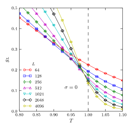
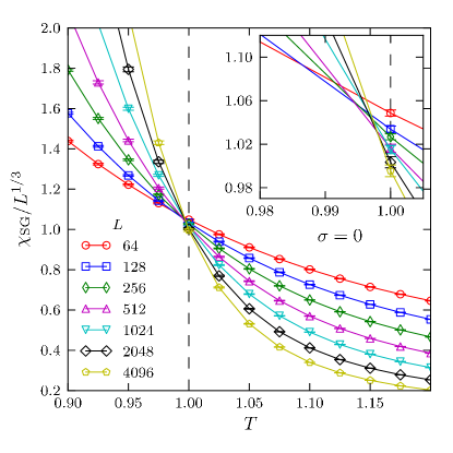
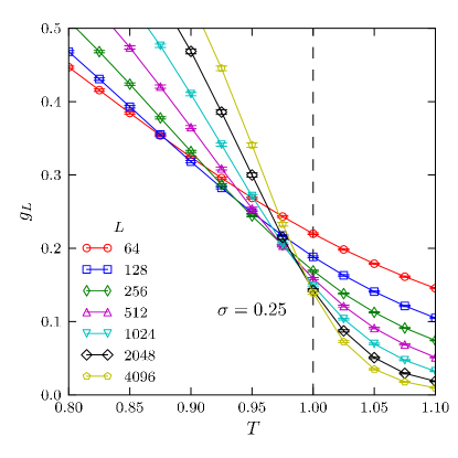
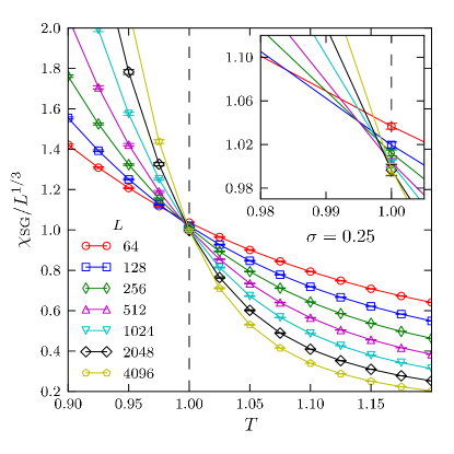
Figure 1: (Color online) Data for the the scaled spin glass susceptibility and the Binder ratio for the undiluted model with $\sigma=0$, the SK model, (top), and the undiluted model with $\sigma=0.25$ (bottom). The dashed vertical line shows the exact value of the transition temperature ($T_{c}=1$) for the SK model.

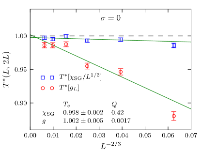
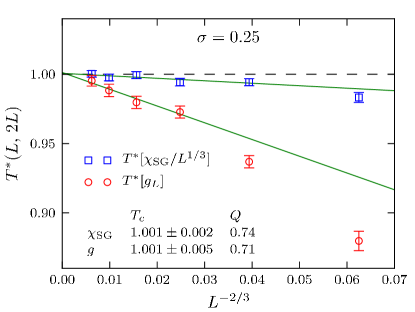
Figure 2: (Color online) Results for the intersection temperatures for the SK model (left) and the undiluted $\sigma=0.25$ model (right).

We focus on moments of the spin glass order parameter $q$ where

$$q={1\over L}\,\sum_{i}S_{i}^{(1)}S_{i}^{(2)}\,,$$ (19)

in which “$(1)$” and “$(2)$” refer to two independent copies of the system with the same interactions. Of particular interest are the spin glass susceptibility

$$\chi_{SG}=L\langle q^{2}\rangle\,,$$ (20)

and the Binder ratio

$$g={1\over 2}\left(3-{[\langle q^{4}\rangle]_{\rm av}\over[\langle q^{2}\rangle]_{\rm av}^{2}}\right)\,.$$ (21)

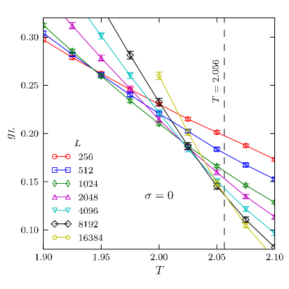
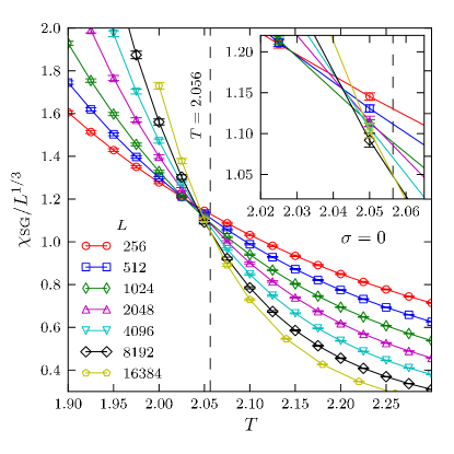
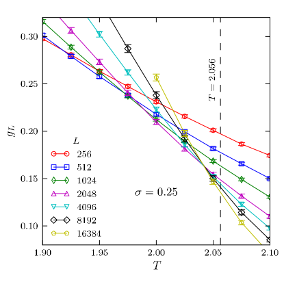
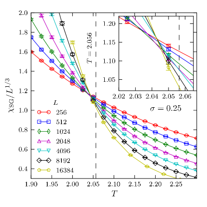
Figure 3: (Color online) Data for the the scaled spin glass susceptibility and the Binder ratio for the Viana-Bray model, i.e. the diluted model with $\sigma=0$ (top), and the diluted model with $\sigma=0.25$ (bottom). The dashed vertical line shows the transition temperature for the Viana-Bray model obtained from Eq. (12) of the text.

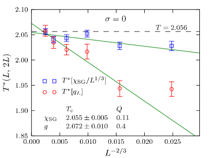
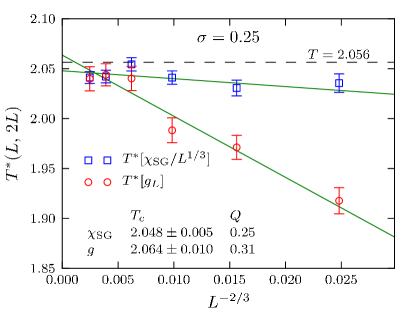
Figure 4: (Color online) Results for the intersection temperatures for the Viana-Bray model (left) and the diluted model with $\sigma=0.25$ (right).

Since the Binder ratio is dimensionless, its finite-size scaling (FSS) behavior is simple. We are always in the regime of mean field critical exponents ($0\leq\sigma<2/3$), so it has the form fss

$$g=\widetilde{g}\left(\,(T-T_{c})\,L^{1/3}\right)\,.$$ (22)

The spin glass susceptibility is not dimensionless but, since we are in the mean field regime, its FSS form is also known exactly. It has the form fss

$$\chi_{SG}=L^{1/3}\,\widetilde{\chi}\left(\,(T-T_{c})\,L^{1/3}\right)\,.$$ (23)

One can therefore determine the transition temperature from where the data for $g$ or $\chi_{SG}/L^{1/3}$ for different sizes intersects. However, we shall see that the data does not all intersect at a single temperature, showing that there are corrections to the FSS form in Eqs. (22) and (23). Consider Eq. (23). According to standard finite-size scaling, the spin-glass susceptibility normally varies near the critical point according to Larson et al. (2010)

$$\chi_{SG}(t,L)=L^{a}\left[f(L^{b}t)+L^{-\omega}g(L^{y}t)+\cdots\right]+c_{0}+c_{1}t+\cdots,$$ (24)

where $t=T-T_{c}$, $a=2-\eta\ (=2\sigma-1\ \text{here})$, and $b=1/\nu$. The $L^{-\omega}$ term is the leading singular correction to scaling and $c_{0}$ is the leading analytic correction to scaling. However, in the mean field limit, $\sigma<2/3$, the exponents $a$ and $b$ are independent of $\sigma$Binder et al. (1985); Luijten et al. (1999); Jones and Young (2005) and take the value at $\sigma_{c}$ for all $1/2<\sigma<\sigma_{c}$, i.e. $a=b=1/3$. Furthermore, although the $L^{2\sigma-1}$ term is replaced as the largest term by an $L^{1/3}$ term (due to the presence of a “dangerous irrelevant variable,”cf. Refs. [Binder et al., 1985; Luijten et al., 1999; Jones and Young, 2005]) we expect Larson et al. (2010) this term to not disappear but rather become a correction to scaling. Hence, we replace Eq. (24) by

$$\chi_{SG}(t,L)=L^{1/3}\left[f(L^{1/3}t)+L^{-\omega}g(L^{1/3}t)+\cdots\right]\\ +d_{0}L^{2\sigma-1}hg(L^{1/3}t)+c_{0}+c_{1}t\cdots.$$ (25)

The correction exponent $\omega$ can be obtained in the mean-field regime from the work of Kotliar et al. Kotliar et al. (1983) and is given by $\omega=2-3\sigma$. Hence, in the non-extensive regime, $\sigma<1/2$ the dominant correction to scaling is the constant $c_{0}$.

Adding a constant to the RHS of Eq. (23) it is straightforward to show that the intersection temperature of the data for $\chi_{SG}/L^{1/3}$ for sizes $L$ and $2L$ is given by

$$T^{\star}(L,2L)=T_{c}+{A\over L^{2/3}}+\cdots\,,$$ (26)

where $A$ is a constant and the omitted terms are higher order in $1/L$. We expect that the intersection temperatures for the data for $g$ have the same form. We shall use Eq. (26) to determine $T_{c}$ for the models studied.

IV Results

We first present our results for the undiluted model. Data for the the scaled spin glass susceptibility and the Binder ratio are shown in Fig. 1. The top part is for the SK model, $\sigma=0$, and the bottom part is for the undiluted model with $\sigma=0.25$. One sees large corrections to scaling for the Binder ratio (the left-hand figures) but much smaller corrections for the scaled spin glass susceptibility (the right-hand figures). The inset enlarges the region of the intersections for the latter data.

Figure 2 shows values for the intersection temperature. These were determined by interpolation using cubic splines, and error bars computed by a jackknife analysis. For both values of $\sigma$ the data extrapolates to a value of 1, the exact value for the SK model, (with very small errors). The quality of the fit, as represented by the goodness of fit parameter $Q$ Press et al. (2007), is satisfactory except for the Binder ratio data for the SK model. We don’t have a good explanation for this, except perhaps that multiple corrections to scaling are significant for the range of sizes studied. In any case we note that the result $T_{c}=1$ for the SK model is rigorously correct. The result that $T_{c}=1$ also for $\sigma=0.25$, at the midpoint of the non-extensive region, provides strong evidence for the claim of Mori Mori that all models in the non-extensive region are identical to the SK model. While it would be useful to check this also in the space glass phase below $T_{c}$, such simulations would be difficult because relaxation times increase dramatically at low $T$ and so the range of sizes that could be studied would be much more limited than in the data presented here.

The corresponding results for the diluted model for $\sigma=0$ and $0.25$ are shown in Figs. 3 and 4. We also performed simulations for $\sigma=0.375$ and show the resulting intersection temperatures in Fig. 5. For $\sigma=0$, the Viana-Bray Viana and Bray (1985) model, the transition temperature is given by Eq. (12) which, for $z=6$ taken here, gives the result in Eq. (13). In Fig. 3 we again see that corrections to scaling are larger for the Binder ratio than for the scaled spin glass susceptibility. The intersection temperatures all extrapolate to the exact value for $\sigma=0$ within statistical uncertainty.

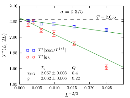
Figure 5: (Color online) Results for the intersection temperatures for the diluted model with $\sigma=0.375$.

V Summary and Conclusions

We have performed Monte Carlo simulations to investigate the transition temperature of one-dimensional Ising spin glasses, both undiluted and diluted, for several values of $\sigma$ in the non-extensive regime $0\leq\sigma<1/2$. For the undiluted model we studied two values of $\sigma$, $\sigma=0$ and $\sigma=0.25$. For $\sigma=0.25$, which lies in the middle of the non-extensive regime, we find that the transition temperature agrees to high precision with the exact solution of the SK model. As a check, we also simulated the $\sigma=0$ case, obtaining results consistent with the exact SK model result, though there seem to be multiple corrections to FSS for some of the data.

For the diluted model we studied three values of $\sigma$: $\sigma=0$, which corresponds to the Viana-Bray model, $\sigma=0.25$, which lies in the middle of the non-extensive regime, and $\sigma=0.375$. In all cases we found the transition temperature to be consistent with the exact solution of the Viana-Bray model; all results are within $\sim 1.5$ standard deviations.

To conclude, our results provide confirmation of the proposal Mori that the behavior of (undiluted) spin glasses everywhere in the non-extensive regime is identical to that of the SK model. We have also proposed that an analogous result applies to diluted spin glass models, and provided numerical evidence for this too.

Appendix A Spherical Approximation for the ferromagnet

For the infinite-range ferromagnet, the interaction $J_{ij}$ is equal to $1/(N-1)$ for $i\neq j$ and 0 for $i=j$. This fixes $T_{c}=1$. The Fourier transform of this interaction is given by

$$J(k)=\delta_{k,0}-{1\over N}\,,$$ (27)

so only the $k=0$ mode contributes to the transition.

For a power-law decay of the interactions in the non-extensive regime ($0<\sigma<1$), on dimensional grounds there is a singular piece which diverges like $k^{\sigma-1}$ for $k\to 0$. Furthermore the interactions have to be multiplied by a number of order $N^{\sigma-1}$ in order to satisfy the condition $T_{c}^{MF}=\sum_{j}J_{ij}=1$. Hence, roughly speaking, we have

$$J(k)\propto\left(k\,N\right)^{\sigma-1}\,,$$ (28)

where we note that $k\equiv k_{n}=2\pi n/L,\ (n=0,1,2,\cdots)$. (For $n=0,J(0)$ does not actually diverge but will be comparable to $J(k_{1})$). Hence other long wavelength modes, in addition to $k=0$, are now significant. However, we shall now see that there are not enough of them to change the value of $T_{c}$ from that of $T_{c}^{MF}\ (=1)$.

We will do this by considering the “spherical approximation” Berlin and Kac (1952). in which we reexpress the problem as a Gaussian one, with “soft” spins $\phi_{i}$ which take values from $-\infty$ to $\infty$, and a Hamiltonian

$$\mathcal{H}_{\text{Gauss}}={1\over 2}\sum_{i,j}\,\left(\mu\delta_{ij}-J_{ij}\right)\,\phi_{i}\phi_{j}\,,$$ (29)

where $\mu$ is a Lagrange multiplier whose value is chosen to enforce the length constraint

$$\langle\phi_{i}^{2}\rangle=1\,.$$ (30)

It turns out the the spherical approximation is exact for an $m$-component model in the limit $m\to\infty$ Stanley (1968). Fourier transforming Eq. (30) and doing the Gaussian integrals gives

$${1\over T}={1\over L}\sum_{k}{1\over\mu-J(k)}\,.$$ (31)

The transition occurs when the denominator vanishes at $k=0$, i.e. when $\mu=J(0)$ and so

$${1\over T_{c}^{\text{spher}}}={1\over L}\sum_{k}{1\over J(0)-J(k)}\,.$$ (32)

It is interesting to compare this with the mean field result, $T_{c}=\sum_{j}J_{ij}=J(0)$. Since $J_{ii}=(1/L)\sum_{k}J(k)=0$ we can rewrite the mean field transition temperature as

$$T_{c}^{MF}={1\over L}\sum_{k}\left[\,J(0)-J(k)\,\right]\,.$$ (33)

Thus, whereas in mean field theory, $T_{c}$ is equal to the average of $J(0)-J(k)$, in the spherical approximation $1/T_{c}$ is equal to the average of the inverse of this.

For the infinite range model, where $J(k)$ is given by Eq. (27) and only the $k=0$ mode contributes, the spherical result agrees with the mean field result (consistent with the MF result being exact for this model).

We now estimate $T_{c}$ from the spherical approximation, Eq. (32), for the power-law model, where $J(k)$ varies like Eq. (28). Because we normalize the interactions to $J(0)=1$, we can include an extra factor of $J(0)$ and expand in powers of $J(k)/J(0)$, i.e.

$${1\over T_{c}^{\text{spher}}} ={1\over L}\sum_{k}{1\over 1-J(k)/J(0)}\,$$ (34a)

$$={1\over L}\sum_{k}\left[1+{J(k)\over J(0)}+\left({J(k)\over J(0)}\right)^{2}+\cdots\right]$$ (34b)

$$=1+{1\over L}\sum_{k}\left[\left({J(k)\over J(0)}\right)^{2}+\cdots\right]$$ (34c)

$$=1+{\sum_{j}J_{ij}^{2}\over\left(\sum_{j}J_{ij}\right)^{2}}+\cdots\,,$$ (34d)

where in Eq. (34c) we used that $\sum_{k}J(k)=0$. In Eq. (34d) we have $\sum_{j}J_{ij}\propto L^{1-\sigma}$ while $\sum_{j}J_{ij}^{2}=L^{1-2\sigma}\,(0\leq\sigma<1/2),\sum_{j}J_{ij}^{2}=\text{const.}\,(1/2<\sigma<1)$. Hence the leading correction term in Eq. (34d) vanishes everywhere in the non-extensive regime.

To conclude, in this appendix we have given a suggestive argument as to why $T_{c}$ for the ferromagnet is given exactly by the mean field value everywhere in the non-extensive regime. It is therefore also plausible that other properties are also identical to those of mean field theory (i.e. the infinite-range model.)

References

- Boettcher (2005) S. Boettcher, Phys. Rev. Lett. 95, 197205 (2005).
- Dyson (1969) F. Dyson, Communications in Mathematical Physics 12, 212 (1969).
- Dyson (1971) F. Dyson, Communications in Mathematical Physics 21, 269 (1971).
- Kotliar et al. (1983) G. Kotliar, P. W. Anderson, and D. L. Stein, Phys. Rev. B 27, 602 (1983).
- Katzgraber and Young (2005) H. G. Katzgraber and A. P. Young, Phys. Rev. B 72, 184416 (2005).
- Katzgraber et al. (2009) H. G. Katzgraber, D. Larson, and A. P. Young, Phys. Rev. Lett 102, 177205 (2009), eprint (arXiv:0812:0421).
- Leuzzi et al. (2008) L. Leuzzi, G. Parisi, F. Ricci-Tersenghi, and J. J. Ruiz-Lorenzo, Phys. Rev. Lett 101, 107203 (2008).
- Moore (2010) M. A. Moore, Phys. Rev. B 82, 014417 (2010).
- Leuzzi et al. (2009) L. Leuzzi, G. Parisi, F. Ricci-Tersenghi, and J. J. Ruiz-Lorenzo, Phys. Rev. Lett 103, 267201 (2009).
- Bray et al. (1986) A. J. Bray, M. A. Moore, and A. P. Young, Phys. Rev. Lett. 56, 2641 (1986), URL http://link.aps.org/doi/10.1103/PhysRevLett.56.2641.
- Larson et al. (2010) D. Larson, H. G. Katzgraber, M. A. Moore, and A. P. Young, Phys. Rev. B 81, 064415 (2010), eprint (arXiv:0908.2224).
- Sherrington and Kirkpatrick (1975) D. Sherrington and S. Kirkpatrick, Phys. Rev. Lett. 35, 1792 (1975).
- Cannas et al. (2000) S. Cannas, A. de Magalhães, and F. Tamarit, Phys. Rev. B 61, 11521 (2000).
- Campa et al. (2000) A. Campa, A. Giasanti, and D. Moroni, Phys. Rev. E 62, 303 (2000).
- (15) T. Mori, (arXiv:1106.4920).
- Viana and Bray (1985) L. Viana and A. J. Bray, J. Phys. C 18, 3037 (1985).
- Katzgraber and Young (2003) H. G. Katzgraber and A. P. Young, Phys, Rev. B 67, 134410 (2003).
- Hukushima and Nemoto (1996) K. Hukushima and K. Nemoto, J. Phys. Soc. Japan 65, 1604 (1996), eprint (arXiv:cond-mat/9512035).
- (19) For a discussion of how finite-size scaling is modified in the region of mean-field exponents, see for example Refs. Brézin (1982); Brézin and Zinn-Justin (1985); Binder et al. (1985); Luijten et al. (1999); Jones and Young (2005).
- Binder et al. (1985) K. Binder, M. Nauenberg, V. Privman, and A. P. Young, Phys. Rev. B 31, 1498 (1985).
- Luijten et al. (1999) E. Luijten, K. Binder, and H. W. J. Blöte, Eur. Phys. J. B 9, 289 (1999).
- Jones and Young (2005) J. L. Jones and A. P. Young, Phys. Rev. B 71, 174438 (2005), eprint (arXiv:cond-mat/0412150).
- Press et al. (2007) W. H. Press, S. A. Teukolsky, W. T. Vetterling, and B. P. Flannery, Numerical Recipes in C++ (Cambridge University Press, Cambridge, 2007), 3rd ed.
- Berlin and Kac (1952) T. H. Berlin and M. Kac, Phys. Rev. 86, 821 (1952), URL http://link.aps.org/doi/10.1103/PhysRev.86.821.
- Stanley (1968) H. E. Stanley, Phys. Rev. 176, 718 (1968), URL http://link.aps.org/doi/10.1103/PhysRev.176.718.
- Brézin (1982) E. Brézin, J. Phys. (Paris) 43, 15 (1982).
- Brézin and Zinn-Justin (1985) E. Brézin and J. Zinn-Justin, Nucl. Phys. B 257, 867 (1985).