Full Counting Statistics for Orbital-Degenerate Impurity Anderson Model
with Hund’s Rule Exchange Coupling

Abstract

We study nonequilibrium current fluctuations through a quantum dot, which includes a ferromagnetic Hund’s rule coupling $J$, in the low-energy Fermi liquid regime using the renormalized perturbation theory. The resulting cumulant for the current distribution in the particle-hole symmetric case shows that spin-triplet and spin-singlet pairs of quasiparticles are formed in the current due to the Hund’s rule coupling and these pairs enhance the current fluctuations. In the fully screened higher-spin Kondo limit, the Fano factor takes a value $F_{b}=(9M+6)/(5M+4)$ determined by the orbital degeneracy $M$. We also investigate the crossover between the small and large $J$ limits in the two-orbital case $M=2$, using the numerical renormalization group approach.

The experimental study of electron transport in mesoscopic devices, subject to applied bias voltages, has provided a new way of investigating interelectron many-body effects Grobis et al. (2008); Hershfield et al. (1991); Oguri (2001). For example, the theoretical prediction that the Kondo correlation on the nonequilibrium currents through quantum dots leads to an enhancement of the shot noise in these systems Sela et al. (2006); Golub (2006); Mora et al. (2009); Fujii (2010) has stimulated subsequent experiments Zarchin et al. (2008); Delattre et al. (2009); Yamauchi et al. (2011).

A deeper understanding of nonequilibrium transport in these systems can be obtained from the calculation of the current distribution function, the higher order cumulants beyond averaged current, and the noise power. These can be calculated from the cumulant generating function (CGF) for nonequilibrium transport. This quantity, however, is difficult to calculate when many-body effects have to be taken into account. A recent development has been the calculation of the current probability distribution for quantum dot in the Kondo regime Gogolin and Komnik (2006a); Schmidt et al. (2007); Sakano et al. (2011) using the general formulation of the full counting statistics (FCS) Bagrets et al. (2006); Esposito et al. (2009). It was shown that quasiparticle singlet pairs carry a charge $2e$ in the backscattering current due to the Kondo correlation and that these enhance the nonequilibrium current fluctuations.

In this Letter, we investigate the FCS for an orbital-degenerate impurity Anderson model as a prototype model to examine the effects of both the Hund’s rule and Kondo correlations and, hence, to deduce the time-averaged current and shot noise. These have been experimentally investigated in vertical dots, carbon nanotubes, and double dots Sasaki et al. (2004); Delattre et al. (2009); Hübel et al. (2008). Using the renormalized perturbation theory (RPT) Hewson (1993), we calculate the zero-temperature CGF up to third order in applied bias voltage for arbitrary strength of the interactions at the dot site in the low-energy Fermi-liquid regime. We show that the Hund’s rule correlation gives rise to spin-triplet pairs and spin-singlet pairs of quasiparticles carrying charge $2e$ in the nonequilibrium current, which characterize the shot noise and higher order cumulants at low energies.

Model.— Let us consider transport through a correlated dot described by an orbital-degenerate impurity Anderson model ${\cal H}_{A}={\cal H}_{0}+{\cal H}_{T}+{\cal H}_{I}$ with

$${\cal H}_{0} = \sum_{k\alpha m\sigma}\varepsilon_{k\alpha}c_{k\alpha m\sigma}^{\dagger}c_{k\alpha m\sigma}+\sum_{m\sigma}\epsilon_{d}\,n_{dm\sigma},$$ (1)

$${\cal H}_{T} = \sum_{k\alpha m\sigma}\left(v_{\alpha}d_{m\sigma}^{\dagger}c_{k\alpha m\sigma}+\mbox{H.c.}\right),$$ (2)

$${\cal H}_{I} = U\sum_{m}n_{dm\uparrow}n_{dm\downarrow}+W\sum_{m>m^{\prime},\sigma\sigma^{\prime}}n_{dm\sigma}n_{dm^{\prime}\sigma^{\prime}}$$ (3)

$$\quad+2J\sum_{m>m^{\prime}}{\bm{S}}_{dm}\cdot{\bm{S}}_{dm^{\prime}}.$$

Here, $d_{m\sigma}$ annihilates an electron in the dot level $\epsilon_{d}$ with orbital $m=1,2,\cdots,M$ and spin $\sigma$, and $c_{k\alpha m\sigma}$ annihilates a conduction electron with moment $k$, orbital $m$, and spin $\sigma$ in lead $\alpha=L,R$. Interactions $U$, $W(0\leq W\leq U)$, and $J(\leq 0)$ are the intra- and interorbital Coulomb repulsion, and Hund’s rule coupling, respectively. $n_{dm\sigma}$ is the number of electron in the dot level with orbital $m$ and spin $\sigma$, and ${\bm{S}}_{dm}$ is the spin operator of electrons in orbital $m$ of the dot. The intrinsic level width of the dot levels owing to tunnel coupling $v_{\alpha}$ is given by $\Gamma=\sum_{\alpha}\pi\rho_{\rm c}v_{\alpha}^{2}$ with the density of state of the conduction electrons $\rho_{\rm c}$. The two-orbital case ($M=2$) has been experimentally realized in such systems as vertical dots, carbon-nanotube dots, and four-terminal double-dots Sasaki et al. (2004); Delattre et al. (2009); Hübel et al. (2008). For simplicity, the symmetric lead-dot coupling $v_{L}=v_{R}$ and the particle-hole symmetry $\epsilon_{d}=-U/2-(M-1)W$ are assumed. The chemical potentials of the leads $\mu_{L/R}=\pm V/2$, satisfying $\mu_{L}-\mu_{R}=V(>0)$, are measured relative to the Fermi level defined at zero voltage $V=0$. We take units with $\hbar=k_{\rm B}=e=1$ throughout this Letter.

Full counting statistics.— The probability distribution $P(q)$ of the transferred charge $q$ across the dot during a time interval ${\cal T}$ can provide the current correlation functions to all orders. In order to treat them systematically, we calculate the CGF $\ln\chi\left(\lambda\right)=\ln\sum_{q}e^{i\lambda q}P(q)$ in the Keldysh formulation Levitov and Reznikov (2004): $\ln\chi\left(\lambda\right)=\ln\left\langle T_{C}S_{C}^{\lambda}\right\rangle$ where $S_{C}^{\lambda}=T_{C}\exp\left\{-i\int_{C}dt\left[{\cal H}_{T}^{\lambda}(t)+{\cal H}_{I}(t)\right]\right\}$ is the time evolution operator for an extended Hamiltonian ${\cal H}_{A}^{\lambda}={\cal H}_{0}+{\cal H}_{T}^{\lambda}+{\cal H}_{I}$, $C$ is the Keldysh contour along $[t:-{\cal T}/2\to+{\cal T}/2\to-{\cal T}/2]$, $T_{C}$ is the contour-ordering operator, and $\lambda$ is the counting field. Here, ${\cal H}_{T}^{\lambda}$ is given by

$${\cal H}_{T}^{\lambda}=\sum_{km\sigma}\left[v_{L}e^{i\lambda(t)/2}d_{m\sigma}^{\dagger}c_{kLm\sigma}+v_{R}d_{m\sigma}^{\dagger}c_{kRm\sigma}+\mbox{H.c.}\right],$$ (4)

with the contour-dependent counting-field defined by $\lambda(t)\equiv\lambda_{\mp}=\pm\lambda$ for the forward and backward paths labeled by “$-$” and “$+$” respectively.

To calculate the CGF, we use Komnik and Gogolin’s procedure Gogolin and Komnik (2006b) outlined below. First, a more general function $\chi(\lambda_{-},\lambda_{+})$ is introduced. It is basically given by $\ln\left\langle T_{C}S_{C}^{\lambda}\right\rangle$ but $\lambda_{\mp}$ is formally treated as an independent variable assigned for each contour. For the long time limit ${\cal T}\to\infty$ where the switching effect is negligible, the general CGF is proportional to ${\cal T}$. Then, the derivative of the CGF with respect to $\lambda_{-}$ is given in terms of Green’s functions as

$$\frac{d}{d\lambda_{-}}\ln\chi(\lambda_{-},\lambda_{+})$$

$$\quad=-i{\cal T}\frac{v_{L}^{2}}{2}\sum_{km\sigma}\int\frac{d\omega}{2\pi}\left[e^{-i\bar{\lambda}/2}G_{d}^{\lambda-+}\left(\omega\right)g_{kL}^{0+-}\left(\omega\right)\right.$$

$$\quad\qquad\qquad\qquad\qquad-\left.e^{i\bar{\lambda}/2}g_{kL}^{0-+}\left(\omega\right)G_{d}^{\lambda+-}\left(\omega\right)\right],$$ (5)

with $\bar{\lambda}\equiv\lambda_{-}-\lambda_{+}$. $g_{k\alpha}^{0-+}(\omega)=i2\pi\delta(\omega-\varepsilon_{k\alpha})f_{\alpha}(\omega)$ and $g_{k\alpha}^{0+-}(\omega)=-i2\pi\delta(\omega-\varepsilon_{k\alpha})[1-f_{\alpha}(\omega)]$ are the lesser and greater parts of the Green’s function for electrons in lead $\alpha$, respectively, with the Fermi distribution function $f_{\alpha}(\omega)=[e^{(\omega-\mu_{\alpha})/T}+1]^{-1}$. For the long time limit ${\cal T}\to\infty$, the dot Green’s function is defined as $G_{d}^{\lambda\,\nu\nu^{\prime}}(\omega)=-i\int d(t-t^{\prime})e^{i\omega(t-t^{\prime})}\langle T_{C}d_{m\sigma}(t_{\nu})d_{m\sigma}^{\dagger}(t^{\prime}_{\nu^{\prime}})\rangle_{\lambda_{-},\lambda_{+}}$. $\nu$ and $\nu^{\prime}$ are the labels for the two Keldysh contours. Here, we use a notation $\langle A(t)\rangle_{\lambda_{-},\lambda_{+}}\equiv\left\langle T_{C}S_{C}^{\lambda}A(t)\right\rangle\big{/}\chi(\lambda_{-},\lambda_{+})$ which represents an expectation for Hamiltonian ${\cal H}_{A}^{\lambda}$. Once $\ln\chi(\lambda_{-},\lambda_{+})$ is computed, the statistics are recovered from $\ln\chi(\lambda)=\ln\chi(\lambda,-\lambda)$.

Renormalized perturbation theory.— To calculate the Keldysh Green’s function with finite $\lambda$ at low energies, we use the RPT outlined below Hewson (1993); Nishikawa et al. (2010); Oguri (2005). The basic parameters that specify the impurity Anderson model ${\cal H}_{A}$ are $\epsilon_{d}$, $\Gamma$, $U$, $W$, and $J$. Correspondingly, the low-energy excitations can be characterized by the renormalized parameters for the quasiparticles: dot-level $\widetilde{\epsilon}_{d}=z\left[\epsilon_{d}+\Sigma_{d}^{r}(0)\right]$, level width $\widetilde{\Gamma}=z\Gamma$, where $\Sigma_{d}^{r}(\omega)$ is the self-energy of the retarded Green’s function for the dot state $G_{d}^{r}(\omega)=[\omega-\epsilon_{d}+i\Gamma-\Sigma_{d}^{r}(\omega)]^{-1}$, $z=[1-\partial\Sigma_{d}^{r}(\omega)/\partial\omega|_{\omega=0}]^{-1}$ is the wave function renormalization factor. Here, $\widetilde{\Gamma}$ corresponds to the characteristic energy scale, namely, the Kondo temperature $T_{K}=\pi\widetilde{\Gamma}/4$. The quasiparticle interactions $\tilde{U},\tilde{W}$ and $\tilde{J}$ are defined in terms of the local full four-vertex for the scattering of the electrons, $\Gamma_{m_{3}\sigma_{3};m_{4}\sigma_{4}}^{m_{1}\sigma_{1};m_{2}\sigma_{2}}(\omega_{1},\omega_{2},\omega_{3},\omega_{4})$ taken at zero frequency $\omega_{i}=0$ (see Ref. Nishikawa et al., 2010). In this Letter, we choose the renormalized parameters defined at the equilibrium ground state. Then, the replacement of the bare parameters with the renormalized ones gives the leading terms of an effective Hamiltonian corresponding to the low-energy fixed point of the numerical renormalization group (NRG). The renormalized parameters can be related to the enhancement factors of spin, orbital and charge susceptibilities; $z\widetilde{\chi}_{\rm s}=1+\widetilde{\rho}_{d}(0)\left[\widetilde{U}-(M-1)\widetilde{J}\right],z\widetilde{\chi}_{\rm orb}=1+\widetilde{\rho}_{d}(0)\left[2\widetilde{W}-\widetilde{U}\right],z\widetilde{\chi}_{\rm c}=1-\widetilde{\rho}_{d}(0)\left[\widetilde{U}+2(M-1)\widetilde{W}\right],$ with the renormalized density of state $\widetilde{\rho}_{d}(\omega)=(\widetilde{\Gamma}/\pi)/[(\omega-\widetilde{\epsilon}_{d})^{2}+\widetilde{\Gamma}^{2}]$, and also to the Friedel sum rule $\pi\langle n_{dm\sigma}\rangle=\cot^{-1}\left(\widetilde{\epsilon}_{d}/\widetilde{\Gamma}\right)$. These relations enable one to deduce the value of renormalized parameters in some special limits. For instance, the renormalized dot level in the particle-hole symmetric case is situated at the Fermi energy $\tilde{\epsilon}_{d}=0$. We can also evaluate the renormalized parameters for dots with two orbitals $(M=2)$ with the NRG approach Nishikawa et al. (2010).

The nonequilibrium perturbation theory in powers of $U,W$ and $J$ can be reorganized as an expansion with respect to the renormalized interactions $\widetilde{U},\widetilde{W}$, and $\widetilde{J}$ by taking the free quasiparticle Green’s function of the form

$$\widetilde{g}_{d}^{\lambda--}(\omega) = \left[\omega-\widetilde{\epsilon}_{d}-i\widetilde{\Gamma}+i\widetilde{\Gamma}\textstyle\sum_{l}f_{l}\right]\Big{/}{\cal D},$$

$$\widetilde{g}_{d}^{\lambda-+}(\omega) = \left[i\widetilde{\Gamma}e^{i\bar{\lambda}/2}f_{L}+i\widetilde{\Gamma}f_{R}\right]\Big{/}{\cal D},$$

$$\widetilde{g}_{d}^{\lambda+-}(\omega) = -\left[i\widetilde{\Gamma}e^{-i\bar{\lambda}/2}\left(1-f_{L}\right)+i\widetilde{\Gamma}\left(1-f_{R}\right)\right]\Big{/}{\cal D},$$

$$\widetilde{g}_{d}^{\lambda++}(\omega) = \left[-\omega+\widetilde{\epsilon}_{d}-i\widetilde{\Gamma}+i\widetilde{\Gamma}\textstyle\sum_{l}f_{l}\right]\Big{/}{\cal D},$$ (6)

with ${\cal D}=\left(\omega-\widetilde{\epsilon}_{d}\right)^{2}+\widetilde{\Gamma}^{2}+\widetilde{\Gamma}^{2}\left(e^{i\bar{\lambda}/2}-1\right)\left(1-f_{R}\right)f_{L}$ as the zero-order propagator Oguri (2005). With this approach, the exact form of the Green’s function can be calculated at low energies up to terms of order $\omega^{2}$, $V^{2}$, and $T^{2}$.

We calculate the Green’s function ${\bm{G}}_{d}^{\lambda}(\omega)$ under a finite counting field through the Dyson equation

$${\bm{G}}_{d}^{\lambda}(\omega)=z\widetilde{{\bm{G}}}_{d}^{\lambda}(\omega)=z\left[{\widetilde{{\bm{g}}}_{d}^{\lambda}(\omega)}^{-1}-\widetilde{{\bm{\Sigma}}}_{d}^{\lambda}(\omega)\right]^{-1}.$$ (7)

The renormalized self-energy at $T=0$ up to $\omega^{2},\omega V$, and $V^{2}$ in the particle-hole symmetric case can be calculated in the second order perturbation in the three renormalized interactions as

$$\widetilde{{\bm{\Sigma}}}_{d}^{\lambda}(\omega)=\frac{-i}{8\widetilde{\Gamma}}\,\widetilde{\cal I}\left[\begin{array}[]{cc}A(\omega,V)&B(\omega,V)\\ -B^{\ast}(-\omega,-V)&A(\omega,V)\end{array}\right],$$ (10)

with

$$A(\omega,V) = \left[a\left(\omega,3V/2\right)+3\,a\left(\omega,V/2\right)\right.$$ (11)

$$\qquad+\left.3\,a\left(\omega,-V/2\right)+a\left(\omega,-3V/2\right)\right],$$

$$B(\omega,V) = \left[e^{-i\bar{\lambda}/2}b\left(\omega,3V/2\right)+3b\left(\omega,V/2\right)\right.$$ (12)

$$\ \left.+3e^{i\bar{\lambda}/2}b\left(\omega,-V/2\right)+e^{i\bar{\lambda}}b\left(\omega,-3V/2\right)\right],$$

$$\widetilde{\cal I} = \tilde{u}^{2}+2(M-1)\left(\tilde{w}^{2}+3\tilde{j}^{2}/4\right)$$ (13)

Here, $a(\omega,x)=-\frac{1}{2}(\omega-x)^{2}\mbox{sgn}(-\omega+x)$, $b(\omega,x)=(\omega-x)^{2}\theta(-\omega+x)$, and $\tilde{u}\equiv\widetilde{U}/(\pi\widetilde{\Gamma}),\tilde{w}\equiv\widetilde{W}/(\pi\widetilde{\Gamma})$ and $\tilde{j}\equiv\widetilde{J}/(\pi\widetilde{\Gamma})$. For $\lambda=0$, it corresponds to an extension of Ref. Oguri, 2001 to the orbital-degenerate Anderson model.

Results and discussion.— Integrating Eq. (5) with respect to $\lambda_{-}$, the CGF is calculated at $T=0$ up to $V^{3}$, as $\ln\chi(\lambda)={\cal F}_{0}+{\cal F}_{1}+{\cal F}_{2}$ with

$${\cal F}_{0} = \frac{2M{\cal T}}{2\pi}\int_{-V/2}^{V/2}d\omega\ln\left[1+T(\omega)\left(e^{i\lambda}-1\right)\right],$$ (14)

$${\cal F}_{1} = {\cal T}P_{b1}\left(e^{-i\lambda}-1\right),\quad{\cal F}_{2}={\cal T}P_{b2}\left(e^{-i2\lambda}-1\right).$$ (15)

Here, ${\cal F}_{0}$ describes free-quasiparticle tunneling via the renormalized level with transmission probability $T(\omega)=\widetilde{\Gamma}^{2}/(\omega^{2}+\widetilde{\Gamma}^{2})$, which carries single charge $e$. ${\cal F}_{1}$ and ${\cal F}_{2}$ represent the scattering process due to the residual interactions $\widetilde{U}$, $\widetilde{W}$, and $\widetilde{J}$. From the coefficient of the counting field in ${\cal F}_{1}$ and ${\cal F}_{2}$, it is clear that $P_{b1}=\frac{M}{12\pi}\tilde{\cal I}\frac{V^{3}}{\widetilde{\Gamma}^{2}}$ and $P_{b2}=\frac{M}{6\pi}\tilde{\cal I}\frac{V^{3}}{\widetilde{\Gamma}^{2}}$ are the probabilities of the single- and paired-quasiparticle backscattering processes carrying charge $e$ and $2e$, respectively. Then, the $n$th-order cumulant ${\cal C}_{n}=(-i)^{n}\frac{d^{n}}{d\lambda^{n}}\ln\chi(\lambda)$ is readily derived as

$${\cal C}_{n}={\cal T}\left[I_{u}\delta_{1n}+(-1)^{n}(P_{b0}+P_{b1}+2^{n}P_{b2})\right],$$ (16)

where $I_{u}=2MV/(2\pi)$ is the linear-response current and $P_{b0}=\frac{M}{12\pi}\frac{V^{3}}{\widetilde{\Gamma}^{2}}$ represents the probability of the single-quasiparticle backscattering processes due to the renormalized level. Especially, the factor $2^{n}$ characterizing cumulant of interacting electrons (16) indicates the existence of spin-singlet, orbital-singlet, and spin-triplet pairs of quasiparticles in the nonequilibrium current. Equation (16) generalizes the previous results of the cumulant for the SU($2M$) case where $U=W$ and $J=0$ Gogolin and Komnik (2006a); Schmidt et al. (2007); Sakano et al. (2011). In the present result, the Hund’s coupling enters through the $P_{b1}$ and $P_{b2}$ as well as the Kondo energy scale $\tilde{\Gamma}$. Therefore, it gives rise to the spin-triplet pairs in the current, and also varies the couplings of the spin sector $\tilde{u}$ and the orbital sector $\tilde{w}$, which causes the crossover seen in the current fluctuation as discussed below.

In the series of cumulant ${\cal C}_{n}$, the first two coefficients ${\cal C}_{1}$ and ${\cal C}_{2}$ give time-averaged current $I={\cal C}_{1}/{\cal T}$ and shot noise $S=2{\cal C}_{2}/{\cal T}$, respectively. The higher order ones, ${\cal C}_{n}$ for $n\geq 3$, are determined by these two and are automatically generated by Eq. (16). From these coefficients, the Fano factor of the shot noise for the backscattering current $I_{b}\equiv I_{u}-I$, can be deduced in the form

$$F_{b}\,\equiv\,\frac{S}{2I_{b}}\,=\,\frac{1+9\,\widetilde{{\cal I}}}{1+5\,\widetilde{{\cal I}}}.$$ (17)

This is an important result of this Letter . The Fano factor $F_{b}$ determines the effective charges of the backscattering current Sela et al. (2006). Our results, Eq.  (17) with (13), show that $F_{b}$ also represents the degree of the residual interaction, as the Wilson ratio $R=z\widetilde{\chi}_{\rm s}$ does in the SU(2) case. We examine the value of the Fano factor in some special limits in the following.

First, in the weak coupling limit $u,w,|j|\ll 1$, the renormalized parameters take a form $(\widetilde{u},\widetilde{w},\widetilde{j})\to(u,w,j)$ and $z\to 1-\left(3-\frac{1}{4}\pi^{2}\right)\left[u^{2}+2(M-1)\left(w^{2}+3j^{2}/4\right)\right]$ with scaled interactions $u\equiv U/(\pi\Gamma),w\equiv W/(\pi\Gamma)$, and $j\equiv J/(\pi\Gamma)$. Substituting these into Eq. (17), the result for the second-order perturbation in the bare interactions is produced. In particular, the Fano factor for noninteracting limit $u=w=j=0$ naturally becomes unity which represents single charge transport given by Eq. (14).

In the large Hund’s coupling limit $|j|\gg 1$, the dot state is restricted to the highest spin state, for which we obtain the Kondo coupling ${\cal H}_{K}$ from the Anderson model ${\cal H}_{A}$ in the form

$${\cal H}_{K}=J_{K}\sum_{kk^{\prime}\sigma\sigma^{\prime}m}c_{km\sigma}^{\dagger}{\bm{\sigma}}_{\sigma\sigma^{\prime}}c_{k^{\prime}m\sigma^{\prime}}\cdot{\bm{S}}_{d}$$ (18)

with $J_{K}=4(v_{L}^{2}+v_{R}^{2})\left[U-(M-1)J\right]^{-1}$, the Pauli matrix ${\bm{\sigma}}_{\sigma\sigma^{\prime}}$, $c_{km\sigma}=\sum_{\alpha}c_{k\alpha m\sigma}/\sqrt{2}$, and the $S=M/2$ spin operator for the dot-site ${\bm{S}}_{d}$. In this limit, the high spin $S=M/2$ $(\geq 1)$ state is fully screened, and the Wilson ratio becomes $R=2(M+2)/3$ Yoshimori (1976). The charge and orbital fluctuations are suppressed $\widetilde{\chi}_{\rm c}\to 0$ and $\widetilde{\chi}_{\rm orb}\to 0$ in the limit $j\to-\infty$. Therefore, the renormalized parameters take the value $(\widetilde{u},\widetilde{w},\widetilde{j})\to(1,0,-2/3)$. Then, through Eqs. (13) and (17), we find the Fano factor in this limit,

$$F_{b}\to\frac{9M+6}{5M+4}=\frac{9S+3}{5S+2}.$$ (19)

We note that to observe the Fano factor due to the higher-spin Kondo effect in real experiments, Hund’s coupling $J$ is not required to be very large as long as it is larger than the Kondo temperature $J>T_{K}$. The explicit values of the Fano factor in this limit for several $M$ are shown in Table 1. For comparison, the Fano factor in the SU($2M$) Kondo limit $u=w\to\infty,j=0$, $F_{b}\to(M+4)/(M+2)$ Mora et al. (2009); Sakano et al. (2011), is also shown in Table 1.

Table 1: The Fano factor $F_{b}={\cal C}_{2}/({\cal T}I_{b})$ in (a) the large Hund’s coupling $j\to-\infty$ or the $S=M/2$ Kondo limit, and (b) the SU($2M$) Kondo limit $u=w\to\infty,j=0$.

$M$	1	2	3	4	$\to\infty$
(a) $S=M/2$ Kondo		12/7	33/19	7/4	$\to 9/5$
(b) SU($2M$) Kondo	5/3	3/2	7/5	4/3	$\to 1$

Increasing orbital degeneracy $M$ in the SU($2M$) Kondo limit, the system approaches the mean-field limit $F_{b}\to 1$ Sakano et al. (2011). In contrast, for large $|j|$, the renormalized interactions $\tilde{u}$, $\tilde{w}$, and $\tilde{j}$ converge to values independent of the orbital degeneracy $M$. As $M$ increases, the number of coupled orbitals with the Hund’s coupling $J$ increases. It results in an enhancement of the spin fluctuations, as seen in the expression of $z\widetilde{\chi}_{\rm s}$ or the interaction factor of the self-energy given in Eq. (13). Therefore, we conclude that the Fano factor increases with $M$, through the enhancement of the quasiparticle-pair scatterings due to the residual Hund’s coupling $\tilde{j}$.

Next, $J$-dependent crossover of the Fano factor for the two-orbital case ($M=2$) is investigated, evaluating the renormalized parameters with the NRG approach. The Fano factor for $u=w$ and $u=3>w$ as a function of Hund’s coupling $j$ are shown in Fig. 1(a)

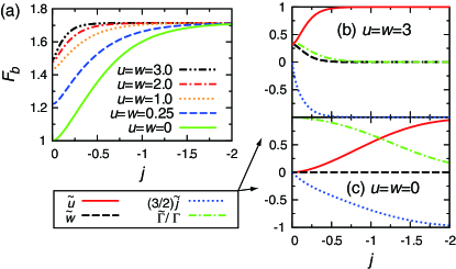
Figure 1: (Color online) (a) The Fano factor for several choices of Coulomb repulsion $u=w$ as a function of scaled Hund’s coupling $j$. (b) The renormalized parameters for $u=w=3$ and (c) $u=w=0$, as a function of $j$.

and Fig. 2(a), respectively.

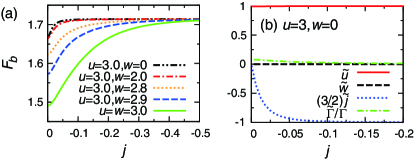
Figure 2: (Color online) (a) The Fano factor for several Coulomb interaction $w(\leq u=3)$ as a function of scaled Hund’s coupling $j$. (b) The renormalized parameters for $(u,w)=(3,0)$ as a function of $j$.

The crossover is observed in the Fano factor around the coupling corresponding to the Kondo temperature $|j|\sim t_{K}\equiv\widetilde{\Gamma}/(4\Gamma)$. At large $|j|$, the Fano factor for any $u\geq w$ converges to a value 12/7 given by Eq. (19), as discussed above. However, at small $|j|$, the values of the Fano factor depend on Coulomb repulsions $u$ and $w$. The Fano factor and the renormalized level-width (or the Kondo temperature) at $j=0$ for several intraorbital Coulomb interaction $u$ as a function of interorbital Coulomb interaction $w$ are shown in Fig. 3 (a) and (b), respectively.

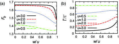
Figure 3: (Color online) (a)The Fano factor and (b) the renormalized level width for no Hund’s coupling $j=0$ and several intraorbital Coulomb repulsions $u$, as a function of interorbital Coulomb repulsions $w(\leq u)$.

With an increase of interorbital Coulomb repulsion $w$, the Fano factor varies from the SU(2) value to the SU(4) value around $(u-w)\sim t_{K}$.

The crossover seen in the Fano factor is a consequence of the behavior of the renormalized parameters, which enter through Eq. (17). Thus, the feature discussed above is also seen in the renormalized parameters, which for $(u,w)=(3,3)$, $(0,0)$, and $(3,0)$ are shown in Figs. 1 (b) and (c), and Fig. 2 (b), respectively, as a function of $j$. Particularly, in Fig. 1 (b), we see a general trend that the spin coupling of the Kondo correlation $\widetilde{u}$ increases, whereas the orbital coupling $\widetilde{w}$ decreases, with increase of the ferromagnetic coupling $-j$. These renormalized parameters converge to the value $(\tilde{u},\tilde{w},\tilde{j})=(1,0,-2/3)$ in the large Hund’s coupling limit. Even for $(u,w)=(0,0)$, the Hund’s coupling enhances the spin coupling $\tilde{u}$ as shown in Fig. 1(c).

Summary.—We have studied the role of the ferromagnetic Hund’s rule coupling on the FCS for the orbital-degenerate Anderson impurity in the particle-hole symmetric case. Using the RPT, we have derived the CGF for nonequilibrium-current distribution. The result is asymptotically exact at low energies and is described by the quasiparticles of the local Fermi liquid. Specifically, the explicit expression of the Fano factor for the shot noise is obtained in the fully screened higher-spin Kondo limit, which depends only on the orbital degeneracy $M$. We have also investigated the crossover between the large and small Hund’s coupling limits in the two-orbital case ($M=2$), using the NRG approach. Furthermore, the CGF indicates that the Hund’s coupling gives rise to singlet and triplet pairs of quasiparticles carrying charge $2e$ in the backscattering current and these correlated charges characterize the current fluctuation through the dot.

R.S. acknowledges Takeo Kato, Yasuhiro Utsumi, Kensuke Kobayashi, Yuma Okazaki, and Satoshi Sasaki for fruitful discussion. This work was supported by the JSPS through its FIRST program, the JSPS Grant-in-Aid for Scientific Research C (No. 23540375) and S (No. 19104007), and MEXT through KAKENHI “Quantum Cybernetics” project and through Project for Developing Innovation Systems.

References

- Grobis et al. (2008) M. Grobis, I. G. Rau, R. M. Potok, H. Shtrikman, and D. Goldhaber-Gordon, Phys. Rev. Lett. 100, 246601 (2008).
- Hershfield et al. (1991) S. Hershfield, J. H. Davies, and J. W. Wilkins, Phys. Rev. Lett. 67, 3720 (1991).
- Oguri (2001) A. Oguri, Phys. Rev. B 64, 153305 (2001).
- Sela et al. (2006) E. Sela, Y. Oreg, F. von Oppen, and J. Koch, Phys. Rev. Lett. 97, 086601 (2006).
- Golub (2006) A. Golub, Phys. Rev. B 73, 233310 (2006).
- Mora et al. (2009) C. Mora, P. Vitushinsky, X. Leyronas, A. A. Clerk, and K. Le Hur, Phys. Rev. B 80, 155322 (2009).
- Fujii (2010) T. Fujii, J. Phys. Soc. Jpn. 79, 044714 (2010).
- Zarchin et al. (2008) O. Zarchin, M. Zaffalon, M. Heiblum, D. Mahalu, and V. Umansky, Phys. Rev. B 77, 241303 (2008).
- Delattre et al. (2009) T. Delattre, C. Feuillet-Palma, L. G. Herrmann, P. Morfin, J.-M. Berroir, G. Fève, B. Plaçais, D. C. Glattli, M.-S. Choi, C. Mora, and T. Kontos, Nat. Phys. 5, 208 (2009).
- Yamauchi et al. (2011) Y. Yamauchi, K. Sekiguchi, K. Chida, T. Arakawa, S. Nakamura, K. Kobayashi, T. Ono, T. Fujii, and R. Sakano, Phys. Rev. Lett. 106, 176601 (2011).
- Gogolin and Komnik (2006a) A. O. Gogolin and A. Komnik, Phys. Rev. Lett. 97, 016602 (2006a).
- Schmidt et al. (2007) T. L. Schmidt, A. Komnik, and A. O. Gogolin, Phys. Rev. B 76, 241307 (2007).
- Sakano et al. (2011) R. Sakano, A. Oguri, T. Kato, and S. Tarucha, Phys. Rev. B 83, 241301 (2011).
- Bagrets et al. (2006) D. Bagrets, Y. Utsumi, D. Golubev, and G. Schön, Fortschr. Phys. 54, 917 (2006).
- Esposito et al. (2009) M. Esposito, U. Harbola, and S. Mukamel, Rev. Mod. Phys. 81, 1665 (2009).
- Sasaki et al. (2004) S. Sasaki, S. Amaha, N. Asakawa, M. Eto, and S. Tarucha, Phys. Rev. Lett. 93, 017205 (2004).
- Hübel et al. (2008) A. Hübel, K. Held, J. Weis, and K. v. Klitzing, Phys. Rev. Lett. 101, 186804 (2008).
- Hewson (1993) A. C. Hewson, Phys. Rev. Lett. 70, 4007 (1993).
- Levitov and Reznikov (2004) L. S. Levitov and M. Reznikov, Phys. Rev. B 70, 115305 (2004).
- Gogolin and Komnik (2006b) A. O. Gogolin and A. Komnik, Phys. Rev. B 73, 195301 (2006b).
- Nishikawa et al. (2010) Y. Nishikawa, D. J. G. Crow, and A. C. Hewson, Phys. Rev. B 82, 115123 (2010).
- Oguri (2005) A. Oguri, J. Phys. Soc. Jpn 74, 110 (2005).
- Note (1) Our calculations can be extended to the particle-hole asymmetric case but the equations are more complicated as the transport coefficients depend also on the order term of the real part of the self-energy Oguri (2001).
- Yoshimori (1976) A. Yoshimori, Prog. Theor. Phys. 55, 67 (1976).