Percolation analysis of force networks in anisotropic granular matter

Abstract

We study the percolation properties of force networks in an anisotropic model for granular packings, the so-called q-model. Following the original recipe of Ostojic et al. [Nature 439 828 (2006)], we consider a percolation process in which forces smaller than a given threshold $f$ are deleted in the network. For a critical threshold $f_{c}$, the system experiences a transition akin to percolation. We determine the point of this transition and its characteristic critical exponents applying a finite-size scaling analysis that takes explicitly into account the directed nature of the q-model. By means of extensive numerical simulations, we show that this percolation transition is strongly affected by the anisotropic nature of the model, yielding characteristic exponents which are neither those found in isotropic granular systems nor those in the directed version of standard percolation. The differences shown by the computed exponents can be related to the presence of strong directed correlations and mass conservation laws in the model under scrutiny.

1 Introduction

Granular media show a peculiar kinetic behavior including the possibility of exhibiting jammed configurations. Jammed assemblies of grains at high densities are not able to explore the phase space but can eventually yield at high drives, for instance under shear stress, like a viscoplastic solid or a complex fluid [1, 2]. Over the last years, experimental observations and numerical simulations of jammed granular media have repeatedly shown the heterogeneous distribution of stress and contact forces in dense packings [3]. Starting from the first studies of weight distributions in bead packs [4, 5], the presence of force chains has been especially emphasized, chains which form an intricate force network structure and are responsible for most of the material’s unusual properties. Force networks in a dense granular packing play the role of the cytoskeleton in a living cell, thus determining its mechanical response and stability. They are also at the core of several important properties of granular media such as friction and wear [6], sound transmission [7], or even electrical transport [8].

Internal stress and contact forces can be determined experimentally, using for example photo-elastic materials, which exhibit stress-induced birefringence. The results obtained from birefringent packings confirm that large forces seem to indeed concentrate along branching-like paths, i.e. force chains or arches. Following some of these measurements, it was argued that a close inspection of contact force properties (for instance, the shape of force probability distributions) could provide new insights regarding the jamming-yielding transition in granular matter [9, 10]. Nevertheless, the distribution of forces alone does not describe the rich topological features observed in experiments nor their potential physical consequences, and complementary methods are thus required for their analysis.

The force network in a granular system is usually defined by the contacts exerted between pairs of particles in the bulk of the system, in such a way that, if particles $i$ and $j$ are in contact, they mutually exert a symmetric force $f_{ij}$ that can also include elastic and/or friction interactions. We can represent these pairwise interactions in terms of a graph or network [11], in which vertices represent the particles, and two vertices are joined by an edge if the respective particles are in contact. This force network can be further characterized as a weighted network, in which each edge has assigned a real value $f_{ij}$, representing the actual value of the force exerted by the vertices (the particles) $i$ and $j$ at the ends of the edge.

Recently, Ostojic et al. [12, 13] proposed a novel way to obtain information about the structure of force networks in static granular matter. The method is formulated in analogy with percolation theory [14, 15] and is based on the scaling properties of clusters of particles connected by relatively large forces. Since each edge carries a force $f_{ij}$, a natural way to visualize the paths that carry the largest weight (arches) is to consider only those edges with a force larger than a given threshold $f$, $f_{ij}>f$, deleting those with $f_{ij}<f$. For small values of $f$, essentially all forces remain in the system, and they form a connected network with a single cluster encompassing all the particles in the system. Upon increasing the value of $f$, the network is expected to break down in subnetworks of connected forces, each representing a path of large weight. Each one of these subnetworks can be understood in terms of clusters in a percolation problem [14]. By analogy with the standard percolation transition, one expects to find a critical percolation threshold $f_{c}$, such that for $f>f_{c}$ the force network is fragmented into a large number of small clusters, while for $f=f_{c}$ a large spanning cluster develops, reaching the boundaries of the system. This analogy with a percolation transition makes it possible to characterize complex contact force networks in terms of a reduced number of critical exponents [15].

In Ref. [12] the percolation transition in contact force networks was first studied by applying a finite-size scaling (FSS) [16] data collapse technique. This technique allows to estimate the value of the percolation threshold $f_{c}$ as well as some exponents related to the divergence of the average cluster size in the infinite network size limit. The remarkable conclusion of this work is that different isotropic models of a dense granular packing seem to exhibit similar percolation exponent values, independently of their microscopic details. Thus these exponents appear to define a robust new universality class for contact force networks, a class which, on the other hand, is different from that of standard percolation.

Many real granular systems, however, are strongly anisotropic; for example, sand piles and silos are driven by the action of gravity, and have therefore a preferred (downwards) direction. The presence of anisotropy should in these other cases be naturally reflected in the contact force network percolation transition, making it in principle more akin to the anisotropic counterpart of percolation, namely directed percolation [17]. In fact, in Ref. [13] (see also [12]) it was observed that anisotropic packing models indeed exhibit a different scaling in their force network percolation transition. The results in Refs. [12, 13] however, were based in the application of an intrinsically isotropic formalism to an anisotropic system, not taking into account, for example, that correlation lengths along different directions might scale differently.

Our purpose in this paper is to fill in this gap, presenting a detailed study of the force network percolation transition in an anisotropic system, performing a direct anisotropic scaling analysis. We focus on the q-model [19], a toy granular model intended to represent the behavior of silos, having a clearly defined preferred direction, in which the weight of the particles is transmitted by virtue of gravity. Performing a detailed FSS numerical analysis we uncover the anisotropic nature of this model, which shows up mainly in the presence of two correlation lengths, with different scaling behavior near the percolation threshold. Our numerical simulations allow us to determine a number of critical exponents, which we compare with those of directed percolation. The quantitative differences observed in the exponents clearly indicate that the contact force network percolation transition in granular systems with a preferred direction belongs to a new anisotropic universality class, which we fully characterize in terms of its critical exponents.

The present paper is organized as follows: In Sec. 2 we briefly review the definition of the q-model used in our study. Section 3 describes the main elements of the FSS theory for anisotropic systems. The results of our analysis are presented in Section 4. Finally, in Sec. 5 we summarize our results and present our conclusions and perspectives.

2 The q-model

The q-model [19] is defined on a tilted two-dimensional square lattice, whose sites are labeled by two integer numbers, $(x_{\parallel},x_{\perp})$, $x_{\parallel}=1,\ldots L_{\parallel}$, $x_{\perp}=1,\ldots L_{\perp}$, giving its vertical and horizontal position, respectively. Each site in the row $x_{\parallel}$ supports the weight of its two nearest neighbors in the immediate upper row $x_{\parallel}-1$. Simultaneously, its own total weight is distributed between its two nearest downward neighbors located in row $x_{\parallel}+1$. The transmission of weight from one row to the next is thus given by the equation

$$w(x_{\parallel},x_{\perp})=w_{0}+P\delta_{x_{\parallel},1}+\sum_{\alpha=-1}^{+1}q_{\alpha}(x_{\parallel}-1,x_{\perp}-\alpha)w(x_{\parallel}-1,x_{\perp}-\alpha)$$ (1)

where $w_{0}$ is the constant weight contributed by each single site, $P$ is a constant pressure downwards applied at the topmost row, and $q_{\alpha}(x_{\parallel},x_{\perp})$, with $\alpha=\pm 1$, are uniformly distributed random numbers between zero and one, restricted by the mass conservation condition $\sum_{\alpha}q_{\alpha}(x_{\parallel},x_{\perp})=1$. Eq. (1) determines the set of weights $w(x_{\parallel},x_{\perp})$ corresponding to an equilibrium configuration, as well as the corresponding force network. For instance, the relative forces between a particle at $(x_{\parallel},x_{\perp})$ and its upward neighbors $(x_{\parallel}-1,x_{\perp}-\alpha)$ are given by $q_{\alpha}(x_{\parallel}-1,x_{\perp}-\alpha)w(x_{\parallel}-1,x_{\perp}-\alpha)$.

In the following we will consider the q-model defined on a lattice with periodic boundary conditions along the $x_{\perp}$ axis [20], with massless particles $w_{0}=0$ and constant $P$. In this case, a system of linear dimensions $L_{\parallel}$ and $L_{\perp}$ contains $L_{\parallel}L_{\perp}/2$ particles, each row bears an average constant weight per particle $P$, i.e. no weight is lost at the system boundaries, and the average force between particles is $\langle f_{ij}\rangle=P/2$. Obviously, the pressure $P$ is just a rescaling factor in all forces, so we set it equal to one, without loss of generality.

3 Anisotropic finite-size scaling analysis

In this section we review the FSS theory needed to analyze the force network percolation transition in an anisotropic system such as the scalar q-model. Let is first consider the isotropic case, in which there is a single correlation length $\xi$, diverging as $\xi\sim\Delta^{-\nu}$ as a function of the distance to the percolation threshold $\Delta=|f-f_{c}|$. Information about the position of the critical point and exponent values can be obtained by studying the normalized cluster number $n(s,f)$, defined as the number of clusters of size $s$ per lattice site [15]. For this purpose, we define the average cluster size (or susceptibility)

$$\chi(f)=\sum_{s}s^{2}n(s,f).$$ (2)

In an infinite system, and close to the percolation threshold, the susceptibility diverges as $\chi(f)\sim\Delta^{-\gamma}$. In a finite system of length $L$, the FSS hypothesis [16] states that the only relevant length scale is $\xi$, and that the system size dependence can only enter through the ratio $\xi/L$. Thus, at finite $L$ the susceptibility scales as

$$\chi(f,L)=L^{\gamma/\nu}\chi_{0}(\Delta^{\nu}L),$$ (3)

where $\chi_{0}(x)\to x^{-\gamma/\nu}$ for $x\to\infty$, and $\chi_{0}(x)\to\mathrm{const.}$ for $x\to 0$. Thus, for $\Delta=0$, $\chi(f_{c},L)$ would grow as a pure power law with $L$, while for $\Delta\neq 0$ it would deviate from the power law behavior and saturate to a constant value for sufficiently large $L$. An estimate of $f_{c}$ can be obtained as the the one yielding the best power law fit to $\chi(f,L)$ as a function of $L$. Once $f_{c}$ is determined, a linear regression provides an estimate of the exponent ratio $\gamma/\nu$. Additional exponents (and exponent relations) can be computed from a closer examination of the normalized cluster number. In fact, close to the percolation threshold, the normalized cluster number scales as [15]

$$n(s,f)=s^{-\tau}\mathcal{F}(s\Delta^{1/\sigma}),$$ (4)

where $\sigma$ is a critical exponent giving the characteristic cluster size, $s_{c}\sim\Delta^{-1/\sigma}$, and $\mathcal{F}$ is a universal function, independent of $s$ and $\Delta$. Substituting $\Delta\sim\xi^{-1/\nu}$, and defining the fractal dimension $D$ as $s_{c}\sim\xi^{D}$, one obtains $D=1/(\sigma\nu)$. Right at the percolation threshold, in a system of finite size $L$, the cluster number will scale as

$$n(s,f_{c},L)=s^{-\tau}f(sL^{-D}),$$ (5)

and, from Eq. (2), and comparing with Eq. (3), we obtain the scaling relation

$$\gamma=\frac{3-\tau}{\sigma}=(3-\tau)D\nu.$$ (6)

The critical point and some critical exponents can also be estimated by means of a bisection method [21, 22]. Consider a random realization of a force network with size $L$ and an initial guess for the percolation threshold $f_{c}^{0}=f_{max}/2$, where $f_{max}$ is the maximum force present in the network. We can estimate the true percolation threshold by an iterative procedure. In any step with a guess value $f_{c}^{i}$, we check whether a percolating (spanning) cluster exists or not. If it does, we increase the threshold by $f_{c}^{i+1}=f_{c}^{i}+f_{max}2^{-(i+1)}$; otherwise we decrease it as $f_{c}^{i+1}=f_{c}^{i}-f_{max}2^{-(i+1)}$. Iterating this scheme a sufficient number of times, we compute the percolation threshold for a given network realization. Averaging over many random networks, we can obtain an estimate of the threshold $\langle f_{c}(L)\rangle$ for the system size considered. The fluctuations of this estimate, $\sigma(L)=\left[\langle f_{c}(L)^{2}\rangle-\langle f_{c}(L)\rangle^{2}\right]^{1/2}$, as a function of $L$, yields the value of the correlation exponent,

$$\sigma(L)\sim L^{-1/\nu},$$ (7)

while the percolation threshold can be obtained from the average value as

$$|f_{c}-\langle f_{c}(L)\rangle|\sim L^{-1/\nu}.$$ (8)

In anisotropic systems, the FSS theory takes a slightly more complex form. The length of a typical cluster is now given by the correlation lengths along the longitudinal (downwards) and transverse directions, $\xi_{\parallel}$ and $\xi_{\perp}$, respectively, that scale as

$$\xi_{\parallel}\sim\Delta^{-\nu_{\parallel}},\qquad\mathrm{and}\qquad\xi_{\perp}\sim\Delta^{-\nu_{\perp}},$$ (9)

where the exponents $\nu_{\perp}$ and $\nu_{\parallel}$ are, in principle, different. The anisotropy exponent, measuring the differente scaling of both correlation lengths, is defined as the ratio

$$\theta=\frac{\nu_{\parallel}}{\nu_{\perp}}.$$ (10)

In finite size simulations, two different length scales are thus present, $L_{\parallel}$ and $L_{\perp}$. Varying them independently would lead to an uncontrolled scaling of the relevant functions. A proper analysis [23] shows, however, that when the longitudinal and perpendicular lengths are related by the constraint [22, 24, 25]

$$L_{\parallel}\sim L_{\perp}^{\theta},$$ (11)

the system behaves as if effectively isotropic, and standard FSS applies in terms of a single length scale. This fact suggest an efficient way to compute the critical percolation exponents by performing numerical simulations for systems with freely varing $L_{\parallel}$, and fixed $L_{\perp}=L_{\parallel}^{1/\theta}$. With now a single characteristic length, the percolation threshold and the exponent ratio $\gamma/\nu_{\parallel}$ can be found by a standard FSS analysis of the susceptibility, which at the critical point takes the form [23]

$$\chi(f_{c},L_{\parallel},L_{\parallel}^{1/\theta})\sim L_{\parallel}^{\gamma/\nu_{\parallel}}.$$ (12)

Analogously, the normalized cluster number will take the form

$$n(s,f_{c},L_{\parallel},L_{\parallel}^{1/\theta}))=s^{-\tau}f(sL_{\parallel}^{-D_{\parallel}}),$$ (13)

where the exponent $D_{\parallel}$ will satisfy the anisotropic equivalent of Eq. (6), namely

$$\gamma=(3-\tau)D_{\parallel}\nu_{\parallel}.$$ (14)

The bisection method described above can also be analogously modified to work in anisotropic systems [22]. With the rescaling of system lengths given by Eq. (11) the variance of the threshold estimate at finite sizes takes the form

$$\sigma(L_{\parallel},L_{\parallel}^{1/\theta})=\left[\langle f_{c}(L_{\parallel},L_{\parallel}^{1/\theta})^{2}\rangle-\langle f_{c}(L_{\parallel},L_{\parallel}^{1/\theta})\rangle^{2}\right]^{1/2}\sim L_{\parallel}^{-1/\nu_{\parallel}},$$ (15)

and the percolation threshold is given by

$$|f_{c}-\langle f_{c}(L_{\parallel},L_{\parallel}^{1/\theta})\rangle|\sim L_{\parallel}^{-1/\nu_{\parallel}}.$$ (16)

4 Computer simulations

We have studied the percolation transition in the force network of the scalar q-model by means of computer simulations on systems of size $L_{\parallel}\times L_{\perp}$, with $L_{\parallel}$ up to $66451$ and $L_{\perp}$ up to $2048$. In order to apply the anisotropic FSS scheme described above, they key point is to have an a priori knowledge of the anisotropy exponent $\theta$. A numerical estimate of this exponent can be obtained using the fact that, close to the critical point, the two correlation lengths must be related by $\xi_{\parallel}\sim\xi_{\perp}^{\theta}$. Consider a system of very large longitudinal size $L_{\parallel}$ and a small transversal size $L_{\perp}\ll L_{\parallel}$. In the vicinity of the percolation threshold, for small $L_{\perp}$ we will have $\xi_{\perp}\sim L_{\perp}$, and by increasing $L_{\perp}$, we will observe that $\xi_{\parallel}$ increases as $\xi_{\parallel}\sim L_{\perp}^{\theta}\sim\xi_{\perp}^{\theta}$. For sufficiently large $L_{\perp}$, and not too close to the threshold, we will have that both $\xi_{\parallel}$ and $\xi_{\perp}$ saturate to their corresponding values given by Eq. (9). Therefore, the exponent $\theta$ can be determined by simulations at fixed and large $L_{\parallel}$, by plotting $\xi_{\parallel}$ as a function of $\xi_{\perp}$ computed for increasing, but small, $L_{\perp}$ values, and different force thresholds. The $f$ values yielding the best power law fits are in the vicinity of the percolation threshold $f_{c}$.

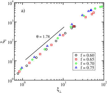
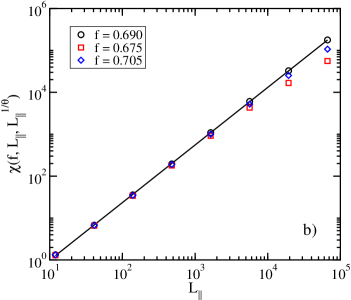
Figure 1: a) Correlation lengths in the q-model, computed at fixed $L_{\parallel}=16384$ and variable $L_{\perp}\ll L_{\parallel}$, for different values of the threshold force $f$. b) Susceptibility $\chi(f,L_{\parallel},L_{\parallel}^{1/\theta})$ of the q-model for different values of $f$. The straight line corresponds to the best power-law fit, corresponding to $f=0.690$ and yielding a slope $\gamma/\nu_{\parallel}\simeq 1.37$.

In Fig. 1(a), we present the results of simulations of the q-model with fixed $L_{\parallel}=16384$ and $L_{\perp}$ running from $16$ up to $2048$, for different values of $f$. Correlation lengths were computed as is customarily done in anisotropic systems [26]: For each cluster $c$ of connected forces that is composed by a set of vertices $\{x_{\parallel}^{(i)},x_{\perp}^{(i)}\}$, with $i=1,\ldots,s$, we define the quantities

$$R_{\parallel}(c)=\frac{1}{s}\sum_{i=1}^{s}|x_{\parallel}^{m}-x_{\parallel}^{(i)}|,\qquad R_{\perp}^{2}(c)=\frac{1}{s}\sum_{i=1}^{s}(x_{\perp}^{m}-x_{\perp}^{(i)})^{2},$$ (17)

where $x_{\parallel}^{m}$ and $x_{\perp}^{m}$ are the coordinates of some reference point within the cluster. We have chosen the point with the highest longitudinal coordinate and the average $x_{\perp}$ coordinate, respectively. Then, the correlation lengths are defined as

$$\xi_{\parallel}=\frac{\sum_{s}^{\prime}R_{\parallel}(s)s^{2}n(s,f)}{\sum_{s}^{\prime}s^{2}n(s,f)},\qquad\xi_{\perp}^{2}=\frac{\sum_{s}^{\prime}R_{\perp}^{2}(s)s^{2}n(s,f)}{\sum_{s}^{\prime}s^{2}n(s,f)},$$ (18)

where the prime indicates that one has to exclude the spanning clusters from the sum over cluster sizes. From the plots in Fig. 1(a), in which we have represented the data providing a best power-law fitting, we conclude that the percolation threshold is located in the vicinity of $f\sim 0.70$. Moreover, a linear regression for the smallest values of $\xi_{\perp}$ yields an estimate of the anisotropy exponent $\theta=1.78\pm 0.05$.

Once the exponent $\theta$ has been estimated, we can proceed with the full FSS analysis. In the first place, we focus on the behavior of the susceptibility $\chi(f,L_{\parallel},L_{\parallel}^{1/\theta})$ computed for $L_{\parallel}$ ranging from $12$ to $66451$. In Fig. 1(b) we represent the susceptibility as a function of $L_{\parallel}$ for different values of $f$. As can be seen in the plot, the best power law behavior for $\chi(f,L_{\parallel},L_{\parallel}^{1/\theta})$ is obtained for the threshold force $f_{c}=0.690\pm 0.005$; significant deviations can be observed for slightly larger and smaller values of $f$. A linear regression of $\chi(f,L_{\parallel},L_{\parallel}^{1/\theta})$ at the percolation threshold yields the exponent ratio $\gamma/\nu_{\parallel}=1.37\pm 0.01$.

The numerical analysis of the full normalized cluster size distribution at the percolation threshold can be performed using the moment analysis technique developed for the study of self-organized critical systems [27]. The $k$-th moment $M_{k}$ of the cluster distribution is defined as

$$M_{k}=\sum_{s}s^{k}n(s,f_{c},L_{\parallel},L_{\parallel}^{1/\theta})),$$ (19)

At the percolation threshold, when the cluster number is given by Eq. (13), we have that $M_{k}(L_{\parallel})\sim L_{\parallel}^{\alpha(k)}$, where the $k$-dependent exponent is given by

$$\alpha(k)=D_{\parallel}k+D_{\parallel}(1-\tau).$$ (20)

Thus, computing $M_{k}(L_{\parallel})$ as a function of $L_{\parallel}$ for different system sizes provides information on $\alpha(k)$, which should be a linear function of $k$ of the form $\alpha(k)=\alpha_{0}+k\alpha_{1}$, from which we obtain $D_{\parallel}=\alpha_{1}$ and $\tau=1-\alpha_{0}/\alpha_{1}$. The correctedness of exponent’s values can be checked by means of a data collapse technique: Noticing that the normalized cluster number $n(s,f_{c})$ scales as given by Eq.(13), then $L_{\parallel}^{\tau D_{\parallel}}n(s,f_{c})$ should collapse onto a universal function when plotted as a function of the rescaled variable $sL_{\parallel}^{-D_{\parallel}}$.

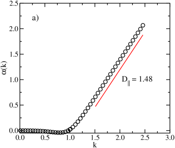
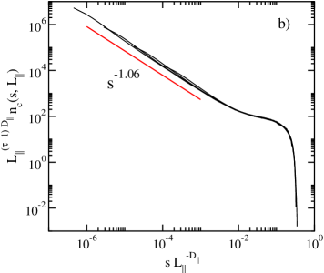
Figure 2: a) Plot of the $\alpha(k)$ functions for the q-model at the percolation threshold. The straight line is a least-squares fitting yielding the corresponding $D_{\parallel}$. b) Data collapse analysis of the integrated cluster number for the q-model at the percolation threshold. Systems sizes are $L_{\parallel}=478$, $1641$, $5634$, and $19349$.

In Fig. 2(a) we plot the $\alpha(k)$ evaluated from linear regressions of the moments $M_{k}(L_{\parallel})$, computed from numerical simulations at the percolation threshold with system sizes $L_{\parallel}=139$, $478$, $1641$, $5634$, and $19349$. A linear regression of this function, provides the values $D_{\parallel}=\alpha_{1}=1.48\pm 0.01$, and $\alpha_{0}=-1.57\pm 0.01$, from which we obtain $\tau=2.06\pm 0.02$. This last value can be checked against the scaling relation Eq. (6) (properly redefined for anisotropic systems), which leads to $\tau=3-\gamma/(D_{\parallel}\nu_{\parallel})\simeq 2.07$, in perfect agreement with the estimate from the regression of the $\alpha(k)$ function. In order to check the accuracy of these exponents for the q-model we perform a data collapse analysis of the integrated cluster number at the percolation threshold, defined as

$$n_{c}(s,L_{\parallel})=\sum_{s^{\prime}=s}^{\infty}n(s,L_{\parallel}).$$ (21)

In Fig.2(b) we observe that, as expected, the plots of the integrated cluster number, under the rescaling $s\to sL_{\parallel}^{-D_{\parallel}}$ and $n_{c}(s,L_{\parallel})\to L_{\parallel}^{(\tau-1)D_{\parallel}}n_{c}(s,L_{\parallel})$, collapse onto a single universal function for different values of $L_{\parallel}$.

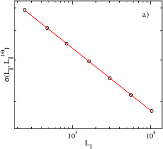
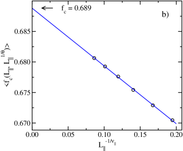
Figure 3: a) Fluctuations of the percolation threshold estimated by means of the bisection method. b) Extrapolation of the critical point from the bisection method.

We turn now our attention to the application of the bisection method. Fig. 3(a) shows the fluctuations $\sigma(L_{\parallel},L_{\parallel}^{1/\theta})$ computed as a function of $L_{\parallel}$. A linear regression provides the slope $1/\nu_{\parallel}$, from which we estimate the corresponding critical exponent $\nu_{\parallel}=3.77\pm 0.01$. With this result, we can compute the exponent $\gamma$ from the ratio $\gamma/\nu_{\parallel}$, obtaining $\gamma=5.18\pm 0.04$, and from Eq. (10), $\nu_{\perp}=2.12\pm 0.01$. Finally, using the previously computed exponent, we can plot $\langle f_{c}(L_{\parallel},L_{\parallel}^{1/\theta})\rangle$ as a function of $L_{\parallel}^{-1/\nu_{\parallel}}$, as in Fig. 3(b), which shows a good linear behavior, with an intercept with the vertical axis providing the value $f_{c}\simeq 0.689$ in excellent agreement with the threshold obtained from the analysis of the susceptibility.

5 Summary and discussion

In Table 1 we summarize the results we have obtained in our percolation analysis of the contact force network in the anisotropic q-model, compared with the exponents for isotropic and directed percolation, and with the exponents (or exponent ratios) available for the percolation transition in isotropic contact force networks [12, 13].

Table 1: Critical exponents for the percolation transition in the contact force network of q-model, compared with the values corresponding to isotropic percolation (IP) in two dimensions, directed percolation (DP) percolation in 1+1 dimensions, and the percolation transition in isotropic contact force networks (ICFN). Exponents from Refs. [15, 28, 12].

Exponent	q-model	IP	DP	ICFN
$\gamma$	$5.18\pm 0.04$	$43/18=2.3889$	$0.54386$	$2.8\pm 0.2$
$\nu_{\parallel}$	$3.77\pm 0.01$	$4/3=1.3333$	$1.73383$	$1.6\pm 0.1$
$\nu_{\perp}$	$2.12\pm 0.01$	$4/3=1.3333$	$1.09684$	$1.6\pm 0.1$
$D_{\parallel}$	$1.48\pm 0.01$	$91/48=1.8958$	$1.4727$	—
$\tau$	$2.06\pm 0.02$	$187/91=2.0549$	$2.108$	—
$\gamma/\nu_{\parallel}$	$1.37\pm 0.01$	$43/24=1.7917$	$0.3137$	$1.78\pm 0.02$

We note that the results obtained here for the q-model are compatible with those reported in Refs.[12, 13], namely $f_{c}\simeq 0.70$, $\gamma/\nu\simeq 1.38$, and $\nu\simeq 3.1$. Our method for estimating exponents is however more accurate and systematic, being at the same time capable of providing new exponents, not considered previously. This is specially evident for the exponent $\nu=3.1\pm 0.1$ quoted in [12], which is not discerning between the parallel and perpendicular directions.

The main conclusion extracted from the analysis of these exponents is that, at least in two dimensions, the percolation transition in the contact force network of anisotropic granular matter belongs to a universality class different from either anisotropic contact force networks and isotropic percolation. It is noteworthy that the change of universality goes thus beyond the simple presence of a preferred direction, as we can see from the comparison of the q-model exponents with those of directed percolation. Even though some exponents are similar, such as $\tau$ or $D_{\parallel}$, others are clearly different, out of the estimated error bars. The ultimate reason for this difference can be traced out in the presence of force correlations or arches [20]. The strength of these arches is enhanced in anisotropic models with a preferred direction for the propagation of weight, and explain the change in universality between different packing models. The origin of correlations is easy to understand in the present case: As we have defined it, the total force between rows is constant, imposing a global conservation law, superimposed to the local conservation of weights built in the definition of the model, Eq. (1). Global conservation prevents dissipation of stresses, and as a consequence any local build up of forces will propagate downwards unchecked and lead to the creation of arches in which strong forces are preferably connected to one another.

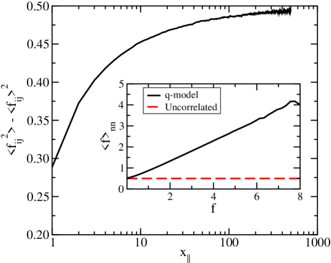
Figure 4: Standard deviation of the force distribution as a function of the longitudinal coordinate $x_{\parallel}$ article forces for two values of the longitudinal direction $x_{\parallel}$ in the massless q-model of size $500\times 500$, averaged over $500$ system realizations. Pressure per particle $P=1$.. Inset: Average nearest neighbor forces as a function of the force $f$.

The strong anisotropy and correlations in the force network of the q-model are checked in Fig. 4, where we plot the variance of the force distribution, computed at different heights $x_{\parallel}$, and which shows a marked dependence on this variable. In the case forces were uncorrelated at different $x_{\parallel}$ levels, and considering that forces are exponentially distributed [12], the variance should take the form $P^{2}/4=0.25$, clearly smaller than the numerically computed values. On the other hand, correlations between nearest neighbors are checked in the inset of Fig. 4, where we plot the average value $\langle f\rangle_{nn}$ of the forces connected to a given bond of force $f$ [29]. As we can see, this average value grows almost linearly with $f$, while in absence of correlations it should be equal to the average force $\langle f_{ij}\rangle=P/2=0.5$.

We conclude therefore that force networks in granular matter define different universality classes, depending on the symmetries imposed on the systems, universality classes that bear no resemblance with the corresponding ones in standard percolation, and are strongly affected by the strength of correlations in the overall force network structure. This result calls for further research in order to clarify the situation in more realistic settings, where the anisotropy might not be as strong as in the simple q-model [18].

References

- [1] Liu C and Nagel S (eds) 2001 Jamming and Rheology (London: Taylor and Francis)
- [2] Miguel M C and Rubí J M (eds) 2006 Jamming, Yielding and Irreversible Deformation in Condensed Matter (Lecture Notes in Physics vol 688) (Berlin: Springer Verlag)
- [3] Jaeger H M, Nagel S R and Behringer R P 1996 Rev. Mod. Phys. 68 1259
- [4] Dantu P 1967 Ann. Ponts Chaussees 4 144
- [5] Drescher A and de Josselin de Jong G 1972 J. Mech. Phys. Solids 20 337
- [6] Marone C 1998 Nature 391 69
- [7] Liu C H and Nagel S R 1992 Phys. Rev. Lett 68 2301
- [8] VandeWalle N, Lenaerts C and Dorbolo S 2001 Europhys. Lett. 53 197
- [9] Corwin E I, Jaeger H M and Nagel S R 2005 Nature 435 1075
- [10] Majmudar T S and Behringer R P 2005 Nature 435 1079
- [11] Newman M E J 2010 Networks: An introduction (Oxford: Oxford University Press)
- [12] Ostojic S, Somfai E and Nienhuis B 2006 Nature 439 828–830
- [13] Ostojic S and Nienhuis B 2007 Traffic and Granular Flow’05 ed Schadschneider A, Pöschel T, Kühne R, Schreckenberg M and Wolf D E (Berlin: Springer Verlag) pp 31–40
- [14] Bunde A and Havlin S 1991 Fractals and Disordered Systems ed Bunde A and Havlin S (Heidelberg: Springer Verlag) pp 51–95
- [15] Stauffer D and Aharony A 1994 Introduction to Percolation Theory 2nd ed (London: Taylor & Francis)
- [16] Privman V 1990 Finite Size Scaling and Numerical Simulation of Statistical Systems (Singapore: World Scientific)
- [17] Kinzel W 1983 Percolation Structures and Process (Annals of the Israel Physical Society vol 5) (Bristol: Adam Hilger) chap 18
- [18] Ostojic S, Vlugt T J H and Nienhuis B 2007 Phys. Rev. E 75 030301
- [19] Liu C H, Nagel S R, Schecter D A, Coppersmith S N, Majumdar S, Narayan O and Witten T A 1995 Science 269 513
- [20] Nicodemi M 1998 Phys. Rev. Lett. 80 1340
- [21] Stauffer D 1981 Disordered Systems and Localization (Lecture Notes in Physics vol 149) ed Castellani C, Di Castro C and Peliti L (Springer Berlin / Heidelberg) pp 9–25
- [22] Williams J K and Mackenzie N D 1984 J. Phys. A: Math. Gen. 17 3343–3351
- [23] Binder K and Wang J S 1989 J. Stat. Phys. 55 87–126
- [24] Redner S and Mueller P R 1982 Phys. Rev. B 26 5293–5295
- [25] Wang J S 1996 Journal of Statistical Physics 82 1409–1427
- [26] Pastor-Satorras R and Vespignani A 2000 Phys. Rev. E 62 6195
- [27] De Menech M, Stella A L and Tebaldi C 1998 Phys. Rev. E 58 R2677
- [28] Muñoz M A, Dickman R, Vespignani A and Zapperi S 1999 Phys. Rev. E 59 6175
- [29] Pastor-Satorras R, Vázquez A and Vespignani A 2001 Phys. Rev. Lett. 87 258701