Modeling of Low and High Frequency Noise by Slow and Fast Fluctuators

Abstract

We study the dynamics of dephasing in a quantum two-level system by modeling both $1/f$ and high-frequency noise by random telegraph processes. Our approach is based on a so-called spin-fluctuator model in which a noisy environment is modeled by a large number of fluctuators. In the continuous limit we obtain an effective random process (ERP) that is described by a distribution function of the fluctuators. In a simplified model, we reduce the ERP to the two (slow and fast) ensembles of fluctuators. Using this model, we study decoherence in a superconducting flux qubit and we compare our theoretical results with the available experimental data. We demonstrate good agreement of our theoretical predictions with the experiments. Our approach can be applied to many quantum systems, such as biological complexes, semiconductors, superconducting and spin qubits, where the effects of interaction with the environment are essential.

I Introduction

Decoherence is one of the main obstacles for building useful quantum devices. Understanding the mechanisms of decoherence and achieving long decoherence times is crucial for many fields of science and applications including quantum computation and quantum information nielsen , protein dynamics FFMP ; FC ; YF , dynamics of excitons and charge separation in biological complexes ECR ; SMR ; MSL ; CWW ; CBM , and the new and rapidly growing fields of NMR and MRI with ultra small (microtesla) magnetic fields EMV ; ZMV ; CHMM . In the latter case, the Larmor frequencies of the spin precession become relatively small (in the kHz region), causing the effects of $1/f$ noise become so important that noise suppression must be used.

In many situations the influence of noise can be modeled by an ensemble of two-level systems or fluctuators BGA ; GABS ; MSAM ; SSMM ; FAMP ; ICJM ; YBLA . Depending on the distribution of parameters of the fluctuators, such as amplitudes and switching rates, and coupling constants, this model can describe both Gaussian and non-Gaussian effects of noise BGA ; GABS ; MSAM . Recent experiments with Josephson qubits CSMM ; SLHN ; APNY , on the quantum dynamics of excitons in light-harvesting antennas in photosynthetic complexes ECR ; SMR ; MSL ; CWW ; CBM demonstrated these important contributions of noise and thermal fluctuations to decoherence, relaxation processes, and quantum coherence effects.

In this paper, we study relaxation and dephasing processes using a spin-fluctuator model BGA ; GABS . In the spin-fluctuator model, fluctuations are described by a random telegraph process (RTP) produced by $N$ fluctuators. Each fluctuator is characterized by two parameters: its amplitude and switching rate. Depending on the distribution function of fluctuators over amplitudes and switching rates, the RTP can describe noise for a broad range of frequencies using spectral characteristics that include both low- and high-frequencies noise.

We consider the noisy environment produced by a large number of fluctuators, $N\gg 1$. In the limit $N\rightarrow\infty$, we obtain an effective random process (ERP) described by a continuous distribution of fluctuators. We derive a closed system of integro-differential equations for functions averaged over the ERP. Even though this system of equations is closed, it is still very complicated for direct analysis and even for numerical solutions.

We study two approximations in which these equations are reduced to a system of differential equations. The first one we call the Gaussian approximation, because, as we demonstrate, in the simplest case of a two-level system (qubit) under the influence of an ERP, it yields the relation: $\langle\exp(i\varphi)\rangle=\exp(-{\langle\varphi^{2}/2\rangle})$, where $\varphi$ is the random angle of the Bloch vector. This Gaussian approximation is widely used in theoretical and experimental research to descre the influence of noise on quantum systems MSAM ; ICJM ; YHNN ; BMAH ; HJBJ ; KRDD ; MNAL . In many situations, this approximation is very useful because (i) it captures some important properties of noisy dynamics and (ii) it is simple to apply. However, the Gaussian approximation does not describe different “non-Gaussian” effects which can play a significant role.

Our second approximation is based on two effective fluctuators which include both low and high frequency noisy components. We show that this approximation goes beyond the Gaussian approach and better describes the experimental results for a superconducting flux qubit in a noisy environment YHNN .

Our main results

• We create a new model based on an effective random process (ERP) that includes both slow (low-frequencies) and fast (high-frequencies) fluctuators. This model can describe the influence of noise on a quantum system over a wide frequency range.

• For the functions averaged over the ERP, we obtain an integro-differential master equation which we reduce to a closed system of differential equations in two approximations: (i) a Gaussian approximation and (ii) an approximation of two-effective fluctuators. Both of these approximations describe, to some extent, the contributions from low and high frequency noise.

• We demonstrate that the two-effective fluctuator approximation accurately models “non-Gaussian” effects observed in experiments with superconducting flux qubits YHNN .

• We show that the two-effective-fluctuators model better describes the suppression of $1/f$ noise in experiments involving echo decay in superconducting flux qubits YHNN .

This paper is organized as follows. In Sec. II, a general model of noise based on ERP is introduced that describes both low-frequency ($1/f$) and high-frequency noise. In Sec. III, we use the reduced density matrix approach to describe the interaction of a quantum system with its environment by a master equation. For two cases (i) the Gaussian approximation and (ii) the two effective- fluctuator model, we reduce the system of integro-differential equations to a closed system of differential equations. In Sec. IV, the general method developed in Secs. II and III is applied to describe the decoherence of a superconducting flux qubit for free induction decay and for echo decay experiments. In the same Sec. IV, we compare our theoretical predictions with available experimental data and demonstrate a good agreement with experiments. We conclude in Sec. V with a discussion of our results. In the Appendices we present some technical details.

II Description of noise using a random telegraph process

To describe noise we use the spin-fluctuator model developed in BGA ; GABS . In this model, noise is described by a sum of $N$ uncorrelated fluctuators, $\xi_{N}=\sum^{N}_{i=1}\zeta_{i}(t)$, where $\zeta_{i}(t)$ is a random telegraph process (RTP). The variable, $\zeta_{i}(t)$, takes the values, $-a_{i}$ or $a_{i}$. Consequently, $\zeta^{2}_{i}(t)=a^{2}_{i}=\rm const$.

The RTP obeys following relations BGA ; KV1 ; KV2 ; KV3

$$\langle{\zeta}_{i}(t)\rangle=0,$$ (1)

$$\langle{\zeta}_{i}(t){\zeta}_{j}(t^{\prime})\rangle=\delta_{ij}a^{2}_{i}e^{-2\gamma_{i}|t-t^{\prime}|}.$$ (2)

The amplitude, $a_{i}$, together with the switching rate, $\gamma_{i}$, completely characterize the $i$-th fluctuator. The correlation function related to $\xi_{N}(t)$ is defined as, $\chi_{N}(|t-t^{\prime}|)=\langle\xi_{N}(t)\xi_{N}(t^{\prime})\rangle$. Using Eqs. (1) and (2), we obtain

$$\chi_{N}(|t-t^{\prime}|)=\sum^{N}_{i=1}a^{2}_{i}e^{-2\gamma_{i}|t-t^{\prime}|}.$$ (3)

Further, assuming $N\gg 1$, we consider continuous distributions of amplitudes and switching rates. The corresponding correlation function, $\chi(t)=\lim_{N\rightarrow\infty}\chi_{N}(t)$, can be written as

$$\chi(|t-t^{\prime}|)=\iint dw(\sigma,\gamma)\sigma^{2}e^{-2\gamma|t-t^{\prime}|},$$ (4)

where, $\sigma^{2}=\lim_{N\rightarrow\infty}Na^{2}$, and $dw(\sigma,\gamma)$ depends on the specific distributions of amplitudes and switching rates. The random process described by the function, $\xi(t)=\lim_{N\rightarrow\infty}\xi_{N}(t)$, we call an effective random process (ERP).

In order to model the characteristic behavior of the spectral density of noise in different frequency domains, we introduce a family of random variables and distributions, $\{\xi_{n}(t),dw_{n}(\sigma,\gamma)\}$. In particular, $n=1$ corresponds to low-frequency ($1/f$) noise, and $n=2$ corresponds to the Lorentzian spectrum for high frequencies. (See Appendix C for details.)

Accordingly, we introduce the ERP as $\xi(t)=\sum_{n}\xi_{n}(t)$, where each $\xi_{n}(t)$ is an independent source of noise. This implies $\langle\xi_{m}(t)\xi_{n}(t^{\prime})\rangle=0$ $(m\neq n)$. As shown in the Appendix A, the corresponding spectral density $S_{n}(\omega)$ behaves as $S_{n}(\omega)\sim 1/\omega^{n}$ in some region of frequencies. The total correlation function is a sum of the partial correlation functions, $\chi(|t-t^{\prime}|)=\sum_{n}\chi_{n}(|t-t^{\prime}|)$, where

$$\chi_{n}(|t-t^{\prime}|)=\iint dw_{n}(\sigma,\gamma)\sigma^{2}e^{-2\gamma|t-t^{\prime}|}.$$ (5)

In this paper, we adopt the simple model introduced in BGA for uncorrelated $\sigma$ and $\gamma$. We define the distribution function as

$$dw_{n}(\sigma,\gamma)=\delta(\sigma-\sigma_{n}){\mathcal{P}}_{n}(\gamma)d\sigma d\gamma,$$ (6)

where $\sigma_{n}$ is a typical value of the amplitude and

$${\mathcal{P}}_{n}(\gamma)d\gamma=A_{n}\Theta(\gamma_{c_{n}}-\gamma)\Theta(\gamma-\gamma_{m_{n}})\displaystyle\frac{d\gamma}{\gamma^{n}}.$$ (7)

Here, $\Theta(x)$, is a step-function; and $\gamma_{m_{n}}$ and $\gamma_{c_{n}}$ are the lower and upper switching rates, respectively. The normalization constant, $A_{n}$, is:

$$A_{n}=\left\{\begin{array}[]{ll}\displaystyle\frac{1}{\ln(\gamma_{c_{1}}/\gamma_{m_{1}})},&n=1\\ &\\ \displaystyle\frac{(n-1)\gamma^{n-1}_{m_{n}}}{(1-\gamma^{n-1}_{m_{n}}/\gamma^{n-1}_{c_{n}})},&n\neq 1\end{array}\right.$$ (11)

In the following, we restrict ourselves to two important cases: $n=1$ and $n=2$, which are related to $1/f$ noise and to high-frequency noise with the corresponding spectral densities. (The case for arbitrary $n$ is analyzed in Appendix C.) We denote $\gamma_{m}=\gamma_{m_{1}}$, $\gamma_{c}=\gamma_{c_{1}}$, and $\gamma_{0}=\gamma_{c_{2}}$. For the distribution functions, ${\mathcal{P}}_{1}(\gamma)$ and ${\mathcal{P}}_{2}(\gamma)$, we impose conditions at the point $\gamma=\gamma_{c}$, so that $\gamma_{m_{2}}=\gamma_{c_{1}}=\gamma_{c}$ $(\gamma_{m}<\gamma_{c}<\gamma_{0})$.

Using Eq. (167) (Appendix C), we obtain,

$$\chi_{1}(\tau)=\sigma^{2}_{1}A_{1}(E_{1}(2\gamma_{m}\tau)-E_{1}(2\gamma_{c}\tau)),$$ (12)

$$\chi_{2}(\tau)=\sigma^{2}_{2}A_{2}\bigg{(}\frac{E_{2}(2\gamma_{c}\tau)}{\gamma_{c}}-\frac{E_{2}(2\gamma_{0}\tau)}{\gamma_{0}}\bigg{)}.$$ (13)

Computation of the spectral density,

$$S_{n}(\omega)=\frac{1}{\pi}\int\limits_{0}^{\infty}\chi_{n}(\tau)\cos(\omega\tau)d\tau,$$ (14)

yields

$$S_{1}(\omega)=\frac{\sigma^{2}_{1}A_{1}}{\pi\omega}\bigg{(}\arctan\Big{(}\frac{\omega}{2\gamma_{m}}\Big{)}-\arctan\Big{(}\frac{\omega}{2\gamma_{c}}\Big{)}\bigg{)},$$ (15)

$$S_{2}(\omega)=\frac{\sigma^{2}_{2}A_{2}}{\pi\omega^{2}}\ln\bigg{(}\frac{1+\omega^{2}/4\gamma_{c}^{2}}{1+\omega^{2}/4\gamma_{0}^{2}}\bigg{)},$$ (16)

where $A_{1}=1/\ln(\gamma_{c}/\gamma_{m})$ and $A_{2}=\gamma_{c}/(1-\gamma_{c}/\gamma_{0})$.

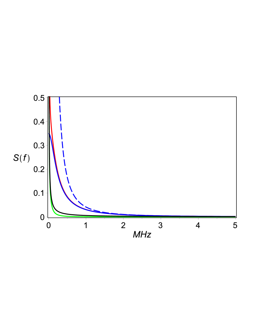
Figure 1: Spectral density of noise ($2\gamma_{m}=1\,\rm s^{-1}$, $2\gamma_{c}=1\,\rm\mu s^{-1}$, $2\gamma_{0}=10\,\rm\mu s^{-1}$, $\sigma_{1}=\sigma_{2}=1$, $\omega=2\pi f$). Red line: The total spectral density, $S(f)=S_{1}(f)+S_{2}(f)$. Green line: Contribution of the slow fluctuators described by $S_{1}(f)$. Blue line: Contribution of the fast fluctuators described by $S_{2}(f)$. Blue dashed line: The Lorentzian spectrum, $S_{L}(f)\sim 1/f^{2}$. Black line: The spectral density of $1/f$ noise, $S_{1/f}(f)=A/(2\pi f)$.

From Eqs. (15) and (16) it follows that, in the interval, $\gamma_{m}<\omega<\gamma_{c}$, the spectral density $S_{1}(\omega)$ describes $1/f$ noise. Indeed, in this interval $S_{1}(\omega)\approx A/\omega$, where $A=\sigma^{2}_{1}/(2\ln(\gamma_{c}/\gamma_{m}))$, and $\gamma_{m}$ and $\gamma_{c}$ are related to the infrared, $\omega_{m}=2\gamma_{m}$, and the ultraviolet, $\omega_{c}=2\gamma_{c}$, frequency cutoffs, respectively (Appendix C). For $S_{2}(\omega)$, we obtain the following asymptotic behavior: $S_{2}(\omega)\sim 1/\omega^{2}$ ($\omega\gg\omega_{c}$). Thus, asymptotically $S_{2}(\omega)$ has a Lorentzian spectrum.

To estimate the relative contributions of different processes for low- and high-frequency noise, we evaluate the relation, $S_{2}(\omega)/S_{1}(\omega)$ at frequencies $\omega\approx 0$ and $\omega\approx\omega_{c}$. A simple computation yields the following rough estimate:

$$\frac{S_{2}(\omega)}{S_{1}(\omega)}\sim\left\{\begin{array}[]{ll}\displaystyle\frac{\sigma^{2}_{2}}{\sigma^{2}_{1}}\frac{\gamma_{m}\ln(\gamma_{c}/\gamma_{m})}{\gamma_{c}},&\omega\approx 0,\\ \\ \displaystyle\frac{\sigma^{2}_{2}}{\sigma^{2}_{1}}\ln(\gamma_{c}/\gamma_{m}),&\omega\approx\omega_{c}.\end{array}\right.$$ (20)

Taking values typical for superconducting qubits, $2\gamma_{m}\approx 1\,\rm s^{-1}$ and $2\gamma_{c}\approx 1\,{\rm\mu s}^{-1}$, we obtain

$$\frac{S_{2}(\omega)}{S_{1}(\omega)}\sim\left\{\begin{array}[]{ll}\displaystyle 10^{-5}{\sigma^{2}_{2}}/{\sigma^{2}_{1}},&\omega\approx 0,\\ \\ \displaystyle 10\,{\sigma^{2}_{2}}/{\sigma^{2}_{1}},&\omega\approx\omega_{c}.\end{array}\right.$$ (24)

Thus, for low-frequency noise the main contribution near $\omega=0$ is provided by slow fluctuators (SF) with the switching rates, $\gamma$, being in the interval $(\gamma_{m},\gamma_{c})$. However, for high frequencies, $\omega\gtrsim\omega_{c}$, the contribution of fast fluctuators (FF) with $\gamma\gtrsim\gamma_{c}$ dominates. (See Fig. 1.)

III Master equation for averaged density matrix

We consider a quantum system governed by the Hamiltonian, ${\mathcal{H}(t)}$ (generally time-dependent), depending on control parameters, $\lambda_{i}$ ( external flux, biased current, critical current, etc). The noise associated with fluctuations of these parameters is described by random functions, $\delta\lambda_{i}(t)$. For simplicity, we restrict ourselves to only one fluctuating parameter, $\delta\lambda(t)$, denoting it as $\xi(t)$. Generalization for many parameters is straightforward. Expanding the Hamiltonian to first order in $\xi(t)$, we obtain

$${\mathcal{H}(t)}={\mathcal{H}}_{0}(t)+{\mathcal{V}}(t)\xi(t).$$ (25)

To include the effects of a thermal bath, we use the reduced density matrix approach leading to the master equation:

$$\frac{d\rho}{dt}=-i[{\mathcal{H}(t)},\rho]+{\mathcal{L}}\rho,$$ (26)

where the superoperator, ${\mathcal{L}}$, describes coupling to the bath.

Using (25), one can recast Eq. (26) as

$$\frac{d\rho(t)}{dt}=-i[{\mathcal{H}}_{0}(t),\rho(t)]+{\mathcal{L}}\rho(t)$$

$$-i[\xi(t){\mathcal{V}}(t),\rho(t)].$$ (27)

For the average density matrix, this yields

$$\frac{d\langle\rho(t)\rangle}{dt}=-i[{\mathcal{H}}_{0}(t),\langle\rho(t)\rangle]+{\mathcal{L}}\langle\rho(t)\rangle$$

$$-i[{{\mathcal{V}}}(t),\langle X(t)\rangle],$$ (28)

where $\langle X(t)\rangle=\langle{\xi}(t)\rho(t)\rangle$, and the average $\langle{\;}\rangle$ is taken over the random process describing the noise.

As before, we assume that fluctuations are produced by the ERP, so that $\xi(t)=\sum_{n}\xi_{n}(t)$, and the correlation function can be written as a sum of the partial correlation functions, $\chi(|t-t^{\prime}|)=\sum_{n}\chi_{n}(|t-t^{\prime}|)$. (See Eq. 5.)

Eq. (III), an integro-differential equation, is rather complicated. However, in two important cases (the Gaussian approximation and the approximation by effective fluctuators) we obtain a closed system of first order differential equations (Appendix B). Below we summarize our results for $\xi(t)=\xi_{1}(t)+\xi_{2}(t)$, where $\xi_{1}(t)$ is related to slow fluctuators leading to $1/f$ noise, and $\xi_{2}(t)$ is related to fast fluctuators leading to high-frequency noise.

The Gaussian approximation. Applying the method described in Appendix B, we find that, in the Gaussian approximation, the master equation can be recast as follows

$$\frac{d\langle\rho(t)\rangle}{dt}= -i[{\mathcal{H}}_{0}(t),\langle\rho(t)\rangle]+{\mathcal{L}}\langle\rho(t)\rangle$$

$$-[{\mathcal{V}}(t),[{\mathcal{K}}(t),\langle\rho(t)\rangle]]+{\mathcal{O}}(\parallel{\mathcal{V}}\parallel^{4}),$$ (29)

where ${\mathcal{K}}(t)=\int_{0}^{t}dt^{\prime}\chi(t-t^{\prime})U^{\dagger}(t)\tilde{\mathcal{V}}(t^{\prime})U(t)$. We denote $\tilde{\mathcal{V}}(t)=U(t){\mathcal{V}}(t)U^{\dagger}(t)$, and

$$U(t)=T\Big{(}e^{i\int\limits_{0}^{t}{\mathcal{H}}_{0}(t^{\prime})dt^{\prime}}\Big{)}.$$ (30)

The approximation by two effective fluctuators. In the approximation by two effective fluctuators, the set of slow, $\xi_{1}(t)$, and fast, $\xi_{2}(t)$, fluctuators is approximated by two effective fluctuators: one for SF and the other for FF. The total correlation function, $\chi(|t-t^{\prime}|)=\chi_{1}(|t-t^{\prime}|)+\chi_{2}(|t-t^{\prime}|)$ , is approximated as

$$\chi_{n}(|t-t^{\prime}|)\approx{a^{\ast}_{n}}^{2}e^{-2\gamma^{\ast}_{n}|t-t^{\prime}|},\quad n=1,2,$$ (31)

where $a_{n}^{\ast}$ and $\gamma^{\ast}_{n}$ (the effective amplitude and switching rate) are defined as follows: ${a^{\ast}_{n}}^{2}=\chi_{n}(0)$ and $\gamma^{\ast}_{n}=-(1/2)d\ln\chi(t)/dt|_{t=0}$. (For details, see Appendix B.)

Applying the method developed in Appendix B for an arbitrary system of stochastic first-order ordinary differential equations, we obtain from Eq. (III) the following closed system of ordinary differential equations:

$$\frac{d}{dt}{\langle\rho(t)\rangle} = -i[{\mathcal{H}}_{0}(t),{\langle\rho\rangle}]+{\mathcal{L}}{\langle\rho\rangle}-i[{\mathcal{V}}(t),\langle X_{1}(t)\rangle]-i[{\mathcal{V}}(t),\langle X_{2}(t)\rangle],$$ (32)

$$\frac{d}{dt}{\langle X_{1}(t)\rangle} = -2\gamma^{\ast}_{1}\,{\langle X_{1}(t)\rangle}-i[{\mathcal{H}}_{0}(t),{\langle X_{1}(t)\rangle}]+{\mathcal{L}}{\langle X_{1}(t)\rangle}$$ (33)

$$-i{a_{1}^{\ast}}^{2}[{{\mathcal{V}}}(t),\langle\rho(t)\rangle]-i[{{\mathcal{V}}}(t),\langle X_{12}(t)\rangle],$$

$$\frac{d}{dt}{\langle X_{2}(t)\rangle} = -2\gamma^{\ast}_{2}\,{\langle X_{2}(t)\rangle}-i[{\mathcal{H}}_{0}(t),{\langle X_{1}(t)\rangle}]+{\mathcal{L}}{\langle X_{2}(t)\rangle}$$ (34)

$$-i{a_{2}^{\ast}}^{2}[{{\mathcal{V}}}(t),\langle\rho(t)\rangle]-i[{{\mathcal{V}}}(t),\langle X_{12}(t)\rangle],$$

$$\frac{d}{dt}{\langle X_{12}(t)\rangle} = -2(\gamma^{\ast}_{1}+\gamma^{\ast}_{2}){\langle X_{12}(t)\rangle}-i[{\mathcal{H}}_{0}(t),{\langle X_{12}(t)\rangle}]+{\mathcal{L}}{\langle X_{12}(t)\rangle}$$ (35)

$$-i{a_{1}^{\ast}}^{2}[{{\mathcal{V}}}(t),\langle X_{2}(t)\rangle-i{a_{2}^{\ast}}^{2}[{{\mathcal{V}}}(t),\langle X_{1}(t)\rangle],$$

where $\langle{X}_{1}(t)\rangle=\langle\xi_{1}(t){\rho}(t)\rangle$, $\langle{X}_{2}(t)\rangle=\langle\xi_{2}(t){\rho}(t)\rangle$ and $\langle{X}_{12}(t)\rangle=\langle\xi_{1}(t)\xi_{2}(t){\rho}(t)\rangle$.

IV Non-Gaussian noise and decoherence in a superconducting phase qubit

In this section, the general method developed in Secs. 2 and 3 is applied to describe relaxation effects in a superconducting qubit. The effective Hamiltonian for a superconducting qubit can be written as YHNN (see also references therein),

$${\mathcal{H}}(t)=-\frac{1}{2}{\boldsymbol{\Omega(t)}}\cdot\boldsymbol{\sigma},$$ (36)

where $\boldsymbol{\sigma}$ denotes the Pauli matrices. We assume that ${\mathcal{H}(t)}$ depends on the control parameters, $\lambda_{i}$, of the system, including external flux, biased current, critical current, etc. Limiting ourselves to a single fluctuating parameter, $\lambda$, and expanding the Hamiltonian in Eq. (36) to first order in the fluctuations, $\delta\lambda(t)$, we obtain,

$${\mathcal{H}}(t)=-\frac{1}{2}{\boldsymbol{\Omega}}\cdot\boldsymbol{\sigma}-\frac{1}{2}\delta\lambda(t)\frac{\partial\boldsymbol{\Omega}}{\partial\lambda}\cdot\boldsymbol{\sigma},$$ (37)

where, for simplicity, we assume that ${\boldsymbol{\Omega}}$ does not depend on $t$. In the eigenbasis of the unperturbed Hamiltonian, Eq. (29) takes the form

$${\mathcal{H}}(t)= -\frac{1}{2}\Omega\sigma_{z}-\frac{1}{2}D_{\lambda,z}\delta\lambda(t)\sigma_{z}$$

$$-\frac{1}{2}D_{\lambda,\bot}\delta\lambda(t)\sigma_{\bot},$$ (38)

where $D_{\lambda,z}=\partial\Omega/\partial\lambda$ and $\sigma_{\bot}$ denotes the transverse spin components, either $\sigma_{x}$ or $\sigma_{y}$. (We adopt the notation of Ref. ICJM .)

Below, in the framework of the ERP model, we obtain the relaxation rates, and compare our results with the results which follow from the well-known Bloch-Redfield (BR) theory BF1 ; Rag applied to the external noise ICJM . Before proceeding, we present here some important results of the BR approach.

In BR theory, the dynamics of a two-level system is described by two rates: the longitudinal relaxation rate, $\Gamma_{1}=T_{1}^{-1}$, and the transverse relaxation rate, $\Gamma_{2}=T_{2}^{-1}$. BR theory is valid if $T_{1},T_{2}\gg\tau_{c}$, where $\tau_{c}$ is the fluctuation correlation time. The transverse relaxation rate, $\Gamma_{2}$, is a combination of $\Gamma_{1}$ and the so-called “pure dephasing” rate, $\Gamma_{\varphi}$,

$$\Gamma_{2}=\frac{1}{2}\Gamma_{1}+\Gamma_{\varphi}.$$ (39)

In terms of the spectral density of noise, $S_{\lambda}(\omega)$, these rates are defined as follows ICJM :

$$\Gamma_{1}=\pi D^{2}_{\lambda,\bot}S_{\lambda}(\Omega),$$ (40)

$$\Gamma_{\varphi}=\pi D^{2}_{\lambda,z}S_{\lambda}(0).$$ (41)

In our approach, fluctuations of the parameter, $\lambda$, are described by an ERP. Thus, $\delta\lambda(t)=\sum_{n}\xi_{n}(t)$. Further, we restrict ourselves to consideration only the case, $n=1,2$. Then, $\delta\lambda(t)=\xi_{1}(t)+\xi_{2}(t)$, where $\xi_{1}(t)$ describes the contribution to the ERP of SF, and $\xi_{2}(t)$ describes the contribution of FF. The spectral density of noise can be written as $S_{\lambda}(\omega)=S_{1}(\omega)+S_{2}(\omega)$.

Since only FFs have small correlation times and satisfy the conditions of applicability of BR theory, we use the spectral density of FFs given by Eq. (16) to calculate the relaxation and dephasing rates provided by the BR theory. We obtain

$$\Gamma_{1}=\pi D^{2}_{\lambda,\bot}S_{2}(\Omega)=D^{2}_{\lambda,\bot}\frac{\sigma^{2}_{2}\gamma_{c}}{\Omega^{2}(1-{\gamma_{c}}/{\gamma_{0}})}\ln\bigg{(}\frac{1+\Omega^{2}/4\gamma_{c}^{2}}{1+\Omega^{2}/4\gamma_{0}^{2}}\bigg{)},$$ (42)

$$\Gamma_{\varphi}=\pi D^{2}_{\lambda,z}S_{2}(0)=D^{2}_{\lambda,z}\frac{\sigma^{2}_{2}}{4\gamma_{c}}\bigg{(}1+\frac{\gamma_{c}}{\gamma_{0}}\bigg{)}.$$ (43)

Note, that the validity of the BR theory is restricted by the condition: $\Gamma_{1}\tau_{2},\Gamma_{2}\tau_{2}\ll 1$, where $\tau_{2}=({1}/{2\gamma_{c}})(1+{\gamma_{c}}/{\gamma_{0}})$ is the effective correlation time of the FF.

The above effective rates can also be obtained directly from the averaged expressions for the partial rates,

$$\Gamma_{1}=D^{2}_{\lambda,\bot}\int\limits_{\gamma_{c}}^{\gamma_{0}}\frac{{\sigma}_{2}^{2}\gamma}{4\gamma^{2}+\Omega^{2}}\,dw_{2}(\gamma),$$ (44)

$$\Gamma_{\varphi}=D^{2}_{\lambda,z}\int\limits_{\gamma_{c}}^{\gamma_{0}}\frac{{\sigma}_{2}^{2}}{2\gamma}\,dw_{2}(\gamma).$$ (45)

IV.1 Pure decoherence

Let us consider the Hamiltonian (IV) for a pure decoherence case. Then $D_{\lambda,\bot}=0$, and the Hamiltonian ${\mathcal{H}}(t)$ takes the form

$${\mathcal{H}}(t)=-\frac{1}{2}\Omega(t)\sigma_{z}-\frac{1}{2}D_{\lambda,z}\delta\lambda(t)\sigma_{z},$$ (46)

where $D_{\lambda,z}=\partial\Omega/\partial\lambda$.

The equation of motion for the density matrix, $i\dot{\rho}=[\mathcal{H}(t),\rho]$, reduces to only one component:

$$\frac{d}{dt}{\rho}_{01}=i\Omega(t){\rho}_{01}+iD_{\lambda,z}\delta\lambda(t){\rho}_{01}.$$ (47)

The matrix elements, ${\rho}_{00}$ and ${\rho}_{11}$, are constant.

Setting ${\rho_{01}(t)}=\tilde{\rho}_{01}(t)e^{i\varphi_{0}(t)}$, where $\varphi_{0}(t)=\int^{t}_{0}\Omega dt$ is a regular phase, we find that $\tilde{\rho}_{01}(t)$ satisfies the following differential equation:

$$\frac{d}{dt}{\tilde{\rho}}_{01}(t)=iD_{\lambda,z}\delta\lambda(t)\tilde{\rho}_{01}(t).$$ (48)

Its solution can be written as

$${\tilde{\rho}}_{01}(t)=e^{i\varphi(t)}\rho_{01}(0),$$ (49)

where $\varphi(t)=\int\limits_{0}^{t}D_{\lambda,z}\delta\lambda(t)dt$ is a random phase. After averaging over the random process, we obtain $\langle{\tilde{\rho}}_{01}(t)\rangle=\langle e^{i\varphi(t)}\rangle\rho_{01}(0)$. This yields $\langle{\rho}_{01}(t)\rangle=e^{i\varphi_{0}(t)}\langle e^{i\varphi(t)}\rangle\rho_{01}(0)$. Thus, the problem of obtaining exact solution of Eq. (47) reduces to the computation of the generating functional, $\langle e^{i\varphi(t)}\rangle$.

Returning to Eq. (47), one can see that, for averaged components of the density matrix, it takes the form

$$\frac{d}{dt}\langle{\rho}_{01}(t)\rangle=i\Omega(t)\langle{\rho}_{01}(t)\rangle+iD_{\lambda,z}\langle\delta\lambda(t){\rho}_{01}(t)\rangle.$$ (50)

In what follows, we obtain solutions of Eq. (50) in the Gaussian approximation and in the two-effective-fluctuator approximation. We apply these solutions to describe two widely used experimental protocols: (i) free induction decay and (ii) echo decay. We compare our theoretical predictions with the experimental data YHNN , and demonstrate that the experimental results (i) are described by the Gaussian approximation and (ii) that the details of the dynamics of the signal decay can be understood by using slow and fast effective fluctuators. We also demonstrate that the approach based on two effective fluctuators allows one to fit the experimental data better.

IV.1.1 Gaussian approximation

In the Gaussian approximation Eq. (50) can be presented in the form

$$\frac{d}{dt}\langle{\rho}_{01}(t)\rangle=i\Omega(t)\langle{\rho}_{01}(t)\rangle$$

$$-D^{2}_{\lambda,z}\Big{(}\int\limits_{0}^{t}\chi(t-t^{\prime})dt^{\prime}\Big{)}\langle{\rho}_{01}(t)\rangle,$$ (51)

where $\chi(t-t^{\prime})=\langle\delta\lambda(t)\lambda(t^{\prime})\rangle$. Its solution can be written as

$$\langle{\rho}_{01}(t)\rangle=e^{i\varphi_{0}(t)}e^{-(1/2)\langle\varphi^{2}(t)\rangle}\langle{\rho}_{01}(0)\rangle,$$ (52)

where $\varphi_{0}(t)=\int_{0}^{t}\Omega(\tau)d\tau$ is a regular phase, $\varphi(t)=D_{\lambda,z}\int\limits_{0}^{t}\delta\lambda(t^{\prime})dt^{\prime}$ is the random phase accumulated during the time, $t$, and

$$\langle\varphi^{2}(t)\rangle=D^{2}_{\lambda,z}\int\limits_{0}^{t}\int\limits_{0}^{t}\chi(|t^{\prime}-t^{\prime\prime}|)dt^{\prime}dt^{\prime\prime},$$ (53)

is the variance of $\varphi(t)$.

Thus, in the Gaussian approximation, the random phase of the free-induction decay is Gaussian distributed, and we obtain the well-known result for the generating functional,

$$\langle e^{i\varphi(t)}\rangle=e^{-(1/2)\langle\varphi^{2}(t)\rangle}.$$ (54)

Using the spectral function of noise, $S_{\lambda}(\omega)$, one can rewrite (54) as BGA ; ICJM

$$\langle e^{i\varphi(t)}\rangle=\exp\Big{(}-\frac{t^{2}}{2}D^{2}_{\lambda,z}\int\limits_{-\infty}^{\infty}d\omega S_{\lambda}(\omega){\rm sinc}^{2}\frac{\omega t}{2}\Big{)},$$ (55)

where ${\rm sinc}\,x=\sin x/x$.

In the echo experiments, the total phase, $\psi(t)$, is defined as difference between two free evolutions, so that BGA ; ICJM

$$\psi(t)=D_{\lambda,z}\Bigg{(}\int\limits_{0}^{t/2}\delta\lambda(t^{\prime})dt^{\prime}-\int\limits_{t/2}^{t}\delta\lambda(t^{\prime})dt^{\prime}\Bigg{)}.$$ (56)

In the Gaussian approximation, we obtain

$$\langle e^{i\psi(t)}\rangle=e^{-(1/2)\langle\psi^{2}(t)\rangle},$$ (57)

where

$$\langle\psi^{2}(t)\rangle=D^{2}_{\lambda,z}\int\limits_{0}^{t}\int\limits_{0}^{t}dt^{\prime}dt^{\prime\prime}\chi(|t^{\prime}-t^{\prime\prime}|)$$

$$-4D^{2}_{\lambda,z}\int\limits_{0}^{t/2}dt^{\prime}\int\limits_{t/2}^{t}dt^{\prime\prime}\chi(|t^{\prime}-t^{\prime\prime}|).$$ (58)

In terms of the spectral density, the echo decay can be written as BGA ; ICJM

$$\langle e^{i\psi(t)}\rangle=\exp\Big{(}-\frac{t^{2}}{2}D^{2}_{\lambda,z}\int\limits_{-\infty}^{\infty}d\omega S_{\lambda}(\omega)\sin^{2}\frac{\omega t}{4}{\rm sinc}^{2}\frac{\omega t}{4}\Big{)}.$$ (59)

In Appendix C, we obtain explicit expressions for $\langle\varphi^{2}(t)\rangle$ and $\langle\psi^{2}(t)\rangle$.

Using the asymptotic formulae for the exponential integrals, $E_{n}(z)$, abr , we find that, for $\gamma_{m}t\ll 1$ ($\gamma_{c}t<1$), the free-induction decay produced by SF is given by

$$\langle e^{i\varphi(t)}\rangle=\exp\bigg{(}-{t^{2}}D^{2}_{\lambda,z}A\Big{(}\ln\frac{1}{2\gamma_{m}t}+{\mathcal{O}}(1)\Big{)}\bigg{)},$$ (60)

where $A=\sigma^{2}_{\xi_{1}}/(2\ln(\gamma_{c}/\gamma_{m}))$. Substituting $\omega_{m}=2\gamma_{m}$, we find that (60) is exactly the same expression that is used in the literature for estimating the quasistatic contribution of $1/f$ noise to the free-induction decay ICJM . In the same limit, for the echo decay we obtain

$$\langle e^{i\psi(t)}\rangle=\exp(-t^{2}D^{2}_{\lambda,z}A\ln 2),$$ (61)

which coincides with the corresponding formula obtained from Eq. (59) for $\omega_{m}t\ll 1$ CA .

The contribution of low frequencies, $\omega t\ll 1$, in (54) obtained in the limit $\gamma_{m}t,\gamma_{c}t\ll 1$, is

$$\langle e^{i\varphi(t)}\rangle=\exp\bigg{(}-\frac{t^{2}}{2}D^{2}_{\lambda,z}\sigma_{\xi_{1}}^{2}\bigg{)}.$$ (62)

This coincides with the corresponding expression widely used in the literature ICJM .

IV.1.2 Two-effective fluctuator model

In this Section, the SF and FF introduced above are approximately described by two effective fluctuators with the following correlation functions (see Appendix B),

$$\chi_{n}(|t-t^{\prime}|)\approx\sigma_{n}^{2}e^{-2\gamma_{n}|t-t^{\prime}|},\quad(n=1,2).$$ (63)

where

$$\gamma_{n}=-\frac{1}{2}\frac{\partial\ln(\chi_{n}(\tau))}{\partial\tau}\bigg{|}_{\tau=0},$$ (64)

the effective amplitude and switching rate being $\sigma_{n}$ and $\gamma_{n}$. Computation yields

$${\gamma}_{1}=\frac{\gamma_{c}-\gamma_{m}}{\ln(\gamma_{c}/\gamma_{m})},$$ (65)

$${\gamma}_{2}=\frac{\gamma_{c}\ln(\gamma_{0}/\gamma_{c})}{1-\gamma_{c}/\gamma_{0}}.$$ (66)

For the averaged functions: $\langle{\rho_{01}}(t)\rangle$, $\langle{X}_{1}(t)\rangle=\langle\xi_{1}(t){\rho_{01}}(t)\rangle$, $\langle{X}_{2}(t)\rangle=\langle\xi_{2}(t){\rho_{01}}(t)\rangle$ and $\langle{X}_{12}(t)\rangle=\langle\xi_{1}(t)\xi_{2}(t){\rho_{01}}(t)\rangle$, we obtain the following closed system of first-order differential equations:

$$\frac{d}{dt}\langle{\rho_{01}}(t)\rangle=i\Omega(t)\langle{\rho_{01}}(t)\rangle+iD_{\lambda,z}(\langle{X}_{1}(t)\rangle+\langle{X}_{2}(t)\rangle),$$ (67)

$$\frac{d}{dt}\langle{X}_{1}(t)\rangle=-2\gamma_{1}\langle{X}_{1}(t)\rangle+i\Omega(t)\langle{X}_{1}(t)\rangle+iD_{\lambda,z}(\langle{X}_{12}(t)\rangle+a^{2}_{1}\langle{\rho_{01}}(t)\rangle),$$ (68)

$$\frac{d}{dt}\langle{X}_{2}(t)\rangle=-2\gamma_{2}\langle{X}_{1}(t)\rangle+i\Omega(t)\langle{X}_{2}(t)\rangle+iD_{\lambda,z}(\langle{X}_{12}(t)\rangle+a^{2}_{2}\langle{\rho_{01}}(t)\rangle),$$ (69)

$$\frac{d}{dt}\langle{X}_{12}(t)\rangle=-2(\gamma_{1}+\gamma_{2})\langle{X}_{12}(t)\rangle+i\Omega(t)\langle{X}_{12}(t)\rangle+iD_{\lambda,z}(a^{2}_{2}\langle{X}_{1}(t)\rangle+a^{2}_{1}\langle{X}_{2}(t)\rangle).$$ (70)

The solution of Eqs. (67) - (70) can be written as,

$$\langle\rho_{01}(t)\rangle=e^{i\varphi_{0}(t)}\Phi_{1}(t)\Phi_{2}(t)\rho_{01}(0),$$ (71)

$$iD_{\lambda,z}\langle{X}_{1}(t)\rangle=e^{i\varphi_{0}(t)}{\dot{\Phi}}_{1}(t)\Phi_{2}(t)\rho_{01}(0),$$ (72)

$$iD_{\lambda,z}\langle{X}_{2}(t)\rangle=e^{i\varphi_{0}(t)}\Phi_{1}(t){\dot{\Phi}}_{2}(t)\rho_{01}(0),$$ (73)

$$D^{2}_{\lambda,z}\langle{X}_{12}(t)\rangle=-e^{i\varphi_{0}(t)}{\dot{\Phi}}_{1}(t){\dot{\Phi}}_{2}(t)\rho_{01}(0),$$ (74)

where $\varphi_{0}(t)=\int^{t}_{0}\Omega(t^{\prime})dt^{\prime}$. We denote by $\Phi_{i}(t)$ $(i=1,2)$ the generating functional of the RTP KV1 ; KV2 ; KV3 ,

$$\Phi_{i}(t)=\Big{\langle}\exp\Big{\{}i\int\limits_{0}^{t}d\tau\xi_{i}(\tau)v_{i}\Big{\}}\Big{\rangle},$$ (75)

where $v_{i}^{2}=D^{2}_{\lambda,z}a_{i}^{2}$. The generating functional satisfies the second order differential equation KV1 ; KV2 ; KV3 ,

$$\frac{d^{2}\Phi_{i}}{dt^{2}}+2\gamma_{i}\frac{d\Phi_{i}}{dt}+{v_{i}^{2}}\Phi_{i}=0,$$ (76)

with the initial conditions being $\Phi_{i}(0)=1$ and $d\Phi_{i}(0)/dt=0$.

Free induction and echo decay solutions for a single fluctuator. In the following, we consider solutions of Eq. (76) corresponding to free induction signal and echo signal experiments. Previously Eq. (76) was studied in BGA ; GABS1 ; GABS2 .

• The solution corresponding to the decay of the free induction signal is given by BGA ; PFFF ; GABS2

  $$\Phi^{f}_{i}(t)=\frac{e^{-\gamma_{i}t}}{\mu_{i}}\sinh({\gamma_{i}\mu_{i}t})$$

  $$+e^{-\gamma_{i}t}\cosh({\gamma_{i}\mu_{i}t}),$$ (77)

  where $\mu_{i}=\sqrt{1-{v_{i}}^{2}/\gamma_{i}^{2}}$.

• In the echo experiments, the $\pi$-pulse with duration, $\tau_{1}$, is applied at time, $\tau=t/2$, to switch the two states of qubit. It is assumed that $\tau_{1}\ll\tau$. The corresponding solution for the functional $\Phi^{e}_{i}(t)$, with the initial conditions $\Phi^{e}_{i}(0)=1$ and $d\Phi^{e}_{i}(0)/dt=0$, is written as BGA

  $$\Phi^{e}_{i}(t)= \frac{e^{-\gamma_{i}t}}{\mu_{i}^{2}}\big{(}\mu_{i}\sinh({\gamma_{i}\mu_{i}t})$$

  $$+\cosh({\gamma_{i}\mu_{i}t})+\mu_{i}^{2}-1\big{)}.$$ (78)

IV.2 Comparison with experiment

In this section, we compare our theoretical predictions with the experimental data obtained in YHNN and the theoretical results of the model ZJR . The measurement of the decoherence due to $1/f$ noise was done for the flux qubit described by the effective Hamiltonian YHNN ,

$$H_{0}=-\frac{\varepsilon}{2}\sigma_{z}-\frac{\Delta}{2}\sigma_{x},$$ (79)

with the energy difference between two eigenstates $E_{01}=\sqrt{\varepsilon^{2}+\Delta^{2}}$.

The diagonalized Hamiltonian, with the fluctuations only of $E_{01}$, can be written as

$$H=-\frac{E_{01}}{2}\sigma_{z}-\frac{1}{2}\sum_{a}D_{\lambda_{a},z}\delta\lambda_{a}(t)\,\sigma_{z},$$ (80)

where $D_{\lambda_{a},z}={\partial E_{01}}/{\partial\lambda_{a}}$, and the term, $\delta\lambda_{a}(t)$, describes the fluctuations of $\lambda_{a}$ in the Hamiltonian. In the experiments YHNN , the authors studied the decoherence due to fluctuations of (i) the normalized external flux, $n_{\phi}=\Phi_{\rm ex}/\Phi_{0}$, where $\Phi_{0}$ is the flux quantum, and (ii) the SQUID bias current, $I_{b}$. The contributions from different decoherence sources were separated, so that the fluctuations of $n_{\phi}$ and $I_{b}$ were observed independently.

We consider two approximations: (i) the two-effective fluctuator approximation and (ii) the Gaussian approximation.

IV.2.1 Two-effective-fluctuator approximation

In the approximation of two effective fluctuators, $\delta\lambda(t)=\xi_{1}(t)+\xi_{2}(t)$, and

$$\langle\xi_{i}(t)\xi_{j}(t^{\prime})\rangle=\delta_{ij}\sigma^{2}_{i}e^{-2\gamma_{i}t},\quad i=1,2.$$ (81)

Our task is to determine the fitting parameters: $(v_{1},\gamma_{1},v_{2},\gamma_{2}$), where $v_{i}^{2}=D^{2}_{\lambda,z}\sigma_{i}^{2}$, and

$${\gamma}_{1}=\frac{\gamma_{c}(1-\gamma_{m}/\gamma_{c})}{\ln(\gamma_{c}/\gamma_{m})},\quad{\gamma}_{2}=\frac{\gamma_{c}\ln(\gamma_{0}/\gamma_{c})}{1-\gamma_{c}/\gamma_{0}}.$$ (82)

The switching rates, $\gamma_{m}$ and $\gamma_{c}$, are chosen according to the available experimental data for the spectral behavior of $1/f$ noise, namely, $\gamma_{m}\sim 1\;\rm s^{-1}$ and $\gamma_{c}\sim 1\;\rm\mu s^{-1}$. Then, the only two free fitting parameters are $\gamma_{0}$ and $v_{2}$. Their values are chosen from the best fit of theoretical results to the experimental data.

To fix the value of $v_{1}$, we use the experimental data for echo decay fitted to the Gaussian decay, $\exp({-\big{(}\Gamma^{g}_{\varphi E}(\lambda)t)^{2}}\big{)}$, using the relation from YHNN ; CA

$$\Gamma^{g}_{\varphi E}(\lambda)=\sqrt{A_{\lambda}\ln 2}\bigg{|}\frac{\partial E_{01}}{\partial\lambda}\bigg{|}.$$ (83)

The constant, $A_{\lambda}$, is determined from the experimental data describing the behavior of the spectral density of $1/f$ noise, $S_{\lambda}(\omega)=A_{\lambda}/\omega$, at the frequency, $f=1\rm Hz$ YHNN .

Inserting $A_{\lambda}=\sigma_{1}^{2}/(2\ln(\gamma_{c}/\gamma_{m}))$ into Eq. (83), we obtain

$${v_{1}(\lambda)}=\Gamma^{g}_{\varphi E}(\lambda)\sqrt{\frac{2\ln(\gamma_{c}/\gamma_{m})}{\ln 2}}.$$ (84)

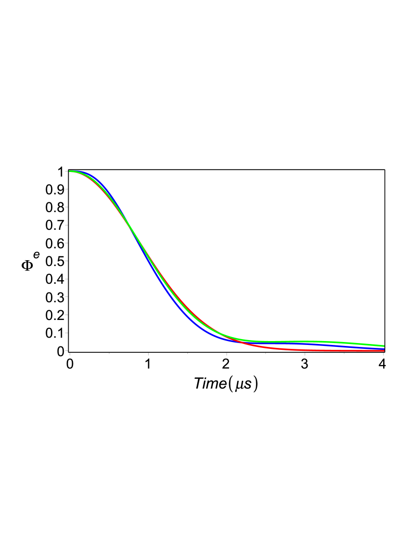
Figure 2: Sample A from YHNN . Echo decay, $\Phi^{e}(t)=\langle e^{i\psi(t)}\rangle$. The blue solid line is fit by two-fluctuator solution, $\langle e^{i\psi(t)}\rangle=\Phi_{1}^{e}(t)\Phi_{2}^{e}(t)$. The green solid line is the theoretical predictions of Ref. ZJR . Red solid line corresponds to the Gaussian decay, $\langle e^{i\psi(t)}\rangle=e^{-(\Gamma^{g}_{\varphi E}t)^{2}}$. The experimental data (not shown) are obtained for decoherence at value $\Delta n_{\phi}=0.0009$ (Fig. 4a, Ref. YHNN ).

In Fig. 2, we compare our theoretical predictions with the experimental data obtained for decoherence of a flux qubit with fluctuations of the external normalized flux, $n_{\phi}$ (sample A from YHNN ). To fit our theoretical results to the experimental curves, we set two cutoffs for ${1/f}$ noise as: $\gamma_{c}=0.5\;\rm\mu s^{-1}$ and $\gamma_{m}=0.5\;\rm s^{-1}$. Then, calculating the switching rate, $\gamma_{1}$ , we obtain $\gamma_{1}=0.04\;\rm\mu s^{-1}$. From Fig. 4c (in YHNN ), describing echo dephasing rate $\Gamma^{g}_{\varphi E}$ vs $\Delta n_{\phi}$, we extract $\Gamma^{g}_{\varphi E}=0.8\;\rm\mu s^{-1}$, and, then, using $(\ref{G2})$, we obtain $v_{1}=\sqrt{v^{2}_{n_{\phi}}}=4.92\;\rm\mu s^{-1}$. The parameters, $v_{2}$ and $\gamma_{0}$, are chosen by best fitting our curve to the experimental data. For the high-frequency noise we obtain the upper cutoff as $\gamma_{0}=4.25\;\rm\mu s^{-1}$. For the switching rate $\gamma_{2}$ this yields: $\gamma_{2}=1.2\;\rm\mu s^{-1}$. The amplitude $v_{2}$ we choose as $v_{2}=2.72\;\rm\mu s^{-1}$.

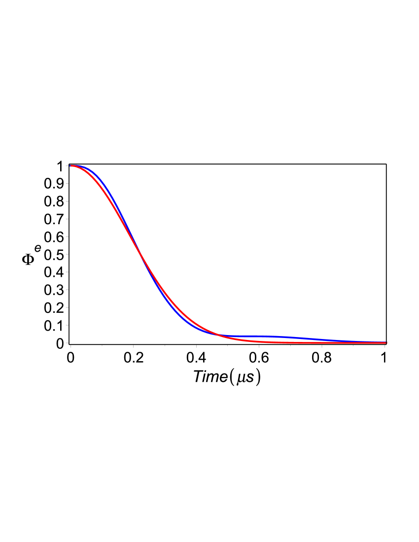
Figure 3: Sample B from YHNN . Echo decay, $\Phi^{e}(t)=\langle e^{i\psi(t)}\rangle$. The blue solid line is fit by the two fluctuator solution. The red solid line corresponds to the Gaussian decay $e^{-(\Gamma^{g}_{\varphi E}t)^{2}}$. The experimental data are obtained for decoherence for value $\Delta n_{\phi}=-0.0008$ (Fig. 4d, Ref. YHNN ).

In Fig. 3, we compare our theoretical predictions with the experimental data obtained for decoherence in a flux qubit with fluctuations of the external flux, $n_{\phi}$ (sample B from YHNN ). The fitting parameters obtained in the same way as for sample A are: $\gamma_{1}=0.04\;\rm\mu s^{-1}$ , $v_{1}=21\;\rm\mu s^{-1}$, $\gamma_{2}=5.75\;\rm\mu s^{-1}$, $v_{2}=12.45\;\rm\mu s^{-1}$ and $\Gamma^{g}_{\varphi E}=3.75\;\rm\mu s^{-1}$. In Figs. 2 and 3, the echo decay of the two fluctuator model (blue curves) resulted from both low and high frequency fluctuators.

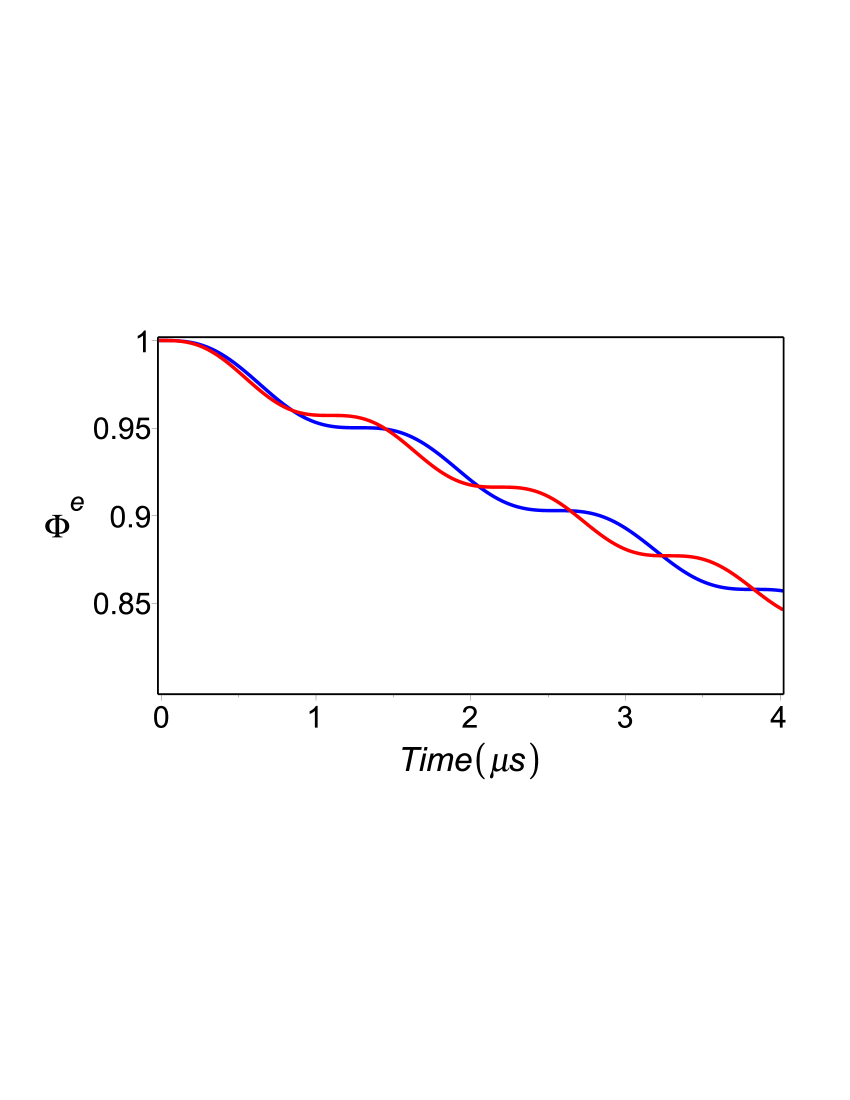
Figure 4: Suppression of $1/f$ noise in echo-decay experiment in a flux qubit at fluctuations of the external flux. The blue solid line corresponds to sample A, and the red solid line corresponds to sample B from Ref. YHNN .

In order to determine the contribution from only $1/f$ noise to this echo decay, we present in Fig. 4 the decay (for samples A and B) provided by only a slow effective fluctuator with the same parameters, $\gamma_{1}$ and $v_{1}$, as those indicated in Figs. 2 and 3. One can see from Fig. 4 that in both cases, a suppression of $1/f$ noise is up to $95\%$ in the time-interval, $(0-1\mu s)$.

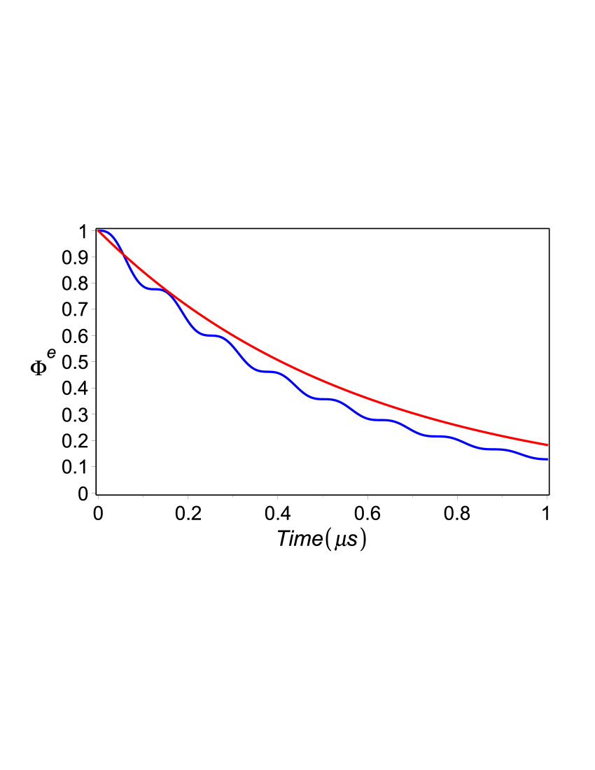
Figure 5: Echo decay, $\Phi^{e}(t)=\langle e^{i\psi(t)}\rangle$. The blue solid line is fit by the solution of the two-effective-fluctuators model, with the choice of $\gamma_{1}=0.04\rm MHz$, $v_{1}=10.5\rm MHz$, $\gamma_{2}=2\rm MHz$ and $v_{2}=50\rm MHz$. The red solid line corresponds to the exponential decay, $e^{-\Gamma_{\varphi E}t}$ with $\Gamma_{\varphi E}=1.7\rm MHz$. The experimental data are obtained for decoherence at value of SQUID bias current $I_{b}=-0.7\mu\rm A$ (sample A, Fig. 3c, Ref. YHNN ).

In Fig. 5, we compare our theoretical results for echo decay with the experimental data obtained for decoherence in a flux qubit for fluctuations of SQUID bias currents $I_{b}$ (sample A from YHNN ). In all considered cases, we find that our solutions based on two effective fluctuators better fit the experimental data than the theoretical description of the Gaussian approximation used in YHNN .

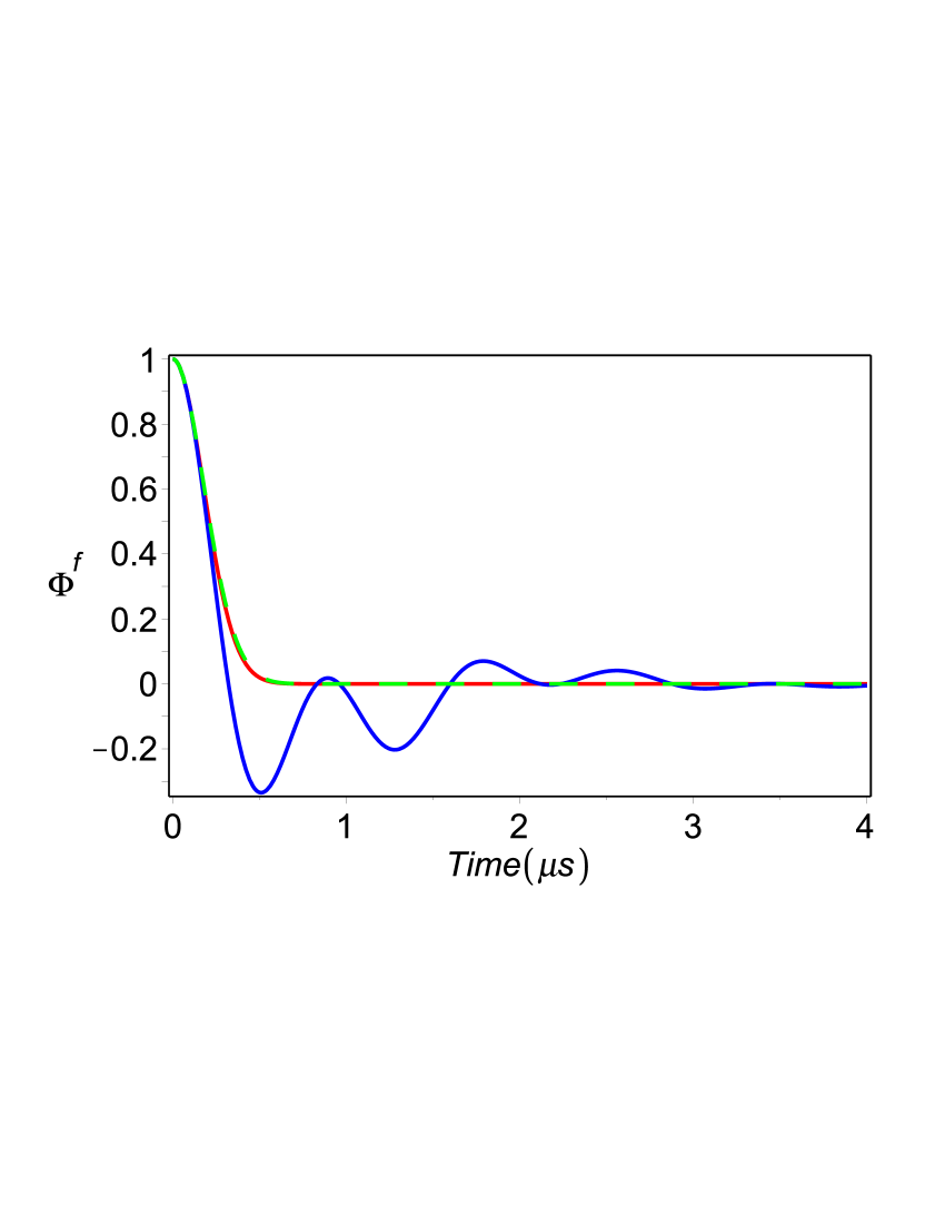
Figure 6: Sample A from YHNN . Free induction signal decay, $\Phi^{f}(t)=\langle e^{i\varphi(t)}\rangle$. Blue solid line fits to the two fluctuators solution, $\Phi^{f}(t)=\Phi_{1}^{f}(t)\Phi_{2}^{f}(t)$. Red solid line corresponds to the Gaussian decay, $\Phi^{f}=e^{-(\Gamma^{g}_{\varphi F}t)^{2}}$ with $\Gamma^{g}_{\varphi F}=3.97\;\rm\mu s^{-1}$. Green dashed line presents the Gaussian approximation for free decay, $\langle e^{i\varphi(t)}\rangle=e^{-(1/2)\langle\varphi^{2}(t)\rangle}$. (Data are taken from Ref. YHNN for decoherence at various flux biases $n_{\phi}$, sample A.)

We consider also free induction decay, and compare the obtained effective decoherence rate, $\Gamma^{g}_{\varphi F}$, with the experimental data and theoretical results of the Gaussian model ICJM ; YHNN . For free induction decay, the two-fluctuator solution is

$$\langle e^{i\varphi(t)}\rangle=\Phi^{f}_{1}(t)\Phi^{f}_{2}(t),$$ (85)

where $\Phi^{f}_{i}(t)$ $(i=1,2)$ are given by Eq. (77).

Expanding (85) into a Taylor series, we obtain

$$\langle e^{i\varphi(t)}\rangle=1-\frac{1}{2}(v_{1}^{2}+v_{2}^{2})t^{2}+\dots.$$ (86)

Then, comparing with the Gaussian decay, $e^{-(\Gamma^{g}_{\varphi F}t)^{2}}$, we obtain

$$\Gamma^{g}_{\varphi F}=\sqrt{\frac{1}{2}(v_{1}^{2}+v_{2}^{2})}.$$ (87)

Substituting $v_{1}=4.92\rm MHz$ and $v_{2}=2.72\rm MHz$ (sample A), we find $\Gamma^{g}_{\varphi F}=3.97\rm MHz$.

Computation for the sample A of the the ratio, $\Gamma^{g}_{\varphi F}/\Gamma^{g}_{\varphi E}$, yields $\Gamma^{g}_{\varphi F}/\Gamma^{g}_{\varphi E}\approx 4.96$. This is in a good agreement with the theoretical prediction, $\Gamma^{g}_{\varphi F}/\Gamma^{g}_{\varphi E}\lesssim 5$ ICJM , and with the estimate from the experimental data yielding a ratio between $4.5$ and $7.5$ YHNN .

IV.2.2 Gaussian approximation

In the Gaussian approximation, free induction signal decay is described by

$$\langle e^{i\varphi(t)}\rangle=e^{-(1/2)\langle\varphi^{2}(t)\rangle},$$ (88)

where $\langle{\varphi^{2}(t)}\rangle=\langle{\varphi_{1}^{2}(t)}\rangle+\langle{\varphi_{2}^{2}(t)}\rangle$, and $\langle\varphi_{n}^{2}(t)\rangle$ ($n=1,2$) is given by Eq. (212).

In Fig. 6, we compare the Gaussian approximation (green dashed line), the two-fluctuator solution (blue solid line) and the Gaussian decay (red solid line). As one can see, the Gaussian approximation and the Gaussian decay yield practically the same results. However, the two-fluctuator solution shows non-Gaussian oscillatory behavior.

We also considered the echo decay signal for the Sample A. Our theoretical results for echo decay follow from (57) and (58)

$$\langle e^{i\psi(t)}\rangle=e^{-(1/2)\langle{\psi^{2}(t)}\rangle},$$ (89)

where $\langle{\psi^{2}(t)}\rangle=\langle{\psi_{1}^{2}(t)}\rangle+\langle{\psi_{2}^{2}(t)}\rangle$, and $\langle\psi_{{n}}^{2}(t)\rangle$ (n=1,2) is given by Eq. (216)

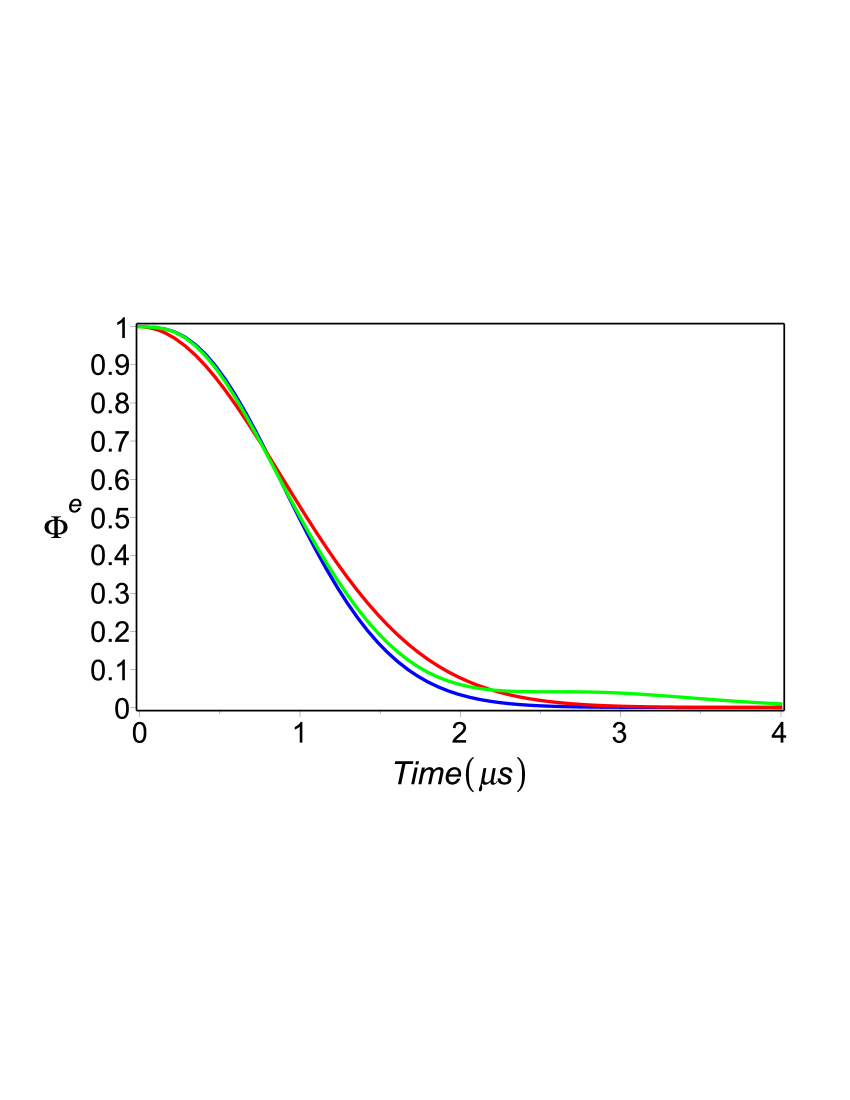
Figure 7: Sample A YHNN . Echo signal decay, $\Phi^{e}(t)=\langle e^{i\psi(t)}\rangle$. The blue solid line is fit by the Gaussian approximation, $\langle e^{i\psi(t)}\rangle=e^{-(1/2)\langle{\psi^{2}(t)}\rangle}$. Green solid line: two fluctuator solution, $\langle e^{i\psi(t)}\rangle=\Phi_{1}^{e}(t)\Phi_{2}^{e}(t)$. The red solid line corresponds to Gaussian decay, $\langle e^{i\psi(t)}\rangle=e^{-(\Gamma^{g}_{\varphi E}t)^{2}}$.

In Fig. 7, we present theoretical results (sample A) for echo decay for: the two-effective-fluctuator model (green curve); the Gaussian approximation (blue curve), and Gaussian decay used in [19] (red curve).

In Fig. 8, we compare the theoretical results for suppression of $1/f$ noise by slow fluctuators in the two-effective-fluctuator model and the Gaussian approximation. One can see that, up to $1\;\rm\mu s$, both descriptions give similar results. For times larger the 1 microsecond, the Gaussian approximation does not describe the suppression of $1/f$ noise, since fluctuators with $\gamma\approx\gamma_{c}$ dominate.

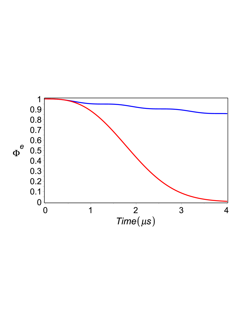
Figure 8: Suppression of $1/f$ noise in echo-decay experiment. The blue solid line corresponds to the two fluctuator solution with only slow fluctuators. The red solid line corresponds to the Gaussian approximation with slow fluctuators.

V Conclusions

The approach based on modeling of noisy environment by an ensemble of two-level systems (fluctuators) is widely used for quantum solid-state systems BGA ; GABS ; MSAM ; SSMM ; ICJM ; YBLA . Recent experiments with Josephson phase qubits CSMM ; SLHN ; APNY demonstrated the importance of noise of all frequencies in decoherence processes and stimulated theoretical discussions on the contributions of low- and high-frequencies fluctuators ICJM .

In this paper, we have discussed the SF model for continuous distribution of fluctuators to describe both, low- and high-frequency noise. We considered two approximations of our model: the Gaussian approximation and two-fluctuator approximation, and compared our theoretical predictions with the experimental results for decoherence of a superconducting flux qubit YHNN . We showed a good agreement between our theoretical model and experimental results.

We should emphasize that the two-fluctuator approximation leads to the non-Gaussian behavior in the signal decay. The non-Gaussian effects, yielding contribution to a particular behavior of the tail in the spin echo signal, are very strong for free induction signal decay. The main problem is that available experimental results on superconducting qubits (including those reported in Ref. YHNN ) may not have a good enough precision to distinguish Gaussian and non-Gaussian behavior. However, it is no doubt that the non-Gaussian behavior is relevant to many situations and can help to understand better the nature of noise and its action on the system under consideration.

Appendix A Some properties of random processes

A.1 Random telegraph process

In this section, we derive some useful formulae for the random telegraph process (RTP) defined by $\xi_{N}(t)=\sum^{N}_{i=1}\zeta_{i}(t)$ with the correlation function, $\chi_{N}(|t-t^{\prime}|)=\langle\xi_{N}(t)\xi_{N}(t^{\prime})\rangle$, given by

$$\chi_{N}(|t-t^{\prime}|)=\sum^{N}_{i=1}a^{2}_{i}e^{-2\gamma_{i}|t-t^{\prime}|}.$$ (90)

We assume that the RTP is described by $N$ uncorrelated fluctuators, $\zeta_{i}(t)$. Each fluctuator switches randomly between the values $-1$ and $1$ with the probability $1/2$, so that $\zeta^{2}_{i}(t)=a^{2}_{i}=\rm const$, and after averaging over the initial states of each fluctuator, the following correlation relations hold KV1 ; KV2 ; KV3

$$\langle{\zeta}_{i}(t)\rangle=0,$$ (91)

$$\langle{\zeta}_{i}(t){\zeta}_{j}(t^{\prime})\rangle=\delta_{ij}a^{2}_{i}e^{-2\gamma_{i}(t-t^{\prime})},\;t\geq t^{\prime},$$ (92)

$$M^{i}_{n}(t_{1},t_{2},\dots,t_{n})=a^{2}_{i}e^{-2\gamma_{i}|t_{1}-t_{2}|}M^{i}_{n-2}(t_{3},\dots,t_{n}),$$ (93)

where

$$M^{i}_{n}(t_{1},t_{2},\dots,t_{n})=\langle{\zeta}_{i}(t_{1})\dots\zeta_{i}(t_{n})\rangle,\quad t_{1}\geq t_{2}\geq\dots\geq t_{n}.$$ (94)

From Eqs. (91) - (93), a recursive formula follows

$$M^{N}_{n}(t_{1},t_{2},\dots,t_{n})=\chi_{N}(t_{1}-t_{2})M^{N}_{n-2}(t_{3},\dots,t_{n}),$$ (95)

where

$$M^{N}_{n}(t_{1},t_{2},\dots,t_{n})=\langle{\xi_{N}}(t_{1})\dots\xi_{N}(t_{n})\rangle,\quad t_{1}\geq t_{2}\geq\dots\geq t_{n}.$$ (96)

The RTP is conveniently described by the generating functional KV3 ,

$$\Phi_{N}[t;v(\tau)]=\Big{\langle}\exp\Big{\{}i\int\limits_{0}^{t}d\tau\xi_{N}(\tau)v(\tau)\Big{\}}\Big{\rangle}.$$ (97)

Applying Eq. (95) and using the Taylor expansion of Eq. (97), we obtain an exact integral equation for the generating functional $\Phi_{N}[t;v]$:

$$\Phi_{N}[t;v(\tau)]=1-\int\limits_{0}^{t}dt_{1}\int\limits_{0}^{t_{1}}dt_{2}\chi_{N}(t_{1}-t_{2})v(t_{1})v(t_{2})\Phi_{N}[t_{2};v(\tau)].$$ (98)

One can transform this integral equation into the integro-differential equation,

$$\frac{d}{dt}\Phi_{N}[t;v(\tau)]=-v(t)\int\limits_{0}^{t}dt_{1}\chi_{N}(t-t_{1})v(t_{1})\Phi_{N}[t_{1};v(\tau)]$$ (99)

Let $R[t;\xi_{N}(\tau)]$ be an arbitrary functional. Then, using Eq. (95) and a Taylor expansion in $\xi_{N}(\tau)$, one can show that the following correlation splitting formula holds:

$$\langle{\xi_{N}}(t_{1}){\xi_{N}}(t_{2})R[t;\xi_{N}(\tau)]\rangle=\chi_{N}(t_{1}-t_{2})\langle R[t;\xi_{N}(\tau)]\rangle,\;t_{1}\geq t_{2}\geq\tau.$$ (100)

To calculate the correlator $\langle{\xi_{N}}(t)R[t;\xi_{N}(\tau)]\rangle$ for $\tau\leq t$ we use the following relations KV3 :

$$\langle{\xi_{N}}(t)R[t;\xi_{N}(\tau)+\eta(\tau)]\rangle=\Big{\langle}{\xi_{N}}(t)\exp\Big{\{}\int\limits_{0}^{t}d\tau\xi_{N}(\tau)\frac{\delta}{\delta\eta(\tau)}\Big{\}}\Big{\rangle}R[t;\eta(\tau)],$$ (101)

where $\eta(\tau)$ is a deterministic function. With the help of Eq. (99), we obtain

$$\langle{\xi_{N}}(t)R[t;\xi_{N}(\tau)+\eta(\tau)]\rangle= \int\limits_{0}^{t}dt_{1}\chi_{N}(t-t_{1})\Big{\langle}\frac{\delta}{\delta\eta(t_{1})}\exp\Big{\{}\int\limits_{0}^{t_{1}}d\tau\xi_{N}(\tau\frac{\delta}{\delta\eta(\tau)}\Big{\}}\Big{\rangle}R[t;\eta(\tau)]$$

$$= \int\limits_{0}^{t}dt_{1}\chi_{N}(t-t_{1})\Big{\langle}\frac{\delta}{\delta\eta(t_{1})}R[t;\eta(\tau)+\xi_{N}(\tau)\Theta(t_{1}-\tau)]\Big{\rangle}.$$ (102)

Taking the limit $\eta\rightarrow 0$, we find

$$\langle{\xi_{N}}(t)R[t;\xi_{N}(\tau)]\rangle=\int\limits_{0}^{t}dt_{1}\chi_{N}(t-t_{1})\Big{\langle}\frac{\delta}{\delta\xi_{N}(\tau)}\tilde{R}[t,t_{1};\xi_{N}(\tau)]\Big{\rangle},$$ (103)

where

$$\tilde{R}[t,t_{1};\xi_{N}(\tau)]=R[t;\xi_{N}(\tau)\Theta(t_{1}-\tau+0)].$$ (104)

By differentiating (104) with respect to time $t$, we obtain

$$\frac{d}{dt}\langle{\xi_{N}}(t)R[t;\xi_{N}(\tau)]\rangle-\int\limits_{0}^{t}dt_{1}\frac{d}{dt}\chi_{N}(t-t_{1})\frac{\delta}{\delta\xi_{N}(\tau)}\Big{\langle}\tilde{R}[t,t_{1};\xi_{N}(\tau)]\Big{\rangle}=\Big{\langle}{\xi_{N}}(t)\frac{d}{dt}R[t;\xi_{N}(\tau)]\Big{\rangle}.$$ (105)

This formula generalizes the differential formula KV1 ; KV2 ; KV3

$$\Big{(}\frac{d}{dt}+2\gamma\Big{)}\langle{\zeta}(t)R[t;\zeta(\tau)]\rangle=\Big{\langle}{\zeta}(t)\frac{d}{dt}R[t;\zeta(\tau)]\Big{\rangle},$$ (106)

taking place for the RTP described by $\zeta(t)$ with switching rate, $\gamma$.

Theorem 1. For the random telegraph process, ${\xi_{N}}(t)$, the following relation holds:

$$\langle{\xi_{N}}(t^{\prime})R[t;\xi_{N}(\tau)]\rangle=\frac{\chi_{N}(t^{\prime}-t)}{\chi_{N}(0)}\langle{\xi_{N}}(t)R[t;\xi_{N}(\tau)]\rangle,\quad t^{\prime}\geq t,$$ (107)

where $R[t;\xi_{N}(\tau)]$ is an arbitrary functional.

Proof. Writing $\xi^{2}_{N}(t)$ as

$$\xi^{2}_{N}(t)=\sum\limits_{i=1}^{N}\zeta^{2}_{i}(t)+\sum\limits_{i\neq j}^{N}\zeta^{2}_{i}(t)\zeta^{2}_{j}(t),$$ (108)

we can employ the fact that $\zeta^{2}_{i}(t)=\rm const$ KV1 ; KV2 . Next, using the relation $\chi_{N}(0)=\sum\limits_{i=1}^{N}\xi^{2}_{i}(t)$, we obtain

$$\frac{\xi^{2}_{N}(t)}{\chi_{N}(0)}-\frac{1}{\chi_{N}(0)}\sum\limits_{i\neq j}^{N}\zeta_{i}(t)\zeta_{j}(t)=1.$$ (109)

Inserting $(\ref{A21})$ into the l.h.s. of Eq. (107), we find

$$\langle{\xi_{N}}(t^{\prime})R[t;\xi_{N}(\tau)]\rangle=\langle{\xi_{N}}(t^{\prime})\frac{\xi^{2}_{N}(t)}{\chi_{N}(0)}R[t;\xi_{N}(\tau)]\rangle-\frac{1}{\chi_{N}(0)}\sum\limits_{i\neq j}^{N}\langle\zeta_{i}(t)\zeta_{j}(t){\xi_{N}}(t^{\prime})R[t;\xi_{N}(\tau)]\rangle.$$ (110)

Then, applying (95), we obtain

$$\langle{\xi_{N}}(t^{\prime})R[t;\xi_{N}(\tau)]\rangle=\frac{\chi_{N}(t^{\prime}-t)}{\chi_{N}(0)}\langle\xi_{N}(t)R[t;\xi_{N}(\tau)]\rangle-\frac{1}{\chi_{N}(0)}\sum\limits_{i\neq j}^{N}\langle\zeta_{i}(t)\zeta_{j}(t)\rangle\langle{\xi_{N}}(t^{\prime})R[t;\xi_{N}(\tau)]\rangle,\quad t^{\prime}\geq t.$$ (111)

Since for, $i\neq j$, $\langle\zeta_{i}(t)\zeta_{j}(t)\rangle=0$, this yields

$$\langle{\xi_{N}}(t^{\prime})R[t;\xi_{N}(\tau)]\rangle=\frac{\chi_{N}(t^{\prime}-t)}{\chi_{N}(0)}\langle\xi_{N}(t)R[t;\xi_{N}(\tau)],\quad t^{\prime}\geq t.$$ (112)

Corollary. In the limit $N\rightarrow\infty$, one has

$$\langle{\xi}(t^{\prime})R[t;\xi(\tau)]\rangle=\frac{\chi(t^{\prime}-t)}{\chi(0)}\langle\xi(t)R[t;\xi(\tau)],\quad t^{\prime}\geq t.$$ (113)

where $\chi(t^{\prime}-t)=\lim_{N\rightarrow\infty}\chi_{N}(t^{\prime}-t)$.

A.2 Effective Random Process

We define the effective random telegraph process (ERP) for $N\gg 1$, as $\xi(t)=\lim_{N\rightarrow\infty}\xi_{N}(t)$, considering the continuous distribution of amplitudes and switching rates. The correlation function, $\chi(t)=\lim_{N\rightarrow\infty}\chi_{N}(t)$, can be written as

$$\chi(|t-t^{\prime}|)=\lim_{N\rightarrow\infty}\sum^{N}_{i=1}a^{2}_{i}e^{-2\gamma_{i}|t-t^{\prime}|}=\iint dw(\sigma,\gamma)\sigma^{2}e^{-2\gamma|t-t^{\prime}|},$$ (114)

where, $\sigma^{2}=\lim_{N\rightarrow\infty}Na^{2}$, and $dw(\sigma,\gamma)$, depends on the specific distribution functions of fluctuators on the amplitudes and switching rates. The main relations for the ERP can be obtained from the previous section by taking the limit $N\rightarrow\infty$. Below we present the most important formulae.

The generating functional for the ERP being defined as

$$\Phi[t;v(\tau)]=\Big{\langle}\exp\Big{\{}i\int\limits_{0}^{t}d\tau\xi(\tau)v(\tau)\Big{\}}\Big{\rangle}$$ (115)

satisfies the following integral equation:

$$\Phi[t;v(\tau)]=1-\int\limits_{0}^{t}dt_{1}\int\limits_{0}^{t_{1}}dt_{2}\chi(t_{1}-t_{2})v(t_{1})v(t_{2})\Phi[t_{2};v(\tau)].$$ (116)

One can transform Eq. (116) into the integro-differential equation,

$$\frac{d}{dt}\Phi[t;v(\tau)]=-v(t)\int\limits_{0}^{t}dt_{1}\chi(t-t_{1})v(t_{1})\Phi[t_{1};v(\tau)]$$ (117)

For an arbitrary functional $R[t;\xi(\tau)]$ the following correlation splitting formula holds:

$$\langle{\xi}(t_{1}){\xi}(t_{2})R[t;\xi(\tau)]\rangle=\chi(t_{1}-t_{2})\langle R[t;\xi(\tau)]\rangle,\;t_{1}\geq t_{2}\geq\tau.$$ (118)

Finally, the differentiation formula (105) takes the form

$$\frac{d}{dt}\langle{\xi}(t)R[t;\xi(\tau)]\rangle-\int\limits_{0}^{t}dt_{1}\frac{d}{dt}\chi(t-t_{1})\frac{\delta}{\delta\xi(\tau)}\Big{\langle}\tilde{R}[t,t_{1};\xi(\tau)]\Big{\rangle}=\Big{\langle}{\xi}(t)\frac{d}{dt}R[t;\xi(\tau)]\Big{\rangle}.$$ (119)

Relation to the Gaussian random process. We would like to mention here an important consequence of the central limit theorem concerning a relation between ERP and the Gaussian random process. Assume that for individual fluctuators the correlation relations are given by

$$\langle{\zeta}_{i}(t)\rangle=0,$$ (120)

$$\langle{\zeta}_{i}(t){\zeta}_{j}(t^{\prime})\rangle=\frac{\sigma^{2}}{N}\delta_{ij}e^{-2\gamma|t-t^{\prime}|}.$$ (121)

Then, for $N\rightarrow\infty$, the ERP, defined by $\xi_{N}(t)$, becomes a Gaussian Markovian process with an exponential correlation function KV1 ; KV3

$$\langle{\xi}(t){\xi}(t^{\prime})\rangle=\sigma^{2}e^{-2\gamma|t-t^{\prime}|},$$ (122)

where $\xi(t)=\lim_{N\rightarrow\infty}\xi_{N}(t)$. Thus, the $N$-fluctuator RTP, with the same switching rates, $\gamma$, and the amplitudes, $\sigma^{2}/N$, for a finite number, $N$, is an approximation of a Gaussian Markovian process.

Appendix B Stochastic differential equations

We consider a system of first-order stochastic differential equations

$$\frac{d}{dt}{\mathbf{x}}(t)=\hat{A}(t){\mathbf{x}}(t)+\xi(t)\hat{B}(t){\mathbf{x}}(t),\;{\mathbf{x}}(0)={\mathbf{x}}_{0},$$ (123)

where $\xi(t)$ describes ERP, so that $\langle{\xi}(t)\xi(t^{\prime})\rangle=\chi(t-t^{\prime})$ $(t\geq t^{\prime})$ and

$$\chi(|t-t^{\prime}|)=\int dw(\sigma,\gamma)\sigma^{2}e^{-2\gamma|t-t^{\prime}|}.$$ (124)

In what follows we study two approximations leading to a closed system of differential equations for averaged variables: (i) The effective fluctuator approximation and (ii) the Gaussian approximation.

B.1 Gaussian approximation

In the interaction picture, we introduce the new variable $\tilde{\mathbf{x}}(t)=U^{-1}(t){\mathbf{x}}(t)$, where

$$U(t)=T\Big{(}e^{\int\limits_{0}^{t}\hat{A}(t^{\prime})dt^{\prime}}\Big{)}\tilde{\mathbf{x}}(t),$$ (125)

with a T-ordered exponential on the r.h.s. For $\tilde{\mathbf{x}}(t)$, Eq. (123) takes the form

$$\frac{d}{dt}\tilde{\mathbf{x}}(t)=i\xi(t)\hat{\tilde{B}}(t)\tilde{\mathbf{x}}(t),\;\tilde{\mathbf{x}}(0)={\mathbf{x}}_{0},$$ (126)

where we set $i\hat{\tilde{B}}(t)=U^{-1}(t)\hat{B}(t)U(t)$. Eq. (126) can be recast as

$$\frac{d}{dt}\tilde{\mathbf{x}}(t)=i\hat{\tilde{B}}(t)\xi(t)\tilde{\mathbf{x}}(0)-\hat{\tilde{B}}(t)\int\limits_{0}^{t}\xi(t)\xi(t^{\prime})\hat{\tilde{B}}(t^{\prime}),\tilde{\mathbf{x}}(t^{\prime})dt^{\prime}.$$ (127)

After averaging over ERP, we obtain the following integro-differential equation

$$\frac{d}{dt}\langle\tilde{\mathbf{x}}(t)\rangle=-\hat{\tilde{B}}(t)\int\limits_{0}^{t}\chi(t-t^{\prime})\hat{\tilde{B}}(t^{\prime})\langle\tilde{\mathbf{x}}(t^{\prime})\rangle dt^{\prime}.$$ (128)

For practical purposes, Eq. (128) is not very useful. However for some reasonable assumptions, it can be simplified. First, employing (128) one can write

$$\langle\tilde{\mathbf{x}}(t^{\prime})\rangle=\langle\tilde{\mathbf{x}}(t)\rangle-\int^{t^{\prime}}_{t}dt^{\prime}\hat{\tilde{B}}(t^{\prime})\int\limits_{0}^{t^{\prime\prime}}\chi(t^{\prime}-t^{\prime\prime})\hat{\tilde{B}}(t^{\prime\prime})\langle\tilde{\mathbf{x}}(t^{\prime})\rangle d{t^{\prime\prime}}.$$ (129)

Then, inserting (129) into Eq. (128) we obtain

$$\frac{d}{dt}\langle\tilde{\mathbf{x}}(t)\rangle=-\hat{\tilde{B}}(t)\int\limits_{0}^{t}\chi(t-t^{\prime})\hat{\tilde{B}}(t^{\prime})dt^{\prime}\langle\tilde{\mathbf{x}}(t)\rangle+{\mathcal{O}}(\parallel\hat{\tilde{B}}\parallel^{4}).$$ (130)

Considering the last term at the r.h.s. of Eq. (123) as a perturbation, one can approximate Eq. (128) as follows:

$$\frac{d}{dt}\langle\tilde{\mathbf{x}}(t)\rangle=-\hat{\tilde{B}}(t)\int\limits_{0}^{t}\chi(t-t^{\prime})\hat{\tilde{B}}(t^{\prime})dt^{\prime}\langle\tilde{\mathbf{x}}(t)\rangle.$$ (131)

Its formal solution can be written as

$$\langle\tilde{\mathbf{x}}(t)\rangle=T\Big{\{}\exp\Big{(}-\int\limits_{0}^{t}\hat{\tilde{B}}(t^{\prime})dt^{\prime}\int\limits_{0}^{t^{\prime}}\chi(t^{\prime}-t^{\prime\prime})\hat{\tilde{B}}(t^{\prime\prime})dt^{\prime\prime}\Big{)}\Big{\}}\langle\tilde{\mathbf{x}}(0)\rangle$$

$$=T\Big{\{}\exp\Big{(}-\frac{1}{2}\int\limits_{0}^{t}\int\limits_{0}^{t}\hat{\tilde{B}}(t^{\prime})\chi(t^{\prime}-t^{\prime\prime})\hat{\tilde{B}}(t^{\prime\prime})dt^{\prime}dt^{\prime\prime}\Big{)}\Big{\}}\langle\tilde{\mathbf{x}}(0)\rangle.$$ (132)

As can be seen, it has the form of solution for the Gaussian random process KV1 ; KV2 ; KV3 .

Returning to $\langle{\mathbf{x}}(t)\rangle$, we obtain the first-order differential equation

$$\frac{d}{dt}\langle{\mathbf{x}}(t)\rangle=\hat{A}(t)\langle{\mathbf{x}}(t)\rangle+\hat{B}(t)\hat{V}(t)\langle{\mathbf{x}}(t)\rangle,$$ (133)

where

$$\hat{V}(t)=\int_{0}^{t}dt^{\prime}\chi(t-t^{\prime})U(t)\hat{\tilde{B}}(t^{\prime})U^{-1}(t).$$ (134)

As an illustrative example, let us consider the following stochastic differential equation:

$$\frac{d}{dt}{x}(t)=i{A}{x}(t)+i{v}\xi(t){x}(t),$$ (135)

with $A$ and $v$ being $\rm const$. Its solution can be written as follows:

$$\langle{x}(t)\rangle=e^{i\varphi_{0}(t)}\langle e^{i\varphi(t)}\rangle\langle{x}(0)\rangle,$$ (136)

where $\varphi_{0}(t)=At$ is the regular part, and $\varphi(t)=v\int\limits_{0}^{t}\chi(t-t^{\prime})dt^{\prime}$ is the stochastic phase accumulated at time $t$.

In the Gaussian approximation, we find that the average $\langle{x}(t)\rangle$ satisfies the differential equation

$$\frac{d}{dt}\langle{x}(t)\rangle=i{A}\langle{x}(t)\rangle-{v^{2}}\Big{(}\int\limits_{0}^{t}\chi(t-t^{\prime})dt^{\prime}\Big{)}\langle{x}(t)\rangle.$$ (137)

The solution of Eq.(137) is given by

$$\langle{x}(t)\rangle=\langle e^{i\varphi_{0}(t)}\rangle e^{-\kappa(t)}\langle e^{i\varphi(0)}\rangle,$$ (138)

where

$$\kappa(t)=v^{2}\int\limits_{0}^{t}dt^{\prime}\int\limits_{0}^{t^{\prime}}\chi(t-t^{\prime})dt^{\prime\prime}=\frac{1}{2}v^{2}\int\limits_{0}^{t}\int\limits_{0}^{t}\chi(|t-t^{\prime}|)dt^{\prime}dt^{\prime\prime}=\frac{1}{2}\langle\varphi^{2}(t)\rangle.$$ (139)

From here and (136), it follows that the decay law for $\langle e^{i\varphi(t)}\rangle$ is the Gaussian,

$$\langle e^{i\varphi(t)}\rangle=e^{-\langle\varphi^{2}(t)\rangle/2}.$$ (140)

This agrees with the general conclusions made in this section.

B.2 Two-effective-fluctuator approximation

Averaging Eq. (123) over the ERP, we obtain

$$\frac{d}{dt}\langle{\mathbf{x}}(t)\rangle=\hat{A}(t)\langle{\mathbf{x}}(t)\rangle+\hat{B}(t)\langle{\mathbf{X}}_{\xi}(t)\rangle,$$ (141)

where $\langle{\mathbf{X}}_{\xi}(t)\rangle=\langle\xi(t){\mathbf{x}}(t)\rangle$. Using (123), and taking into account that $\langle{\mathbf{X}}_{\xi}(0)\rangle=0$, we obtain

$$\langle{\mathbf{X}}_{\xi}(t)\rangle=\int\limits_{0}^{t}\frac{\chi(t-t^{\prime})}{\chi(0)}\hat{A}(t^{\prime})\langle{\mathbf{X}}_{\xi}(t^{\prime})\rangle dt^{\prime}+\int\limits_{0}^{t}\chi(t-t^{\prime})\hat{B}(t^{\prime})\langle{\mathbf{x}}(t^{\prime})\rangle dt^{\prime}.$$ (142)

Taking the derivative on both sides of Eq. (142), we obtain

$$\frac{d}{dt}\langle{\mathbf{X}}_{\xi}(t)\rangle= \hat{A}(t)\langle{\mathbf{X}}_{\xi}(t)\rangle+\chi(0)\hat{B}(t)\langle{\mathbf{x}}(t)\rangle$$

$$+\frac{1}{\chi(0)}\int\limits_{0}^{t}\frac{\partial\chi(t-t^{\prime})}{\partial t}\Big{(}\hat{A}(t^{\prime})\langle{\mathbf{X}}_{\xi}(t^{\prime})\rangle^{\prime}+\chi(0)\hat{B}(t^{\prime})\langle{\mathbf{x}}(t^{\prime})\rangle\Big{)}dt^{\prime}.$$ (143)

Finally, we obtain the following closed system of integro-differential equations:

$$\frac{d}{dt}\langle{\mathbf{x}}(t)\rangle= \hat{A}(t)\langle{\mathbf{x}}(t)\rangle+\hat{B}(t)\langle{\mathbf{X}}_{\xi}(t)\rangle,$$ (144)

$$\frac{d}{dt}\langle{\mathbf{X}}_{\xi}(t)\rangle= \hat{A}(t)\langle{\mathbf{X}}_{\xi}(t)\rangle+\chi(0)\hat{B}(t)\langle{\mathbf{x}}(t)\rangle$$

$$+\frac{1}{\chi(0)}\int\limits_{0}^{t}\frac{\partial\chi(t-t^{\prime})}{\partial t}\Big{(}\hat{A}(t^{\prime})\langle{\mathbf{X}}_{\xi}(t^{\prime})\rangle+\chi(0)\hat{B}(t^{\prime})\langle{\mathbf{x}}(t^{\prime})\rangle\Big{)}dt^{\prime}.$$ (145)

In this section, we consider the system of Eqs. (144), (145) in the approximation that the ERP can be approximated by a random telegraph process with the correlation function, $\chi^{\ast}(|t-t^{\prime}|)$,

$$\chi(|t-t^{\prime}|)=\int dw(\sigma,\gamma)\sigma^{2}e^{-2\gamma|t-t^{\prime}|}\approx\chi^{\ast}(|t-t^{\prime}|)={a^{*}}^{2}e^{-2\gamma^{*}|t-t^{\prime}|},$$ (146)

where the time-independent parameters, $a^{*}$ and $\gamma^{*}$ (the effective amplitude and the switching rate) are defined by the following expressions: ${a^{*}}^{2}=\chi(0)$ and $\gamma^{*}=-(1/2)\partial\ln\chi(t)/\partial t|_{t=0}$.

To proceed, consider Eq.(145) rewritten as

$$\frac{d}{dt}\langle{\mathbf{X}}_{\xi}(t)\rangle= \hat{A}(t)\langle{\mathbf{X}}_{\xi}(t)\rangle+\chi(0)\hat{B}(t)\langle{\mathbf{x}}(t)\rangle$$

$$+\int\limits_{0}^{t}\frac{\partial\ln\chi(t-t^{\prime})}{\partial t}\chi(t-t^{\prime})\Big{(}\frac{1}{\chi(0)}\hat{A}(t^{\prime})\langle{\mathbf{X}}_{\xi}(t^{\prime})\rangle+\hat{B}(t^{\prime})\langle{\mathbf{x}}(t^{\prime})\rangle\Big{)}dt^{\prime}.$$ (147)

Usually $\ln\chi(t)$ is a slowly-changing function. Then, replacing $\partial\ln\gamma(t-t^{\prime})/\partial t$ by its value at time, $t=t^{\prime}$, one can approximate the integral on the right side of Eq. (147) as follows:

$$\int\limits_{0}^{t}\frac{\partial\ln\chi(t-t^{\prime})}{\partial t}\chi(t-t^{\prime})\Big{(}\frac{1}{\chi(0)}\hat{A}(t^{\prime})\langle{\mathbf{X}}_{\xi}(t^{\prime})\rangle^{\prime}+\hat{B}(t^{\prime})\langle{\mathbf{x}}(t^{\prime})\rangle\Big{)}dt^{\prime}$$

$$\approx\frac{\partial\ln\chi(t-t^{\prime})}{\partial t}\Big{|}_{t=t^{\prime}}\int\limits_{0}^{t}\chi(t-t^{\prime})\Big{(}\frac{1}{\chi(0)}\hat{A}(t^{\prime})\langle{\mathbf{X}}_{\xi}(t^{\prime})\rangle+\hat{B}(t^{\prime})\langle{\mathbf{x}}(t^{\prime})\rangle\Big{)}dt^{\prime}.$$ (148)

Inserting (148) into (147), and employing (142) we obtain

$$\frac{d}{dt}\langle{\mathbf{X}}_{\xi}(t)\rangle=\hat{A}(t)\langle{\mathbf{X}}_{\xi}(t)\rangle-2\gamma^{*}\langle{\mathbf{X}}_{\xi}(t)\rangle+{a^{\ast}}^{2}\hat{B}(t)\langle{\mathbf{x}}(t)\rangle,$$ (149)

where $\gamma^{*}=-(1/2)\partial\ln\chi(t)/\partial t|_{t=0}$ and ${a^{\ast}}^{2}=\chi(0)$. Next, combining (141) and (149), instead of a system of integro-differential equations, we obtain a closed system of first-order differential equations

$$\frac{d}{dt}\langle{\mathbf{x}}(t)\rangle=\hat{A}(t)\langle{\mathbf{x}}(t)\rangle+\hat{B}(t)\langle{\mathbf{X}}_{\xi}(t)\rangle,\quad\langle{\mathbf{x}}(0)\rangle={\mathbf{x}}(0),$$ (150)

$$\frac{d}{dt}\langle{\mathbf{X}}_{\xi}(t)\rangle+2\gamma^{*}\langle{\mathbf{X}}_{\xi}(t)\rangle=\hat{A}(t)\langle{\mathbf{X}}_{\xi}(t)\rangle+{a^{\ast}}^{2}\hat{B}(t)\langle{\mathbf{x}}(t)\rangle,\quad\langle{\mathbf{X}}_{\xi}(0)\rangle=0.$$ (151)

This system of differential equations describes RTP with the amplitude $a^{\ast}$, switching rate $\gamma^{*}$ and the correlation function KV3

$$\chi^{\ast}(|t-t^{\prime}|)={a^{*}}^{2}e^{-2\gamma^{*}|t-t^{\prime}|}.$$ (152)

In Fig. 9, we compare the exact correlation functions,

$$\chi_{1}(\tau)=\sigma^{2}_{1}A_{1}(E_{1}(2\gamma_{m}\tau)-E_{1}(2\gamma_{c}\tau)),$$ (153)

$$\chi_{2}(\tau)=\sigma^{2}_{2}A_{2}\bigg{(}\frac{E_{2}(2\gamma_{c}\tau)}{\gamma_{c}}-\frac{E_{2}(2\gamma_{0}\tau)}{\gamma_{0}}\bigg{)},$$ (154)

with their approximated expressions, $\chi_{n}\approx\sigma^{2}_{n}\exp(-2\gamma_{n}t)$ given by (63). The choice of parameters, $\gamma_{m}$ and $\gamma_{c}$, was motivated by the range of frequencies for $1/f$ noise. The parameter, $\gamma_{0}$, was chosen to better fit both exact and approximate correlation functions. Note, that the correlation function in (63) which describes the low frequency noise, $\chi_{1}$, is not very sensitive to variations of the parameter, $\gamma_{m}$. Further, when fitting the experimental data, the parameters, $\gamma_{m}$ and $\gamma_{c}$, were essentially the same as in Fig. 9. As can be seen, the approximation (146) describes the behavior of the exact correlation functions reasonably well for the region of parameters which we use.

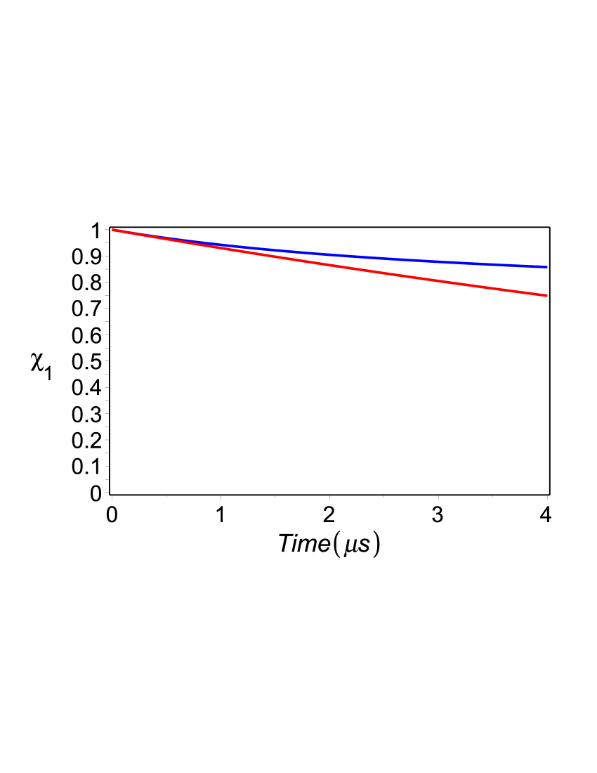
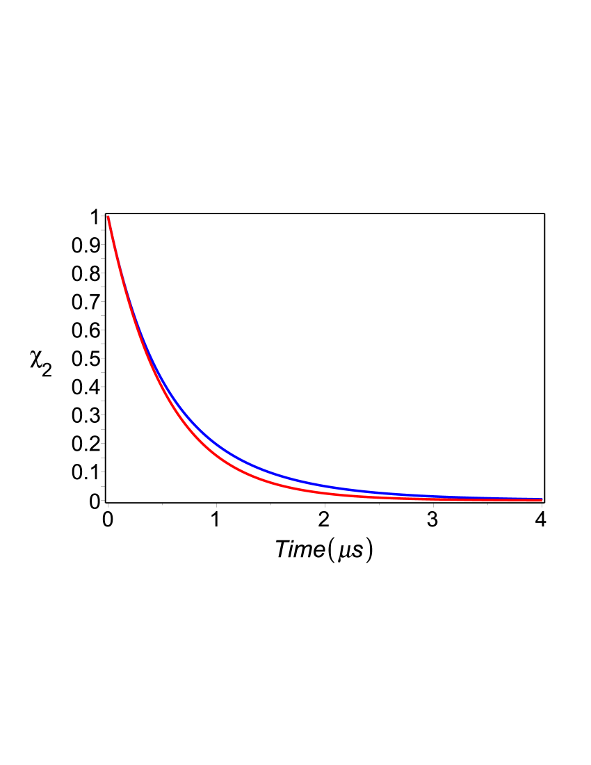
Figure 9: Correlation functions, $\chi_{n}(t)$, (blue line) and exponential correlation functions, $\chi_{n}(t)=\exp(-2\gamma_{n}t)$, (red line). Upper panel: Low-frequency noise defined by $\chi_{1}(t)$ ($\gamma_{m}=0.5\;\rm s^{-1}$, $\gamma_{c}=0.5\;\rm\mu s^{-1}$). There is good agreement up to $\sim 2\mu s$. Bottom panel: High- frequency noise defined by $\chi_{2}(t)$ ($\gamma_{c}=0.5\;\rm\mu s^{-1}$, $\gamma_{0}=2\;\rm\mu s^{-1}$). In all cases $\sigma_{n}^{2}=1$.

The system of Eqs. (150), (151) approximately describes an ERP by RTP defined by a single fluctuator. Below, we will describe a model with two effective (low- and high-frequency) fluctuators. The advantage of this approach is that we calculate in a straightforward way the coefficients $a^{*}$ and $\gamma^{*}$.

Two-effective-fluctuators model

Let us consider the same system of first-order stochastic differential equations as above

$$\frac{d}{dt}{\mathbf{x}}(t)=\hat{A}(t){\mathbf{x}}(t)+\xi(t)\hat{B}(t){\mathbf{x}}(t),\;{\mathbf{x}}(0)={\mathbf{x}}_{0},$$ (155)

with the RTP described by two uncorrelated fluctuators, $\zeta_{1}(t)$ and 2$\zeta_{2}(t)$, so that $\xi(t)=\zeta_{2}(t)+\zeta_{2}(t)$, and

$$\langle{\zeta}_{i}(t)\rangle=0,$$ (156)

$$\langle{\zeta}_{i}(t){\zeta}_{j}(t^{\prime})\rangle=\delta_{ij}a^{2}_{i}e^{-2\gamma_{i}|t-t^{\prime}|},\quad i=1,2.$$ (157)

We set $\langle{\mathbf{X}}_{1}(t)\rangle=\langle\zeta_{1}(t){\mathbf{x}}(t)\rangle$, $\langle{\mathbf{X}}_{2}(t)\rangle=\langle\zeta_{2}(t){\mathbf{x}}(t)\rangle$ and $\langle{\mathbf{X}}_{12}(t)\rangle=\langle\zeta_{1}(t)\zeta_{2}(t){\mathbf{x}}(t)\rangle$. Applying the formulae of differentiation for an RTP KV1 ; KV2 ; KV3 , we obtain the following system of differential equations for averaged variables:

$$\frac{d}{dt}\langle{\mathbf{x}}(t)\rangle=\hat{A}(t)\langle{\mathbf{x}}(t)\rangle+\hat{B}(t)(\langle{\mathbf{X}}_{1}(t)\rangle+\langle{\mathbf{X}}_{2}(t)\rangle),$$

$$\frac{d}{dt}\langle{\mathbf{X}}_{1}(t)\rangle=-2\gamma_{1}\langle{\mathbf{X}}_{1}(t)\rangle+\hat{A}(t)\langle{\mathbf{X}}_{1}(t)\rangle+\hat{B}(t)(\langle{\mathbf{X}}_{12}(t)\rangle+a^{2}_{1}\langle{\mathbf{x}}(t)\rangle),$$

$$\frac{d}{dt}\langle{\mathbf{X}}_{2}(t)\rangle=-2\gamma_{2}\langle{\mathbf{X}}_{1}(t)\rangle+\hat{A}(t)\langle{\mathbf{X}}_{2}(t)\rangle+\hat{B}(t)(\langle{\mathbf{X}}_{12}(t)\rangle+a^{2}_{2}\langle{\mathbf{x}}(t)\rangle),$$

$$\frac{d}{dt}\langle{\mathbf{X}}_{12}(t)\rangle=-2(\gamma_{1}+\gamma_{2})\langle{\mathbf{X}}_{12}(t)\rangle+\hat{A}(t)\langle{\mathbf{X}}_{12}(t)\rangle+\hat{B}(t)(a^{2}_{2}\langle{\mathbf{X}}_{1}(t)\rangle+a^{2}_{1}\langle{\mathbf{X}}_{2}(t)\rangle).$$ (158)

Appendix C Properties of the correlation functions

We consider a family of random variables and distributions, $\{\xi_{n}(t),dw_{n}(\sigma,\gamma)\}$, in which each $\xi_{n}(t)$ describes an independent ERP: $\langle\xi_{m}(t)\xi_{n}(t^{\prime})\rangle=0$ $(m\neq n)$. Then, the total correlation function is a sum of the partial correlation functions and $\chi(|t-t^{\prime}|)=\sum_{n}\chi_{n}(|t-t^{\prime}|)$, can be written as

$$\chi(|t-t^{\prime}|)=\sum_{n}\iint dw_{n}(\sigma,\gamma)\sigma^{2}e^{-2\gamma|t-t^{\prime}|}.$$ (159)

We define the distribution function, $dw_{n}(\sigma,\gamma)$, as

$$dw_{n}(\sigma,\gamma)=\delta(\sigma-\sigma_{n}){\mathcal{P}}_{n}(\gamma)d\sigma d\gamma,$$ (160)

where, $\sigma_{n}$, is a some typical value of the amplitude, and

$${\mathcal{P}}_{n}(\gamma)d\gamma=A_{n}\Theta(\gamma_{c_{n}}-\gamma)\Theta(\gamma-\gamma_{m_{n}})\displaystyle\frac{d\gamma}{\gamma^{n}},\quad n=1,2,\dots,$$ (161)

here, $\Theta(x)$, denotes the step-function, $\gamma_{m_{n}}$ and $\gamma_{c_{n}}$ are the lower and upper switching rates, respectively. The normalization constant given by,

$$A_{n}=\left\{\begin{array}[]{ll}\displaystyle\frac{1}{\ln(\gamma_{c_{1}}/\gamma_{m_{1}})},&n=1\\ &\\ \displaystyle\frac{(n-1)\gamma^{n-1}_{m_{n}}}{(1-\gamma^{n-1}_{m_{n}}/\gamma^{n-1}_{c_{n}})},&n\neq 1\end{array}\right.,$$ (165)

is obtained from the normalization condition, $\int dw_{n}(\sigma,\gamma)=1$.

Inserting (161) into (159), we obtain,

$$\chi_{n}(|t-t^{\prime}|)={\sigma}_{n}^{2}\iint{\mathcal{P}}_{n}(\gamma)d\gamma e^{-2\gamma|t-t^{\prime}|}.$$ (166)

From (166) it follows that $\sigma^{2}=\chi(0)$, and straightforward computation yields,

$$\chi_{n}(\tau)={\sigma^{2}_{n}A_{n}}\Bigg{(}\frac{E_{n}(2\gamma_{m_{n}}\tau)}{\gamma_{m_{n}}^{n-1}}-\frac{E_{n}(2\gamma_{c_{n}}\tau)}{\gamma_{c_{n}}^{n-1}}\Bigg{)},$$ (167)

where $E_{n}(z)$ denotes the Exponential integral abr .

It is convenient to describe each noise source by its spectral density,

$$S_{n}(\omega)=\frac{1}{\pi}\int\limits_{0}^{\infty}\chi_{n}(\tau)\cos(\omega\tau)d\tau,$$ (168)

and, as it can be easily seen, $\sigma^{2}_{n}=2\int\limits_{0}^{\infty}S_{n}(\omega)d\omega$. Employing Eqs. (159) and 168), one can obtain the following integral representation for $S_{n}(\omega)$:

$$S_{n}(\omega)=\frac{1}{\pi}\int\frac{2\gamma\sigma^{2}}{4\gamma^{2}+\omega^{2}}\,dw_{n}(\sigma,\gamma),$$ (169)

where

$$S_{L}(\Omega)=\frac{1}{\pi}\frac{2\gamma\sigma^{2}}{4\gamma^{2}+\omega^{2}}$$ (170)

is the Lorentzian spectral density of the fluctuator with the amplitude $\sigma$ and switching rate $\gamma$ BGA .

Performing the integration in Eq. (168), we obtain for $n>2$

$$S_{n}(\omega)=\frac{1}{\pi}\sigma^{2}_{n}A_{n}2^{n-1}\sum^{[(n+1)/2]}_{k=1}\frac{(-1)^{k+1}}{(n-2k)\omega^{2k}}\bigg{(}\frac{1}{b_{n}^{n-2k}}-\frac{1}{c_{n}^{n-2k}}\bigg{)}$$ (171)

$$+\frac{1}{\pi\omega^{n}}A_{n}\sigma^{2}_{n}2^{n-1}\left\{\begin{array}[]{ll}\displaystyle\frac{1}{2}\ln\bigg{(}\frac{1+({\omega}/{b_{n}})^{2}}{1+({\omega}/{c_{n}})^{2}}\bigg{)},&n=2p,\\ &\\ \displaystyle\arctan\Big{(}\frac{\omega}{b_{n}}\Big{)}-\arctan\Big{(}\frac{\omega}{c_{n}}\Big{)},&n=2p+1,\end{array}\right.$$ (175)

where $b_{n}=2\gamma_{m_{n}}$ and $c_{n}=2\gamma_{c_{n}}$. For $n=1,2$, the computation yields

$$S_{1}(\omega)=\frac{\sigma^{2}_{1}A_{1}}{\pi\omega}\bigg{(}\arctan\Big{(}\frac{\omega}{b_{1}}\Big{)}-\arctan\Big{(}\frac{\omega}{c_{1}}\Big{)}\bigg{)},$$ (176)

$$S_{2}(\omega)=\frac{\sigma^{2}_{2}A_{2}}{\pi\omega^{2}}\ln\bigg{(}\frac{1+({\omega}/{b_{2}})^{2}}{1+({\omega}/{c_{2}})^{2}}\bigg{)}$$ (177)

We impose on the distribution functions ${\mathcal{P}}_{1}(\gamma)$ and ${\mathcal{P}}_{2}(\gamma)$ boundary conditions at the point $\gamma=\gamma_{c}$, so that $\gamma_{m_{2}}=\gamma_{c_{1}}$. Further, we denote $\gamma_{m}=\gamma_{m_{1}}$, $\gamma_{c}=\gamma_{c_{1}}$, and $\gamma_{0}=\gamma_{c_{2}}$ $(\gamma_{m}<\gamma_{c}<\gamma_{0})$. Using these notations, we obtain

$$S_{1}(\omega)=\frac{\sigma^{2}_{1}A_{1}}{\pi\omega}\bigg{(}\arctan\Big{(}\frac{\omega}{2\gamma_{m}}\Big{)}-\arctan\Big{(}\frac{\omega}{2\gamma_{c}}\Big{)}\bigg{)},$$ (178)

$$S_{2}(\omega)=\frac{\sigma^{2}_{2}A_{2}}{\pi\omega^{2}}\ln\bigg{(}\frac{1+\omega^{2}/4\gamma_{c}^{2}}{1+\omega^{2}/4\gamma_{0}^{2}}\bigg{)},$$ (179)

This yields the following asymptotic behavior of $S_{1}(\omega)$ and $S_{2}(\omega)$:

$$S_{1}(\omega)\approx\left\{\begin{array}[]{ll}\displaystyle\frac{\sigma^{2}_{1}}{2\pi\gamma_{m}\ln(\gamma_{c}/\gamma_{m})}\bigg{(}1-\frac{\gamma_{m}}{\gamma_{c}}\bigg{)},&\omega\ll 2\gamma_{m},\\ \\ \displaystyle\frac{\sigma^{2}_{1}}{2\omega\ln(\gamma_{c}/\gamma_{m})},&2\gamma_{m}\ll\omega\ll 2\gamma_{c},\\ \\ \displaystyle\frac{2\sigma^{2}_{1}\gamma_{c}(1-\gamma_{m}/\gamma_{c})}{\pi\omega^{2}\ln(\gamma_{c}/\gamma_{m})},&\omega\gg 2\gamma_{c},\end{array}\right.$$ (185)

and

$$S_{2}(\omega)\approx\left\{\begin{array}[]{ll}\displaystyle\frac{\sigma^{2}_{2}}{4\pi\gamma_{c}}\bigg{(}1+\frac{\gamma_{c}}{\gamma_{0}}\bigg{)},&\omega\ll 2\gamma_{c}<2\gamma_{0},\\ \\ \displaystyle\frac{2\sigma^{2}_{2}\gamma_{c}}{\pi(1-\gamma_{c}/\gamma_{0})\omega^{2}}\ln\bigg{(}\frac{\omega}{2\gamma_{c}}\bigg{)},&2\gamma_{c}\ll\omega\ll 2\gamma_{0},\\ \\ \displaystyle\frac{2\sigma^{2}_{2}\gamma_{c}}{\pi(1-\gamma_{c}/\gamma_{0})\omega^{2}}\ln\bigg{(}\frac{\gamma_{0}}{\gamma_{c}}\bigg{)},&\omega\gg 2\gamma_{0}.\end{array}\right.$$ (191)

$$\frac{S_{2}(\omega)}{S_{1}(\omega)}\approx\left\{\begin{array}[]{ll}\displaystyle\frac{\sigma^{2}_{2}}{\sigma^{2}_{1}}\frac{\gamma_{m}\ln(\gamma_{c}/\gamma_{m})}{2\gamma_{c}}\bigg{(}1+\frac{\gamma_{c}}{\gamma_{0}}\bigg{)},&\omega\approx 0,\\ \\ \displaystyle\frac{\sigma^{2}_{2}}{\sigma^{2}_{1}}\frac{\ln(\gamma_{c}/\gamma_{m})}{2(1-\gamma_{c}/\gamma_{0})}\ln\bigg{(}\frac{1+\omega^{2}/4\gamma_{c}^{2}}{1+\omega^{2}/4\gamma_{0}^{2}}\bigg{)},&\omega\gtrsim 2\gamma_{c}.\end{array}\right.$$ (195)

From Eqs. (15) and (16), it follows that in the interval, $\gamma_{m}<\omega<\gamma_{c}$, the spectral density $S_{1}(\omega)$ describes $1/f$ noise. Indeed, in this interval $S_{1}(\omega)\approx A/\omega$, where $A=\sigma^{2}_{1}/(2\ln(\gamma_{c}/\gamma_{m}))$. For $S_{2}(\omega)$ we obtain the following asymptotic behavior: $S_{2}(\omega)\sim 1/\omega^{2}$ ($\omega\gg\omega_{c}$). Thus, asymptotically $S_{2}(\omega)$ yields the Lorentzian spectrum.

Writing the spectral density for $1/f$ noise as $S_{1/f}(\omega)=A\Theta(\omega_{c}-\omega)\Theta(\omega-\omega_{m})/\omega$, where $\omega_{c}$ and $\omega_{m}$ are ultraviolet and infrared cutoff, respectively, we obtain

$$\sigma^{2}_{1}=2\int_{0}^{\infty}S_{1}(\omega)d\omega\approx 2\int_{0}^{\infty}S_{1/f}(\omega)d\omega=2A\ln(\omega_{c}/\omega_{m})=\sigma^{2}_{1}\frac{\ln(\omega_{c}/\omega_{m})}{\ln(\gamma_{c}/\gamma_{m})}.$$ (196)

From here it follows: $\gamma_{c}/\gamma_{m}\approx\omega_{c}/\omega_{m}$. Thus, $\gamma_{m}$ and $\gamma_{c}$ are related to the infrared and ultraviolet frequency cutoff, respectively. Further we assume $\omega_{c}=2\gamma_{c}$ and $\omega_{m}=2\gamma_{m}$.

As can be seen from Eq. (175), our model covers various asymptotic aspects of the spectral density, $S(\omega)=\sum_{n}S_{n}(\omega)$, including $1/f$ noise and the Lorentzian spectrum as some particular cases. This allows us to include into consideration the more complicated behaviors of the spectral density.

Estimates of correlation times for superconducting qubits. Following KV1 ; KV3 , we define the correlation time related to $\chi_{n}(\tau)$ as

$$\tau_{n}=\frac{1}{\chi_{n}(0)}\int^{\infty}_{0}\chi_{n}(\tau)d\tau.$$ (197)

From here, employing Eq. (167), we obtain

$$\tau_{n}=\left\{\begin{array}[]{ll}\displaystyle\frac{1-b_{1}/c_{1}}{b_{1}\ln(c_{1}/b_{1})},&n=1,\\ &\\ \displaystyle\frac{(n-1)(1-(b_{n}/c_{n})^{n})}{nb_{n}(1-(b_{n}/c_{n})^{n-1})},&n\neq 1.\end{array}\right.$$ (201)

For $b_{n}\ll c_{n}$, this yields

$$\tau_{n}\approx\left\{\begin{array}[]{ll}\displaystyle\frac{1}{b_{1}\ln(c_{1}/b_{1})},&n=1,\\ &\\ \displaystyle\frac{n-1}{nb_{n}},&n\neq 1.\end{array}\right.$$ (205)

Using Eq. (197), we calculate the correlation time of $1/f$ noise to be

$$\tau_{1}=\frac{1-\gamma_{m}/\gamma_{c}}{2\gamma_{m}\ln(\gamma_{c}/\gamma_{m})}.$$ (206)

For $\gamma_{m}\ll\gamma_{c}$, this yields

$$\tau_{1}\approx\frac{1}{2\gamma_{m}\ln(\gamma_{c}/\gamma_{m})}.$$ (207)

Computation of the correlation time $\tau_{2}$ yields

$$\tau_{2}=\frac{1}{4\gamma_{c}}\bigg{(}1+\frac{\gamma_{c}}{\gamma_{0}}\Big{)}.$$ (208)

From Eqs. (206) and (208) we obtain

$$\frac{\tau_{2}}{\tau_{1}}\lesssim\frac{\gamma_{m}}{2\gamma_{c}}\ln(\gamma_{c}/\gamma_{m}).$$ (209)

For superconducting qubits various experiments demonstrate that the frequency interval of $1/f$ noise is $f\sim(1\rm Hz-1\rm MHz)$ ICJM . Substituting $2\gamma_{m}=1\rm s^{-1}$ and $2\gamma_{c}=1\rm\mu s^{-1}$ into (207), we obtain an estimate of the effective correlation times as $\tau_{1}\sim 0.01s$. The experimental data on the ultraviolet cutoff of the spectral density are unknown, so $\gamma_{0}$ is unknown parameter. Supposing $\gamma_{0}\gg\gamma_{c}$, one can estimate the effective correlation time as $\tau_{2}\sim 1/(4\gamma_{c})$. Once again, assuming that $\gamma_{c}\sim 0.5\rm\mu s^{-1}$, we obtain $\tau_{2}\sim 0.5\mu s$. So, the fluctuations due to $\xi_{2}(t)$ have a shorter correlation times than fluctuations related to $1/f$ noise, $\tau_{2}\ll\tau_{1}$. Thus, indeed, the SF produce mainly noise with the spectrum $\sim 1/\omega$, and the FF lead to the spectrum $\sim 1/\omega^{2}$.

C.1 Free induction signal decay

For a superconducting qubit in the Gaussian approximation, free induction signal decay is defined by $\langle e^{i\varphi(t)}\rangle=e^{-(1/2)\langle\varphi^{2}(t)\rangle}$, where $\varphi(t)=D_{\lambda,z}\int\limits_{0}^{t}\delta\lambda(t^{\prime})dt^{\prime}$ is the random phase accumulated at time $t$, and

$$\langle\varphi^{2}(t)\rangle=D^{2}_{\lambda,z}\int\limits_{0}^{t}\int\limits_{0}^{t}\chi_{\lambda}(|t^{\prime}-t^{\prime\prime}|)dt^{\prime}dt^{\prime\prime}.$$ (210)

The correlation function, $\chi_{\lambda}(\tau)$, of the ERP defined as $\delta\lambda(t)=\sum_{n}\xi_{n}(t)$, can be written as the sum of the partial correlation functions, $\chi_{\lambda}(\tau)=\sum_{n}\chi_{n}(\tau)$, and the overall accumulated random phase, $\varphi(t)$, is given by $\varphi(t)=\sum_{n}D_{\lambda,z}\int\limits_{0}^{t}\xi_{n}(t^{\prime})dt^{\prime}$. From this we obtain $\langle\varphi^{2}(t)\rangle=\sum_{n}\langle\varphi_{n}^{2}(t)\rangle$, where

$$\langle\varphi_{n}^{2}(t)\rangle=D^{2}_{\lambda,z}\int\limits_{0}^{t}\int\limits_{0}^{t}\chi_{n}(|t^{\prime}-t^{\prime\prime}|)dt^{\prime}dt^{\prime\prime}.$$ (211)

Computation of $\langle\varphi_{n}^{2}(t)\rangle$ yields

$$\langle\varphi_{n}^{2}(t)\rangle=2^{n}D^{2}_{\lambda,z}\sigma^{2}_{n}A_{n}\Bigg{(}\frac{E_{n+2}(b_{n}t)}{b^{n+1}_{n}}-\frac{E_{n+2}(c_{n}t)}{c^{n+1}_{n}}+\frac{1}{n+1}\Big{(}\frac{1}{c^{n+1}_{n}}-\frac{1}{b^{n+1}_{n}}\Big{)}+\frac{t}{n}\Big{(}\frac{1}{b^{n}_{n}}-\frac{1}{c^{n}_{n}}\Big{)}\Bigg{)}$$ (212)

C.2 Echo decay

In echo experiments, the total phase, $\psi(t)$, is defined as the difference between two free evolutions BGA ; ICJM ,

$$\psi(t)=D_{\lambda,z}\int\limits_{0}^{t/2}\delta\lambda(t^{\prime})dt^{\prime}-D_{\lambda,z}\int\limits_{t/2}^{t}\delta\lambda(t^{\prime})dt^{\prime}.$$ (213)

In the Gaussian approximation, one obtains $\langle e^{i\psi(t)}\rangle=e^{-(1/2)\langle\psi^{2}(t)\rangle}$, where

$$\langle\psi^{2}(t)\rangle=D^{2}_{\lambda,z}\Bigg{(}\int\limits_{0}^{t}\int\limits_{0}^{t}dt^{\prime}dt^{\prime\prime}\chi_{\lambda}(|t^{\prime}-t^{\prime\prime}|)-4\int\limits_{0}^{t/2}dt^{\prime}\int\limits_{t/2}^{t}dt^{\prime\prime}\chi_{\lambda}(|t^{\prime}-t^{\prime\prime}|)\Bigg{)}.$$ (214)

Inserting $\chi_{\lambda}(|t^{\prime}-t^{\prime\prime}|)=\sum_{n}\chi_{n}(|t^{\prime}-t^{\prime\prime}|)$ into Eq. (214), we obtain $\langle\psi^{2}(t)\rangle=\sum\limits_{n}\langle\psi_{n}^{2}(t)\rangle$, where

$$\langle\psi_{n}^{2}(t)\rangle=D^{2}_{\lambda,z}\Bigg{(}\int\limits_{0}^{t}\int\limits_{0}^{t}dt^{\prime}dt^{\prime\prime}\chi_{n}(|t^{\prime}-t^{\prime\prime}|)-4\int\limits_{0}^{t/2}dt^{\prime}\int\limits_{t/2}^{t}dt^{\prime\prime}\chi_{n}(|t^{\prime}-t^{\prime\prime}|)\Bigg{)}.$$ (215)

Computation yields

$$\langle\psi_{n}^{2}(t)\rangle=2^{n}D^{2}_{\lambda,z}\sigma^{2}_{n}A_{n}\Bigg{(}4\frac{E_{n+2}(b_{n}t/2)}{b^{n+1}_{n}}-4\frac{E_{n+2}(c_{n}t/2)}{c^{n+1}_{n}}+\frac{E_{n+2}(c_{n}t)}{c^{n+1}_{n}}$$

$$-\frac{E_{n+2}(b_{n}t)}{b^{n+1}_{n}}+\frac{3}{n+1}\Big{(}\frac{1}{c^{n+1}_{n}}-\frac{1}{b^{n+1}_{n}}\Big{)}+\frac{t}{n}\Big{(}\frac{1}{b^{n}_{n}}-\frac{1}{c^{n}_{n}}\Big{)}\Bigg{)}$$ (216)

References