Plasmons in single- and double-component helical liquids: Application to two-dimensional topological insulators

Abstract

The plasmon excitations in proposed single- and double-component helical liquid (HL) models are investigated within the random-phase approximation, by calculating the density-density, spin-density and spin-spin waves. The effect due to broken time-reversal symmetry on intraband-plasmon dispersion relation in the single-component HL system is analyzed and compared to those of well-known cases, such as conventional quasi-one-dimensional electron gases and armchair graphene nanoribbons. The equivalence between the density-density wave in the single-component HL to the coupled spin-density and density-density waves in the double-component HL is shown here and explained, in addition to the difference between intraband and interband-plasmon excitations in these two systems. Since the two-component HL can physically be thought of as a Kramers pair in two-dimensional topological insulators, our proposed single-component HL model with broken time-reversal symmetry, which is an artificial construct, can be viewed as an “effective” model in this sense and its prediction may be verified in realistic systems in future experiments.

I Introduction

Topological insulators (TIs) are found to be a new class of materials which possess insulating (large bandgap) states in the bulk but conducting edge states on their surfaces. Only states along edges of TIs have non-flattened dispersion (extended states) within a bulk bandgap, thereby allowing for charge and spin currents under zero bias Qi and Zhang (2011). The bulk bandgap of a TI is usually large enough to be comparable to room temperature, which makes TIs thermally stable and a good candidate for high-power electrical and optical applications. One example of such TIs is the so-called three-dimensional (3D) TI, e.g., $\texttt{Bi}_{2}\texttt{Te}_{3}$ crystals. These 3DTIs are 3D band insulators possessing two-dimensional (2D) conducting surface states. Additionally, there exist 2DTIs, in which the conducting states are localized close to all edges of a slab in real space and display a well-defined Dirac cone in momentum space. In this paper, we confine our attention to another predicted type of TI which has already been demonstrated in an inverted HgTe/CdTe (also called type-III) quantum well when the well thickness exceeds $6.3$ nm. The type-III quantum well is formed by sandwiching a thin narrow-bandgap HgTe layer between two thick wide-bandgap CdTe layers in the growth ($z$) direction. Bulk HgTe/CdTe is a semimetal with zero bandgap. The quantum-size effect from a quantum well introduces a finite but very small bandgap to a HgTe/CdTe layer. As expected, the induced bandgap in a HgTe/CdTe layer decreases with the layer thickness. For an inverted HgTe/CdTe quantum well, the usual lower $p$-type $\Gamma_{8}$-band moves above the $s$-type $\Gamma_{6}$-band around the center of the Brillouin zone to create an anti-crossing bulk bandgap as well as a negative effective mass for conduction electrons at the same time. This HgTe/CdTe-based TI is one type of 2DTI. A semi-infinite quantum well extends infinitely in the $x$ direction but is still confined within a half-plane ($y<0$) in the $y$ direction. Consequently, there always exists one conducting channel (helical edge state) for spin-up or spin-down electrons along the edge ($y=0$) of a half-$xy$ plane (with a finite thickness in the $z$ direction). This means that we may easily assign a spin component to a current if we know its flowing direction. The switching from a left to a right circular-polarization of incident light is expected to change the flow direction of a photocurrent McIver et al. (2012). This helical state spans over a quantum well in the $z$ direction and forms a quasi-one-dimensional electron gas (quasi-1DEG). The energy dispersion of the helical state lies within the anti-crossing bandgap region of an inverted HgTe/CdTe quantum well. The theoretical description of this type of topological states is given by the model of Bernevig, Hugues and Zhang (BHZ) König et al. (2008); Bernevig et al. (2006). The general classification of TI is present in Refs. Schnyder et al. (2006); Kitaev et al. (2006).

The spin dynamics of TIs have received a great deal of attention, including a topological quantum phase transition in a tunable spin-orbit system Xu et al. (2011), spin-polarized electrical current Raghu et al. (2010) and a photocurrent induced by circularly-polarized incident light McIver et al. (2012). However, unique properties of charge dynamics in the same systems are much less known. The goal of this paper is to investigate the charge density/spin dynamics of collective excitations of those edge-bound electrons. To study the charge dynamics of undamped collective excitations of electrons having a given helicity, we employ a 2DTI model system König et al. (2008); Bernevig et al. (2006). Those readers interested in the collective response of 3DTIs may start by looking up Refs.  Efimkin et al. (2011); Raghu et al. (2010). 3DTIs are beyond the scope of the present paper. For the 2DTI system of class AII (QSH edge), the BHZ model predicts the existence of both insulating bulk and conducting $(1,\,0)$-edge states in an inverted HgTe/CdTe quantum well, similar (but not identical) to those in a metallic armchair graphene nanoribbon (ANR). In a graphene ANR, the plasmon excitations are excited by interband transitions only Brey and Fertig (2007). Unlike those in a 2DTI system, electronic states in a graphene ANR are not localized around the two ribbon edges. Moreover, both helical branches contribute to plasmon excitations. This makes the plasmon dispersion in a graphene ANR almost identical to that of a conventional 1DEG.

In this paper we investigated the effect of wave function localization in a semi-infinite 2DTI system on the collective excitation of electrons. Our calculated plasmon dispersion is compared with those in a conventional 1DEG Sarma and Hwang (1996) and in a metallic graphene ANR. Following the work by Zhang et al. Wu et al. (2006), we adopt the terminology that an n-component helical liquid (HL) contains n-time reversal pairs of fermions. These n-component HL states are localized on different edges of a quantum well. For a semi-infinite quantum well, on the other hand, we may only need to consider a single mode of the pair to calculate the Coulomb excitation of electrons. Since throughout the paper we do restrain ourselves to the semi-infinite case we shall refer to such single edge mode as single component HL. Since its counterpart is ignored the time reversal symmetry is broken. That is we have a quantum Hall state. Recall that the quantized charge Hall (QH) conductivity is attributed to the transport via a single chiral edge mode.

On the other hand when we do include finite spin into consideration we would have quantum spin Hall (QSH) effect which does not require time reversal breaking. A pair of states per edge appear. Here we refer to such case as two component HL thus effectively considering $Z_{2}$-trivial TIKönig et al. (2008). The contributions from a single and two component HL to the plasmon excitation are explored. Our calculations indicate that ANR and the semi-infinite 2DTI system can be considered to be two and single component HL, respectively, in calculating the charge dynamics of collective excitations.

The rest of the paper is organized as follows. In Sec. II, we calculated the edge-localized helical states of electrons and their energy dispersion in a semi-infinite inverted HgTe/CdTe quantum well. In Sec. III, the dispersion of edge-plasmon excitations of single component HL with broken time-reversal symmetry is calculated. That type of density-density response is compared with that of a conventional one-dimensional electron gas, a metallic armchair graphene nanoribbon and finally with the response of the Kramers pair of two-component HL. In Sec.  IV we argue that the density-density plasmon excitations of single component HL are formally equivalent to the interference pattern between spin-density and density-density plasmons in two component HL Finally, the conclusions of the paper are given briefly in Sec. V.

II Formalism of 2DTI in HgTe/CdTe quantum well

To study the collective electronic excitations, let us start with the BHZ model for the electron band structure near the center $\Gamma_{k}=(0,\,0)$ of the first Brillouin zone. We assume that the quantum well is infinite along the $x$ direction and finite or semi-infinite along the $y$ direction. The width of the well is given implicitly within the parameters [$A$, $B$ and $\Delta$ in Eq. (6)] of the model Hamiltonian. The “ansatz” wave function is taken to be $\exp(ikx)$ in the $x$ direction. Along the $y$ direction, we discretize the spatial position as $y=ja>0$ with $j=1,\,2,\,\ldots,\,N$ being a positive integer and $a$ being the lattice constant, where $N$ is the total number of sites assumed for numerical simulations in the $y$ direction, and is taken sufficiently large to ensure that two edge topological states do not overlap each other. The wave number $k$ in the $x$ direction is given in units of $k_{B}=\pi/a$, leading to discrete spatial positions along the $x$ axis as $x=\ell a$ with $\ell=-N/2,\,\ldots,\,-2,\,-1,\,0,\,1,\,2,\,\ldots,\,N/2$ being an integer.

According to Ref. König et al., 2008, the Hamiltonian describing electronic states in a HgTe/CdTe (type-III) quantum well can be written as a block-tridiagonal matrix

$$\mathcal{H}=\left({\begin{array}[]{ccccccc}\ddots&\ddots&\ddots&0&0&0&0\\ 0&t&\varepsilon&t^{\dagger}&0&0&0\\ 0&0&t&\varepsilon&t^{\dagger}&0&0\\ 0&0&0&t&\varepsilon&t^{\dagger}&0\\ 0&0&0&0&\ddots&\ddots&\ddots\\ \end{array}}\right)_{4N\times 4N}\ ,$$ (6)

$$\varepsilon=A\,\texttt{sin}(k)\,\Gamma_{1}+\left[\Delta-4B+2B\,\texttt{cos}(k)\right]\,\Gamma_{5}\ ,$$

$$t=-\frac{iA}{2}\,\Gamma_{2}+B\Gamma_{5}\ .$$

Here, the elements of the Clifford algebra are expressed in terms of $\Gamma_{1}=\sigma_{x}\otimes\sigma_{z}$, $\Gamma_{2}=-\sigma_{y}\otimes\sigma_{0}$ and $\Gamma_{5}=\sigma_{z}\otimes\sigma_{0}$ with $\sigma_{i}$ denoting the Pauli matrices. Additionally, $A,\,B,\,\Delta$ in Eq. (6), which are scaled by $\hbar k_{B}v_{F}$ with $v_{F}\sim c/1000$ being the Fermi velocity expressed in terms of the speed of light $c$, are the material parameters dependent on the quantum well width. The form of the Hamiltonian in Eq. (6) implies that the associated wave function vanishes at edges.

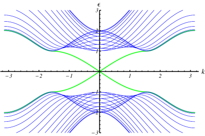
Figure 1: (Color online) Full band structure $\varepsilon(k)$ of a 2DTI with $\Delta=2B$, $A=B=1$ and $N=30$. The blue curves correspond to the bulk modes while the two green curves represent the topological surface states. Each state is doubly degenerate with respect to the two eigenvalues of the $\sigma_{x}$ matrix.

The calculated energy dispersion corresponding to Eq. (6) is presented in Fig. 1. For $0<\Delta/B<4$, two localized states at the boundaries are obtained, which may be expressed in terms of a linear combination of the ansatz wave functions Imura et al. (2010)

$$\Psi_{j,\,l}=\frac{1}{\sqrt{Na}}\sum\limits_{k}\,\psi^{>}_{j}(k)\,\texttt{e}^{ikl}+\frac{1}{\sqrt{Na}}\sum\limits_{k}\,\psi^{<}_{j}(k)\,\texttt{e}^{-ikl}$$ (7)

$$=\frac{1}{\sqrt{Na}}\sum\limits_{k}\,\left[\rho(k)\right]^{j}\,\texttt{e}^{ikl}+\frac{1}{\sqrt{Na}}\sum\limits_{k}\,\left[\rho(k)\right]^{N+1-j}\,\texttt{e}^{-ikl}\ ,$$

where the helical states are chosen to be the eigenstates defined by $\Gamma_{1}|{\pm}\rangle=\pm\,|{\pm}\rangle$. The analytic solutions of Eq. (7) may be obtained by substituting the above ansatz wave functions into Eq. (6) and considering the identity $\left[i\Gamma_{5}\Gamma_{2},\,\Gamma_{1}\right]=0$. This yields

$$\psi^{>}_{j}(k)=\left({c^{>}_{+,1}[\rho_{1}(k)]^{j}+c^{>}_{+,2}[\rho_{2}(k)]^{j}}\right)|{+}\rangle$$ (8)

$$+\left({c^{>}_{-,1}[\rho_{1}(k)]^{-j}+c^{>}_{-,2}[\rho_{2}(k)]^{-j}}\right)|{-}\rangle\ ,$$

$$\psi^{<}_{j}(k)=\left({c^{<}_{-,1}[\rho_{1}(-k)]^{N+1-j}+c^{<}_{-,2}[\rho_{2}(-k)]^{N+1-j}}\right)|{-}\rangle$$

$$+\left({c^{<}_{+,1}[\rho_{1}(-k)]^{-N-1+j}+c^{<}_{+,2}[\rho_{2}(-k)]^{-N-1+j}}\right)|{+}\rangle\ .$$

The wave function corresponding to $|{+}\rangle$ in Eq. (8) is related to the energy dispersion $E_{+}(k)=A\,\texttt{sin}(k)$, while that corresponding to $|{-}\rangle$ is associated with $E_{-}(k)=-A\,\texttt{sin}(k)$, as shown by two green curves in Fig. 1. The deviation from the sine function becomes significant once $E_{\pm}(k)$ merges with the bulk modes (shown as blue curves). Parameters $\rho_{1}(k)$ and $\rho_{2}(k)$ in Eq. (8) are defined by

$$\rho_{1,\,2}(k)=\frac{-\Omega(k)\pm\sqrt{\Omega^{2}(k)+A^{2}-4B^{2}}}{A+2B}\ ,$$ (9)

$$\Omega(k)=\Delta-2B\left[{2-\texttt{cos}(k)}\right]\ .$$ (10)

For $A=B=1$ and $k=0$, the variation of these parameters with respect to $\Delta/B$ is displayed in Fig. 2.

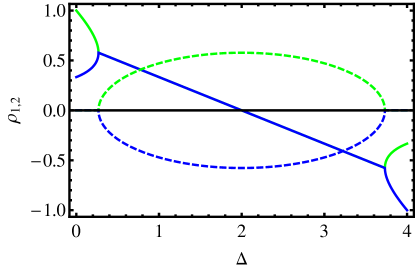
Figure 2: (Color online) Based on Eq. (10) the real (solid curves) and imaginary (dashed curves) parts of $\rho_{1}$ (green) and $\rho_{2}$ (blue) at $k=0$ as a function of $\Delta/B$ for $A=B=1$.

Since our interest is limited to calculating the plasmon dispersion in the long-wavelength limit, we would only consider the case with $k\ll 1$. This leads to the approximate expression $E_{\pm}(k)\approx\pm Ak$, and $\rho_{1,\,2}(k)\approx\rho_{1,\,2}(0)$ become $k$-independent at the same time. For $\Delta=2B$, we find $\rho_{1,\,2}=\pm i/\sqrt{3}$.

The coefficients $c_{\pm,\,\alpha}$ with $\alpha=1,\,2$ in Eq. (8) may be determined from the boundary conditions as well as the wave function normalization condition. By choosing $N\gg 1$, the condition for a finite-valued wave functions requires $c^{>}_{-,\,\alpha}=c^{<}_{+,\,\alpha}=0$. Moreover, the vanishing boundary conditions lead to $c^{>}_{+,\,1}+c^{>}_{+,\,2}=0$ and $c^{<}_{-,\,1}+c^{<}_{-,\,2}=0$. After normalizing the wave functions in Eq. (8), we find $c^{>}_{+,\,1}=c^{<}_{-,\,1}=2/\sqrt{3}$. Therefore, the two components of the wave function in Eq. (7) do not overlap and are localized on opposite boundaries. In addition, the eigenvalues of the spin state of $\sigma_{x}$ are related to the sign of the group velocity, i.e., $\psi^{>}_{j}$ corresponds to $E_{+}(k)$ while $\psi^{<}_{j}$ is related to $E_{-}(k)$. This pair of fermions constitutes a $1$-component HL, and is connected by the time-reversal symmetry. For a semi-infinite quantum well with $N\rightarrow\infty$ and $\rho_{1,\,2}=\pm i/\sqrt{3}$, on the other hand, we are left with a single helical state localized at the $j=0$ boundary

$$\psi^{>}_{j}\approx\frac{2(i)^{j}}{(\sqrt{3})^{j+1}}\left[{1-(-1)^{j}}\right]|{+}\rangle\ ,$$ (11)

$$E_{+}(k)\approx Ak\ .$$

If the material parameters $|{\rho_{1,\,2}}|>1$ are chosen, one would retain the left mover $\psi^{<}_{j}$ proportional to $|{-}\rangle$ as the proper solution. For a $2$-component HL (Kramers pair), we must consider two helical states on each edge. Those two states are related in Eq. (8) by the spin change $|+\rangle\leftrightarrow|-\rangle$ and the time reversal $k\leftrightarrow-k$ as well. Therefore, the second part of the Kramers pair is:

$$\psi^{>}_{j}\approx\frac{2(i)^{j}}{(\sqrt{3})^{j+1}}\left[{1-(-1)^{j}}\right]|{-}\rangle\ ,$$ (12)

$$E_{-}(k)\approx-Ak\ .$$

III Plasmons in HL compared with 1DEG

Based on the calculated full band structure from the BHZ model, we will further study the electron screening dynamics from the dielectric function of a 2DTI system. The edge states in such a system appear as the Kramers pair (Eq. (11)) with the electron spin attached to its momentum. On the level of density-density response it is imposable to break up the Kramers pair into its components, thus observing the response of the two component HL. However in the next section we shall show that the density-density response of the single component HL formally correspond to the interference pattern of the density-density and spin-density waves of the two component HL.

We shall formally start with the density-density response of the single component HL. Specifically, we will consider a semi-infinite type-III quantum well, in which only one helical state can occur and is localized around the edge ($y=0$) of the system. As a result, there exist only intraband transition in our system. For the wave function given by Eq. (11), the plasmon excitation dispersion $\omega_{p}(q)$ within the random-phase approximation (RPA) is determined by the zero of the following dielectric function

$$\epsilon(q,\,\omega)=1-V(q)\,\Pi_{+,+}(q,\,\omega+i0^{+})$$ (13)

$$=1-\frac{1}{\pi}\,\frac{qV(q)}{\hbar\omega-Aq}+iq\,V(q)\,\delta(\hbar\omega-Aq)\ ,$$

where the noninteracting polarization function at zero temperature is given by

$$\Pi_{+,+}(q,\,\omega+i0^{+})=\frac{1}{N}\sum\limits_{k}\,\frac{\theta(k+q)-\theta(k)}{E_{+}(k)-E_{+}(k+q)+\hbar\omega+i0^{+}}$$ (14)

$$=\frac{2}{2\pi}\,\frac{q}{\hbar\omega-Aq+i0^{+}}\ .$$

Here, $\theta(x)$ is the unit step function and $E_{F}=0$ is assumed for the Fermi energy. The perfector of two in Eq. (14) accounts for the double degeneracy of the bands. Very importantly, the time-reversal symmetry is broken in Eq. (14) for the response function, i.e., $\Pi_{+,+}(q,\,\omega+i0^{+})\neq\Pi^{\ast}_{+,+}(q,\,-\omega+i0^{+})$. The Coulomb matrix element introduced in Eq. (13) is given by Li and Das Sarma (1991)

$$V(q)=\frac{2e^{2}}{\epsilon_{s}a}\sum\limits_{j=1}^{\infty}\,\sum\limits_{j^{\prime}=j+1}^{\infty}\,|{\psi^{>}_{j}}|^{2}|{\psi^{>}_{j^{\prime}}}|^{2}\,K_{0}\left[{q(j^{\prime}-j)}\right]\ ,$$ (15)

where $K_{0}(x)$ is the modified Bessel function of the second kind, $\epsilon_{s}=\epsilon_{0}\epsilon_{b}$ and $\epsilon_{b}$ is the dielectric constant of the host material. If it is not explicitly stated, our parameters of choice are $A=B=1$ and $\Delta=2B$ in this paper. For this parameter choice, the summation in Eq. (15) can be carried out explicitly to give

$$V(q)=\frac{2e^{2}}{\epsilon_{s}a}\int\limits_{0}^{\infty}\,\frac{12\texttt{cos}(qt)\,dt}{5\sqrt{1+t^{2}}\left[{41-9\texttt{cos}(2qt)}\right]}$$ (16)

$$\approx\frac{e^{2}}{\epsilon_{s}a}\,\frac{3}{20}\,K_{0}(q)\ .$$

Here, the validity of the last approximation is demonstrated in Fig. 3, and the perfector can be calculated, by using the fine-structure constant and $\epsilon_{b}=7$ for HgTe, as $e^{2}k_{B}/\epsilon_{s}A=4\pi\times 0.001(\hbar k_{B}v_{F}/A)(c/v_{F})\approx 4\pi$.

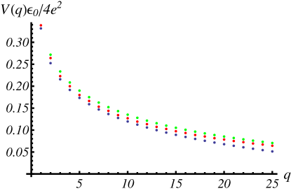
Figure 3: (Color online) The $q$ dependence (in units of the reciprocal inter-atomic spacing $a$) of the scaled Coulomb matrix element $V(q)/(4e^{2}/\epsilon_{s}a)$ in Eq. (15) evaluated between its upper $(3/40)\,K_{0}(q)$ (green) and lower bound $-(3/40)\,\ln(q)$ (black) for various values of the ratio $\Delta/B$, where $A=B=1$. The result for the approximate expression in Eq. (16) is given by red dots in the figure.

The imaginary part of the dielectric function in Eq. (13) yields the boundary $\hbar\omega_{p-h}=Aq$ for the particle-hole excitation region. Collapse of the particle-hole region into the single line is characteristic to the linear dispersion Brey and Fertig (2007). Zeros of the real part give rise to the plasmon dispersion relation:

$$\hbar\omega_{p}(q)=Aq\left[{1+\frac{1}{\pi A}\,V(q)}\right]\ .$$ (17)

In the long-wavelength limit with $qa\ll 1$, we obtain $\texttt{Re}[\Pi_{+,+}(q,\,\omega+i0^{+})]=q/\pi\hbar\omega+{\cal O}(q^{2})$ as a leading-order result. In conjunction with Eq. (16), the above equation leads to the explicit plasmon dispersion relation in the long-wavelength limit:

$$\omega_{p}(q)=-\omega_{0}\,q\ln(q)+{\cal O}(q^{3})\ ,$$ (18)

$$\hbar\omega_{0}=\frac{e^{2}}{\pi\epsilon_{s}a}\,\frac{3}{20}\ .$$

Results from our calculations based on Eqs. (16), (17) and (18) are presented in Fig. 4. It is found that $A=B=1$ and $\Delta=2B$ gives us the lower boundary of the plasmon excitation energy. This implies that the variations of $A$, $B$ and $\Delta$ within the regime in which the topological edge state exists results in an increase in the plasmon energy.

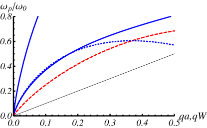
Figure 4: (Color online) Scaled plasmon excitation energy $\omega_{p}(q)/\omega_{0}$ of 2DTI (blue solid curve) given by Eq. (17) with $A=B=1$. The lower blue solid curve corresponds to $\Delta=2B$, while the upper blue solid curve is for $\Delta=B$ or $\Delta=3B$. The result of Eq. (18) is given by the dashed blue curve in the long-wavelength limit. The conventional 1DEG plasmon dispersion is indicated by a red dashed curve. The particle-hole excitation region is represented by a thin black straight line.

Most inelastic scattering experiments measure the dynamic structure factor $\sim\texttt{Im}[\epsilon^{-1}(q,\,\omega)]$ or the inverse dielectric function. We display $\texttt{Im}[\epsilon^{-1}(q,\,\omega)]$ in Fig. 5 as a function of $\omega$ for chosen values of $q$. Clearly, the spectrum of $\texttt{Im}[\epsilon^{-1}(q,\,\omega)]$ is dominated by the plasmon resonance. The particle-hole excitation is not pronounced in this figure. Around the plasmon resonances, we can employ the plasmon-pole approximation $\texttt{Im}[\epsilon^{-1}(q,\,\omega)]\sim\beta_{q}\,\delta(\omega-\omega_{p})$, where the plasmon weight is defined by

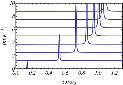
Figure 5: Spectral function $\texttt{Im}[\epsilon^{-1}(q,\,\omega)]$ of single component HL in 2DTI as a function of $\omega/\omega_{0}$ with and chosen $q$. Here, the curves with different values for $q$ are offset vertically for clarity.

$$\beta_{q}=\frac{\pi}{\left[{\partial\texttt{Re}\,\epsilon(q,\,\omega)/\partial\omega}\right]_{\omega=\omega_{p}}}$$ (19)

$$=-\frac{\pi^{2}\hbar\omega_{0}^{2}q\,\texttt{ln}^{2}(q)}{V(q)}\ .$$ (20)

Although varying the parameters of a 2DTI system from those producing the minimal $\omega_{p}(q)$ can increase the plasmon energy, it reduces the plasmon weight.

Now, let us compare our result with several known cases of 1DEG. For a conventional semiconductor quantum wire with a parabolic energy dispersion $E_{0}(k)=\hbar^{2}k^{2}/2m^{\ast}$ for conduction electrons, the intraband plasmon dispersion in the long-wavelength limit can be written as Zhu et al. (1989); Li and Das Sarma (1991); Sarma and Hwang (1996)

$$\omega_{p}(q)=\omega_{0}\,q\sqrt{-\ln(q)}+{\cal O}(q^{3})\ ,$$ (21)

$$\omega_{0}=\left({\frac{2v_{F}e^{2}}{\pi\hbar\epsilon_{s}W^{2}}}\right)^{1/2}=\left({\frac{2n_{1D}e^{2}}{\epsilon_{s}m^{\ast}W^{2}}}\right)^{1/2}\ ,$$

where $n_{1D}$ and $m^{\ast}$ denote the electron linear density and effective mass, respectively. For 1DEG, the wave vector $q$ is scaled with the characteristic size $W$ of the nanowire, i.e., $q\rightarrow qW$. The linear scaling of the plasmon frequency with the square-root of electron density as well as the high sensitivity to the wire characteristic size $\sim\sqrt{-\ln(qW)}$ are the unique properties of 1DEG in conventional semi-conducting nanowires. These properties are in sharp contrast with our result in Eq. (21) for localized quasi-1DEG in a 2DTI system.

For the conventional 1DEG, the plasmon weight is given by

$$\beta_{q}\sim\frac{q\left[{-\texttt{ln}(q)}\right]^{3/2}}{V_{c}(q)}\ ,$$ (22)

$$V_{c}(q)=\frac{2e^{2}}{\epsilon_{s}W}\left[{K_{0}(q)+1.972}\right]\ ,$$

which has different power dependence for the term $\sim\ln(q)$. Comparison of the plasmon weights are shown in Fig. 6 for both the TI-based and conventional 1DEG. From Fig. 6, we find that the plasmon weight in 2DTI is an order of magnitude larger than that of the conventional 1DEG. Consequently, a much more pronounced dynamical structure factor is expected for 2DTI [compare Fig. 5 here with Fig.  7 of Ref. Sarma and Hwang (1996)]. We also note that the particle-hole excitation spectrum exists in a wide region $k_{F}q/m^{\ast}-\hbar^{-1}E_{0}(q)<\omega_{p-h}<k_{F}q/m^{\ast}+\hbar^{-1}E_{0}(q)$ for a conventional 1DEG rather than a narrow line in 2DTI.

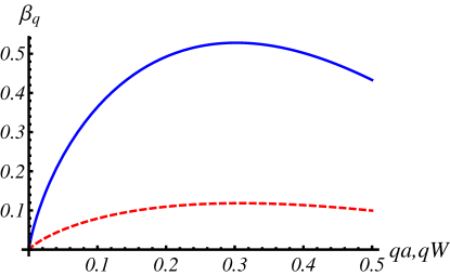
Figure 6: (Color online) Plasmon weight $\beta_{q}$ for TI-based (blue solid curve) and conventional (dashed red curve) 1DEGs, where $\omega_{0}$ is chosen as the same for both cases.

One of the striking features of 1DEG is that the RPA becomes exact for small value vectors $q$. This implies that the quasi-particles obtained from the exactly solvable linearized Tomonaga-Lüttinger model agree with the calculated plasmon dispersion relation in the RPA Li et al. (1992). In the case of a single-component HL for a 2DTI system, only one electron branch in the Tomonaga-Lüttinger model should be included.

It is also very interesting to compare the results in our paper with similar ones for graphene-based nanostructures, where 1DEG is provided by chiral-state electrons. A detailed calculation using RPA for plasmon excitations in both armchair and zigzag edged graphene-based nanoribbons was carried out by Brey and Fertig Brey and Fertig (2007), and only the armchair type was found to exhibit undamped plasmon excitations. The most interesting finding in Brey and Fertig’s work is the presence of metallic nanoribbons with the lowest electronic bands given by $E_{\pm}(k)=\pm\hbar v_{F}|{k}|$. In these metallic nanoribbons, the electron wave functions favor forward scattering. The scattering between the branches of different helicity is prohibited and corresponding structure factor vanishes. Both helical branches (given value of the pseudo-spin) contribute equally to the response . As a result, the polarization retains time-reversal symmetry. For metallic graphene nanoribbons, we obtain the interband polarization function

$$\chi_{1}(q,\,\omega+i0^{+})=\Pi_{+,-}(q,\,\omega+i0^{+})+\Pi_{-,+}(q,\omega+i0^{+})$$ (23)

$$=\frac{1}{\pi}\left[\frac{q}{\hbar\omega-\hbar v_{F}q+i0^{+}}-\frac{q}{\hbar\omega+\hbar v_{F}q+i0^{+}}\right]$$

$$=\frac{2}{\pi}\,\frac{\hbar v_{F}q^{2}}{\left({\hbar\omega+i0^{+}}\right)^{2}-(\hbar v_{F}q)^{2}}\ .$$

Note that the polarization subindex here is related to the valley index rather than to the pseudo-spin. At the same time, the intraband polarization functions, $\Pi_{-,-}(q,\,\omega+i0^{+})$ and $\Pi_{+,+}(q,\omega+i0^{+})$, vanish due to time-reversal symmetry. This, in turn, results in the plasmon dispersion in Eq. (21) with electron Fermi velocity independent of the electron density. In other words, we have $v_{F}=\texttt{const}$ as in the case of 2DTI. Except for the spin factor of $2$, the polarization function in Eq. (23) is identical to the two-component HL in 2DTI (i.e., both electron spin states are excited). From Eqs. (18), (21) and Fig. 4, one can easily understand that the energies of the collective excitations for the two and single component HLs are well separated in spectrum, but they share the same particle-hole excitation region.

For graphene, the plasmon excitations in doped semiconductor armchair nanoribbons are similar to the conventional 1DEG plasmon dispersion. The localization of electron wave functions along two ribbon edges can be obtained in zigzag nanoribbons. However, the cone-like band structure disappears for this case. Moreover, the particle-hole excitations cover a broad region, instead of a narrow line, and the plasmon dispersion which falls into this broad region becomes Landau damped.

IV Single component HL response as a spin-density wave.

The above paragraph was arguing on strong plasmon branch separation in single and two component electron HL. However, single component HL is somehow an artificial concept since the topological states always appear as Kramers pair. Below we shall demonstrate that the density-density plasmon excitations of single component HL are actually equivalent to the spin-density plasmons in two component HL. As a by-product, we shall also consider spin-spin waves and compare them to those in a conventional 2DEG.

Now let us provide theoretical description of the spin-spin and spin-density waves. For that purpose, we shall need the inter-spin polarizations ($\Pi_{\pm,\mp}$) as well as intra-spin polarizations ($\Pi_{\pm,\pm}$). The intra-spin polarizations are given in Eq. (23). The interspin polarizations are also connected by $\Pi_{+,-}(q,\omega)=\Pi_{-,+}(q,\omega)$. Here,

$$\Pi_{-,+}(q,\omega)=\int\limits_{-k_{c}}^{k_{c}}dk\frac{\theta(E_{-}(k+q))-\theta(E_{+}(k))}{E_{+}(k)-E_{-}(k+q)+\omega}$$ (24)

$$=-\frac{1}{2A}\left[{\texttt{Log}\left({2Ak_{c}+Aq+\omega}\right)+\texttt{Log}\left({-2Ak_{c}+Aq+\omega}\right)}\right]\ ,$$

where we have introduced a cut-off wave vector $k_{c}>q$ due to logarithmic divergence of the above integral when the chemical potential is set to zero. In the long wave approximation $(Aq+\omega)/2Ak_{c}\ll 1$, we can simplify the inter-spin polarization as:

$$\Pi_{-,+}(q,\omega)$$ (25)

$$=-\frac{1}{2A}\left[{i\pi+\texttt{Log}\left({2Ak_{c}}\right)-\frac{1}{4A^{2}k^{2}_{c}}\left({\omega+Aq}\right)^{2}}\right]\ .$$

Therefore, two-component helical liquid (Kramers pair) obeys the same response function as multi-level electron plasma Kushwaha et al. (2006). The generalized nonlocal, dynamic dielectric-function matrix connects external $\hat{V}_{ext}$ and induced $\hat{V}_{ind}$ perturbation potential matrix elements:

$$\langle{\nu}|{V_{ext}}|{\nu^{\prime}}\rangle=\sum\limits_{\mu,\mu^{\prime}}\epsilon^{\rho,\rho}_{\mu\mu^{\prime};\nu\nu^{\prime}}\langle{\mu}|{V_{ind}}|{\mu^{\prime}}\rangle\ ,$$ (26)

$$\epsilon^{\rho,\rho}_{\mu\mu^{\prime};\nu\nu^{\prime}}=\delta_{\mu,\nu^{\prime}}\delta_{\mu^{\prime},\nu}-V_{q}S^{\rho,\rho}_{\mu\mu^{\prime};\nu\nu^{\prime}}\Pi_{\mu,\mu^{\prime}}(q,\omega)\ .$$ (27)

Here, the superscript $\rho,\rho$ indicates density-density response; $V_{q}=V(q)$ in Eq. (15); the sates $|{\mu}\rangle=|{\pm}\rangle$ indicate the spin component of the Kramers pair (eigenfunctions of $\hat{\sigma}_{z}$ Pauli matrix). The spin overlap function is given by:

$$S^{\rho,\rho}_{\mu\mu^{\prime};\nu\nu^{\prime}}=\langle{\mu}|\sigma_{0}|{\mu^{\prime}}\rangle\langle{\nu}|{\sigma_{0}}|{\nu^{\prime}}\rangle$$ (28)

with $\sigma_{0}$ being an identity operator. Explicitly, Eq. (27) can be written as:

$$\epsilon^{\rho,\rho}=\left({\begin{matrix}1-V_{q}\Pi_{+,+}&0&0&-V_{q}\Pi_{+,+}\\ 0&1&0&0\\ 0&0&1&0\\ -V_{q}\Pi_{-,-}&0&0&1-V_{q}\Pi_{-,-}\end{matrix}}\right)\ ,$$ (29)

whose inverse is:

$$\left({\epsilon^{\rho,\rho}}\right)^{-1}\sim\frac{1}{1-V_{q}\left({\Pi_{+,+}+\Pi_{-,-}}\right)}\ .$$ (30)

In order to consider spin-spin response, we shall introduce the spin-lowering $\hat{\sigma}_{\downarrow}$ and spin-raising $\hat{\sigma}_{\uparrow}$ operators by their action on the spin states:

$$\begin{matrix}\sigma_{\downarrow}|{+}\rangle=|{-}\rangle;&\sigma_{\downarrow}|{-}\rangle=|{0}\rangle\ ,\\ \sigma_{\uparrow}|{+}\rangle=|{0}\rangle;&\sigma_{\uparrow}|{-}\rangle=|{+}\rangle\ ,\end{matrix}$$

$$\langle{0}|{\pm}\rangle=0\ .$$

The spin-spin generalized functions are given by Eq. (27) with

$$S^{\uparrow,\downarrow}_{\mu\mu^{\prime};\nu\nu^{\prime}}=\langle{\mu}|\sigma_{\uparrow}|{\mu^{\prime}}\rangle\langle{\nu}|{\sigma_{\downarrow}}|{\nu^{\prime}}\rangle\ ,$$ (31)

$$S^{\downarrow,\uparrow}_{\mu\mu^{\prime};\nu\nu^{\prime}}=\langle{\mu}|\sigma_{\downarrow}|{\mu^{\prime}}\rangle\langle{\nu}|{\sigma_{\uparrow}}|{\nu^{\prime}}\rangle\ .$$

The explicit form of the dielectric function is:

$$\epsilon^{\uparrow,\downarrow}=\texttt{diag}\left[{1,1-V_{q}\Pi_{+,-},1,1}\right]\ ,$$ (32)

$$\epsilon^{\uparrow,\downarrow}=\texttt{diag}\left[{1,1,1-V_{q}\Pi_{-,+},1}\right]\ ,$$

and the spin-spin waves are given by real zeros of :

$$\left({\epsilon^{\uparrow,\downarrow}+\epsilon^{\downarrow,\uparrow}}\right)^{-1}\sim\frac{1}{1-V_{q}\left({\Pi_{+,-}+\Pi_{-,+}}\right)}\ .$$ (33)

Dispersion curves of the spin-spin waves are shown in Fig. 7

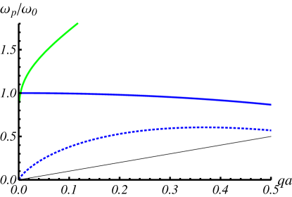
Figure 7: Spin-Spin wave (Eq. (35)) and the plasmons (Eq. (30)) in TI. Thick blue curve correspond to spin-wave with large critical cut-off $1/(2A)V_{q}\texttt{Log}(2Ak_{c})\gg 1$. Thick green curve is the spin-wave with the cut-off in the linear regime of the dispersion $2Ak_{c}=1$. Dotted curve is the plasmon mode while thin black line is the particle-hole excitations.

Note that in the limit of large cut-off wave vector $1/(2A)V_{q}\texttt{Log}(2Ak_{c})\gg 1$, the spin-wave is analogues to $\Omega_{-}$ inter-spin branch in case of Rashba spin-orbit Kushwaha et al. (2006). The plasmon branch is similar to $\Omega_{0}$ of intra-spin plasmon. $\Omega_{-}$ inter-spin branch has no analogue in TI case. The reason to that is four possible inter-spin transitions in the Rashba split 2DEG as opposite to two of those in TI.

The spin-density response is defined by Lozovik Efimkin et al. (2011) as Eq. (27) with the spin overlap given by:

$$S^{\rho,\bar{\sigma}}_{\mu\mu^{\prime};\nu\nu^{\prime}}=\langle{\mu}|\sigma_{0}|{\mu^{\prime}}\rangle\langle{\nu}|{\bar{\sigma}}|{\nu^{\prime}}\rangle\ ,$$ (34)

where $\bar{\sigma}=\left[{\sigma_{x}=\sigma{\uparrow}+\sigma{\downarrow},\sigma_{y}=-i\left({\sigma{\uparrow}-\sigma{\downarrow}}\right),\sigma_{z}}\right]$. One can show that

$$\epsilon^{z,z}=\epsilon^{\rho,\rho}\ ,$$ (35)

$$(\epsilon^{x,x})^{-1}\sim\frac{1}{1-V_{q}\left({\Pi_{+,-}+\Pi_{-,+}}\right)}\ ,$$

$$(\epsilon^{y,y})^{-1}\sim\frac{1}{1-V_{q}\left({\Pi_{+,-}+\Pi_{-,+}}\right)}\ .$$

Due to the fact that in 3DTI the spin wave function component depends on wave vector, we are left with only transverse $\langle\sigma^{z}\rangle$ component of the response survive. In our case, those actually provide the spin-spin waves. Those spins may be coupled to the density via $\epsilon^{\rho,x},\epsilon^{\rho,y}$. However, the inverse of those matrices does not provide any resonances, and then, such coupling may be neglected. On the other hand, we find the rest inverse as:

$$(\epsilon^{\rho,z})^{-1}\sim\frac{1}{1-V_{q}\left({\Pi_{-,-}-\Pi_{+,+}}\right)}\ ,$$ (36)

$$(\epsilon^{\rho,-z})^{-1}\sim\frac{1}{1-V_{q}\left({\Pi_{+,+}-\Pi_{-,-}}\right)}\ .$$ (37)

In the above two equations, the time reversal symmetry is broken, similar (but not identical) to the case of single component HL discussed in the previous section. There are four spin-plasmon modes:

$$\pi\omega_{p}^{\rho,\pm z}=\mp qv_{q}\pm\sqrt{(\pi Aq)^{2}+(qV_{q})^{2}}\ .$$ (38)

Apart from a factor of two, in the long wave approximation we shall obtain the mode given by the single component HL:

$$\omega^{\rho,-z}_{p}=\frac{2}{\pi}qV_{q}=-2\omega_{0}q\texttt{ln}(q)\ .$$ (40)

Due to Eq. (35) the combined spin-density response can be written via the spin-density overlap as:

$$S^{\rho,\rho\pm\sigma_{z}}_{\mu\mu^{\prime};\nu\nu^{\prime}}=\langle{\mu}|\sigma_{0}|{\mu^{\prime}}\rangle\langle{\nu}|{\sigma_{0}\pm\sigma_{z}}|{\nu^{\prime}}\rangle\ ,$$ (41)

so that we recover the single-component HL response:

$$(\epsilon^{\rho,\rho\pm z})^{-1}\sim\frac{1}{1-V_{q}\Pi_{\mp,\mp}}\ .$$ (42)

To conclude this paragraph we have demonstrated that the spin-density response mimics that of single component helical liquid. Also we found similar behavior of spin-spin waves in TI to those provided by Rashba spin-orbit split in a conventional 2DEG.

V Concluding Remarks

The dispersion of intraband plasmon excitations in a semi-infinite inverted HgTe/CdTe quantum well has been derived within the random-phase approximation based on a calculated edge-localized topological state of electrons in a single-component helical liquid using the BHZ model. Under the perturbation from a linearly-polarized incident light, the unique properties in the collective excitation of these edge-bound electrons with a broken time-reversal symmetry has been explored. Our calculations predict the plasmon dispersion $\omega_{p}(q)\sim-\omega_{0}q\,\texttt{ln}(qa)$ for such a single-component helical state in the long-wavelength limit, in sharp contrast with $\omega_{p}(q)\sim-\omega_{0}\sqrt{-\texttt{ln}(qW)}$ found for a one-dimensional electron gas in a quantum-wire system. Moreover, $\omega_{0}$ in our plasmon dispersion is independent of the linear electron density, similar to the case for a metallic armchair graphene nanoribbon. On the other hand, the plasmon dispersion of the two-component helical liquid is found to be identical to that of a armchair graphene nanoribbon except for the spin perfector and a characteristic-width scaling of the wave number. The particle-hole excitation region shrinks into a straight line in our system, in comparison with a wide region for a conventional one-dimensional electron gas. The plasmon energy of the single-component helical state is well separated from that of the two-component helical state but they share the common particle-hole excitation region in the excitation spectrum. The density-density plasmon excitations of single component HL are equivalent to the spin-density plasmons in two component HL.