Mixed Beta Regression: A Bayesian Perspective

Abstract

This paper builds on recent research that focuses on regression modeling of continuous bounded data, such as proportions measured on a continuous scale. Specifically, it deals with beta regression models with mixed effects from a Bayesian approach. We use a suitable parameterization of the beta law in terms of its mean and a precision parameter, and allow both parameters to be modeled through regression structures that may involve fixed and random effects. Specification of prior distributions is discussed, computational implementation via Gibbs sampling is provided, and illustrative examples are presented.

1 Introduction

Mixed-effects models have been widely employed in statistical analysis, main-ly in the area of health, and their study has been primarily restricted to response variables with normal or, at least, symmetrical distributions. Such models are not appropriately applicable when the response variable has a support restricted to a doubly bounded interval. Limited-range variables are, however, common in practice; for example, proportions are bounded between zero and one. This paper proposes a Bayesian analysis for mixed-effects regression models that are tailored for situations where the response variable is measured on a continuous scale and is restricted to the unit interval $(0,1)$. Situations where the response, say $y$, is limited to a known interval $(a,b)$ is also accommodated through the transformation $y^{*}=(y-a)/(b-a)$. The response variable is assumed to be beta distributed with mean (and possibly a precision parameter) modeled using fixed and random effects. The substantial advantage to consider a beta modeling is due to the flexibility that it provides. In fact, the beta family includes left or right skewed, symmetric, J-shaped, and inverted J-shaped distributions.

Following Ferrari and Cribari-Neto (2004), our proposed model uses a parameterization of the beta law in terms of its mean and an additional positive parameter that can be regarded as a precision parameter. The mean of the response variable is conveniently linked with a mixed-effects regression structure by the logit link function. An extended version of such a model is also considered. It assumes that the precision parameter is not constant over the observations, but rather it is related to a mixed-effects function through a log link.

To formulate our proposed models, we adopt a Bayesian approach. We address the issues of model fitting via Gibbs sampling, choice of prior distributions, and model selection based on the deviance information criterion, the expected Akaike information criterion and the expected Bayesian information criterion. Simulated and real data analysis are presented for illustration. An appendix presents various pieces of BUGS code used for fitting the mixed beta regression.

2 Bayesian mixed beta regression

Due to the flexibility of the beta distribution in terms of the variety of density shapes that can be accommodated, this distribution is a natural choice for modeling continuous data that are restricted to the interval $(0,1)$. The probability density function of a variable $y$ following a beta distribution parameterized in terms of its mean $\mu$ ($0<\mu<1$) and a precision parameter $\phi$ ($\phi>0$) is given by

$$f(y|\mu,\phi)=\frac{\Gamma(\phi)}{\Gamma(\mu\phi)\Gamma((1-\mu)\phi)}y^{\mu\phi-1}(1-y)^{(1-\mu)\phi-1},~{}~{}~{}~{}~{}0<y<1,$$ (1)

where $\Gamma(\cdot)$ denotes the gamma function. Note that $\phi$ can be interpreted as a precision parameter, since $\mu={\rm E}(y)$ and ${\rm Var}(y)=\mu(1-\mu)/(1+\phi)$ and, hence, for each fixed value of the mean $\mu$, $1+\phi$ is inversely proportional to the variance of $y$. If $y$ has density function (1), we write $y\sim{\rm beta}(\mu\phi,(1-\mu)\phi)$.

Now, let $y_{1},\ldots,y_{n}$ be $n$ independent random variables such that
$y_{i}\sim{\rm beta}(\mu\phi,(1-\mu)\phi)$. The definition of a beta regression model requires a transformation of the mean $\mu_{i}$ of $y_{i}$, $i=1,\ldots,n$, that maps the interval $(0,1)$ onto the real line. A convenient and popular link function is the logit link. It is then assumed that $\ln\{\mu_{i}/(1-\mu_{i})\}=x_{i}^{\top}\beta,$ where $x_{i}$ is a vector of known covariates for the $i$-th subject and $\beta$ denotes a vector of regression coefficients. The first element of $x_{i}$ is usually taken as 1 to allow for an intercept.

The precision parameter $\phi$ may be assumed to be constant over observations (Ferrari and Cribari-Neto, 2004) or it may be modeled in terms of a regression structure (Smithson and Verkuilen, 2006). Since the precision parameter is strictly positive, the log link function is a natural choice. It is then assumed that $\ln(\phi_{i})=w_{i}^{\top}\delta$ where $w_{i}$ is a vector of covariates and $\delta$ denotes a vector of unknown regression coefficients. Again, it is convenient to take the first element of $w_{i}$ as 1 to allow for an intercept in the precision description. There is no restriction on whether or not the $w_{i}$s contain the same predictor variables as $x_{i}$s.

The beta regression model described above does not involve random effects. Extending previous works on Bayesian generalized linear models (Dey et al., 2000) and Bayesian beta regression (Branscum et al., 2007), we define below two mixed beta regression models, the first of which assumes that the precision parameter is the same for all the observations, and the second involves a mixed-effects model for the precision parameter.

Let $y_{1},\ldots,y_{m}$ be independent continuous random vectors, where
$y_{i}=(y_{i1},\ldots,y_{in_{i}})^{\top}$ represents an observed response vector for a sample unit $i$ and for which each of its components, $y_{ij}$, takes values on the interval $(0,1)$. Consider also a regression model with the following structure:

$$G({\rm E}(y_{i}|b_{i}))=X_{i}\beta+Z_{i}b_{i},$$ (2)

$i=1,\ldots,m$, where $G(\cdot)$ is a vector-function linking the conditional mean response vector ${\rm E}(y_{i}|b_{i})$ with the linear mixed model $\eta_{i}=X_{i}\beta+Z_{i}b_{i}$, for which $X_{i}$ is the design matrix of dimension $n_{i}\times p$ corresponding to the vector $\beta=(\beta_{1},\ldots,\beta_{p})^{\top}$ of regression coefficients (the fixed effects) and $Z_{i}$ is the design matrix of dimension $n_{i}\times q$ associated with the vector $b_{i}=(b_{i1},\ldots,b_{iq})^{\top}$ (the random effects).

For the logit link function, the $j$-th component of (2) is

$$\ln\left\{\frac{\mu_{ij}}{1-\mu_{ij}}\right\}=\eta_{ij}=x_{ij}^{\top}\beta+z_{ij}^{\top}b_{i},$$

where $\mu_{ij}={\rm E}(y_{ij}|b_{i})$, $x_{ij}=(x_{ij1},\ldots,x_{ijp})^{\top}$, and $z_{ij}=(z_{ij1},\ldots,z_{ijq})^{\top}$, which is equivalent to

$$\mu_{ij}=\frac{\exp(\eta_{ij})}{1+\exp(\eta_{ij})}=\frac{\exp(x_{ij}^{\top}\beta+z_{ij}^{\top}b_{i})}{1+\exp(x_{ij}^{\top}\beta+z_{ij}^{\top}b_{i})}.$$ (3)

In this work, we first assume that for $i=1,2,\ldots,m$ and $j=1,2,\ldots,n_{i}$

$$y_{ij}|b_{i},\beta,\phi\stackrel{{\scriptstyle ind.}}{{\sim}}{\rm beta}(\mu_{ij}\phi,(1-\mu_{ij})\phi),$$

i.e., conditionally on $b_{i}$, $\beta$, and $\phi$, the $y_{ij}$’s are independent and have probability density function given by (1), with $\mu$ replaced by $\mu_{ij}$, which is specified by (3). Note that in this formulation, $\phi$ represents a common precision parameter.

In mixed models, the random effects $b_{1},\ldots,b_{m}$ are typically assumed to be independent and normally distributed, namely $b_{i}|{\Sigma_{b}}{\stackrel{{\scriptstyle ind.}}{{\sim}}}N_{q}(0,\Sigma_{b})$, $i=1,\ldots,m$, where $\Sigma_{b}$ is a positive-definite matrix. The normality assumption, however, can be inappropriate in practical applications where the measurements present outliers. In these cases, it is more adequate to consider multivariate distributions with heavier-than-normal tails for the random effects. Consequently, a multivariate $t$-distribution with $\nu_{b}>0$ degrees of freedom, location vector $\mu_{b}=0\in\mathbb{R}^{q}$ and positive-definite dispersion matrix $\Sigma_{b}$ is a better candidate to model the random effects $b_{i}$’s, i.e., $b_{i}|\nu_{b},{\Sigma_{b}}{\stackrel{{\scriptstyle ind.}}{{\sim}}}t_{q}(\nu_{b},0,\Sigma_{b})$, $i=1,\ldots,m$. It should be noticed here that for large values of $\nu_{b}$ the multivariate $t$-distribution is approximately a multivariate normal distribution.

In the mixed beta regression model proposed above, the precision parameter $\phi$ is constant over the observations. For a more general formulation of this model, we consider a different precision parameter, say $\phi_{ij}$, for each response $y_{ij}$. We then assume a mixed linear model for the logarithm of $\phi_{ij}$, namely

$$\ln(\phi_{ij})=\tau_{ij}=w_{ij}^{\top}\delta+h_{ij}^{\top}d_{i},$$ (4)

where $w_{ij}^{\top}=(w_{ij1},\ldots,w_{ijp^{*}})$ is the design vector corresponding to the $p^{*}\times 1$ vector $\delta$ of fixed effects and $h_{ij}^{\top}=(h_{ij1},\ldots,h_{ijq^{*}})$ is the design vector corresponding to the $q^{*}\times 1$ vector $d_{i}$ of random effects. Note that the design matrices $W_{i}=(w_{i1},\ldots,w_{in_{i}})^{\top}$ and $H_{i}=(h_{i1},\ldots,h_{in_{i}})^{\top}$ may, but are not required to, contain the same predictor variables as the matrices $X_{i}=(x_{i1},\ldots,x_{in_{i}})^{\top}$ and $Z_{i}=(z_{i1},\ldots,z_{in_{i}})^{\top}$, respectively. Here, it may be assumed that $d_{i}|{\Sigma_{d}}{\stackrel{{\scriptstyle ind.}}{{\sim}}}N_{q}(0,\Sigma_{d})$, $i=1,\ldots,m$, where $\Sigma_{d}$ is a positive-definite matrix. Alternatively, we may assume that $d_{i}|\nu_{d},{\Sigma_{d}}{\stackrel{{\scriptstyle ind.}}{{\sim}}}t_{q}(\nu_{d},0,\Sigma_{d})$, $i=1,\ldots,m$.

In order to complete the Bayesian specification of the beta mixed models described above, elicitation of prior distributions for all unknown parameters is required. Multivariate normal prior distributions are typically considered for the fixed effects, i.e., $\beta\sim N_{p}(\mu_{\beta},\Sigma_{\beta})$. Vague priors are usually specified by taking large values for the prior variances. However, the impact of the scale choice under the normal model cannot be neglected. An alternative strategy is to consider a multivariate $t$-distribution, i.e., $\beta\sim t_{p}(\nu_{\beta},\mu_{\beta},\Sigma_{\beta})$ and to specify an appropriated value for $\nu_{\beta}$, the degrees of freedom parameter. If the vector of random effects is assumed to follow a multivariate $t$-distributed, i.e., $b_{i}|\nu_{b},\mu_{b},\Sigma_{b}\sim t_{q}(\nu_{b},0,\Sigma_{b})$, then the prior distribution for the degrees of freedom can be discrete as in Albert and Chib (1993) and Besag et al. (1995), or continuous as in Geweke (1993). We have chosen the latter alternative. More specifically, we consider an exponential prior distribution with mean $1/a$ for the degrees of freedom, say $\varepsilon(a)$. The prior distribution for the scale matrix of random effects $\Sigma_{b}$ is chosen, mainly for computational simplicity, to be an inverted Wishart distribution as in Fong et al. (2010), i.e., $\Sigma_{b}\sim IW_{q}(\psi,c)$. An alternative prior distribution for $\Sigma_{b}$ is a constrained Wishart distribution (Everson and Morris, 2000).

We now turn to the specification of prior distributions for the precision parameter. As mentioned above, in this paper we study the following beta mixed regression models.

Model 1: It considers the mixed regression model (3) for the location parameters $\mu_{ij}$ and a common precision parameter $\phi$ for each observation $y_{ij}$. In the Bayesian context, a natural choice for the prior distribution of the precision parameter would be an inverse gamma distribution. If a slightly informative prior is required, it can be assumed that $\phi\sim IG(\epsilon,\epsilon)$, with a small fixed positive value for $\epsilon$. Gelman (2006) suggests that the prior distribution $\phi=\texttt{U}^{2}$ with $\texttt{U}\sim U(0,a)$ with large $a$ ($a=50$ for example) is less informative than an inverse gamma prior. Here, we propose a more flexible prior distribution for $\phi$ that includes Gelman’s prior distribution as a special case. More specifically, we propose the following prior specification for $\phi$: $\phi=(aB)^{2}$, where $B\sim{\rm beta}(1+\epsilon,1+\epsilon)$, for given positive values for $a$ and $\epsilon$.

Model 2: It considers the mixed regression model (3) for the location parameter $\mu_{ij}$ and a different precision parameter $\phi_{ij}$ for each $y_{ij}$, where $\phi_{ij}$ is modeled as in (4). Here, the specification of prior distributions for $\delta$ and the parameters of the distribution of the $d_{i}$s is similar to that used for $\beta$ and the parameters of the distribution of the $b_{i}$s.

3 Model fitting using Markov chain Monte Carlo sampling

Let $y^{\top}=(y_{1}^{\top},\ldots,y_{m}^{\top})$ and $\eta^{\top}=(\eta_{1}^{\top},\ldots,\eta_{m}^{\top})$, where $\eta_{i}^{\top}=(\eta_{i1},\ldots,\eta_{in_{i}})$. Note that, by assumption, conditionally on $\beta$, $\Sigma_{b}$, and $\nu_{b}$, the $\eta_{i}$s are independent and have density function $f(\eta_{i}|\beta,\Sigma_{b},\nu_{b})\propto f(b_{i}|\beta,\Sigma_{b},\nu_{b})$, $i=1,\ldots,m$. We now present the following results for the joint posterior distribution under models 1 and 2 described in the previous section.

Under model 1, and the assumption that the parameters $\Sigma_{b}$, $\nu_{b}$, $\phi$, and $\beta$ are independent, the joint posterior density is

$$f(\beta,\Sigma_{b},\nu_{b},\phi,\eta|y) \propto \left[\prod_{i=1}^{m}\prod_{j=1}^{n_{i}}f(y_{ij}|\eta_{ij},\phi)\right]$$

$$\times \left[\prod_{i=1}^{m}f(\eta_{i}|\beta,\Sigma_{b},\nu_{b})\right]f(\Sigma_{b})f(\nu_{b})f(\phi)f(\beta).$$

Gibbs sampling can be used to generate a Monte Carlo sample from the joint posterior density, $f(\beta,\Sigma_{b},\nu_{b},\phi,\eta|y)$. The Gibbs sampler in this context involves iteratively sampling from the full conditional distributions:

$$f(\Sigma_{b}|\nu_{b},\beta,\phi,\eta,y),\ \ \ f(\nu_{b}|\Sigma_{b},\beta,\phi,\eta,y),\ \ \ f(\beta|\Sigma_{b},\nu_{b},\phi,\eta,y),$$

$$f(\phi|\beta,\Sigma_{b},\nu_{b},\eta,y),\ \ {\rm and}\ \ f(\eta_{i}|\eta_{k},\beta,\Sigma_{b},\nu_{b},\phi,y_{i}),\ \ i,\,k=1,\ldots,m,\ \ i\neq k,$$

which can be implemented in the WinBUGS software. Posterior inferences on $\beta$, $\Sigma_{b}$, and $\phi$ and, more importantly, on the mean responses $(\mu_{ij};i=1,\dots,m,j=1,\ldots,n_{i})$ are readily obtained in WinBUGS. Hypothesis testing regarding regression coefficients and mean responses are also straightforward.

We now turn to model 2. Let $\tau^{\top}=(\tau_{1}^{\top},\ldots,\tau_{m}^{\top})$, where $\tau_{i}^{\top}=(\tau_{i1},\ldots,\tau_{in_{i}})$. By assumption, conditionally on $\delta$, $\Sigma_{d}$, and $\nu_{d}$, the $\tau_{i}$s are independent and have density function $f(\tau_{i}|\delta,\Sigma_{d},\nu_{d})\propto f(d_{i}|\delta,\Sigma_{d},\nu_{d})$, $i=1,\ldots,m$. Assuming prior independence of $\Sigma_{b}$, $\nu_{b}$, $\Sigma_{d}$, $\nu_{d}$, $\delta$, and $\beta$, we obtain the posterior density given by

$$f(\beta,\Sigma_{b},\nu_{b},\delta,\Sigma_{d},\nu_{d},\eta,\tau|y) \propto \left[\prod_{i=1}^{m}\prod_{j=1}^{n_{i}}f(y_{ij}|\eta_{ij},\tau_{ij})\right]$$

$$\times \left[\prod_{i=1}^{m}f(\eta_{i}|\beta,\Sigma_{b},\nu_{b})\right]\left[\prod_{i=1}^{m}f(\tau_{i}|\delta,\Sigma_{d},\nu_{d})\right]$$

$$\times f(\Sigma_{b})f(\nu_{b})f(\delta)f(\Sigma_{d})f(\nu_{d})f(\beta).$$

Similarly to model 1, the Gibbs sampling can be used to generate a Monte Carlo sample from $f(\beta,\Sigma_{b},\nu_{b},\delta,\Sigma_{d},\nu_{d},\eta,\tau|y)$. In this case, the Gibbs sampler involves iteratively sampling from the following full conditional distributions:

$$f(\Sigma_{b}|\nu_{b},\beta,\delta,\Sigma_{d},\nu_{d},\eta,\tau,y),\ \ \ f(\nu_{b}|\Sigma_{b},\beta,\delta,\Sigma_{d},\nu_{d},\eta,\tau,y),$$

$$f(\beta|\Sigma_{b},\nu_{b},\delta,\Sigma_{d},\nu_{d},\eta,\tau,y),\ \ \ f(\delta|\beta,\Sigma_{b},\nu_{b},\Sigma_{d},\nu_{d},\eta,\tau,y),$$

$$f(\Sigma_{d}|\beta,\Sigma_{b},\nu_{b},\delta,\nu_{d},\eta,\tau,y),\ \ \ f(\nu_{d}|\beta,\Sigma_{b},\nu_{b},\delta,\Sigma_{d},\eta,\tau,y),$$

$$f(\eta_{i}|\eta_{k},\tau_{k},\beta,\Sigma_{b},\nu_{b},\delta,\Sigma_{d},\nu_{d},y_{i}),\ \ {\rm and}\ \ f(\tau_{i}|\tau_{k},\eta_{k},\beta,\Sigma_{b},\nu_{b},\delta,\Sigma_{d},\nu_{d},y_{i}),$$

for $i,\,k=1,\ldots,m,$ and $i\neq k,$ which can be also implemented in the WinBUGS software. Thus, posterior inferences on $\beta$, $\Sigma_{b}$, and $\phi_{ij}$, for $i=1,\dots,m,$ $j=1,\ldots,n_{i}$, and on the mean responses $\mu_{ij}$, for $i=1,\dots,m,$ $j=1,\ldots,n_{i}$ are easily obtained in WinBUGS. Again, hypothesis testing regarding regression coefficients and mean responses are also straightforward.

4 Illustration via simulations

${}^{{}^{{}^{.}}}$
To illustrate the proposed methodology, we consider the following mixed beta regression model with simulated data (model 1):

$$y_{ij}|b_{i},\phi,\beta \sim {\rm beta}(\mu_{ij}\phi,(1-\mu_{ij})\phi),$$

where $\beta=(\beta_{1},\beta_{2},\beta_{3})^{\top}$, $b_{i}=(b_{i1},b_{i2})^{\top}$,

$$\ln\left\{\frac{\mu_{ij}}{1-\mu_{ij}}\right\}=\eta_{ij}=(\beta_{1}+b_{i1})+(\beta_{2}+b_{i2})x_{ij2}+\beta_{3}x_{ij3},$$

$i=1,\ldots,100$, $j=1,\ldots,5$, and $b_{i}|\nu_{b},\!\Sigma_{b}\sim t_{2}(\nu_{b},0,\Sigma_{b}).$ For our simulation study, the values of the covariates were generated from a uniform distribution in the unit interval, and we set $\nu_{b}=10$, $\phi=49$, $\beta=(-2,1,2)^{\top}$, and

$$\Sigma_{b} = \left(\begin{array}[]{rr}1&~{}-0.3\\ -0.3&~{}0.2\\ \end{array}\right).$$

As proposed in Section 2, we adopt the following prior specifications: $\nu_{b}\sim\varepsilon(a)$, $\Sigma_{b}\sim IW_{2}(\Psi,c)$, and $\beta=(\beta_{1},\beta_{2},\beta_{3})^{\top}\sim t_{3}(\nu_{\beta},\mu_{\beta},\Sigma_{\beta})$ with $a=0.1,$ $c=5,$

$$\Psi=\left(\begin{array}[]{rr}20&~{}0\\ 0&~{}20\\ \end{array}\right),\;\nu_{\beta}=10,\;\mu_{\beta}=(0,0,0)^{\top},\;\Sigma_{\beta}=\left(\begin{array}[]{rrr}10&~{}0&~{}0\\ 0&~{}10&~{}0\\ 0&~{}0&~{}10\\ \end{array}\right).$$

We first analyze a single simulated dataset under different prior specifications for the precision parameter. The following prior distributions for $\phi$ were considered: (i) $\phi\sim IG(\epsilon,\epsilon)$, with $\epsilon=0.001$ (model 1a); (ii) $\phi=\texttt{U}^{2}$, with $\texttt{U}\sim U(0,50)$ (model 1b); (iii) $\phi=(50B)^{2}$ where $B\sim{\rm beta}(1+\epsilon,1+\epsilon)$, with $\epsilon=0.1$ (model 1c) and $0.5$ (model 1d); (iv) $\ln(\phi)\sim t(\nu_{\beta},\mu_{\beta},\sigma_{\beta}^{2})$ with $\nu_{\beta}=10,\mu_{\beta}=0,\sigma_{\beta}^{2}=10$ (model 1e). Note that (iii) corresponds to our proposal (see Section 2). A sensitivity analysis for prior specification of the precision parameter can be carried out from the figures in Table 1, which reports the deviance information criterion (DIC) proposed by Spiegelhalter et al. (2002), the expected Akaike information criterion (EAIC) introduced by Brooks (2002), and the expected Bayesian information criterion (EBIC) given in Carlin and Louis (2001) for the fitted models with different prior distributions for $\phi$. We observe that the different proposed priors lead to similar DICs, EAICs and EAICs. However, the three criteria indicate that model 1d shows a slightly better fit than the other proposals.

Table 1: DIC, EAIC and EBIC for the fitted models with different prior specifications for the precision parameter under model 1; simulated dataset

Model	Prior for $\phi$	DIC	EAIC	EBIC
model 1a	$\phi\sim IG(0.01,0.01)$	$-1279.02$	$-1411.84$	$-1378.12$
model 1b	$\phi={\rm U}^{2},{\rm U}\sim U(0,50)$	$-1279.09$	$-1411.92$	$-1378.2$
model 1c	$\phi=(50B)^{2},B\sim{\rm beta}(1.1,1.1)$	$-1279.26$	$-1412.10$	$-1378.38$
model 1d	$\phi=(50B)^{2},B\sim{\rm beta}(1.5,1.5)$	$-1279.84$	$-1412.69$	$-1378.98$
model 1e	$\ln(\phi)\sim t(10,0,5)$	$-1275.52$	$-1406.92$	$-1373.20$

In Table 2, we report the parameter estimates for model 1d. These results show that the estimated parameters from the Bayesian methodology proposed here are similar to the true values of the model parameters. In our simulation study, we consider 100,000 Monte Carlo iterations and the results are presented considering the last 90,000 iterations. In addition, the necessary diagnostic tests (such as convergence, autocorrelation, history) were performed, from which desirable behaviors were observed in the chains (for brevity detailed numerical results are not shown but are commented below). We also conducted a sensitivity analysis with respect to the prior specifications of the regression coefficients and the dispersion matrix of the random effects coefficients. In each case, the posterior inferences were not appreciably altered in comparison with the results presented in Table 2.

Table 2: True mean and estimated posterior medians and means, $95\%$ credibility intervals (CI) for model 1d; simulated dataset

Parameter	Posterior Inference
	True	Mean	MC Error	Median	95% CI
$\beta_{1}$	$-2.000$	$-2.094$	$0.003$	$-2.094$	$(-2.329,\;-1.865)$
$\beta_{2}$	$1.000$	$1.074$	$0.001$	$1.075$	$(0.906,\;1.241)$
$\beta_{3}$	$2.000$	$2.000$	$0.000$	$2.000$	$(1.873,\ 2.126)$
$\phi$	$49.000$	$49.280$	$0.038$	$49.150$	$(41.350,\;57.800)$
$\nu_{b}$	10.000	7.086	0.058	5.338	(2.223,23.100)
$\Sigma_{b_{11}}$	$1.000$	$0.883$	$0.002$	$0.867$	$(0.490,\;1.369)$
$\Sigma_{b_{12}}$	$-0.300$	$-0.182$	$0.000$	$-0.173$	$(-0.393,\ -0.024)$
$\Sigma_{b_{22}}$	$0.200$	$0.242$	$0.001$	$0.231$	$(0.082,\;0.466)$

The multivariate version of Gelman and Rubin’s convergence diagnostic proposed by Brooks and Gelman (1998) indicates that the chain is convergent since the multivariate proportional scale reduction factor (mprf) equals 1.01. Also, for each parameter, we checked that the convergence is achieved for each chain. The latter conclusion is corroborated by three different convergence tests, namely Gelman and Rubin’s convergence diagnostic (Gelman and Rubin, 1992), Geweke’s diagnostic (Geweke, 1992), and Heidelberg and Welch’s diagnostic (Heidelberger and Welch (1981) and Heidelberger and Welch (1983)), which were obtained using the libraries lattice and coda (Plummer et al., 2006) of the R sofware (freely available from http://www.r-project.org/). To obtain Gelman and Rubin’s convergence diagnostic, we started two chains in different initial points and performed $100,000$ Monte Carlo iterations, considering the last $90,000$ iterations. In addition, history and autocorrelation plots (not shown) suggest that the chain for each parameter is stationary and not correlated, respectively. These results are essential to achieve an adequate estimation of the parameters.

We now turn to a simulation study in which we investigate the convenience of assuming a multivariate $t$ distribution for the random effects. We consider different values for $\nu_{b}$ ($\nu_{b}=5,\ 10$ and $50$). For each value of $\nu_{b}$, we generate $N=100$ datasets from the mixed beta regression model 1d (see above; the same values for the parameters and sample size are used). For each sample we fit the model under the assumption of multivariate $t$ and multiavariate normal distributed random effects. We compute the bias and the root-mean-square error ($\sqrt{{\rm MSE}}$) for each parameter estimator over the $N$ samples under the different settings. Table 3 presents summary results for the estimation of all the parameters. Also, for each sample, we compute the information criteria DIC, EAIC and EBIC for both fits. Table 4 presents the mean DIC, EAIC and EBIC over the simulated samples.

Overall, figures in Table 3 suggest that, when the data are heavy-tailed distributed (say $\nu_{b}=5,10$), the performance of the posterior estimates obtained from the fit of the model that assumes a multivariate $t$ distribution for the random effects is better than that of the posterior estimates taken from the normal fit. From Table 4, advantage of the multivariate $t$ specification for the random effects over the normal specification is clear, more so when $\nu_{b}$ is small.

Table 3: Summary results based on 100 simulated datasets; t and normal fits

$\nu_{b}$	Fit		Posterior Inference
			$\beta_{1}$	$\beta_{2}$	$\beta_{3}$	$\Sigma_{b_{11}}$	$\Sigma_{b_{12}}$	$\Sigma_{b_{22}}$	$\phi$	$\nu_{b}$
$5$	$t$	Bias	$0.006$	$-0.031$	$0.003$	$-0.108$	$0.140$	$0.119$	$0.294$	$2.209$
		$\sqrt{{\rm MSE}}$	$0.104$	$0.078$	$0.062$	$0.251$	$0.177$	$0.161$	$3.900$	$4.528$
	normal	Bias	$0.019$	$-0.036$	$0.003$	$0.386$	$0.048$	$0.292$	$-0.460$
		$\sqrt{{\rm MSE}}$	$0.120$	$0.088$	$0.063$	$0.477$	$0.183$	$0.329$	$4.031$
$10$	$t$	Bias	$0.015$	$-0,016$	$-0.005$	$-0.134$	$0.128$	$0.092$	$-1,281$	$0.074$
		$\sqrt{{\rm MSE}}$	$0.112$	$0.092$	$0.064$	$0.229$	$0.161$	$0.144$	$4.285$	$3.768$
	normal	Bias	$0.016$	$-0.016$	$-0.005$	$0.172$	$0.071$	$0.192$	$-1,609$
		$\sqrt{{\rm MSE}}$	$0.114$	$0.092$	$0.065$	$0.276$	$0.146$	$0.241$	$4.480$
$50$	$t$	Bias	$0.020$	$-0.018$	$-0.005$	$-0.163$	$0.145$	$0.065$	$-2.062$	$-17.930$
		$\sqrt{{\rm MSE}}$	$0.114$	$0.085$	$0.061$	$0.235$	$0.173$	$0.135$	$4.814$	$20.379$
	normal	Bias	$0.018$	$-0.018$	$-0.007$	$-0.045$	$0.124$	$0.103$	$-2.121$
		$\sqrt{{\rm MSE}}$	$0.116$	$0.085$	$0.061$	$0.181$	$0.162$	$0.172$	$4.917$

Table 4: Mean DIC, EAIC and EBIC based on 100 simulated datasets; t and normal fits

$\nu_{b}$	Fit	DIC	EAIC	EBIC
$5$	$t$	$-1319.86$	$-1456.27$	$-1422.55$
	normal	$-1313.76$	$-1450.40$	$-1416.68$
$10$	$t$	$-1276.30$	$-1408.81$	$-1375.09$
	normal	$-1274.88$	$-1406.58$	$-1372.86$
$50$	$t$	$-1249.76$	$-1375.84$	$-1342.12$
	normal	$-1249.91$	$-1375.59$	$-1341.87$

We now use the same set of simulated dataset as in the beginning of this section to fit model 2, with five different regression structures for the precision parameter. Note that the true (unknown) model is a mixed beta regression model with constant precision, and hence only model 2a corresponds to the true model. Prior distributions for the parameters $\nu_{b}$, $\Sigma_{b}$ and $\beta$ are the same as those proposed for model 1. Also, for model specifications that include random effects for the precision parameter, we assume that the precision random effects $d_{i}$ have the same distribution as the location random effects $b_{i}$, namely $t(\nu_{b},0,\Sigma_{b})$. Table 5 reports the DIC, EAIC and EBIC for the five fitted models using simulated data. We observe that the submodels for the precision parameter that do not include random effects achieve the best fits to our data, models 2a, 2c and 2d being similarly good. However, model 2a, the model under which the data were simulated and which is equivalent to model 1e, provides a better fit than the other proposals. Therefore, the best fitted model agrees with the true model.

Table 5: DIC, EAIC and EBIC for the fitted models with different specifications of the precision parameter (model 2); simulated dataset

Model	Precision Mixed Model	DIC	EAIC	EBIC
	$(\ln(\phi_{ij}))$
model 2a	$\delta_{1}$	$-1275.52$	$-1406.92$	$-1373.20$
model 2b	$\delta_{1}+d_{i1}$	$-1268.37$	$-1399.64$	$-1365.92$
model 2c	$\delta_{1}+\delta_{3}x_{ij3}$	$-1274.96$	$-1406.34$	$-1372.62$
model 2d	$\delta_{1}+\delta_{2}x_{ij2}+\delta_{3}x_{ij3}$	$-1273.85$	$-1405.16$	$-1371.44$
model 2e	$(\delta_{1}+d_{i1})+(\delta_{2}+d_{i2})x_{ij2}+\delta_{3}x_{ij3}$	$-1270.13$	$-1401.42$	$-1367.70$

Note: Models 2a-2e assumes the same location sub-model, namely ${\rm logit}(\mu_{ij})$ = $(\beta_{1}+b_{i1})+(\beta_{2}+b_{i2})x_{ij2}+x_{ij3}\beta_{3}$.

Table 6 reports the parameter estimates under model 2a. It can be seen that the estimates obtained through the Bayesian methodoly proposed here are similar to the corresponding true values of the parameters. To fit model 2a, we considered $100,000$ Monte Carlo iterations and the estimates were obtained using the last $90,000$ iterations. We obtained ${\rm mprf}=1.00<1.2$, indicating that the chain is convergent. Diagnostic plots (not shown) suggest that the chain for each parameter is not correlated and stationary, respectively. Hence, our estimates are reliable.

Table 6: True mean and estimated posterior medians and means, $95\%$ credibility intervals (CI) for model 2a; simulated data

Parameter	Posterior Estimation
	True	Mean	MC Error	Median	95% CI
$\beta_{1}$	$-2.000$	$-2.091$	$0.003$	$-2.091$	$(-2.325,-1.852)$
$\beta_{2}$	$1.000$	$1.073$	$0.001$	$1.073$	$(0.905,1.242)$
$\beta_{3}$	$2.000$	$1.999$	$0.000$	$1.999$	$(1.872,2.128)$
$\delta_{1}$	$3.892$	$3.885$	$0.000$	$3.887$	$(3.715,4.048)$
$\nu_{b}$	$10.000$	$7.083$	$0.059$	$5.357$	$(2.258,23.000)$
$\Sigma_{b_{11}}$	$1.000$	$0.882$	$0.002$	$0.866$	$(0.497,1.374)$
$\Sigma_{b_{12}}$	$-0.300$	$-0.180$	$0.000$	$-0.171$	$(-0.392,-0.023)$
$\Sigma_{b_{22}}$	$0.200$	$0.239$	$0.001$	$0.228$	$(0.078,0.457)$

5 A real data application

We now consider the dataset reported by Prater (1956). The response variable is the proportion of crude oil converted into gasoline after distillation and fractionation. The dataset contains 32 observations on the response and on other variables. By sorting the data, it is clear that there are only 10 crudes involved. A potentially useful covariate is the end point ($EP$), i.e., the temperature (in degrees Fahrenheit) at which all gasoline has vaporized. Ferrari and Cribari-Neto (2004) fitted a beta regression model with constant precision to these data, in which the batches of crude oil are treated as a fixed factor with ten levels and with a fixed slope for the end point. Instead, Venables (2000) suggested that the batches should be viewed as a random factor. Graphical inspection of the data suggests that a location submodel with random intercepts and a common slope may be suitable for the data.

At the outset, we consider a mixed beta regression model with a constant precision parameter (model 1). The location submodel involves random intercepts and a common slope. Table 7 gives the DIC, EAIC and EBIC for the model fitting with different prior specifications for the precision parameter $\phi$. As before, for the parameters $\nu_{b}$, $\Sigma_{b}$, and $\beta$ we considered the prior distributions $\nu_{b}\sim\varepsilon(a)$, $\Sigma_{b}\sim IW_{2}(\Psi,c)$, and $\beta\sim t_{2}(\nu_{\beta},\mu_{\beta},\Sigma_{\beta})$ with

$$a=0.1,\;\Psi=\left(\begin{array}[]{rr}20&~{}0\\ 0&~{}20\\ \end{array}\right),\;c=4,\;\nu_{\beta}=10,\;\mu_{\beta}=(0,0)^{\top},\;\Sigma_{\beta}=\left(\begin{array}[]{rr}10&~{}0\\ 0&~{}10\\ \end{array}\right).$$

It can be noticed that the different proposed priors provide similar DIC, EAIC and EBIC values. The smallest EAIC and EBIC values are obtained by a beta prior with $\epsilon=0.1$ and the smallest DIC is reached by a beta prior with $\epsilon=0.5$.

Table 7: DIC, EAIC and EBIC for the fitted models with different prior specifications of the precision parameter under model 1; Prater’s data

Model	Prior for $\phi$	DIC	EAIC	EBIC
model 1.1	$\phi\sim IG(0.01,0.01)$	$-141.485$	-138.853	-128.593
model 1.2	$\phi=\texttt{U}^{2},\texttt{U}\sim U(0,50)$	$-141.228$	$-139.598$	$-129.338$
model 1.3	$\phi=(50B)^{2},B\sim{\rm beta}(1.1,1.1)$	$-142.062$	$-140.069$	$-129.809$
model 1.4	$\phi=(50B)^{2},B\sim{\rm beta}(1.5,1.5)$	$-142.025$	$-140.120$	$-129.860$

Note. Models 1.1-1.4 assumes the same location sub-model, namely ${\rm logit}(\mu_{ij})$ = $(\beta_{1}+b_{i1})+\beta_{2}EP_{ij}.$

We now assume that $\phi$ is not constant through the observations. Again, the location submodel assumes random intercepts and a common slope. As in the simulation study, we consider that both random effects, the $b_{i}$s and $d_{i}$s, are identically distributed with distribution $t(\nu,0,\Sigma)$ (so that $\nu_{d}=\nu_{b}=\nu$ and $\Sigma_{b}=\Sigma_{d}=\Sigma$ in our previous notation). Table 8 gives the DIC, EIAC and EBIC values for the model fitting under different precision submodels (models 2.1–2.6). Note that model 2.1 is the same as model 1, i.e., it implies constant precision but with a different prior for $\phi$, namely $\ln(\phi)\sim t(10,0,5)$. Tables 9 and 10 give the posterior estimates of the parameters associated with models 1.4 and 2.5, which provide the best fits for constant and noncontant precision, respectively. Between the constant precision model (model 1.4) and the variable precision model (model 2.5), the DIC, EAIC and EBIC values suggest that the later is the best. It means that not only the location submodel but also the precision submodel are affected by a random additive effect and the end point ($EP$). Also, there is no evidence of association between the random effects since zero belongs to the credibility interval for $\Sigma_{12}$. It can also be noticed that the covariate $EP$ affects both the mean and the precision of the proportion of crude oil converted into gasoline positively.

Table 8: DIC, EAIC and EBIC for the fitted models with different specifications for the precision parameter under model 2; Prater’s data

Model	Precision submodel	DIC	EAIC	EBIC
	$(\ln(\phi_{ij}))$
model 2.1	$\delta_{1}$	$-141.382$	$-139.006$	$-128.746$
model 2.2	$\delta_{1}+d_{i1}$	$-140.324$	$-138.970$	$-128.716$
model 2.3	$\delta_{2}EP_{ij}$	$-144.944$	$-142.596$	$-132.336$
model 2.4	$\delta_{1}+\delta_{2}EP_{ij}$	$-144.219$	$-142.239$	$-131.980$
model 2.5	$d_{i1}+\delta_{2}EP_{ij}$	$-146.026$	$-145.086$	$-134.826$
model 2.6	$(\delta_{1}+d_{i1})+\delta_{2}EP_{ij}$	$-144.839$	$-144.066$	$-133.806$

Note: Models 2.1-2.6 assumes the same location sub-model, namely  ${\rm logit}(\mu_{ij})$ = $(\beta_{1}+b_{i1})+\beta_{2}EP_{ij}.$

Table 9: Estimated posterior medians and means, $95\%$ credibility intervals (CI) for the mixed beta regression model 1.4; Prater’s data

Parameter	Posterior Inference
	Mean	MC Error	Median	95% CI
$\beta_{1}$	$-5.116$	$0.004$	$-5.112$	$(-5.631,-4.628)$
$\beta_{2}$	$10.730\!\times\!10^{-3}$	$0.533\!\times\!10^{-3}$	$10.740\!\times\!10^{-3}$	($9.629\!\times\!10^{-3}$,$11.760\!\times\!10^{-3})$
$\nu$	$12.99$	$0.222$	$9.334$	$(1.098,45.72)$
$\phi$	$296.1$	$1.387$	$289.100$	$(142.100,500.400)$
$\Sigma_{11}$	$0.204$	$0.002$	$0.175$	$(0.041,0.519)$
$\Sigma_{12}$	$0.464\!\times\!10^{-3}$	$2.309\!\times\!10^{-3}$	$1.337\!\times\!10^{-3}$	$(-0.329,0.320)$
$\Sigma_{22}$	$0.121$	$0.005$	$0.044$	$(0.007,0.703)$

Table 10: Estimated posterior medians and means, $95\%$ credibility intervals (CI) for the mixed beta regression model 2.5; Prater’s data

Parameter	Posterior Inference in location sub-model
	Mean	MC Error	Median	95% CI
$\beta_{1}$	$-4.783$	$0.008$	$-4.780$	$(-5.348,\;-4.233)$
$\beta_{2}$	$9.892\!\times\!10^{-3}$	$0.015\!\times\!10^{-3}$	$9.898\!\times\!10^{-3}$	($8.673\!\times\!10^{-3}$, $11.080\!\times\!10^{-3}$)
$\delta_{2}$	$17.150\!\times\!10^{-3}$	$0.008\!\times\!10^{-3}$	$17.190\!\times\!10^{-3}$	($14.770\!\times\!10^{-3}$, $19.330\!\times\!10^{-3}$)
$\nu$	$13.190$	$0.066$	$9.333$	$(1.343,\;47.01)$
$\Sigma_{11}$	$0.179$	$0.000$	$0.158$	$(0.039,\;0.444)$
$\Sigma_{12}$	$-0.930\!\times\!10^{-3}$	$1.478\!\times\!10^{-3}$	$0.358\!\times\!10^{-3}$	$(-0.290\!,\;0.283$)
$\Sigma_{22}$	$0.108$	$0.002$	$0.041$	$(0.007,\;0.627)$

Some technical details relating to the fit of the models are now in order. We considered $200,000$ Monte Carlo iterations and our results were obtained considering the last $190,000$ iterations. Additionally, we performed the diagnostic tests reported for the simulated data, all of which suggested suitable behavior of the chains. For model 1.4, the multivariate version of Gelman and Rubin’s convergence diagnostic (Brooks and Gelman, 1998) indicates that the chain is convergent (${\rm mprf}=1.09<1.2$). Also, diagnostic plots (not shown) suggest that the chain for each parameter is not correlated and stationary, respectively, while Figure 1 demonstrates that the posterior densitity function for each parameter does not present multimodality; it should be noted that multimodality can be accompanied by convergence problems. We can then assume that the estimates reported in Table 9 are reliable. For model 2.5, similar diagnostic evidence was obtained. Here, ${\rm mprf}=1.06$ and diagnostic plots (not shown) and Figure 2 suggest that the results in Table 10 can be trusted.

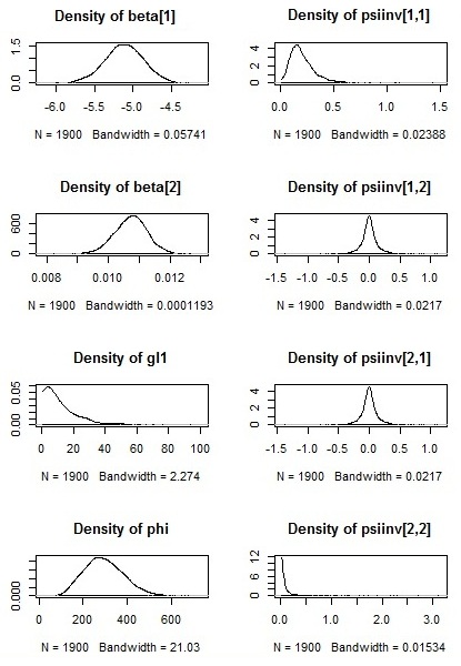
Figure 1: Density; Prater’s data; constant $\phi$; model 1.4

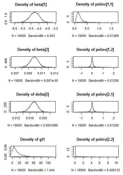
Figure 2: Density; Prater’s data; non constant $\phi$; model 2.5

6 Discussion

Beta regression modeling has gained increasing popularity after the work of Ferrari and Cribari-Neto (2004), who described a beta regression model parameterized in terms of the mean response and a common precision parameter, and developed frequentist inference and basic diagnostic tools for the proposed model. A complementary approach proposed by Smithson and Verkuilen (2006) considers that the precision parameter is not fixed but, instead, is modeled in a regression manner. A Bayesian beta regression model was studied by Branscum et al. (2007). In this paper, we extended these ideas for a mixed beta regression model under a Bayesian perspective.

The present paper considered Bayesian inference for mixed beta regression based on two different approaches. First, the precision parameter was assumed to be fixed, i.e., the same for all observations. A linear regression structure was proposed for the mean parameter through a logit link function. Our results are readily extended to other link choices. Specification of different priors for the common precision parameter was studied. We considered a prior distribution for $\phi$ of the type $\phi=\texttt{U}^{2}$, with $\texttt{U}\sim U(0,a)$, where it is common to consider as initial value $a=50$ (Gelman, 2006). We also proposed alternative priors, namely, prior distributions of the type $\phi=(aB)^{2}$, with $B\sim{\rm beta}(1+\epsilon,1+\epsilon)$ and $\epsilon=0.001,0.01,0.1,0.5,\ldots$, which delivered good results in terms of model fit and performance of diagnostics tests. Second, the precision parameter was modeled through its own linear regression structure using a log link. Again, other choices of the precision link function can be accommodated. For both the mean and the precision submodels, a mixed-effects model with a multivariate $t$ distribution for the fixed and the random effects was considered. Our empirical applications yielded good results in terms of model fit and diagnostic tests. It is worth mentioning that in this context, it is necessary to perform a careful model selection for the precision modeling including more or fewer fixed and random effects since it is not clear in advance which model is more plausible.

A classic version of this problem was raised by Zimprich (2010), where mixed beta regression models were estimated using the SAS procedure NLMIXED (SAS (2008)), employing adaptive Gaussian quadrature. This approach achieves good results, but the implementation of the mixed beta regression model for random effects that are non-normally distributed is very challenging. In this sense, our approach is more flexible because one can easily implement it when the distribution of the random effects follow a normal, Student-$t$, skew normal or another distribution, by using simple and accessible software such as WinBUGS. Another advantage of this approach is the easy implementation for the imputation of missing data (Carrigan et al., 2007), a common situation in practice and for which a classic approach is much more complicated.

Appendix: BUGS codes for the mixed beta regression

This appendix presents the various pieces of BUGS code used for fitting the mixed beta regression in the simulated data example.

Inverse gamma prior for $\phi$

  model
    {
        for( i in 1 : m ) {
        for( j in 1 : n ) {
        Y[i , j] ~ dbeta(a1[i,j] ,a2[i,j])
        a1[i,j] <-  mu[i , j]*phi
        a2[i,j] <- (1-mu[i , j])*phi
        logit(mu[i , j]) <- inprod(x[i, j, ], beta[ ])+inprod(z[i, j, ], b[i,1,])
            }
        b[i,1,1:q ]  ~ dmt(cerovec [ ] ,psi[ , ],gl1)
                }
            gl1~dexp(a0)
        beta[1:p] ~ dmt(alpha[  ] , V1[ , ],gl2)
        V1[1:p ,1:p] <- inverse(V[ , ])
        psi[1:q,1:q] ~ dwish(R0[ , ], c0)
        psiinv[1:q,1:q]<-inverse(psi[1:q,1:q])
        phiinv ~ dgamma(a00,a00)
        phi<-1/phiinv
            }

Uniform prior for $\phi$

  model
    {
        for( i in 1 : m ) {
        for( j in 1 : n ) {
        Y[i , j] ~ dbeta(a1[i,j] ,a2[i,j])
        a1[i,j] <-  mu[i , j]*phi
        a2[i,j] <- (1-mu[i , j])*phi
        logit(mu[i , j]) <- inprod(x[i, j, ], beta[ ])+inprod(z[i, j, ], b[i,1,])
            }
        b[i,1,1:q ]  ~ dmt(cerovec [ ] ,psi[ , ],gl1)
                }
        gl1~dexp(a0)
        beta[1:p] ~ dmt(alpha[  ] , V1[ , ],gl2)
        V1[1:p ,1:p] <- inverse(V[ , ])
        psi[1:q,1:q] ~ dwish(R0[ , ], c0)
        psiinv[1:q,1:q]<-inverse(psi[1:q,1:q])

        phir ~ dunif(a00,b01)
        phi<- phir*phir
            }

Beta prior for $\phi$

  model
    {
        for( i in 1 : m ) {
        for( j in 1 : n ) {
        Y[i , j] ~ dbeta(a1[i,j] ,a2[i,j])
        a1[i,j] <-  mu[i , j]*phi
        a2[i,j] <- (1-mu[i , j])*phi
        logit(mu[i , j]) <- inprod(x[i, j, ], beta[ ])+inprod(z[i, j, ], b[i,1,])
            }
        b[i,1,1:q ]  ~ dmt(cerovec [ ] ,psi[ , ],gl1)
                }
        gl1~dexp(a0)
        beta[1:p] ~ dmt(alpha[  ] , V1[ , ],gl2)
        V1[1:p ,1:p] <- inverse(V[ , ])
        psi[1:q,1:q] ~ dwish(R0[ , ], c0)
        psiinv[1:q,1:q]<-inverse(psi[1:q,1:q])
        phiinicial ~ dbeta(a00,b0)
        phi<-(phiinicial*b11)*(phiinicial*b11)
            }

Submodel for $\phi$

  model
    {
        for( i in 1 : m ) {
        for( j in 1 : n ) {
        Y[i , j] ~ dbeta(a1[i,j] ,a2[i,j])
        a1[i,j] <-  mu[i , j]*phi[i,j]
        a2[i,j] <- (1-mu[i , j])*phi[i,j]
        log(phi[i,j])<-inprod(x[i, j, ], delta[ ])+inprod(z[i, j, ], gama[i,1,])
        logit(mu[i , j]) <- inprod(x[i, j, ], beta[ ])+inprod(z[i, j, ], b[i,1,])
            }
        b[i,1,1:q ]  ~ dmt(cerovec [ ] ,psi[ , ],gl1)
        gama[i,1,1:q ]  ~ dmt(cerovec [ ] ,psi[ , ],gl1)
                }
        gl1~dexp(a0)
        beta[1:p] ~ dmt(alpha[  ] , V1[ , ],gl2)
        delta[1:p] ~ dmt(alpha[  ] , V1[ , ],gl2)
        V1[1:p ,1:p] <- inverse(V[ , ])
        psi[1:q,1:q] ~ dwish(R0[ , ], c0)
        psiinv[1:q,1:q]<-inverse(psi[1:q,1:q])
        meanphi<-mean(phi[,])
            }

References

References

- Albert and Chib (1993) Albert, J. H., Chib, S., 1993. Bayesian analysis of binary and polychotomous response data. Journal of the American Statistical Association 88, 669–679.
- Besag et al. (1995) Besag, J., Green, P., Higdon, D., Mengersen, K., 1995. Bayesian computation and stochastic systems. Statistical Science 10, 3–66.
- Branscum et al. (2007) Branscum, A. J., Johnson, O. J., C.Thurmond, M., 2007. Bayesian beta regression: applications to household expenditure data and genetic distance between foot-and-mouth disease viruses. Australian and New Zealand Journal of Statistics 49, 287–301.
- Brooks (2002) Brooks, S. P., 2002. Discussion on the paper by spiegelhalter, best, carlin, and van der linde (2002). Journal of the Royal Statistical Society B 64, 616 618.
- Brooks and Gelman (1998) Brooks, S. P., Gelman, A., 1998. General methods for monitoring convergence of iterative simulations. Journal of Computational and Graphical Statistics 7, 434–455.
- Carlin and Louis (2001) Carlin, B. P., Louis, T. A., 2001. Bayes and Empirical Bayes Methods for Data Analysis. Chapman and Hall, Boca Raton.
- Carrigan et al. (2007) Carrigan, G., Barnett, A., Dobson, A. J., Mishra, G., 2007. Compensating for missing data from longitudinal studies using winbugs. Journal of Statistical Software 19, issue 7.
- Dey et al. (2000) Dey, D. K., Ghosh, S. K., Mallick, B. K., 2000. Generalized Linear Models: A Bayesian Perspective, 1st Edition. Marcel Dekker, New York.
- Everson and Morris (2000) Everson, P. J., Morris, C. N., 2000. Inference for multivariate normal hierarchical models. Journal of the Royal Statistical Society B 62 (Part 2), 399–412.
- Ferrari and Cribari-Neto (2004) Ferrari, S. L. P., Cribari-Neto, F., 2004. Beta regression for modelling rates and proportions. Journal of Applied Statistics 31, 799–815.
- Fong et al. (2010) Fong, Y., Rue, H., Wakefield, J., 2010. Bayesian inference for generalized linear mixed models. Biostatistics 11, 397–412.
- Gelman (2006) Gelman, A., 2006. Prior distributions for variance parameters in hierarchical models. Bayesian Analysis 1, 515–533.
- Gelman and Rubin (1992) Gelman, A., Rubin, D. B., 1992. Inference from iterative simulation using multiple sequences. Statistical Science 7, 457–511.
- Geweke (1992) Geweke, J., 1992. Evaluating the accuracy of sampling-based approaches to calculating posterior moments. In Bayesian Statistics 4 (ed JM Bernado, JO Berger, AP Dawid and AFM Smith), 169–193.
- Geweke (1993) Geweke, J., 1993. Bayesian treatment of the independent Student-t linear model. Journal of Applied Econometrics S8, 19–40.
- Heidelberger and Welch (1981) Heidelberger, P., Welch, P. D., 1981. A spectral method for confidence interval generation and run length control in simulations. Communications of the ACM 24, 233–245.
- Heidelberger and Welch (1983) Heidelberger, P., Welch, P. D., 1983. Simulation run length control in the presence of an initial transient. Operations Research 31 - 6, 1109–1144.
- Plummer et al. (2006) Plummer, M., Best, N., Cowles, K., Vines, K., 2006. The coda package. R Project. http://cran.r-project.org/doc/packages/coda.pdf.
- Prater (1956) Prater, N. H., 1956. Estimate gasoline yields from crudes. Petroleum Refiner 35, 236–238.
- SAS (2008) SAS, 2008. SAS/STAT 9.2 User s Guide. Cary, NC.
- Smithson and Verkuilen (2006) Smithson, M., Verkuilen, J., 2006. A better lemon squeezer? Maximum-likelihood regression with beta-distributed dependent variables. Psychological Methods 11, 54–71.
- Spiegelhalter et al. (2002) Spiegelhalter, D., Best, N., Carlin, B., Linde, A., 2002. Bayesian measures of model complexity and fit. Journal of the Royal Statistical Society B 64, 583–639.
-
Venables (2000)
Venables, W. N., 2000. Exegeses on linear models. Paper available at
http://www.stats.ox.ac.uk/pub/MASS3/Exegeses.pdf. - Zimprich (2010) Zimprich, D., 2010. Modeling change in skewed variables using mixed beta regression models. Research in Human Development 7, 9–26.