The ATCA H i Survey of the Galactic Center

Abstract

We present a survey of atomic hydrogen (H i) emission in the direction of the Galactic Center conducted with the CSIRO Australia Telescope Compact Array (ATCA). The survey covers the area $-5\arcdeg\leq l\leq+5\arcdeg$, $-5\arcdeg\leq b\leq+5\arcdeg$ over the velocity range $-309\leq v_{LSR}\leq 349$ ${\rm km~{}s^{-1}}$ with a velocity resolution of 1 ${\rm km~{}s^{-1}}$. The ATCA data are supplemented with data from the Parkes Radio Telescope for sensitivity to all angular scales larger than the $145\arcsec$ angular resolution of the survey. The mean rms brightness temperature across the field is $0.7$ K, except near $(l,b)=0\arcdeg,0\arcdeg$ where it increases to $\sim 2$ K. This survey complements the Southern Galactic Plane Survey to complete the continuous coverage of the inner Galactic plane in H i at $\sim 2\arcmin$ resolution. Here we describe the observations and analysis of this Galactic Center survey and present the final data product. Features such as Bania’s Clump 2, the far 3 kiloparsec arm and small high velocity clumps are briefly described.

1 Introduction

The central 3 kiloparsecs of the Milky Way contain information on a wealth of astrophysical processes from Galactic dynamics to Galactic outflows. The extended environment of the Galactic Center (GC) provides an outstanding opportunity to study the dynamics of gas flow in a barred Galaxy and the relationship of molecular and atomic gas in the unique GC environment. Atomic hydrogen (H i) observations of this region offer a clear view of the gas dynamics at the center of our Galaxy, probing the transition between orbits associated with the bar, circular orbits, and the beginnings of the spiral arms.

The spatial distribution of interstellar matter in the innermost 3 kpc has recently been reviewed by Morris & Serabyn (1996) and Ferrière et al. (2007). The main structural features that make up the GC region have been discussed extensively in the literature, including reviews by Blitz et al. (1993) and Genzel et al. (1994). Amongst the main structural features inside the GC are: both a long, thin bar (Hammersley et al., 2000; Benjamin et al., 2005; Cabrera-Lavers et al., 2008) and a short, boxy-bulge bar (e.g. Blitz & Spergel, 1991; Dwek et al., 1995; Babusiaux & Gilmore, 2005); the near 3 kpc arm (van Woerden et al., 1957; Oort et al., 1958); and the Central Molecular Zone (CMZ) covering the inner 150 - 250 pc (Morris & Serabyn, 1996).  More recently discovered features include the far-side 3 kpc arm (Dame & Thaddeus, 2008), and a thin twisted 100 pc ring (Sawada et al., 2004; Martin et al., 2004; Liszt, 2008; Molinari et al., 2011).

Studies of the dynamics of gas, including high resolution CO observations (e.g Liszt & Burton, 1978; Burton & Liszt, 1992; Oka et al., 1998) and high sensitivity, low resolution H i (Liszt & Burton, 1980), detail the distribution and kinematics of molecular gas in the CMZ. These data have constrained extensive models of the dynamics of the GC, including those incorporating the effects of the bar(s) (e.g. Peters, 1975; Binney et al., 1991; Fux, 1999; Rodriguez-Fernandez et al., 2006; Romero-Gómez et al., 2011).

In addition to Galactic dynamics, H i observations of the GC region may reveal any putative gas outflows from the GC. Much of the early analysis of the GC H i invoked large-scale gas expulsive events (van der Kruit, 1970, 1971; Sanders & Wrixon, 1972) to explain the highly non-circular motions observed in the H i emission envelope. Since Liszt & Burton (1980) showed that the forbidden velocity gas and its prevalence off the Galactic mid-plane could be explained by a tilted-bar inducing elliptical gas streamlines the idea of large-scale neutral gas outflows has largely disappeared. However, due to lack of high-resolution data probing small physical scales there is very little information about any small-scale outflows associated with star formation at the GC. For example, we know nothing about whether there is H i associated with the Galactic wind suggested by Bland-Hawthorn & Cohen (2003), despite evidence for cool and warm gas in the wind.

Large-scale surveys of the distribution of atomic hydrogen around the GC have a long history and include observations with the Dwingeloo 26m (van Woerden et al., 1957; van der Kruit, 1970), the Parkes 18m (Kerr, 1967), an extensive Jodrell Bank survey of $355\arcdeg\leq l\leq 10\arcdeg$, $|b|\leq 5\arcdeg$, $|v|\leq 530$ ${\rm km~{}s^{-1}}$ (Cohen, 1975), the NRAO 140-ft survey of $349\arcdeg\leq l\leq 13\arcdeg$, $|b|\leq 10\arcdeg$, $|v|\leq 350$ ${\rm km~{}s^{-1}}$ (Burton & Liszt, 1978; Liszt & Burton, 1980; Burton & Liszt, 1983) and the recent all-sky H i surveys: the Leiden-Argentine-Bonn survey (Kalberla et al., 2005) and the Galactic All-Sky Survey (McClure-Griffiths et al., 2009; Kalberla et al., 2010). Although the H i in the GC has been well-studied at low resolution, the large-scale environment is relatively untapped at angular resolutions better than $>0.25\arcdeg$. Braunfurth & Rohlfs (1981) conducted a slightly higher resolution, limited area, survey of $|l|\leq 1.5\arcdeg$, $|b|\leq 1.5\arcdeg$ with the Effelsberg 100m telescope, with a sampling grid and beamsize of $0.15\arcdeg$. More recently Lang et al. (2010) produced a high angular resolution survey of H i absorption, but only in the central $100\arcmin\times 50\arcmin$. Hence, there are currently no high-resolution H i datasets covering the entire GC region to compare with detailed dynamical models and theories of molecular transition (about 180–250 pc from the GC, outside the CMZ, the nuclear disk has been thought to transition from molecular hydrogen to H i (Liszt & Burton 1978; Bitran et al. 1997; Morris & Serabyn 1996)). Furthermore, the angular resolution of new infrared data on the GC from Spitzer (Arendt et al., 2008) and Herschel (Molinari et al., 2010, 2011) exceeds the resolution of existing H i data of the inner 3 kpc by more than an order of magnitude.

In this paper we describe the atomic hydrogen (H i) component of a survey of the Galactic Center conducted with the Australia Telescope Compact Array and incorporating single dish data from Parkes. Here we take an intermediate approach, covering an area of $10^{\circ}\times 10^{\circ}$ around the Galactic Center with an angular resolution of $145$ arcseconds in atomic hydrogen (H i) and in 20 cm continuum. At a distance of 8.4 kpc (Ghez et al., 2008; Reid et al., 2009) the survey covers about 1500 pc on all sides of the Galactic Center with a spatial resolution of about 6 pc. This survey builds on the Southern Galactic Plane Survey (SGPS; McClure-Griffiths et al., 2005), VLA Galactic Plane Survey (VGPS; Stil et al., 2006) and Canadian Galactic Plane Survey (CGPS; Taylor et al., 2003) to complete the International Galactic Plane Survey of the first, second and fourth Galactic quadrants. We discuss the observations and data reduction of our Galactic Center H i survey (§2 & §3), present the data cubes (§4) and discuss noteworthy features (§5). The data have been made publicly available at: http://www.atnf.csiro.au/research/HI/sgps/GalacticCenter.

2 ATCA Observations

The Galactic Center survey data were obtained with the Australia Telescope Compact Array (ATCA) and the Parkes Radio Telescope. The Parkes data are from the Galactic All-Sky Survey (McClure-Griffiths et al., 2009; Kalberla et al., 2010) and are described therein. The ATCA observations were conducted between December 2002 and March 2004. The ATCA consists of five moveable 22-m antennas on a 3-km east-west track and an additional 22-m antenna at a fixed position 3-km west of the end of the track. Observations were conducted in six different array configurations: EW352, EW367, 750A, 750B, 750C, and 750D. The array configurations were chosen to give optimum coverage of the inner u-v plane out to a baseline of 750 m. Data were recorded from the sixth antenna, with a maximum baseline of 6 km, but these are not used in the image cubes presented here. The shortest baseline is 31 m and every baseline, in intervals of 15.5m, to 245 m is sampled

To image the full $10^{\circ}\times 10^{\circ}$ area the survey was conducted as a mosaic of many pointings. The primary beam of the ATCA antennas, $\lambda/D=33^{\prime}$, determines the optimum spacing between pointings, where $\lambda=21$ cm is the observing wavelength and $D=22~{}{\rm m}$ is the ATCA antenna diameter. The mosaic pointings were arranged on a hexagonal grid with a separation of 20^′. Although this is slightly wider than the optimum hexagonal spacing of $(2/\sqrt{3})(\lambda/2D)\sim 19\arcmin$, the theoretical sensitivity varies by less than 2% across the field. A total of 1031 pointings were required to cover the full area; 64 of these were previously observed as part of the Southern Galactic Plane Survey (McClure-Griffiths et al., 2005). The 64 SGPS pointings were re-observed several times with the 750A and 750D arrays as part of the Galactic Center project to help improve the u-v sampling of the longer baselines. The overall observing strategy was similar to that used for the SGPS and described by McClure-Griffiths et al. (2005). The 967 new pointings were observed in 60s integrations approximately 25 times at widely spread hour angles. We chose 60s integrations to mitigate against the effects of fluctuating sampler statistics caused by mosaicing very strong continuum sources. In practice we found the first 10s sample was occasionally flagged as bad because of sample statistics when the mosaic centre was moved to some of the pointings closest to $(l,b)\approx(0\arcdeg,0\arcdeg)$; samplers did not cause problems for the majority of the pointings. The 967 pointings were divided into subfields of 42 or 36 pointings that were observed as continuous blocks. Within each of these blocks the u-v coverage and integration time was essentially the same for all pointings. Multiple blocks were observed during the course of each observing day and care was taken to ensure that the hour angle coverage for each block was as uniform as possible. An example of the u-v coverage for a pointing in the north-western corner of the field is shown in Figure 1.

The ATCA has linear feeds, recording two orthogonal linear polarizations, $X$ and $Y$. These data were obtained prior to the Compact Array Broadband Backend upgrade (Wilson et al., 2011), and therefore were recorded simultaneously in a narrowband spectral line mode with 1024 channels across a 4 MHz bandwidth centered on 1420 MHz and a broadband mode recording 32 channels across a 128 MHz bandwidth centered on 1384 MHz. For the narrowband mode that is the focus of this paper, only auto correlations, $XX$ and $YY$ were recorded. All four polarization products, $XX$, $YY$, $XY$, and $YX$ were recorded in the broadband mode. The broadband data will be the subject of a future paper.

3 Calibration and Imaging

Data editing, calibration and imaging were performed in the Miriad package using standard techniques (Sault et al., 1995). The ATCA’s primary flux calibrator, PKS B1934-638, was observed at least once per day. PKS B1934-638 was used for bandpass calibration and primary flux calibration assuming a flux of 14.86 Jy at 1420 MHz (Reynolds, 1994). In addition, a secondary calibrator, PKS B1827-360, was observed for 2 minutes every $\sim 1$ hr to solve for time varying complex gains. Gain solutions determined on PKS 1827-360 were copied across to the Galactic Center pointings.

Data-editing, or flagging, was carried out by hand within Miriad. Although the 4 MHz band around the H i line is generally free from significant radio-frequency interference (RFI) there was some intermittent locally generated RFI at 1420.0 MHz, apparent on the shortest baselines. This was flagged by hand and after Doppler correction the flagged frequency channels were spread around many velocity channels. However, in some cases the 1420.0 MHz RFI constituted a significant amount of the short baseline data for channels in the velocity range $95~{}{\rm km~{}s^{-1}}\lesssim v\lesssim 105~{}{\rm km~{}s^{-1}}$. For these channels the noise in the final images is slightly higher and the image fidelity is generally worse than in other parts of the dataset due to poor u-v sampling.

Continuum emission was subtracted from the data in the u-v plane using a linear fit to ranges of channels on either side of the main H i line (Sault, 1994). The ATCA does not Doppler track so Doppler corrections were applied to the data after calibration and continuum subtraction and before imaging. The data were shifted to the IAU defined Local Standard of Rest (LSR) assuming a solar velocity $V_{sun}=20.0$ ${\rm km~{}s^{-1}}$ in the direction of $RA=18^{h}07^{m}50.3^{s}$, $\delta=+30^{\circ}00^{\prime}52^{\prime\prime}$, J2000.0. The continuum subtracted data of the individual 1031 pointings were linearly combined to form a dirty image of the entire field. This approach to mosaicing, rather than the approach of combining the pointings after deconvolution, is most effective at recovering information on the largest angular scales. Robust weighting, with a robust factor of +0.7, was used in the imaging. This robustness was found to optimize the sidelobe levels, synthesized beam size and overall noise for these images.

The Galactic Center region contains several very strong continuum sources which, when seen in absorption, appear as negative sources in the continuum subtracted H i line cubes. For the sources near $(l,b)=(0.0^{\circ},0.0^{\circ})$ (Sgr A), $(l,b)=(0.86^{\circ},0.07^{\circ})$ (Sgr B2) and $(l,b)=(0.6^{\circ},-0.05^{\circ})$ (Sgr B) the continuum flux is sufficient that absorption is observed in almost every channel where there is H i emission. The maximum entropy deconvolution techniques traditionally used for large Galactic H i mosaics are not sufficient to deconvolve diffuse emission in the presence of strong negative sources. The standard maximum entropy technique has a positivity constraint, which means that rather than deconvolving the strongly negative sources, the sidelobes for these would be treated as structure in the H i emission and the algorithm would attempt to deconvolve these structures.

In order to deconvolve the H i cube we used a combined approach of maximum entropy and traditional CLEAN (Högbom, 1974). Before deconvolution of the diffuse H i emission we deconvolved the strongest negative sources using the clean algorithm in Miriad’s MOSSDI. Differing from the technique employed by Stil et al. (2006), we did not filter out small u-v distances because the continuum structure near ($l,b$) = ($0.0\arcdeg,0.0\arcdeg$) is extended and the absorbed flux exceeds that of the diffuse emission by a factor of $\sim 20$. After deconvolving the absorbed emission, and taking care to not iterate so far as to start cleaning the diffuse emission, the clean-component model was subtracted from the u-v data. The resulting data were then re-imaged and the H i emission deconvolved using Miriad’s maximum entropy algorithm, MOSMEM. To construct the final image cube we first created a ’residual’ cube. The residual is the difference of the clean-component model of the u-v subtracted dirty cube and the maximum entropy model convolved with the dirty beam. This residual image cube was then combined with the clean and maximum entropy models convolved with a circular Gaussian of 145^′′. This combined maximum entropy and traditional clean technique proved quite effective, removing most of the sidelobe structure around the strongest continuum sources near $-0.2^{\circ}\leq l\leq 0.2^{\circ}$, $-0.2^{\circ}\leq b\leq 0.2^{\circ}$, plus toward $(l,b)=(0.86^{\circ},0.07^{\circ})$ and $(l,b)=(0.6^{\circ},-0.05^{\circ})$.

3.1 Single-dish and Interferometer Combination

Although mosaicing recovers information on angular scales up to $\lambda/(d_{min}-D/2)\sim 36^{\prime}$, where $d_{min}=31~{}{\rm m}$ is the minimum baseline measured and $D=22~{}{\rm m}$ for the ATCA, information on larger angular scales is lost to the interferometer. To recover information on larger angular scales it has become common practice to combine the interferometric data with images from a single-dish telescope. For this survey we use H i data cubes from the Parkes Galactic All-Sky Survey (GASS; McClure-Griffiths et al., 2009; Kalberla et al., 2010), which have an angular resolution of 16′ and the same velocity resolution as the ATCA data (1 ${\rm km~{}s^{-1}}$). The GASS data are significantly more sensitive than the ATCA data, with an rms brightness temperature of $\sim 55$ mK, and therefore do not contribute significantly to the final noise of the survey presented here.

There are a number of techniques for combining single dish and interferometric data, including combination prior to deconvolution, during deconvolution and after deconvolution. The techniques and the merits of each are described in detail by Stanimirović (2002). For ATCA data with moderate u-v sampling, experience has shown that the most robust technique is to combine the images in the Fourier domain after deconvolution. As implemented in Miriad’s IMMERGE, the single dish and interferometric data are deconvolved separately, then Fourier transformed, reweighted, linearly combined and then inverse Fourier transformed. Mathematically, the Fourier transform of the combined image, $V_{comb}$ can be expressed as:

$$V_{comb}(k)=\omega^{\prime}(k)V_{int}(k)+f_{cal}\omega^{\prime\prime}(k)V_{sd}(k),$$ (1)

where $V_{int}(k)$ is the Fourier transform of the deconvolved ATCA mosaic and $V_{sd}(k)$ is the Fourier transform of the deconvolved Parkes image. The weighting functions, $\omega^{\prime}(k)$ and $\omega^{\prime\prime}(k)$, are defined such that $\omega^{\prime}(k)+\omega^{\prime\prime}(k)$ is a Gaussian whose full width at half-maximum is the same as the synthesized ATCA beam. In this way the ATCA data are down-weighted at the large angular scales and the Parkes data are down-weighted at the small angular scales. The calibration factor, $f_{cal}$, scales the Parkes data to match the flux scale of the ATCA data. This factor is determined by comparing the ATCA and Parkes images at every pixel and frequency in the range of overlapping spatial frequencies, which for an ATCA mosaic and a Parkes image is $120\lambda$ to $190\lambda$, for $\lambda=21$ cm. For GASS data and our ATCA image we found a calibration factor $f_{cal}=1.2$.

4 Data product

The final combined H i cube was regridded to Galactic coordinates and converted to Kelvins of brightness temperature, assuming filled emission on the scale of the ATCA synthesized beam. The cube covers the area $-5.1^{\circ}\leq l\leq+5.1^{\circ}$, $-5.1^{\circ}\leq b\leq 5.1^{\circ}$ with a pixel size of 35″ and a beam size of 145″. The velocity coverage is $-309~{}{\rm km~{}s^{-1}}\leq v\leq 349~{}{\rm km~{}s^{-1}}$ with a channel spacing of $0.82$ ${\rm km~{}s^{-1}}$ and an effective velocity resolution of 1 ${\rm km~{}s^{-1}}$.

4.1 Data Quality and Artifacts

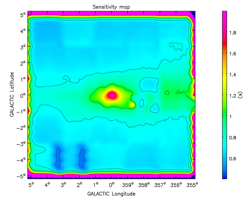
Figure 2: Sensitivity map of the survey region. The color scale is shown in the wedge at the right and varies linearly from 0.6 - 2.5 K. The contours are at 0.5 - 2.0 K in increments of 0.25 K. The sensitivity is not completely uniform due to: (1) slightly uneven u-v coverage of the individual fields that make up the mosaic and (2) bright continuum sources, which increase the system temperature and (3) broad H i linewidths toward $b=0\arcdeg$, which occupy a large fraction of the observing bandwidth and increase the system temperature.

The sensitivity in the data cube varies slightly across the field because of observing strategy used to cover the subregions. Figure 2 is an image of the rms brightness temperature sensitivity per channel created from the expected sensitivity based on the per pointing integration time, scaled to the actual sensitivity as measured from the rms in off-line regions of the cube. Variations in rectangular patches are due to differences in the total number of snapshots on each sub-field. The remaining variations, in particular the increased rms towards the Galactic Center and around the Galactic plane, in general are due to true increases in system temperature from the contributions of the strong continuum emission and bright H i, which fills most of the velocity band. The mean rms, $\sigma_{tb}$, per channel away from the Galactic plane is $\sim 0.7$ K, increasing to $\sim 1.0$ K at $b\sim 0\arcdeg$ and $\sim 2.0$ K towards $(l,b)=(0.0\arcdeg,0.0\arcdeg)$.

In general the mean rms measured in individual off-line channels is comparable to the channel-to-channel rms measured in individual spectra. However, the spatial distribution of the noise is not entirely constant with velocity. The velocity coverage differs slightly from field to field and particularly for the data incorporated from the SGPS, which covered a slightly smaller range. As a result the noise increases for $v<-225$ ${\rm km~{}s^{-1}}$ and $v>267$ ${\rm km~{}s^{-1}}$ in the region that was originally covered by the SGPS, namely $l<-3\arcdeg$, $|b|<1.2\arcdeg$.

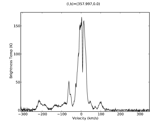
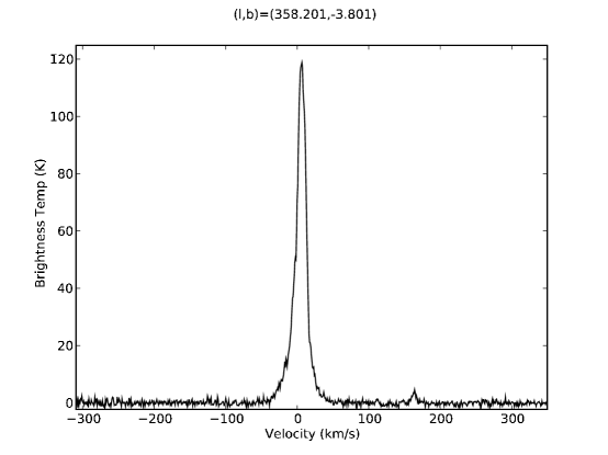
Figure 3: Example spectra towards two positions, near ($l,b=-2.0\arcdeg,0.0\arcdeg$) and far ($l,b=-1.8\arcdeg,-3.8\arcdeg$) from the Galactic plane. These spectra give an indication of the noise in the spectral domain and the spectral baselines.

Figure 3 shows two example spectra at $(l,b)=(358.0\arcdeg,0\arcdeg)$ and $(l,b)=(358.2\arcdeg,-3.8\arcdeg)$. These demonstrate the spectral baseline quality and spectral noise achieved in this survey. The slight increase in rms at the extreme velocities is apparent in the spectrum obtained at $(l,b)=(358.0\arcdeg,0\arcdeg)$.

The data cube contains some imaging artifacts. These fall into two main categories: those associated with strongly absorbed continuum sources, and low-level artifacts due to limited u-v coverage that lie near the noise level in individual channels. The most obvious imaging artifacts are those due to dynamic range limitations around the strongly absorbed continuum sources near $(l,b)=(0\arcdeg,0\arcdeg$) and $(l,b)=(-2.4\arcdeg,-0.1\arcdeg)$. These regions are limited by incomplete cleaning, a problem that cannot be solved with the deconvolution techniques used here, but may be addressed in the future using Multi-scale clean (Cornwell, 2008). There are a few pixels at $(l,b)\approx(0\arcdeg,0\arcdeg$) in the GASS data that were saturated in the raw data at the time of observation. The limited dynamic range of the area immediately surrounding Sgr A^∗, plus the lack of an accurate single dish image at this position, limits the usefulness of this dataset for studying the H i absorption towards Sgr A^∗. For studies of absorption in the inner degree, users are advised to use the Lang et al. (2010) VLA survey.

The other category of imaging artifacts is apparent in images created by integrating over large velocity ranges such as zeroth moment images, which show residual striping and cross-hatching. These effects are almost certainly due to the limited u-v coverage, although some of the more prominent regions of parallel striping are clearly due to low-level RFI that has not been completely flagged. In individual velocity channels these effects mostly lie below the noise.

Small spurious emission features appear at a velocity of $v=+48$ ${\rm km~{}s^{-1}}$ at $(l,b)=(3.77\arcdeg,-2.24\arcdeg)$, $(l,b)=(4.13\arcdeg,-2.57\arcdeg)$ and $(l,b)=(4.03\arcdeg,-1.73\arcdeg)$. These bright, $T_{b}\sim 25$ K, features are only three velocity channels wide and are artifacts from the GASS data. No counterparts to these features are observed in the ATCA-only data.

5 Images

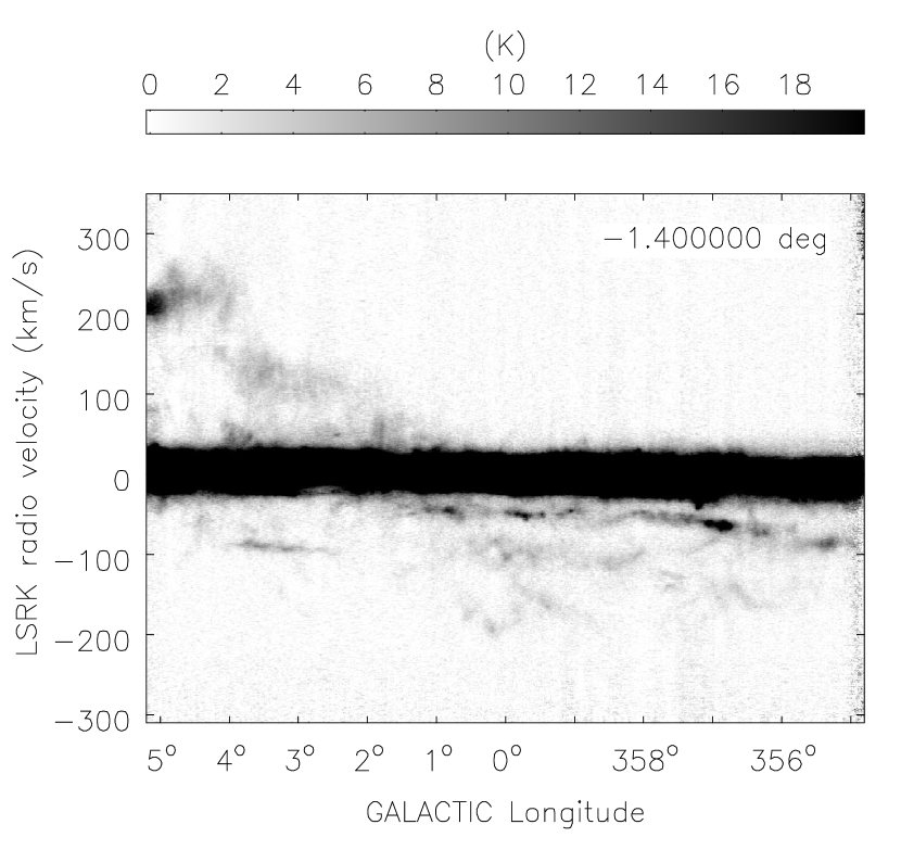
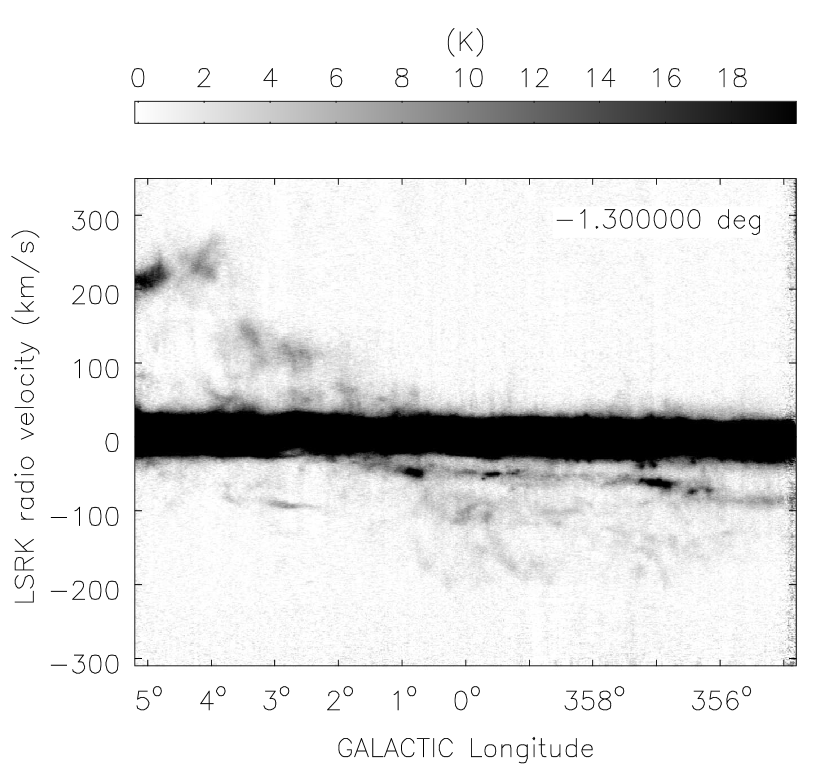
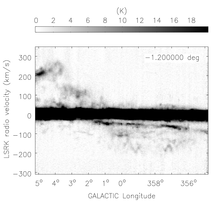
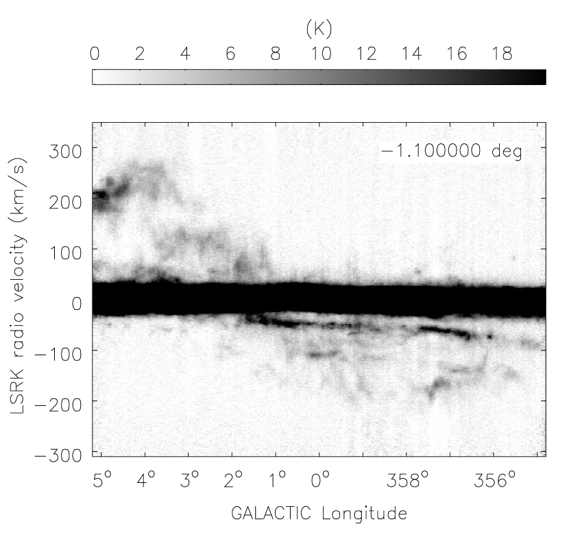
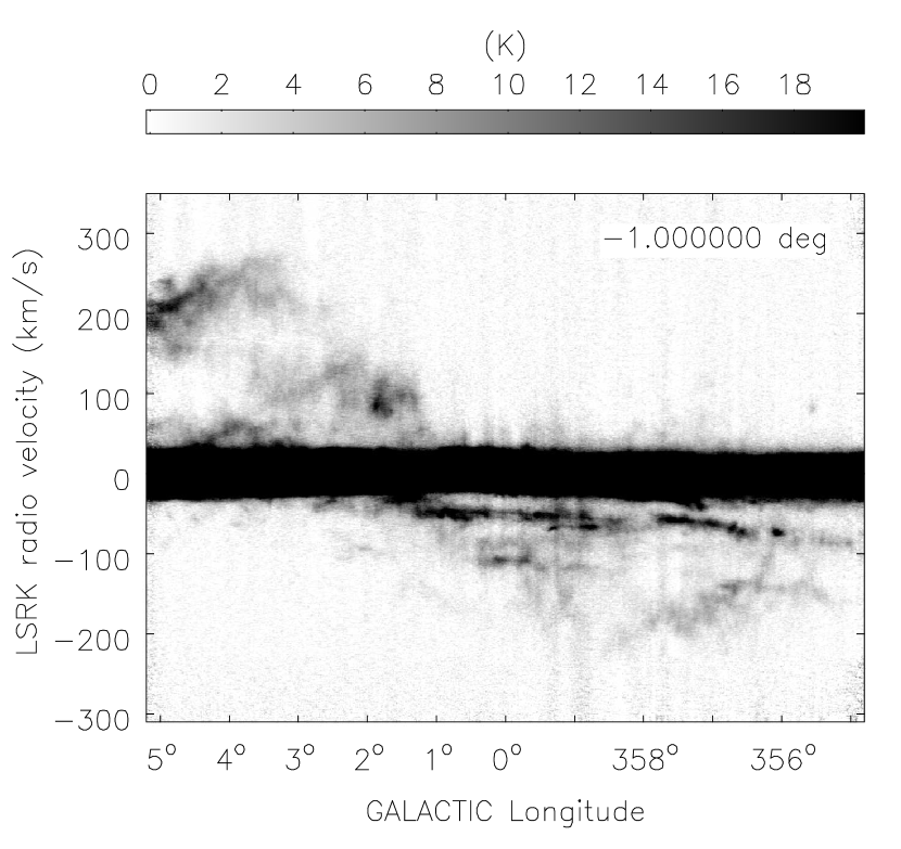
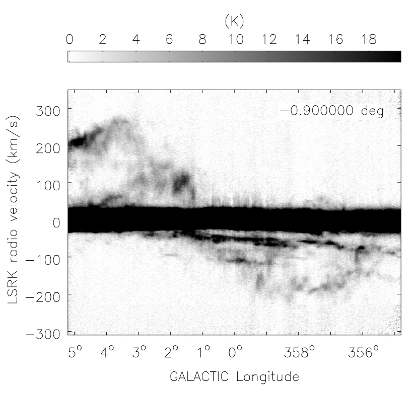
Figure 13: Longitude-velocity images sampled at latitude intervals of $0.1^{\circ}$. The greyscale for each panel is shown in the color wedges, each panel uses a different scaling.

Images of every tenth velocity channel are shown in Figure 4. The greyscale is different for each panel as shown in the associated color wedges. The images highlight the wealth of small-scale features visible in these data. In Figure 13 we show longitude-velocity (l-v) images at latitude intervals of $0.1\arcdeg$ over the latitude range $-1.4\arcdeg\leq b\leq+1.5\arcdeg$. These are especially useful for studying the large-scale structure of the region and can be compared usefully with existing CO data (e.g. Bally et al., 1987; Oka et al., 1998).

5.1 Noteworthy features

Full analysis of these data will focus on the H i structure and dynamics of the Galactic Center and an analysis of individual high-velocity features. These will be the topics of forthcoming papers. Here we restrict ourselves to a brief discussion of some of the most noteworthy features.

5.1.1 Large-scale H i Distribution

Figure 4 shows the H i sky distribution sampled every 8 ${\rm km~{}s^{-1}}$. The high velocities ($|v|>100$ ${\rm km~{}s^{-1}}$) show the well known (e.g. Kerr, 1967; van der Kruit, 1970; Burton & Liszt, 1978) H i emission structure of positive velocity gas at $b<0\arcdeg$ and $l>0\arcdeg$ and similarly, negative velocity gas at $b>0\arcdeg$ and $l<0\arcdeg$. Burton & Liszt (1978) and Liszt & Burton (1980) have attributed this to a tilted H i inner disk which is oriented at 24° with respect to the Galactic plane.

Other well-known features are seen in the longitude-velocity (l-v) images shown in Figure 13, which are sampled at intervals of $0.1^{\circ}$ in latitude. In these we can see the prominent “connecting arm” at extreme positive longitudes and positive velocities ($l>3\arcdeg$, $200~{}{\rm km~{}s^{-1}}\leq v\leq 300~{}{\rm km~{}s^{-1}}$) and the nearly symmetric “looping” ridge at the extreme negative longitudes and velocities ($l<-1\arcdeg$, $v\sim-210~{}{\rm km~{}s^{-1}}$) . Fux (1999) modeled these features as dust lanes on the near and far side of the bar, respectively. The near-side dust lane is particularly prominent at negative longitudes, whereas the far-side lane becomes quite clear at $b\approx 0^{\circ}$.

5.1.2 The 3-kpc arms

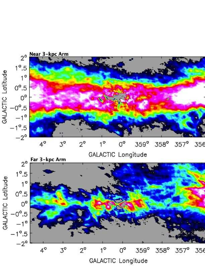
Figure 18: Velocity integrated H i intensity maps of the near (top) and far (bottom) 3-kpc arms following the definitions of Dame & Thaddeus (2008). Emission was integrated over 26 km/s bins, centered at each longitude on the arm at a velocity as defined by the linear fits of Dame & Thaddeus (2008): $v_{lsr}=-53.1+4.16l$ ${\rm km~{}s^{-1}}$ for the near arm and $v_{lsr}=+56.0+4.08l$ ${\rm km~{}s^{-1}}$ for the far arm.

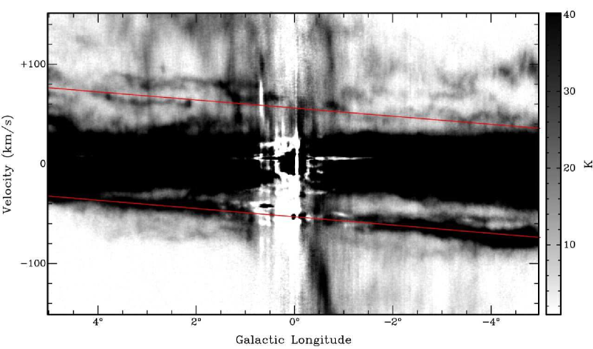
Figure 19: Longitude-velocity at $b=0^{\circ}$ with red lines showing the linear fits of the 3-kpc arms from Dame & Thaddeus (2008).

While the near 3-kpc arm has been well studied in H i at low resolution, both the near 3-kpc arm and the recently discovered far 3-kpc arm are unexplored in H i at this resolution. Following the linear l-v fits of Dame & Thaddeus (2008) we constructed zeroth order moment maps of the H i emission centered on the velocity mid-point of the near and far arms at every longitude within the Galactic centre region, using a width in velocity of 26 ${\rm km~{}s^{-1}}$ as used by Dame & Thaddeus (2008). These are shown in Figure 18. For most of the longitude range covered by our Galactic Center survey the H i emission from the far arm is blended in longitude and latitude with both local gas and gas far outside the solar circle. While the near arm is clearly visible in our data, the far arm is obviously confused by the Galactic centre gas ($l=\pm$1^∘) and also gas near $l\approx 3^{\circ}$, which is associated with Bania’s Clump 2 (see §5.1.3 below). In the intermediate longitudes, particularly near $l=2\arcdeg$ and $l=-2\arcdeg$, there is a narrow strip of emission at $b\approx 0\arcdeg$ which may be attributed to the far 3 kpc arm. We note, however, that the best evidence for the far 3-kpc arm presented by Dame & Thaddeus (2008) lies outside the longitude range of our survey. Figure 19 is a longitude-velocity (l-v) diagram at $b=0^{\circ}$ with the linear fits of Dame & Thaddeus (2008) overlaid. The near 3-kpc arm is clearly visible and hints of the feature identified as the far 3-kpc arm by Dame & Thaddeus (2008) are also visible. The latter shows evidence of a possible split/bifurcation near $l\approx 3\arcdeg$, as was discussed by Dame & Thaddeus (2008).

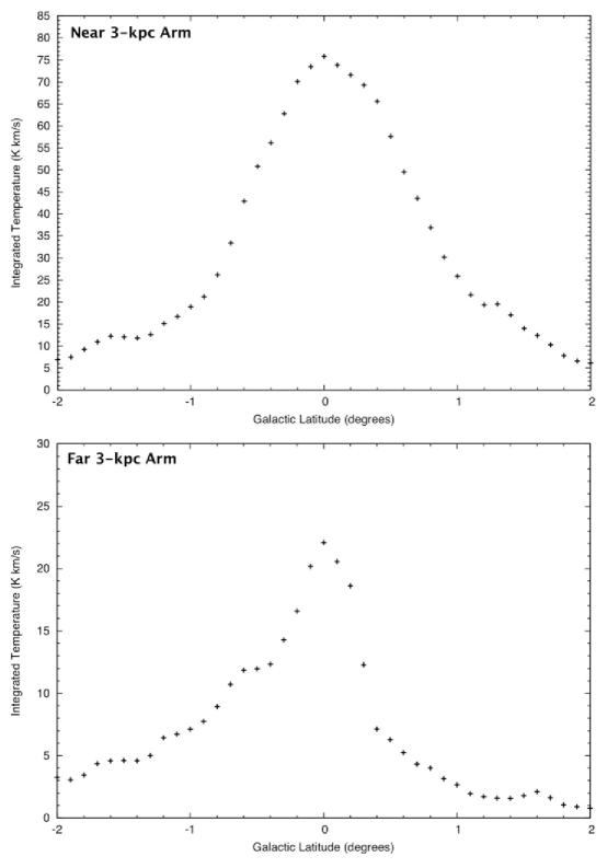
Figure 20: Latitude profiles of the integrated H i emission from the near (top) and far (bottom) 3-kpc arms. The unrelated blended and vertical sections discussed in Dame & Thaddeus (2008) have been excluded.

In Figure 20, we show the integrated latitude profiles of the features shown in Figure 18. These are summed from the non-confused portions of each feature, and as such the far 3-kpc arm latitude profile contains H i emission from only about 2 degrees of longitude. As Dame & Thaddeus (2008) found for the CO emission, the latitude widths of the two arms in differ by a factor of $\sim$2, with full-widths at half-max (FWHMs) in H i of 1.6^∘ and 0.7^∘ for the near and far arms, respectively. Assuming a distance of the 3-kpc arm structure from the Galactic centre of 3.5 to 4 kpc, and a solar distance of 8.4 kpc (Ghez et al., 2008; Reid et al., 2009), these correspond to a FWHM in $z$ of $126-141$ pc and $149-155$ pc for the near and far arms, respectively. Our values differ slightly from the estimates of Dame & Thaddeus (2008), which were calculated over the longitude range $5\arcdeg\leq l\leq 9\arcdeg$ and using slightly different estimates for the solar distance and Galactocentric radius of the 3-kpc arms. If we use the same distance values as Dame & Thaddeus (2008) (5.2 kpc and 11.8 kpc) we find $z$ FWHM values of 149 and 146, respectively. Dame & Thaddeus (2008) used the comparable $z$ heights of the two features as evidence for the far 3kpc arm. They also postulated that the small FWHM is due to a lack of star formation to heat and inflate the gas. However Green et al. (2009) showed high-mass star formation to be present in both arms through the association of 6.7-GHz methanol masers, known tracers of high-mass star formation. This implies that both arms have undergone star formation activity and any effect on $z$ height is the same for both.

5.1.3 Bania’s Clump 2

There are a few positions in the Galactic Center region that are known to have very wide linewidths over an extent $>0.5\arcdeg$ (Bania, 1977). These have been observed extensively in ¹²CO (Bania et al., 1986; Stark & Bania, 1986; Liszt, 2006), OH (Boyce & Cohen, 1994) and other molecular line tracers (Lee, 1996; Huettemeister et al., 1998; Liszt, 2006), as well as in H i (eg. Riffert et al., 1997). The area known as Bania’s Clump 2 at $l\sim 3.2\arcdeg$, $b\sim+0.3\arcdeg$ was mapped in H i by Riffert et al. (1997) using the Effelsberg 100m telescope, showing an H i linewidth of $\sim 100$ ${\rm km~{}s^{-1}}$ over the range $0~{}{\rm km~{}s^{-1}}\leq v\leq 200$ ${\rm km~{}s^{-1}}$ and implying an H i mass of $1.5\times 10^{5}~{}{\rm M_{\odot}}$. High resolution CO maps by Stark & Bania (1986) suggest the region has a mass of $10^{6}~{}{\rm M_{\odot}}$ made up of approximately 16 individual clumps.

The physical interpretation of the wide-linewidth molecular clouds has been the subject of several studies. Stark & Bania (1986) interpreted Clump 2 as a dust lane. Liszt (2006, 2008), however, suggested that the linewidths and extended vertical structure of the clouds can be explained by molecular cloud shredding due to orbits associated with the bar. In particular, Bania’s Clump 2 is thought to be a gas cloud that is about to enter a dust lane shock. This is a similar model to that of Fux (1999), where the dust lane shock is the Connecting Arm, but in the Liszt (2008) model the dust lane is at a lower velocity, $v\sim 150$ ${\rm km~{}s^{-1}}$, than the Connecting Arm. The Liszt (2008) model attributes the latitude extent of Clump 2 to a transition from gas near the Galactic midplane to gas associated with the dust lane, which is located below $b=0\arcdeg$. This is supported by the fact that the emission from Clump 2 does not extend below the tilted disk, as observed at $v\sim 136$ ${\rm km~{}s^{-1}}$ in Figure 4g.

Bania’s Clump 2 is clearly seen in the H i channel maps shown in Figs 4f & 4g over the velocity range $79~{}{\rm km~{}s^{-1}}\leq v\leq 144$ ${\rm km~{}s^{-1}}$, as well as in the l-v images shown in Figs 13c & 13d over the latitude range $+0.2\arcdeg<b<+0.9\arcdeg$. The cloud forms a very clear arc and appears complemented by another arc opposite at $l\sim 1.5\arcdeg$. The feature at $l\sim 1.5\arcdeg$ is another well-known broad line molecular cloud (e.g. Liszt, 2008; Tanaka et al., 2007). The looping structure of Clump 2 is also visible in CO (see Fig 3 of Liszt, 2008). No model has been suggested to explain the apparent morphological connection between the $l\sim 1.5\arcdeg$ cloud and Clump 2.

Slices taken in latitude and longitude across Clump 2, as shown in Figure 21, show very sharp edges towards the “interior”, with a more gradual decline to the exterior. Similar structure was observed in the Galactic supershell GSH 277+00+36, where the sharp edges were attributed to compression on the interior edge of a supershell (McClure-Griffiths et al., 2003). In the present case, it may also be possible that the complementary looping structures are walls of a supershell. In fact, the cloud at $l\sim 1.5\arcdeg$ itself was described as a nascent superbubble by Tanaka et al. (2007), who presented observations of several small expanding objects within the larger cloud complex. However, there is no clear evidence for massive star formation to power this feature (Rodriguez-Fernandez et al., 2006). Furthermore, there is no evidence of expansion over the wide range of velocities observed. The walls appear largely stationary with velocity. It therefore seems unlikely that these wide-line clouds are part of an expanding supershell, but more likely the Liszt (2008) interpretation that both of these clumps are molecular clouds entering the dust lane shock is correct. In this case the compression along the low longitude edge of Clump 2 would suggest that the gas there is already being shocked and that the shock emanates from the side nearest to the Galactic Center. Interestingly there is little evidence for extremely sharp walls in the cloud at $l\sim 1.5\arcdeg$.

Bally et al. (2010) focused on the structure of Bania’s Clump 2, particularly as it pertains to 1.1-mm dust emission from the Bolocam Galactic Plane Survey. Bally et al. (2010) show that Bania’s Clump 2 contains dozens of 1.1-mm sub-clumps, which are differing in near and mid-infrared emission, suggesting that they are either inefficient at forming stars or are pre-stellar. Bally et al. (2010) go on to suggest that the lack of star formation is due to high pressures or to large non-thermal motions, such as might be expected if the cloud is located either where the x1 orbits, i.e. those parallel to bar, become self-intersecting, leading to cloud collisions, or if the cloud is located where a spur encounters a dust lane at the leading edge of the bar. The H i emission structure, particularly the sharp walls, is consistent with the shock picture.

5.2 Galactic outflows and loops

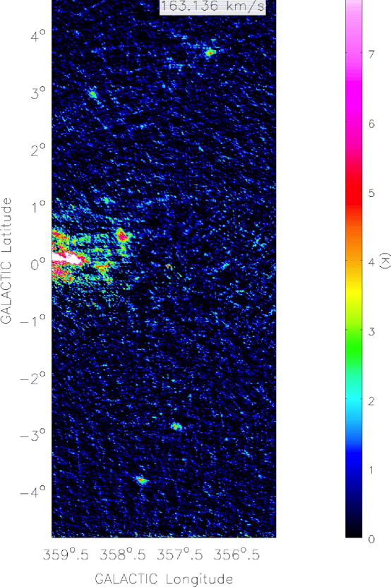
Figure 22: Examples of compact, forbidden velocity clouds at $v=163~{}{\rm km~{}s^{-1}}$ observed high above the Galactic plane. The color scale goes from $0-8$ K with a scaling power of $-0.6$, as shown in the wedge at the right. These four clouds at: $(l,b)=(358.2\arcdeg,-3.8\arcdeg)$, $(l,b)=(357.5\arcdeg,-2.9\arcdeg)$, $(l,b)=(357.0\arcdeg,+3.7\arcdeg)$ and $(l,b)=(359.0\arcdeg,+2.9\arcdeg)$ are representative examples out of the approximately 60 clouds detected in the survey area.

Figure 22 is a velocity channel image at $v=163$ ${\rm km~{}s^{-1}}$ showing several very small cloud-like features lying at high Galactic latitudes. Clouds like these are apparent throughout the cube at high ($|v|>130$ ${\rm km~{}s^{-1}}$) velocities, as well as at lower velocities where they are quite distinct from the emission related to large-scale Galactic structure, such as a tilted disk (e.g. Liszt & Burton, 1980). We find over 60 separate compact clouds in the survey area at velocities $|v|>80$ ${\rm km~{}s^{-1}}$. The properties of the detected clouds vary but typical angular sizes are $0.1-0.5$ deg, with a few larger clouds. Most of the detected clouds are faint, with brightness temperatures of $\sim 3-10$ K. Several clouds have very narrow velocity linewidths ($\sim 2$ ${\rm km~{}s^{-1}}$), but most have linewidths in the range $7-20$ ${\rm km~{}s^{-1}}$. Rough mass estimates assuming optically thin emission and a distance of 8.4 kpc (Reid et al., 2009) are in the range $250-1500~{}{\rm M_{\odot}}$. In terms of physical properties these clouds are very similar to those found by Ford et al. (2010) towards inner Galaxy tangent points.

In addition to the compact discrete clouds, there are cohesive structures like that shown in Figure 4c (bottom two panels), which forms an extended loop at $l\sim 359\arcdeg$, $b\sim-3.5\arcdeg$ pointing back towards the Galactic Center with narrow linewidth clumps along it. These high velocity features are discussed further in McClure-Griffiths et al (2012, in prep) where we elaborate on the distribution and properties of the clouds and consider the possibility that they are associated with gas entrained in a Galactic outflow (e.g. Fujita et al., 2009).

A well studied large-scale feature of the Galactic Center is the so-called Galactic Center lobe (Sofue & Handa, 1984; Law, 2010), which is traced in radio continuum, H$\alpha$, and infrared emission extending more than a degree above the plane. There is no obvious H i signature of the Galactic Center lobe. This is not surprising, however, given that the hydrogen recombination lines are at very low LSR velocities of $\sim-5$ ${\rm km~{}s^{-1}}$ to $\sim 8$ ${\rm km~{}s^{-1}}$ (Law et al., 2009), which are very crowded with H i emission. The magnetic Loop 1 of molecular gas proposed by Fukui et al. (2006), however, is easily visible in the bottom panels of Figure 4b at $v\sim-130$ ${\rm km~{}s^{-1}}$. The other loop proposed by same authors is less obvious in H i.

6 Summary

The ATCA H i survey of the Galactic Center covers the inner $10^{\circ}\times 10^{\circ}$ of the Milky Way, providing a new resource for high-angular resolution surveys of the structure and dynamics of neutral gas in the central 3 kiloparsecs of the Milky Way. We present the final H i data cube with an angular resolution of $145\arcsec$ and a velocity resolution of 1 ${\rm km~{}s^{-1}}$. The mean rms $T_{b}$ across the full area is $\sim 0.7$ K, varying from $0.5$ K to $2.0$ K, with the highest noise towards $(l,b)=0\arcdeg,0\arcdeg$.

This survey completes the International Galactic Plane Survey (McClure-Griffiths et al., 2005; Stil et al., 2006; Taylor et al., 2003) H i survey of the inner Milky Way, providing the link between the first and fourth Galactic quadrants. The data will be valuable for comparison with existing high angular resolution surveys of Galactic Center at all wavelengths. Comparison with CO (Dame et al., 2001; Oka et al., 1998) and infrared data (Molinari et al., 2011; Arendt et al., 2008) will help improve models of the inner Galaxy structure, while comparison with radio continuum and high energy emission may reveal the nature of the outflowing gas. Here we have discussed briefly some of the more noteworthy features including the near and far 3-kpc arms, a wide linewidth molecular cloud (Bania’s Clump 2) and small high velocity clumps.

Figure 1: U-V coverage of a typical pointing in the mosaic.

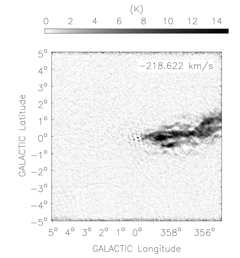
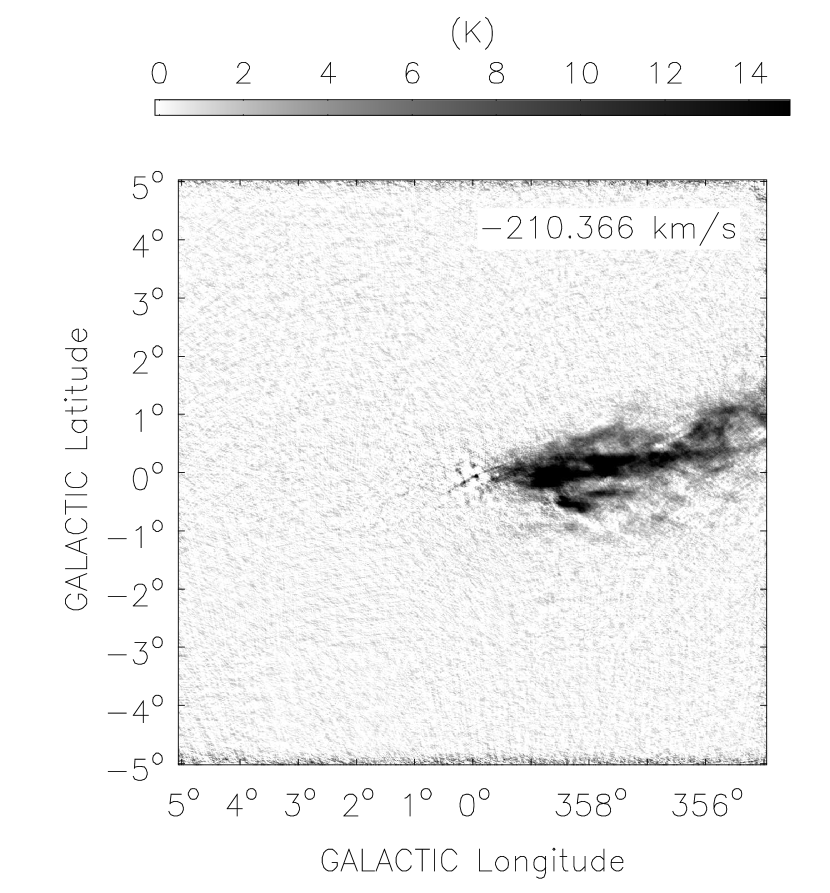
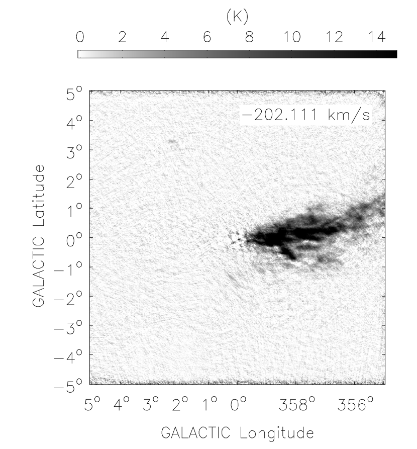
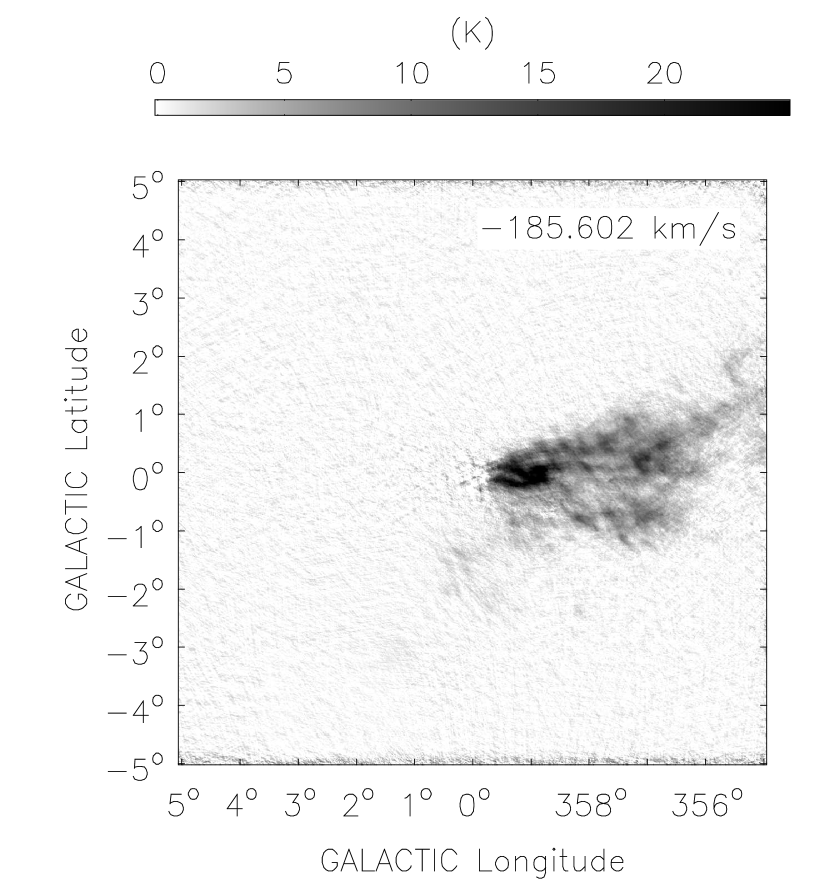
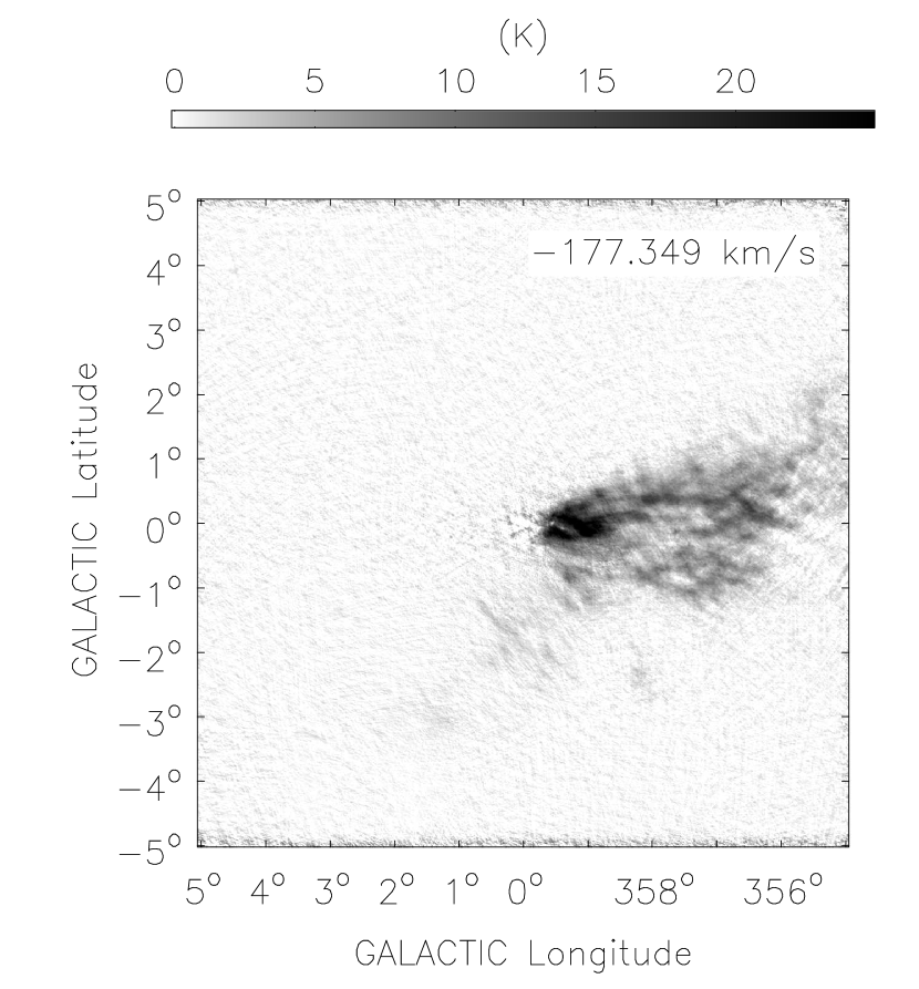
Figure 4: Velocity channel images of the full survey area. Images of every tenth channel are shown, such that the velocity spacing between images is $\sim 8$ ${\rm km~{}s^{-1}}$. The greyscale is different for each panel, as shown in the wedges above, where black is bright and white is zero or negative. These images use a scaling power of -0.6.

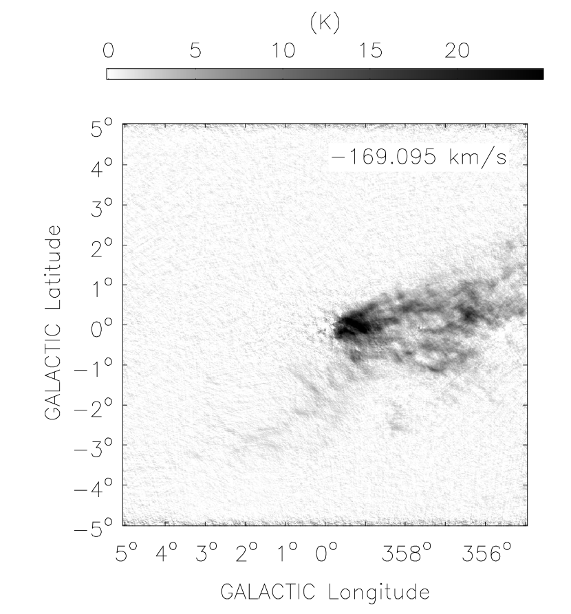
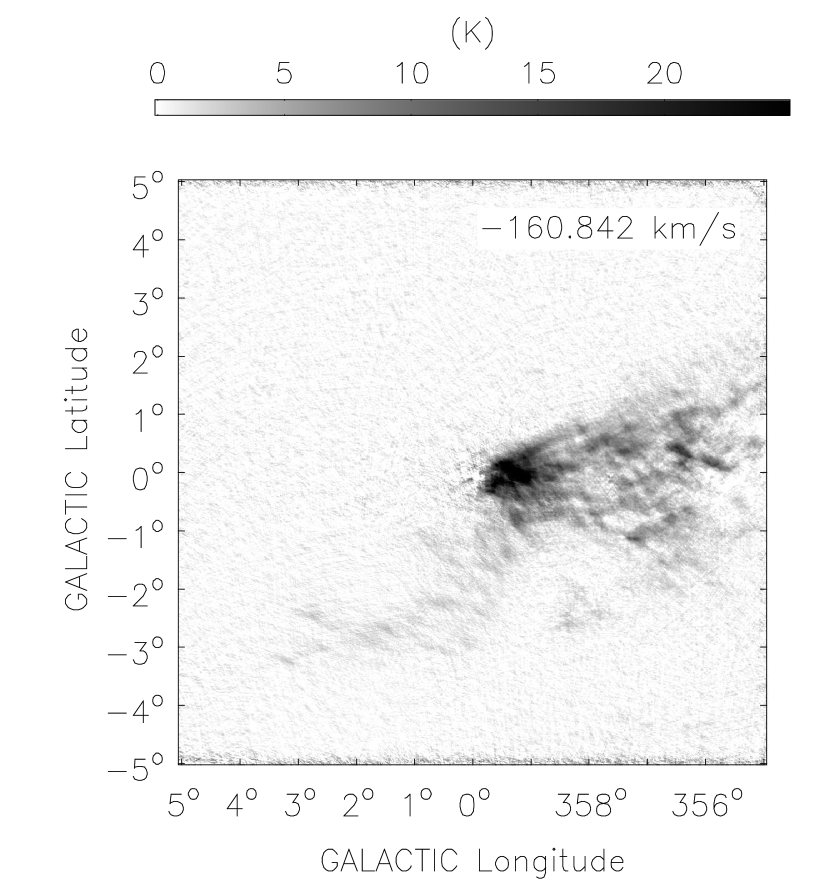
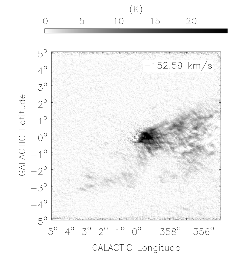
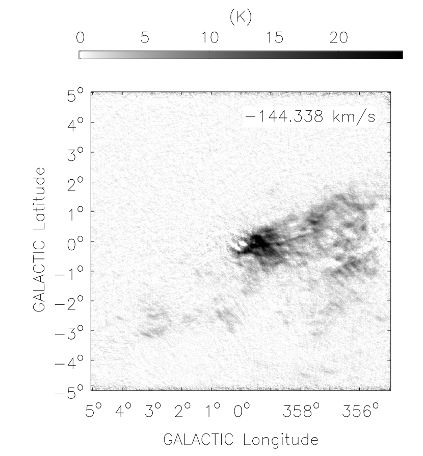
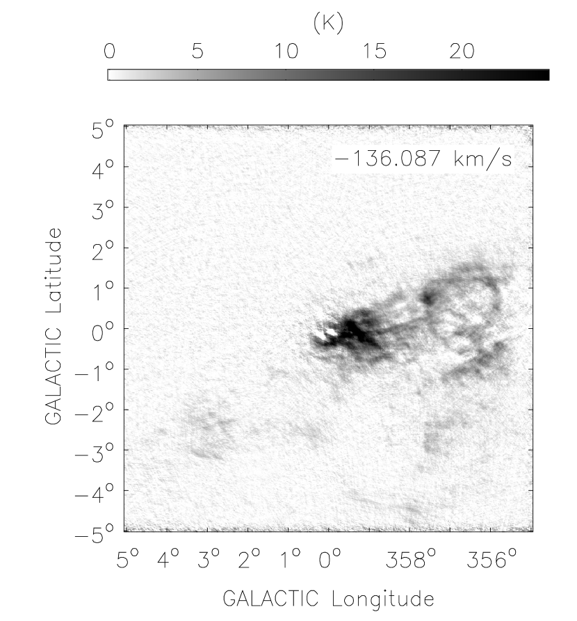
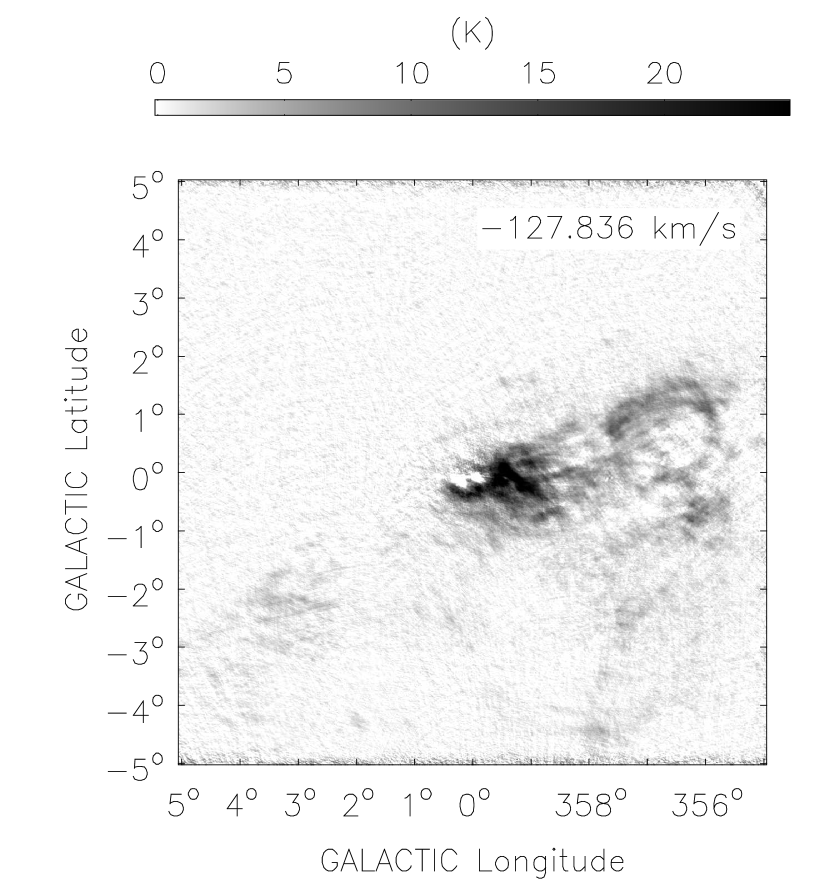
Figure 4b:

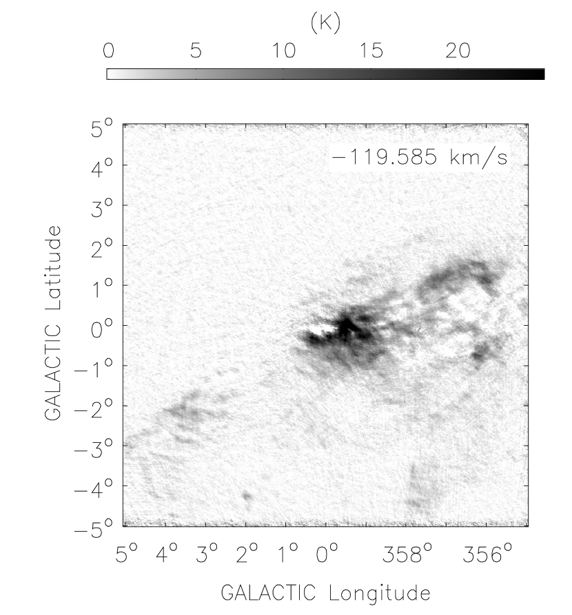
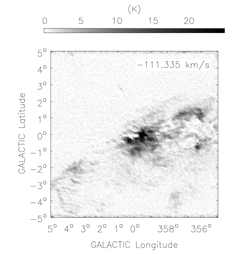
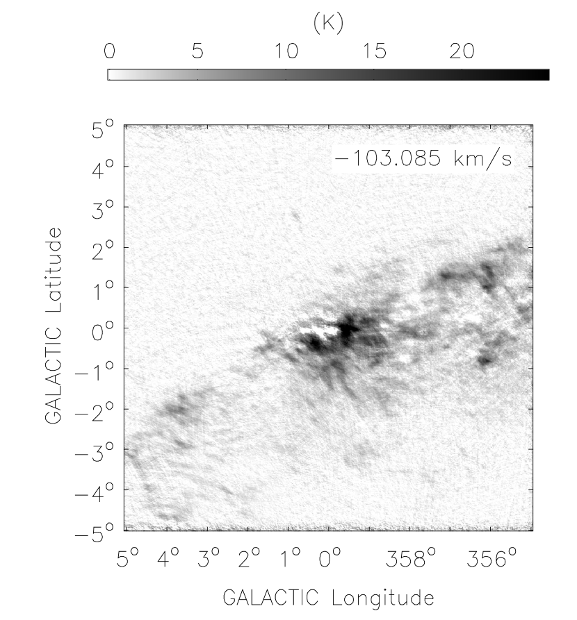
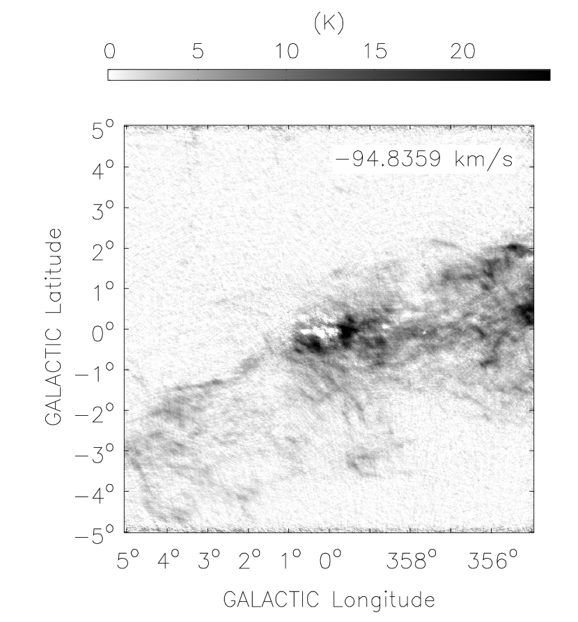
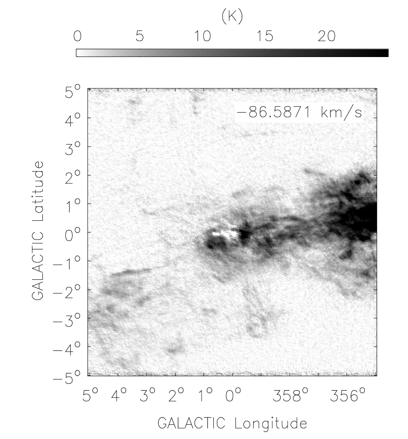
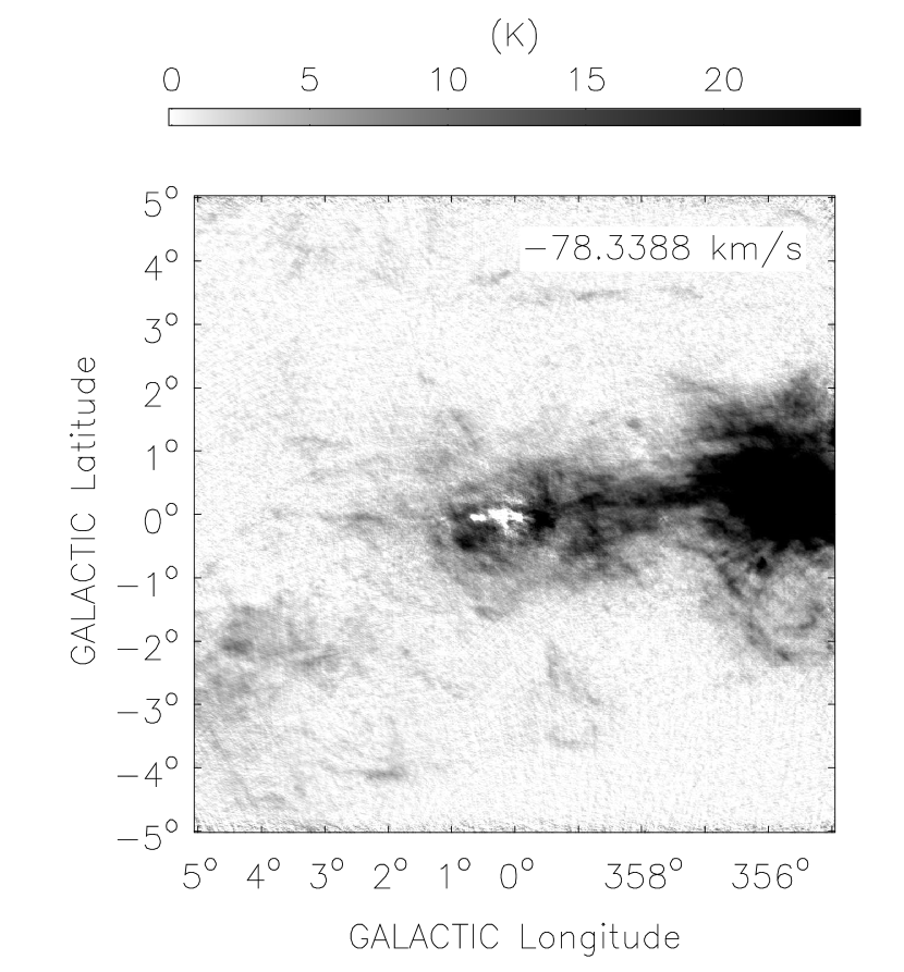
Figure 4c:

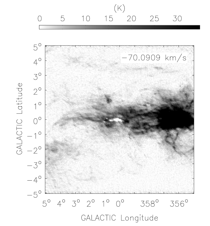
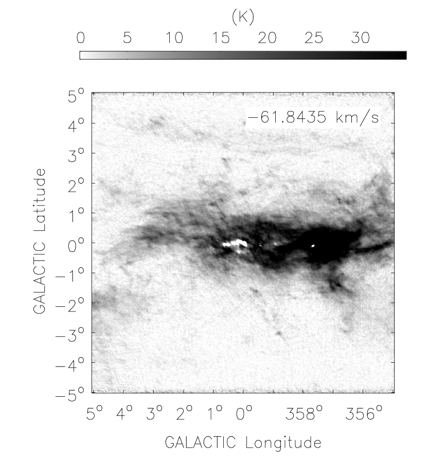
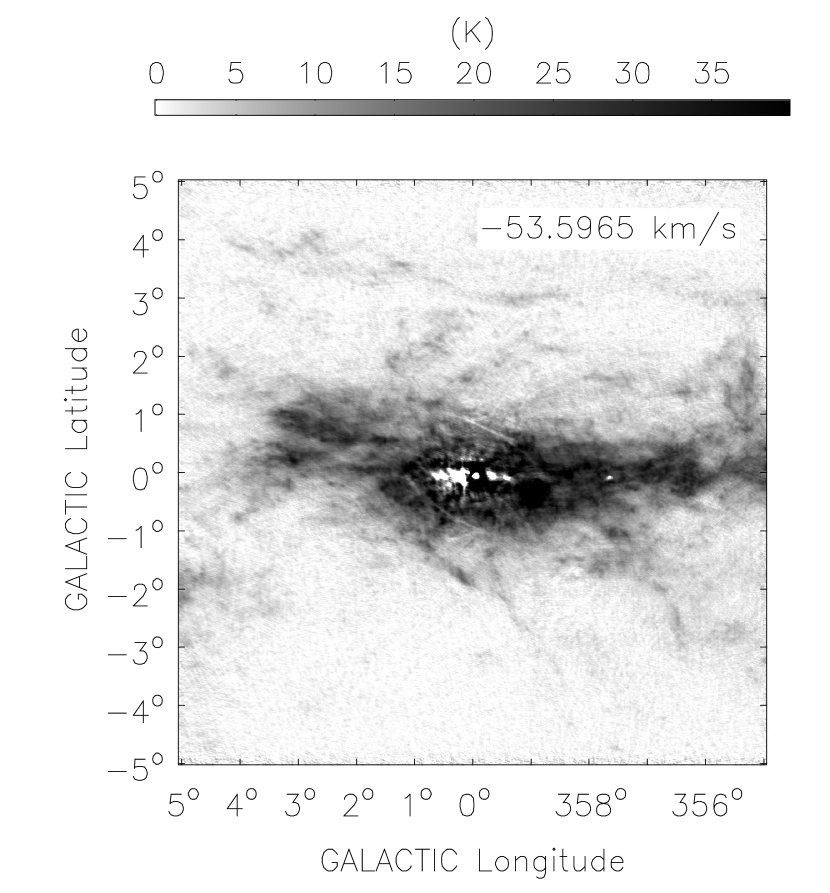
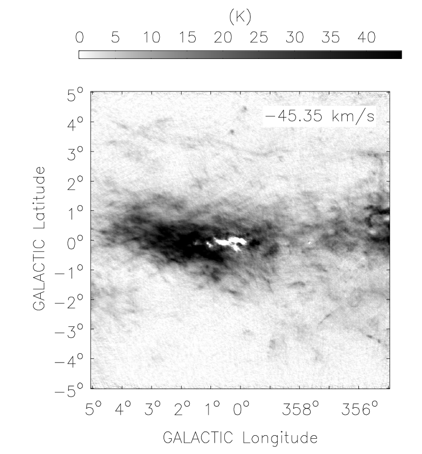
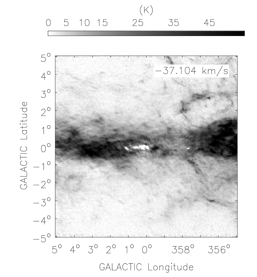
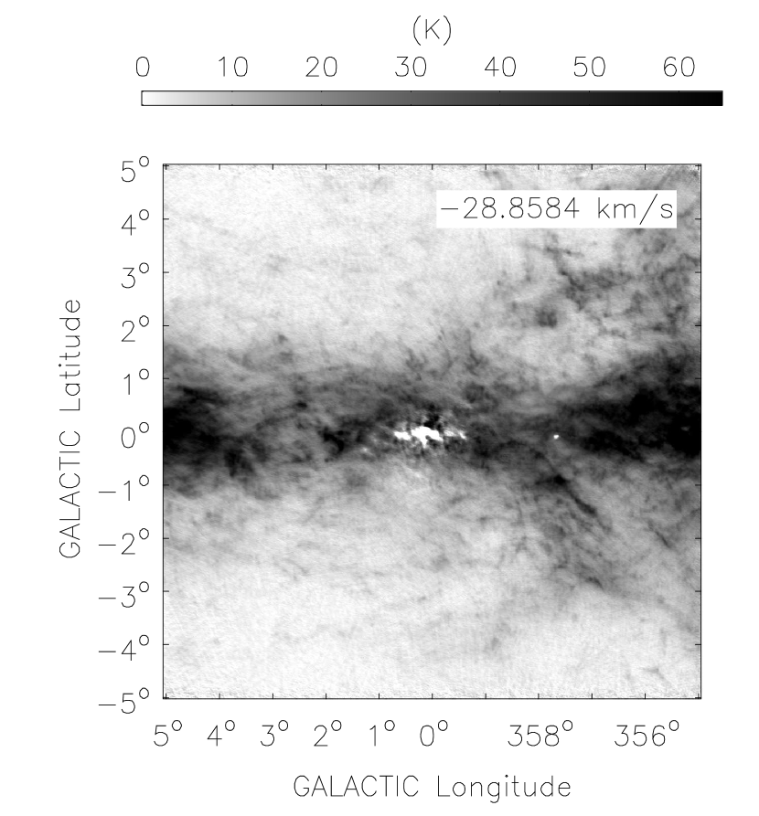
Figure 4d:

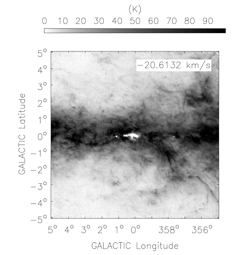
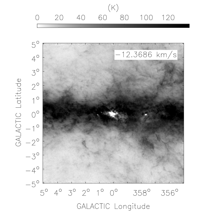
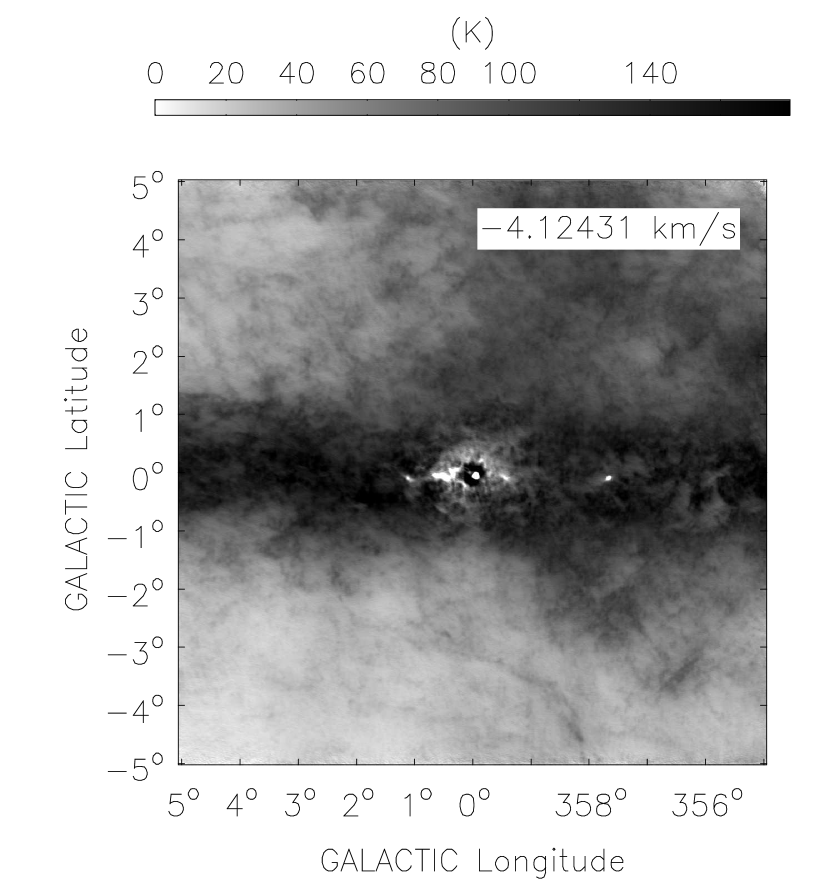
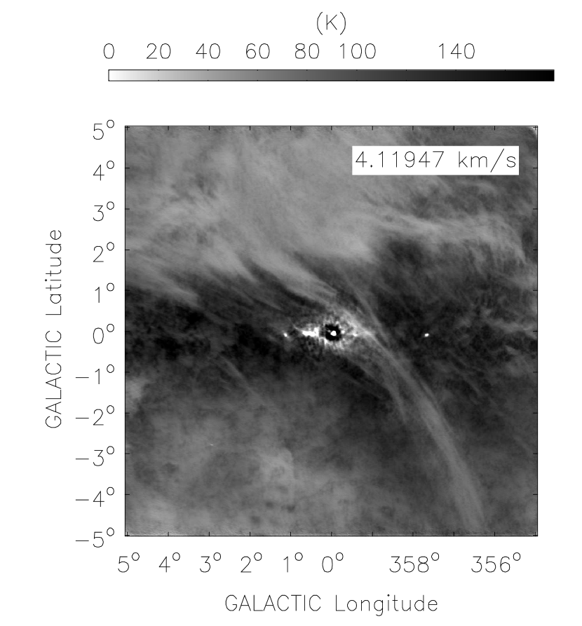
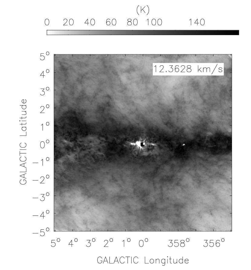
Figure 4e:

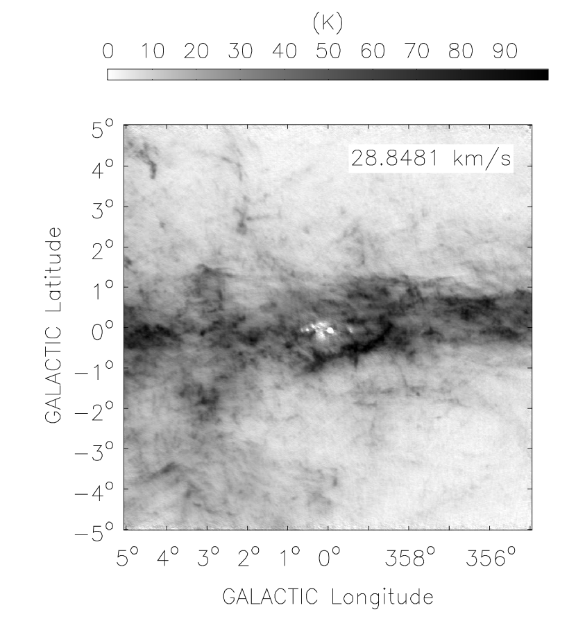
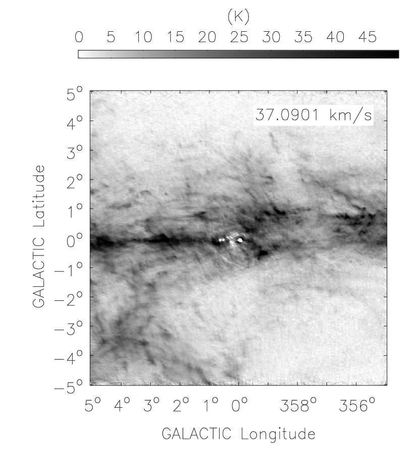
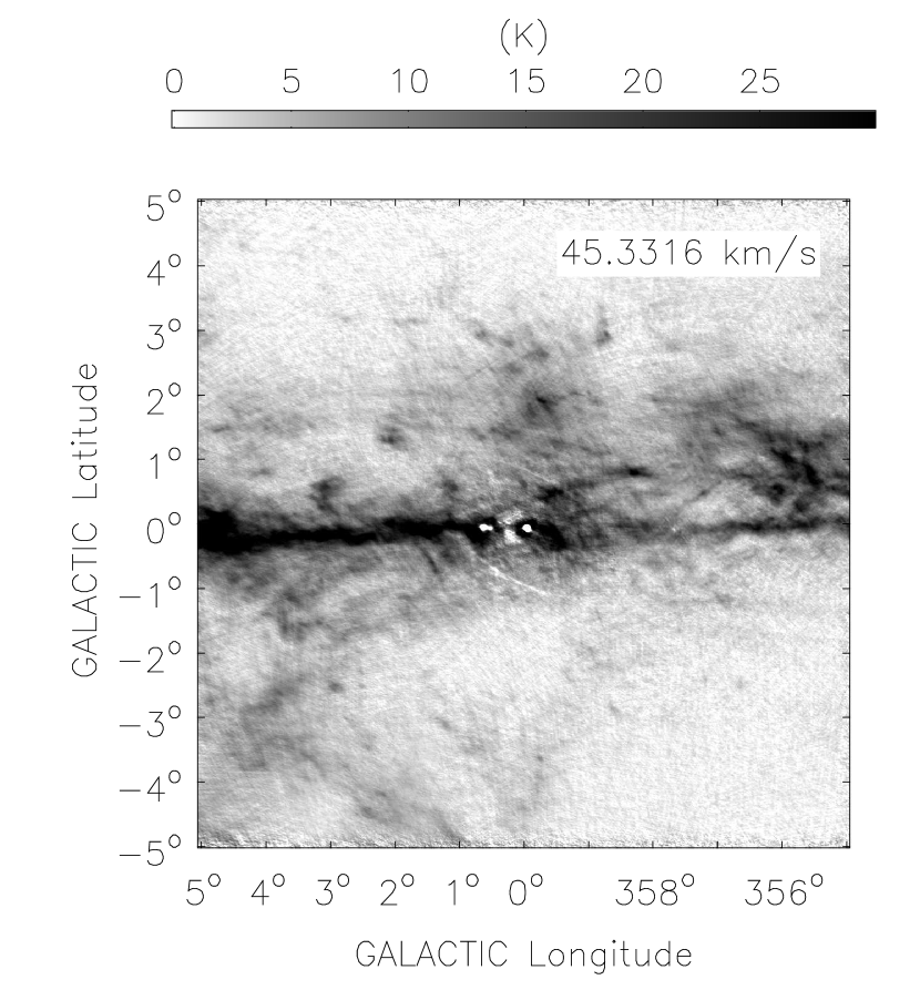
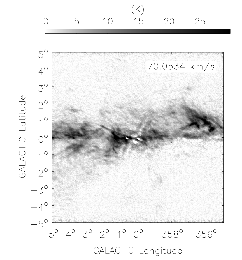
Figure 4f:

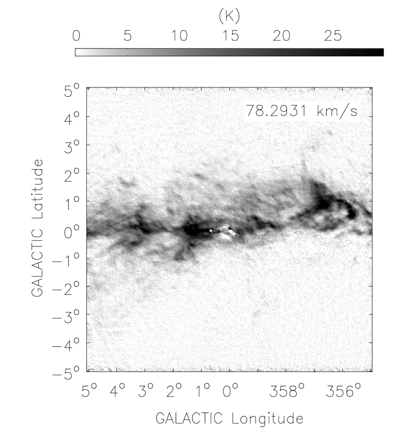
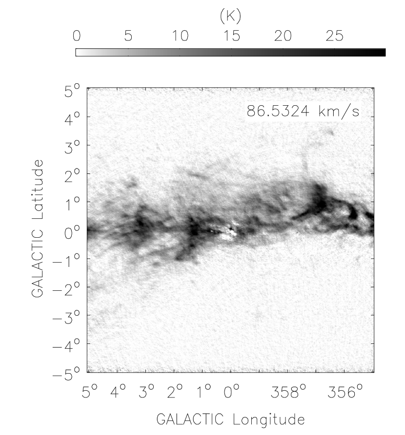
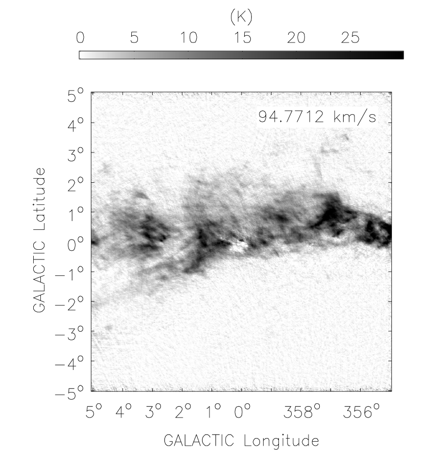
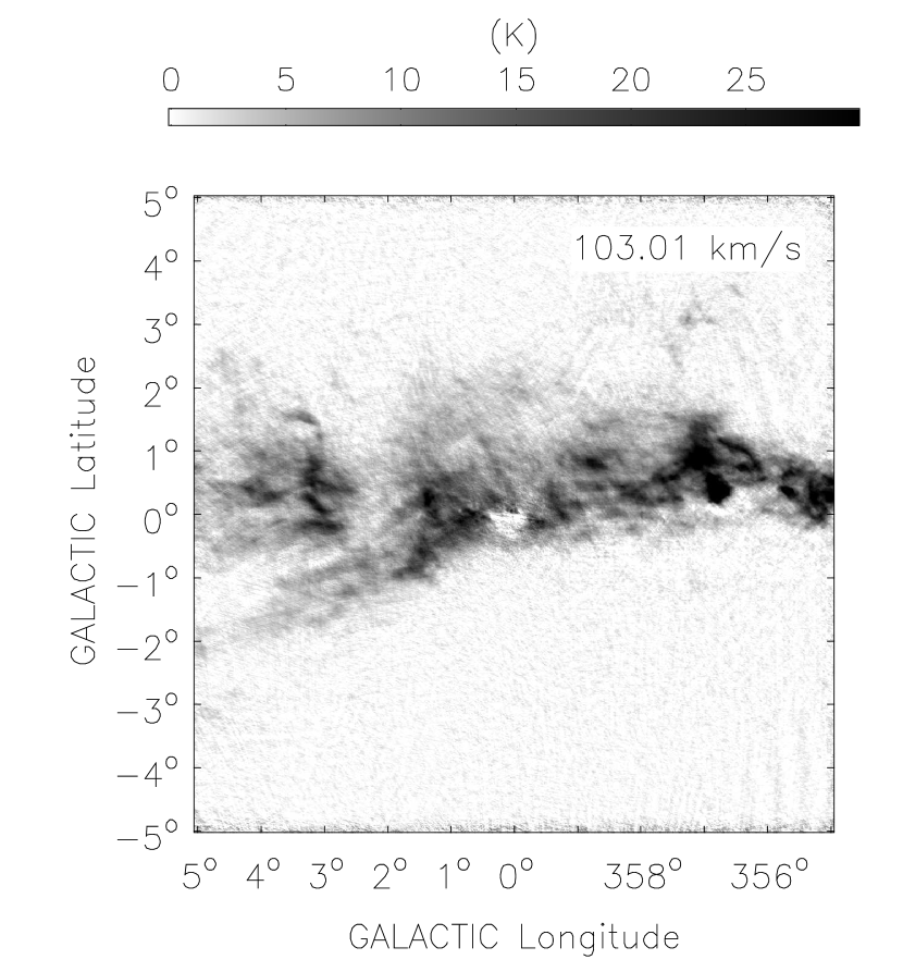
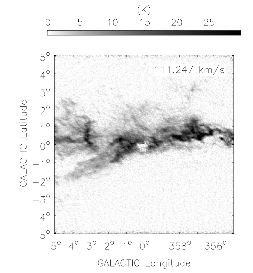
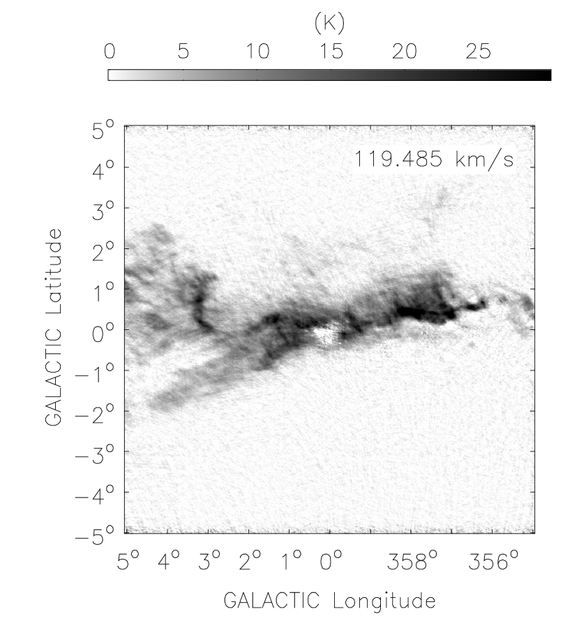
Figure 4g:

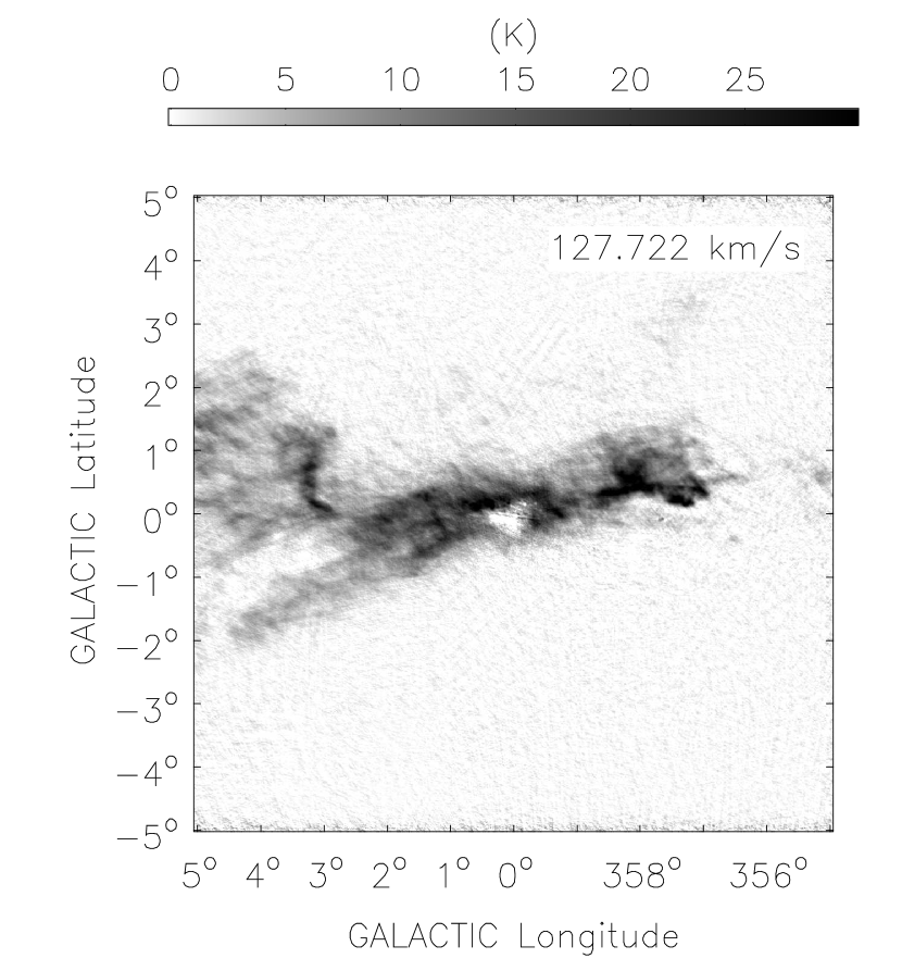
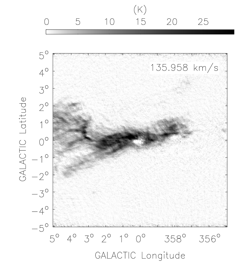
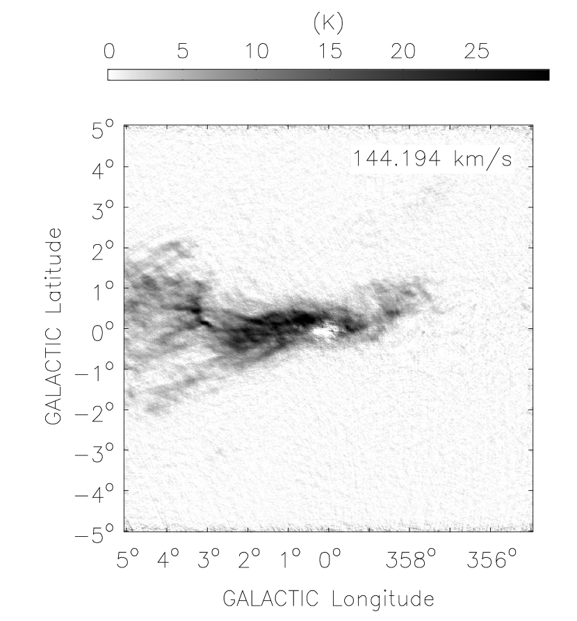
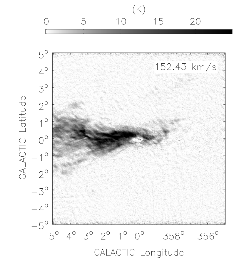
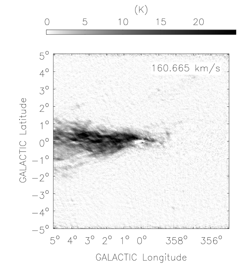
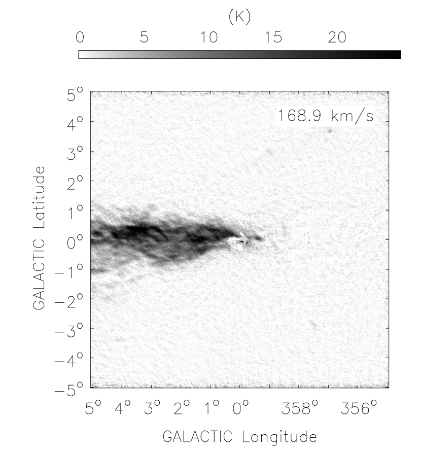
Figure 4h:

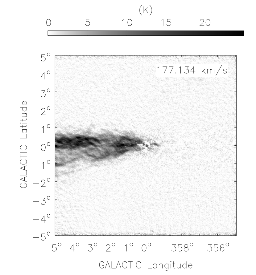
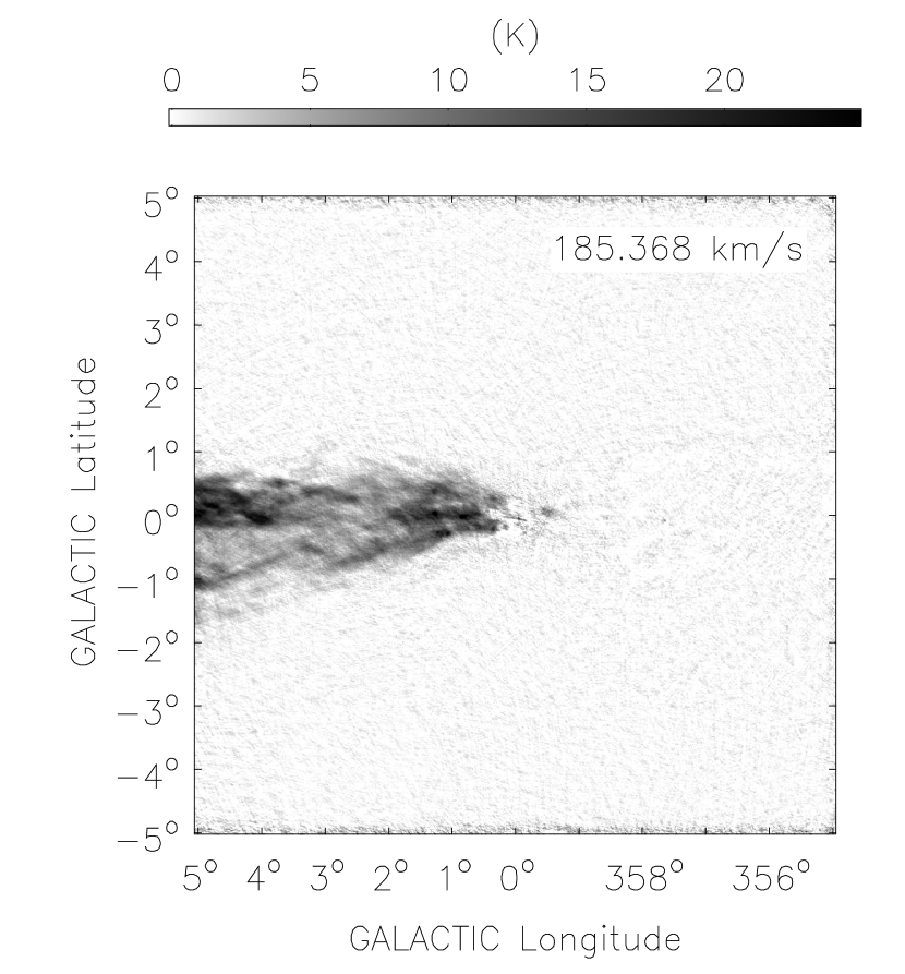
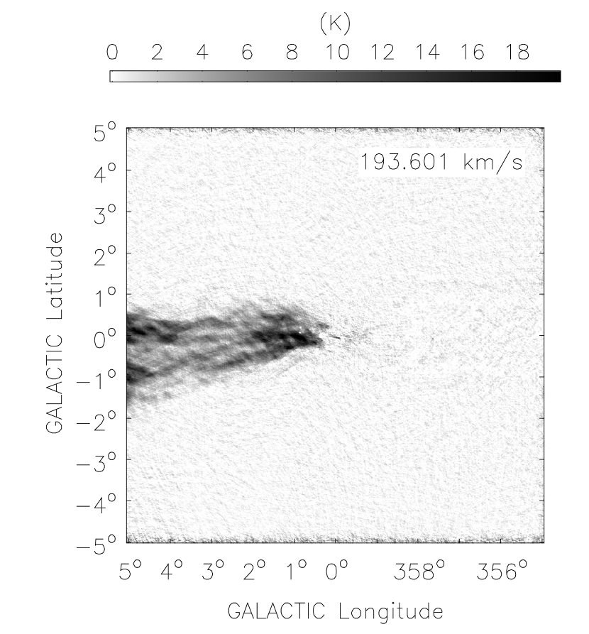
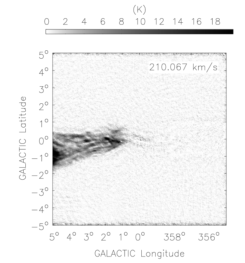
Figure 4i:

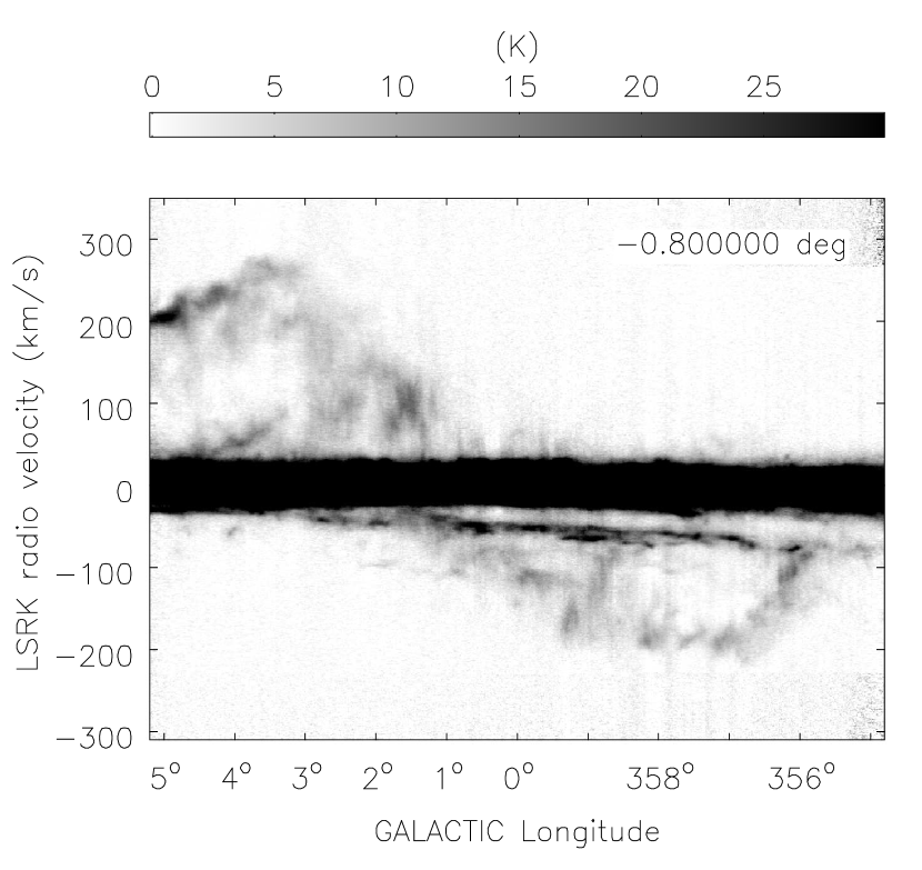
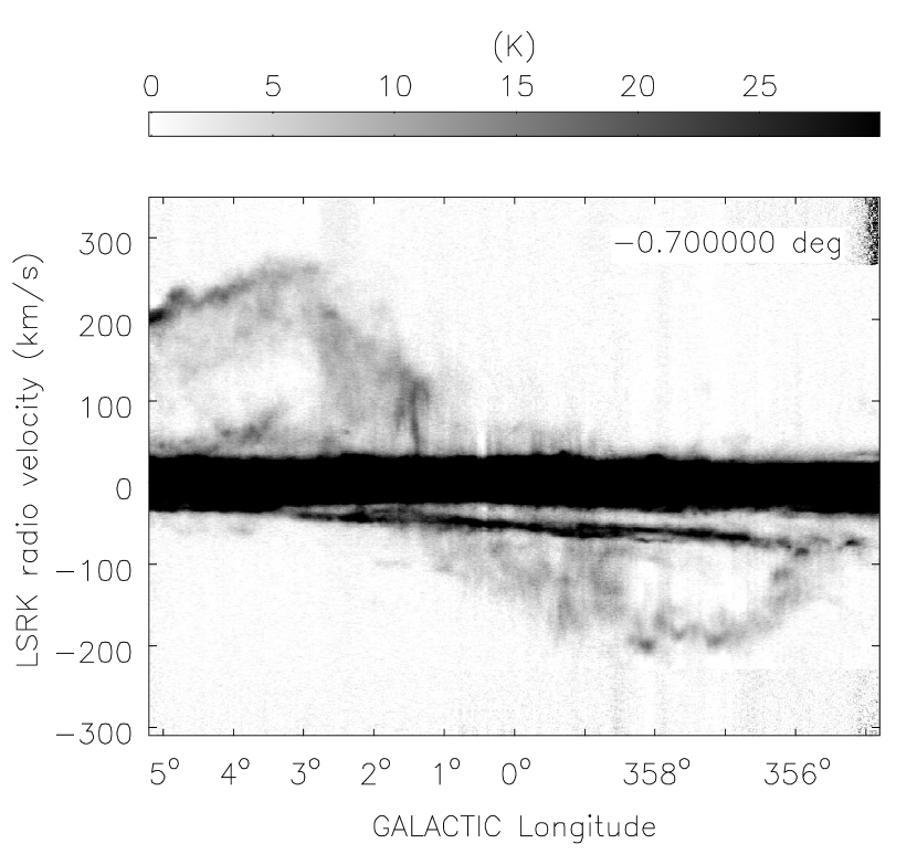
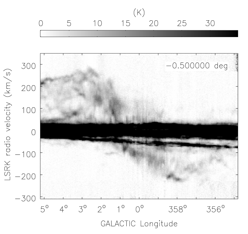
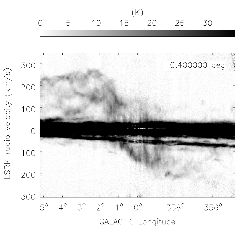
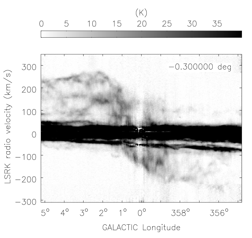
Figure 5b:

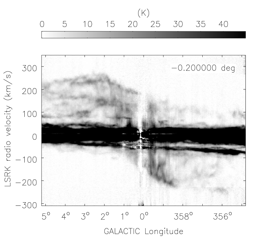
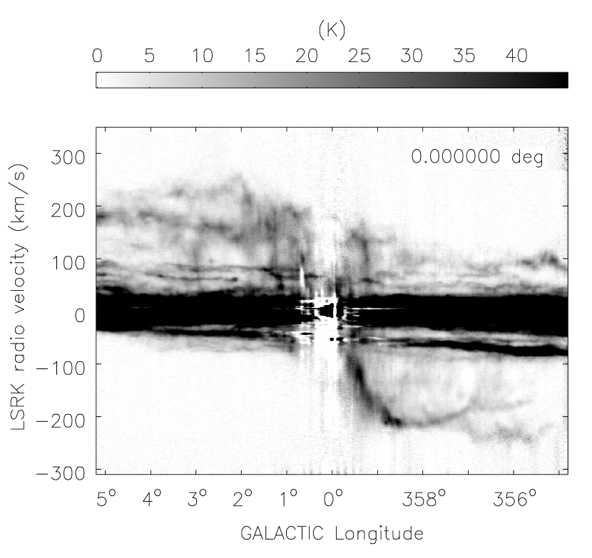
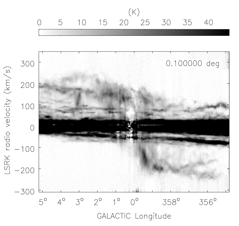
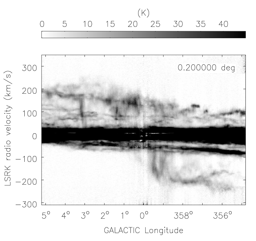
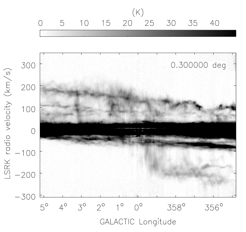
Figure 5c:

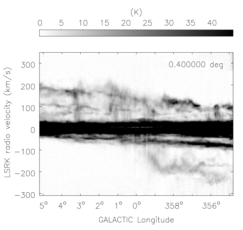
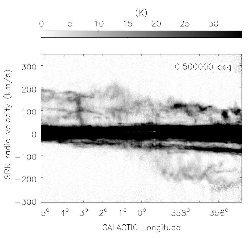
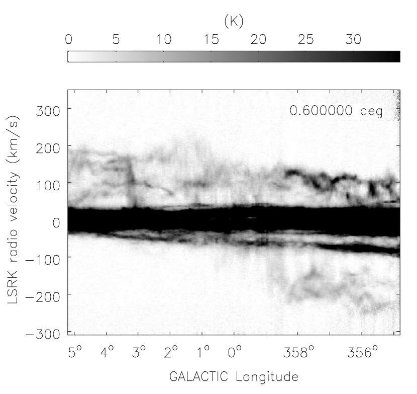
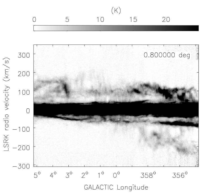
Figure 5d:

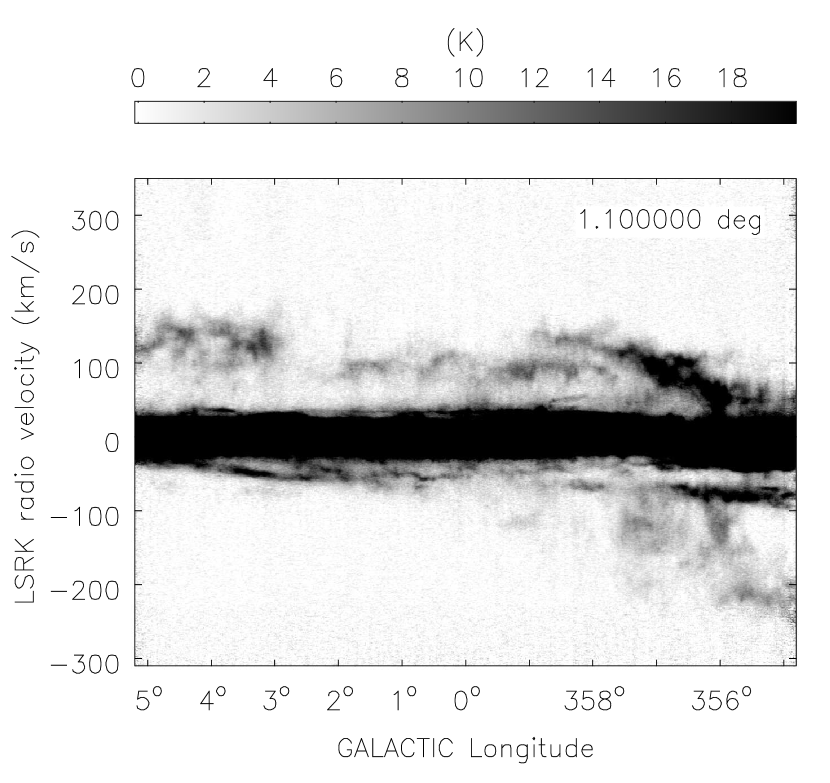
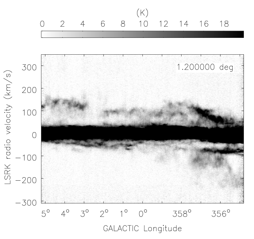
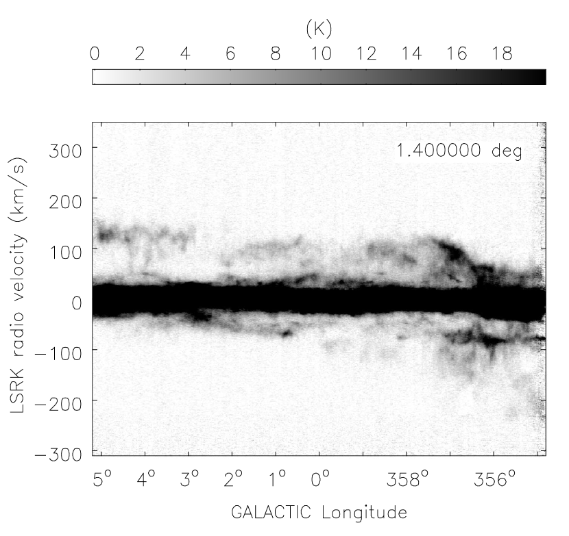
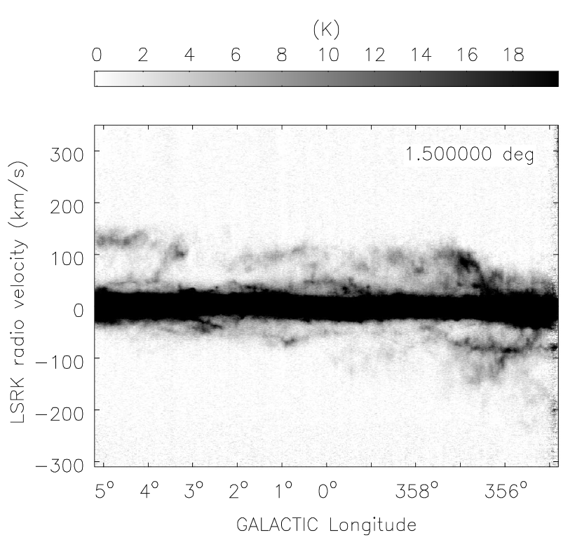
Figure 5e:

Figure 21: Slices in longitude (latitude) across the Bania’s Clump 2, showing its steep interior sides. Top: Slice at $b=0.69\arcdeg$, $v=122.78$ ${\rm km~{}s^{-1}}$. Bottom: Slice at $l=3.03\arcdeg$, $v=143.37$ ${\rm km~{}s^{-1}}$.

References

- Arendt et al. (2008) Arendt, R. G., Stolovy, S. R., Ramírez, S. V., et al. 2008, ApJ, 682, 384
- Babusiaux & Gilmore (2005) Babusiaux, C., & Gilmore, G. 2005, MNRAS, 358, 1309
- Bally et al. (2010) Bally, J., Aguirre, J., Battersby, C., & et al. 2010, ApJ, 721, 137
- Bally et al. (1987) Bally, J., Stark, A. A., Wilson, R. W., & Henkel, C. 1987, ApJS, 65, 13
- Bania (1977) Bania, T. M. 1977, ApJ, 216, 381
- Bania et al. (1986) Bania, T. M., Stark, A. A., & Heiligman, G. M. 1986, ApJ, 307, 350
- Benjamin et al. (2005) Benjamin, R. A., Churchwell, E., Babler, B. L., et al. 2005, ApJ, 630, L149
- Binney et al. (1991) Binney, J., Gerhard, O. E., Stark, A. A., Bally, J., & Uchida, K. I. 1991, MNRAS, 252, 210
- Bitran et al. (1997) Bitran, M., Alvarez, H., Bronfman, L., May, J., & Thaddeus, P. 1997, A&AS, 125, 99
- Bland-Hawthorn & Cohen (2003) Bland-Hawthorn, J., & Cohen, M. 2003, ApJ, 582, 246
- Blitz et al. (1993) Blitz, L., Binney, J., Lo, K. Y., Bally, J., & Ho, P. T. P. 1993, Nature, 361, 417
- Blitz & Spergel (1991) Blitz, L., & Spergel, D. N. 1991, ApJ, 370, 205
- Boyce & Cohen (1994) Boyce, P. J., & Cohen, R. J. 1994, A&AS, 107, 563
- Braunfurth & Rohlfs (1981) Braunfurth, E., & Rohlfs, K. 1981, A&AS, 44, 437
- Burton & Liszt (1978) Burton, W. B., & Liszt, H. S. 1978, ApJ, 225, 815
- Burton & Liszt (1983) Burton, W. B., & Liszt, H. S. 1983, A&AS, 52, 63
- Burton & Liszt (1992) —. 1992, A&AS, 95, 9
- Cabrera-Lavers et al. (2008) Cabrera-Lavers, A., González-Fernández, C., Garzón, F., Hammersley, P. L., & López-Corredoira, M. 2008, A&A, 491, 781
- Cohen (1975) Cohen, R. 1975, MNRAS, 171, 659
- Cornwell (2008) Cornwell, T. J. 2008, ISTSP, 2, 793
- Dame et al. (2001) Dame, T. M., Hartmann, D., & Thaddeus, P. 2001, ApJ, 547, 792
- Dame & Thaddeus (2008) Dame, T. M., & Thaddeus, P. 2008, ApJ, 683, L143
- Dwek et al. (1995) Dwek, E., Arendt, R. G., Hauser, M. G., et al. 1995, ApJ, 445, 716
- Ferrière et al. (2007) Ferrière, K. M., Gillard, W., & Jean, P. 2007, A&A, 467, 611
- Ford et al. (2010) Ford, H. A., Lockman, F. J., & McClure-Griffiths, N. M. 2010, ApJ, 722, 367
- Fujita et al. (2009) Fujita, A., Martin, C. L., Low, M.-M. M., New, K. C. B., & Weaver, R. 2009, ApJ, 698, 693
- Fukui et al. (2006) Fukui, Y., Yamamoto, H., Fujishita, M., et al. 2006, Science, 314, 106
- Fux (1999) Fux, R. 1999, A&A, 345, 787
- Genzel et al. (1994) Genzel, R., Hollenbach, D., & Townes, C. H. 1994, RPPh, 57, 417
- Ghez et al. (2008) Ghez, A. M., Salim, S., Weinberg, N. N., et al. 2008, ApJ, 0808, 1044
- Green et al. (2009) Green, J. A., McClure-Griffiths, N. M., Caswell, J. L., et al. 2009, ApJ, 696, L156
- Hammersley et al. (2000) Hammersley, P. L., Garzón, F., Mahoney, T. J., López-Corredoira, M., & Torres, M. A. P. 2000, MNRAS, 317, L45
- Högbom (1974) Högbom, J. A. 1974, A&AS, 15, 417
- Huettemeister et al. (1998) Huettemeister, S., Dahmen, G., Mauersberger, R., et al. 1998, A&A, 334, 646
- Kalberla et al. (2005) Kalberla, P. M. W., Burton, W. B., Hartmann, D., et al. 2005, A&A, 440, 775
- Kalberla et al. (2010) Kalberla, P. M. W., McClure-Griffiths, N. M., Pisano, D. J., et al. 2010, A&A, 521, 17
- Kerr (1967) Kerr, F. J. 1967, in IAU Symposium 31: Radio Astronomy and the Galactic System, ed. H. van Woerden, 239
- Lang et al. (2010) Lang, C. C., Goss, W. M., Cyganowski, C., & Clubb, K. I. 2010, ApJS, 191, 275
- Law (2010) Law, C. J. 2010, The Astrophysical Journal, 708, 474
- Law et al. (2009) Law, C. J., Backer, D., Yusef-Zadeh, F., & Maddalena, R. 2009, ApJ, 695, 1070
- Lee (1996) Lee, C. W. 1996, ApJS, 105, 129
- Liszt (2006) Liszt, H. S. 2006, A&A, 447, 533
- Liszt (2008) —. 2008, A&A, 486, 467
- Liszt & Burton (1978) Liszt, H. S., & Burton, W. B. 1978, ApJ, 226, 790
- Liszt & Burton (1980) —. 1980, ApJ, 236, 779
- Martin et al. (2004) Martin, C. L., Walsh, W. M., Xiao, K., et al. 2004, ApJS, 150, 239
- McClure-Griffiths et al. (2003) McClure-Griffiths, N. M., Dickey, J. M., Gaensler, B. M., & Green, A. J. 2003, ApJ, 594, 833
- McClure-Griffiths et al. (2005) McClure-Griffiths, N. M., Dickey, J. M., Gaensler, B. M., et al. 2005, ApJS, 158, 178
- McClure-Griffiths et al. (2009) McClure-Griffiths, N. M., Pisano, D. J., Calabretta, M. R., et al. 2009, ApJS, 181, 398
- Molinari et al. (2011) Molinari, S., Bally, J., Noriega-Crespo, A., & et al. 2011, ApJ, 735, L33
- Molinari et al. (2010) Molinari, S., Swinyard, B., Bally, J., & et al. 2010, A&A, 518, L100
- Morris & Serabyn (1996) Morris, M., & Serabyn, E. 1996, ARA&A, 34, 645
- Oka et al. (1998) Oka, T., Hasegawa, T., Sato, F., Tsuboi, M., & Miyazaki, A. 1998, ApJS, 118, 455
- Oort et al. (1958) Oort, J. H., Kerr, F. J., & Westerhout, G. 1958, MNRAS, 118, 379
- Peters (1975) Peters, III, W. L. 1975, ApJ, 195, 617
- Reid et al. (2009) Reid, M. J., Menten, K. M., Zheng, X. W., et al. 2009, ApJ, 700, 137
- Reynolds (1994) Reynolds, J. E. 1994, ATNF Technical Document Series, Tech. Rep. AT/39.3/0400, Australia Telescope National Facility, Sydney
- Riffert et al. (1997) Riffert, H., Kumar, P., & Huchtmeier, W. K. 1997, Monthly Notices of the Royal Astronomical Society, 284, 749
- Rodriguez-Fernandez et al. (2006) Rodriguez-Fernandez, N. J., Combes, F., Martin-Pintado, J., Wilson, T. L., & Apponi, A. 2006, A&A, 455, 963
- Romero-Gómez et al. (2011) Romero-Gómez, M., Athanassoula, E., Antoja, T., & Figueras, F. 2011, MNRAS, 418, 1176
- Sanders & Wrixon (1972) Sanders, R. H., & Wrixon, G. T. 1972, A&A, 18, 467
- Sault (1994) Sault, R. J. 1994, A&AS, 107, 55
- Sault et al. (1995) Sault, R. J., Teuben, P. J., & Wright, M. C. H. 1995, in in ASP. Conf. Ser. 77, Astronomical Data Analysis Software and Systems IV, ed. R. A. Shaw, H. E. Payne, & J. J. E. Hayes (San Francisco, CA: ASP), 433
- Sawada et al. (2004) Sawada, T., Hasegawa, T., Handa, T., & Cohen, R. J. 2004, MNRAS, 349, 1167
- Sofue & Handa (1984) Sofue, Y., & Handa, T. 1984, Nature, 310, 568
- Stanimirović (2002) Stanimirović, S. 2002, in ASP Conf. Ser. 278: Single-Dish Radio Astronomy: Techniques and Applications, ed. S. Stanimirovic, D. Altschuler, P. Goldsmith, & C. Salter (San Francisco, CA: ASP), 375
- Stark & Bania (1986) Stark, A. A., & Bania, T. M. 1986, ApJ, 306, L17
- Stil et al. (2006) Stil, J. M., Taylor, A. R., Dickey, J. M., et al. 2006, AJ, 132, 1158
- Tanaka et al. (2007) Tanaka, K., Kamegai, K., Nagai, M., & Oka, T. 2007, PASJ, 59, 323
- Taylor et al. (2003) Taylor, A. R., Gibson, S. J., Peracaula, M., et al. 2003, AJ, 125, 3145
- van der Kruit (1970) van der Kruit, P. C. 1970, A&A, 4, 462
- van der Kruit (1971) —. 1971, A&A, 13, 405
- van Woerden et al. (1957) van Woerden, H., Rougoor, G. W., & Oort, J. H. 1957, CRAS, 244, 1961
- Wilson et al. (2011) Wilson, W. E., Ferris, R., Axtens, P., & et al. 2011, MNRAS, 416, 832