Self-consistent field theory of polarized BEC: dispersion of collective excitation

Abstract

We suggest the construction of a set of the quantum hydrodynamics equations for the Bose-Einstein condensate (BEC), where atoms have the electric dipole moment. The contribution of the dipole-dipole interactions (DDI) to the Euler equation is obtained. Quantum equations for the evolution of medium polarization are derived. Developing mathematical method allows to study effect of interactions on the evolution of polarization. The developing method can be applied to various physical systems in which dynamics is affected by the DDI. Derivation of Gross-Pitaevskii equation for polarized particles from the quantum hydrodynamics is described. We showed that the Gross-Pitaevskii equation appears at condition when all dipoles have the same direction which does not change in time. Comparison of the equation of the electric dipole evolution with the equation of the magnetization evolution is described. Dispersion of the collective excitations in the dipolar BEC, either affected or not affected by the uniform external electric field, is considered using our method. We show that the evolution of polarization in the BEC leads to the formation of a novel type of the collective excitations. Detailed description of the dispersion of collective excitations is presented. We also consider the process of wave generation in the polarized BEC by means of a monoenergetic beam of neutral polarized particles. We compute the possibilities of the generation of Bogoliubov and polarization modes by the dipole beam.

I I. Introduction

After obtaining the Bose-Einstein condensate (BEC) in experiments with vapors of alkaline metal atoms, theoretical and experimental investigation of linear waves and nonlinear structures in the BEC have been performed. In recent years the interest to the polarized BEC has been increasing. It is connected with recent experimental progress in cooling of polarized atoms and molecules. At present day the BEC with magnetic polarization is realized on atoms ⁵²Cr. There are a lot of attempt of experimental obtaining of the electrically polarized BEC (see reviews  Koberle NJP 09 - Ni PCCP 09 ). For this aim, Bose molecules having the electric dipole moment have been cooled. Particular interest to the electrically polarized BEC brought because of large dipole-dipole scattering length, and thereby because of both the big magnitude and large distance of interaction in compare with analogous quantities for the magnetized BEC.

Many processes in quantum systems are determined by the dynamics and the dispersion of collective excitations (CE)  Griffin book . The law dispersion of the CE in the degenerate dilute Bose gas was obtained by Bogoliubov in 1947  Bogoliubov N.1947 ; L.P.Pitaevskii RMP 99 . Many authors studied the change of the Bogoliubov spectrum which arises when the short-range interaction accounted more carefully  Pu PRL 02 - Andreev PRA08 , or geometry of the system is complex  Stringari PRL 96 ,  Falco PRA 07 ,  mass dep of waves in BEC . In papers  Santos PRL 03 - Ticknor PRL 11 authors studied the influence of the electric dipole moment (EDM) dynamics on the dispersion of the CE in the BEC. The contribution of polarization in the dispersion law of the Bogoliubov mode was obtained in Ref.s  Santos PRL 03 - Ticknor PRL 11 . Instability of the Bogoliubov spectrum in the 3D dipolar BEC (DBEC) with the repulsive short-range interaction (SRI) was shown in Ref.s  Santos PRL 03 - Giovanazzi EPJD 04 . U. R. Fisher  Fischer PRA 06R obtained that the Bogoliubov mode in the 2D DBEC is stable for a wide range of system parameters. There are also review papers  Carr NJP 09 - Ni PCCP 09 , where various aspects of physics of the polarized BEC were considered. In this paper we are interested in possibility of the polarization wave existence in the DBEC, i.e. in existence of new type of the CE. Dynamics of polarization is interesting not for the quantum gases only, but in the solid state physics and the physics of low-dimensional systems too. The polarization waves in the low dimensional and the multy-layer systems of conductors, dielectrics, and semiconductors are considered in the papers  Andreev PRB 11 ; Qiuzi Li PRB 11 . Analogously, in the BEC of molecules having the EDM we expect the existence of a polarization wave along with the Bogoliubov mode.

For investigation of the BEC, in system of particles with the EDM or the magnetic moments, various theoretical methods are used. One of the ways of theoretical description of the polarized BEC is the generalization of well-known Gross-Pitaevskii (GP) equation  Yi PRA 00 - Goral PRA 02 . In this way next papers were made: for the spinor BEC  Szankowski PRL 10 ; Cherng PRL 09 ; Lahaye RPP 09 , for the effect of magnetic moment on the BEC evolution  Lahaye RPP 09 - Lahaye Nature and for the influence of electrical polarization of atoms on the dynamic processes in the BEC  Lahaye RPP 09 - polarized BEC first step . Dipolar fermions also attract a lot of attention  Lu 11 arxiv ,  Gadsbolle 11 arxiv .

The same generalization of the GP equation is usually used for the magnetic moments and the electric dipoles:

$$\imath\hbar\partial_{t}\Phi(\textbf{r},t)=\biggl{(}-\frac{\hbar^{2}\nabla^{2}}{2m}+\mu(\textbf{r},t)+V_{ext}(\textbf{r},t)+g\mid\Phi(\textbf{r},t)\mid^{2}$$

$$+d^{2}\int d\textbf{r}^{\prime}\frac{1-3\cos^{2}\theta^{\prime}}{|\textbf{r}-\textbf{r}^{\prime}|^{3}}\mid\Phi(\textbf{r}^{\prime},t)\mid^{2}\biggr{)}\Phi(\textbf{r},t).$$ (1)

In equation (1) following designation are used: $\Phi(\textbf{r},t)$ is the macroscopic wave function, $\mu$ is the chemical potential, $V_{ext}$ is the potential of external field, $g$ is the constant of short-range interaction, $d$ is the dipole electric moment of single atom, $m$ is the mass of particles and $\hbar$ is the Planck constant divided by $2\pi$.

Along with the GP equation the method of quantum hydrodynamics (QHD) is also used. The method of QHD  Andreev PRA08 ,  MaksimovTMP 1999 ,  Andreev arxiv 12 01 was used for investigations of various physical systems, particularly for the BEC  Andreev PRA08 ,  Andreev arxiv ThPart and the polarization waves in conductors and semiconductors  Andreev PRB 11 . Therefore, the method of QHD could be used to consider the possibility of arising polarization waves in the BEC and calculate of the dispersion law of these waves.

At interpretation of the DDI in the quantum gases (QG) used the notion of the scattering length (SL) and the first Born approximation (FBA), analogously to the SRI described by the fourth term in the right-hand side of equation (1). Therefore, the problem reduces to the process of scattering. Different approximations based on scattering process was analyzed in Ref.  Wang NJP 08 . Particularly, where were considered condition of the FBA using and presented generalization of the GP equation for the scattering of polarized atoms beyond the FBA.

Considering the QHD we do not formulate the scattering problem. We do not need to limit ourselves to a scattering process, because we are interested in interaction between atoms including interaction between several atoms at the same time. This statement is especially important for the polarized atoms because of the long-range interaction between dipoles. Each act of interaction between dipoles could be considered as the scattering process for system of particles with a low concentration. This approximation is possible as for the neutral polarized particles as for the charged particles. The kinetic theory for the last case was developed by L. D. Landau in 1936  Landau v10 . Landau constructed collision term for the Coulomb particles, using analogy with the Boltzmann equation. The Landau collision integral depends on a scattering cross section. In this connection he considered the problem of the scattering of charged particles on small angles, that is suitable for rare systems. Strictly speaking, for particles with the long-range interaction the conception of the self-consistent field is more suitable. This conception was suggested by A. A. Vlasov in 1938, for system of the charged particles  Vlasov JETP 38 . In fact, group of particles moves in the field of their neighbors, but state of motion of the neighbors depends on motion of this group of particles as well (This picture of interaction is described on Fig. 1). According to this idea Vlasov proposed a kinetic equation for the charged particles called the Vlasov equation. Actually the Landau collision integral and the Vlasov equation are the two opposite branches of a hypothetical general theory. In this paper we follow to the Vlasov approximation and derive the self-consistent field theory for the dipole-dipole interaction in the quantum gases. From this point of view, there is no need to consider the first Born approximation or scattering process. In Appendix B to this paper we present derivation of the GP equation for polarized particles from the QHD equations. We did it at the condition that dipoles are parallel each other and to an external field, they directions do not oscillate or vibrate around an equilibrium direction.

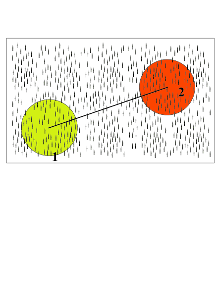
Figure 1: (Color online) The figure presents the picture of the self-consistent interaction between dipoles. Total polarization of region 2 (red) interacts with total polarization of region 1 (green). Changing the extreme point of a radius vector (or shifting the region 2) we can scan whole space. In this way we obtain action of external dipoles on region 1. Changing position of region 1 and repeating described operation we obtain action of surrounding dipoles on each region of space. This is a picture of the self-consistent interaction in fixed moment of time and this picture governs an evolution of polarization in system. This picture of interaction is typical for the classic physics, where we need to obtain smooth functions describing collective motion. For this aim is necessary to average the collective variables at the physically infinitesimal volume (sketched circle). In quantum mechanics, where the particle concentration, polarization of medium, etc, are defined via wave function and we can consider described picture on interaction of separate particle instead of space regions.

Other methods were also applied for investigation of the polarized BEC and other systems of particles having the EDM, along with the GP equation. A hydrodynamic formulation of the Hartree-Fock theory for particles with the significant EDM is considered in Ref.  Lima PRA 10 . The Euler-type equation was derived in paper  Lima PRA 10 , from the evolution of the density matrix. The EDM dynamics in dimer Mott insulators causes the rise of the low-frequency mode  Gomi PRB 10 . The spectrum of single-particle excitations and long-wave-length collective modes (zero sound) in the normal phase were obtained  Sieberer PRA 11 in the Hartree-Fock approximation, which treats direct and exchange interactions on an equal footing. Minimal coupling model for description of spatial polarization changing on the BEC properties is constructed in Ref.  Wilson arxiv 11 . The density functional method was used for the polarized quantum gas studying in Ref.  Fang PRA 11 . The Hubbard model for the polarized BEC is used too  He PRA 11 . A two-body quantum problem for the polarized molecules is analyzed in  Quemener PRA 11 . The existence of states with spontaneous interlayer coherence has been predicted in  Lutchyn PRA 10 in systems of the polar molecules. Calculations, in  Lutchyn PRA 10 , were based upon the secondary quantization approach, where the Hamiltonian accounts for the molecular rotation and the dipole-dipole interactions. Superfluidity anisotropy of polarized fermion systems was shown in  Liao PRA 10 and their thermodynamic and correlation properties were investigated  Baillie PRA 10 . The effect of the EDM on a system of cooled neutral atoms which are used for the quantum computing and quantum memory devices was analyzed in Ref.  Gillen-Christandl PRA 11 .

The characteristic property of the BEC in a system of excitons inducing in semiconductors  Deng RMP 10 is a significant value of the exciton EDM. This leads to strong interaction of excitons with an external electric field and emergence of the collective DDI in exciton systems. The QHD method may be applied to such systems along with quantum kinetics based on the nonequilibrium Green functions  Haug book 08 or the density matrix equations  Kuhn book 97 .

Notable success has been reached in the Bose condensation of dense gases  Vogl Nature 09 ; Sheik-Bahae NP 09 . Consequently, we need the detailed account of the short range interaction for investigation of the EDM dynamics. In this work we account the SRI up to the third order on interaction radius (TOIR)  Andreev PRA08 . This approximation leads to nonlocality of the SRI  Andreev PRA08 ,  Rosanov PL A 02 - Andreev arxiv 11 1 .

Electrically polarized BEC can interact with the beam of charged and polarized particles by means of the charge-dipole and the dipole-dipole interaction. These interactions lead to transfer of energy from the beam to medium and, consequently, to generation of waves. In the plasma physics, the effects of generation of waves by electron  Bret PRE 04 or magnetized neutron  Andreev PIERS 2011 ; Andreev arxiv MM beam are well-known. When we use term beam we also mean stream of particles excited in the considered system, along with an external beam of particles passing through the system. In presented paper we consider similar effect in the polarized BEC.

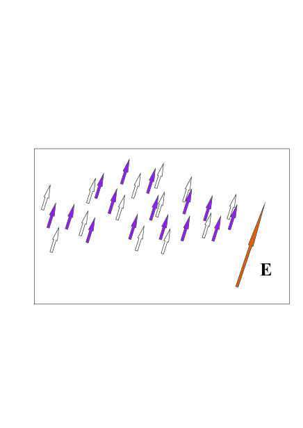
Figure 2: (Color online) The figure shows motion of dipoles without changing of direction of dipoles during motion. Dipoles stand at temperature equal to zero $T=0$ and in external uniform static electric field E. This picture describes particles in two different moments of time. White dipoles presents system in the first moment of time, and violet dipoles are present system in the next moment.

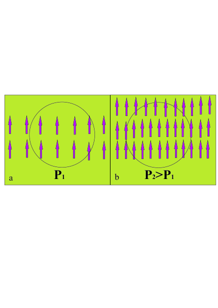
Figure 3: (Color online) The figure presents the change of polarization density at movement of dipoles in the absence of dipoles direction evolution.

At our treatment we derive and use the QHD equations for polarized particles. Set of the QHD equations consists of the continuity equation, the momentum balance equation (the Euler equation), the equation of polarization evolution and equation of polarization current evolution. We present first principles derivation of this equation. For this purpose we use the many-particle Schrödinger equation. We analytically calculate the dispersion properties of the DBEC. We show that the dynamics of the EDM leads to existence of new branch in the dispersion law. Consequently, there are the waves of polarization in the DBEC, along with the Bogoliubov mode. We obtain contribution of the DDI to the dispersion of the Bogoliubov mode. Then, we consider the process of wave generation in the DBEC by means of a monoenergetic beam of neutral polarized particles. We suggest new method of generation of both the Bogoliubov mode and the polarization wave. This paper is an extension and result of processing of our previous paper  Andreev arxiv Pol , where a brief description of the same results and ideas were presented. Some ideas were also described in Ref.  Andreev RPJ 12 .

This paper is organized as follows. We introduce the model Hamiltonian in Sec. II, and present the momentum balance equation. Further, in Sec. II, we derive equations of the polarization evolution and obtain the influence of the interactions on the evolution of polarization. In Sec. III we calculate the dispersion dependence of the CE in the DBEC. The polarization evolution is taken into account. We obtain the contribution of polarization in dispersion of the Bogoliubov mode and show the existence of new wave solution. We consider high frequency excitation appearing at large equilibrium polarizations. We also present calculations for the wave of polarization at constant concentration. In Sec. IV we study the wave generation in the polarized BEC by means of the neutral polarized particle beam. In Sec. V we present the brief summary of our results. App. A. contains detail of derivation of equations of polarization evolution. In App. B. derivation of the GP equation for polarized particles is presented. In App. C. we consider distinction of evolution of spinning particle from the particles having EDM.

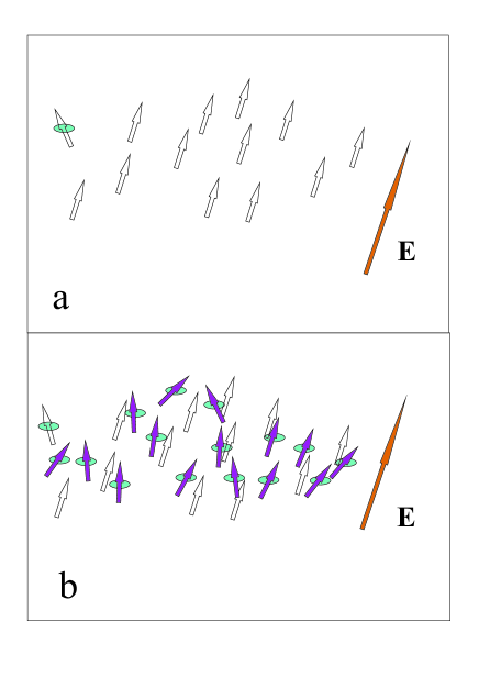
Figure 4: (Color online) The figure describes how the polarization direction perturbation propagates through the system of particles. We consider system of dipoles at $T=0$ and being in an external uniform electric field. Upper picture shows that if at the first moment there is a perturbation of the EDM, in next moment, this perturbation passes to several neighbors. At lower picture, particles in two different moments of time are described. White dipoles presents system in the first moment of time, when one dipole is perturbed only, but violet dipoles present system in the next moment.

II The model

The term describing DDI in the GP equation, for both the EDM and the magnetic moment, is interpreted via the dipole scattering length (DSL) $a_{dd}$. The GP equation does not contain information about evolution of the dipole direction. Changing of the dipole direction appears due to the interaction. If we have an external static uniform electric field, at close to zero temperatures, all dipoles will be directed parallel to the external field. At low temperatures, there is no temperature disorientation of dipoles and we have system of parallel dipoles, as it is shown on Fig. 2. In such systems, there are two type of dipoles motion. The first one is a motion, where the direction of dipoles preserves (see Fig.s 2, 3). The DDI leads to anisotropy of interaction in the BEC. At such form of motion the polarization is changed accordingly to the particle concentration $\textbf{P}(\textbf{r},t)=\textbf{d}n(\textbf{r},t)$, where d is the EDM of single particle, this motion is depicted on the Fig. 3. The second type of motion is a motion of dipoles including change of dipole direction described on the Fig.s 4, 5. Perturbation of dipole direction can be caused by both external influence and local fluctuation of direction of other dipoles produced by the DDI. In consequence of the DDI, a perturbation will propagate through the system. Particularly, this propagation might have wave nature. We need to know how polarization of system evolves in different point of space during the time for description of such motion. Therefore we need to derive equations describing the evolution of polarization field and accounting influence of interaction on this evolution.

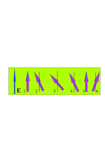
Figure 5: (Color online) The figure presents the oscillation of the EDM near of the equilibrium position which defined by the external electric field E. Indexes 1-6 present the different moments of time $t_{1}<t_{2}<...<t_{6}$. This figure describes mechanism of the polarization change due to oscillations of the EDM of each particle in the system. This mechanism might reveal along with rotation of the EDM. Incoherent motion of the EDMs which is combination of rotation and oscillation is presented on Fig. 4(b).

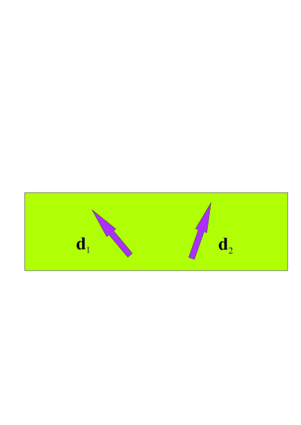
Figure 6: (Color online) The figure presents the two dipoles with the EDM turned in different directions. At propagation of perturbation through the system relative directions of dipoles is changed. This lied to change of force of interaction in concordance with potential of the DDI (2). In Appendix B we shown that the GP equation describes motion for parallel dipoles only.

In this case dipoles in different areas of space have different directions Fig. 6 and it reflects on interaction via angle dependence under integral in the GP equation (1). Still, this equation does not contain information about propagation of dipoles direction perturbation.

At studying we pay attention for the SRI and DDI. We also consider the action of external fields on particles. We consider the action of external electric field on dipoles in explicit form and the external field describing trap presented in general form by trapping potential $V_{trap}(\textbf{r}_{i},t)$.

We used quasi-static approximation for the DDI. The quasi-static approximation means that we consider interaction between dipoles at fixed moment of time as they are motionless. The DDI leads to change of state of motion, and, in particularly, to variation of dipole direction. Then, we talk about change of direction we mean both the variation during precession around of rotation axis and deviation of rotation axis direction. Described approximation is an analog of the Coulomb interaction, where interaction between moving charges approximately described by means of interaction potential of motionless charges, this approximation usually used for description of non-relativistic plasmas  Akhiezer .

Explicit form of the Hamiltonian of considering system in the quasi-static approximation is

$$\hat{H}=\sum_{i}\Biggl{(}\frac{1}{2m_{i}}\hat{\textbf{p}}_{i}^{2}-\textbf{d}_{i}\textbf{E}_{i,ext}+V_{trap}(\textbf{r}_{i},t)\Biggr{)}$$

$$+\frac{1}{2}\sum_{i,j\neq i}\Biggl{(}U_{ij}-d_{i}^{\alpha}d_{j}^{\beta}G_{ij}^{\alpha\beta}\Biggr{)}.$$ (2)

The first term in the Hamiltonian is the operator of the kinetic energy. The second term presents the interaction between the dipole moment $d_{i}^{\alpha}$ and the external electrical field. The subsequent terms present the short-range $U_{ij}$ and the dipole-dipole interactions between particles, respectively. The Green function of the dipole-dipole interaction reads as $G_{ij}^{\alpha\beta}=\nabla^{\alpha}_{i}\nabla^{\beta}_{i}(1/r_{ij})$.

For investigation of the CE dynamics in the polarized BEC we derive set of the QHD equations. This system of equations consists of the continuity equation, the Euler equation and, for the case of polarized particles, the equations of polarization evolution and equations of field (the Maxwell equations). The system of equations is derived by methods described in Ref.  Andreev PRA08 .

The first equation of the QHD equation set is the continuity equation

$$\partial_{t}n(\textbf{r},t)+\partial^{\alpha}(n(\textbf{r},t)v^{\alpha}(\textbf{r},t))=0.$$ (3)

The momentum balance equation for the polarized BEC appears as

$$mn(\textbf{r},t)(\partial_{t}+\textbf{v}\nabla)v^{\alpha}(\textbf{r},t)+\partial_{\beta}p^{\alpha\beta}(\textbf{r},t)$$

$$-\frac{\hbar^{2}}{4m}\partial^{\alpha}\triangle n(\textbf{r},t)+\frac{\hbar^{2}}{4m}\partial^{\beta}\Biggl{(}\frac{\partial^{\alpha}n(\textbf{r},t)\cdot\partial^{\beta}n(\textbf{r},t)}{n(\textbf{r},t)}\Biggr{)}$$

$$=\Upsilon n(\textbf{r},t)\partial^{\alpha}n(\textbf{r},t)+\frac{1}{2}\Upsilon_{2}\partial^{\alpha}\triangle n^{2}(\textbf{r},t)$$

$$+P^{\beta}(\textbf{r},t)\partial^{\alpha}E^{\beta}(\textbf{r},t),$$ (4)

where

$$\Upsilon=\frac{4\pi}{3}\int dr(r)^{3}\frac{\partial U(r)}{\partial r},$$ (5)

and

$$\Upsilon_{2}\equiv\frac{\pi}{30}\int dr(r)^{5}\frac{\partial U(r)}{\partial r}.$$ (6)

In equation (4) we defined a parameter $\Upsilon_{2}$ as (6). This definition differs from the one in the paper  Andreev PRA08 . Terms proportional to $\hbar^{2}$ appear as a result of using of quantum kinematics. The first two terms in the right-hand side of the equation (4) are the first terms of expansion of the quantum stress tensor. They occur because of taking into account of the SRI potential $U_{ij}$. The interaction potential $U_{ij}$ determines the macroscopic interaction constants $\Upsilon$ and $\Upsilon_{2}$. The last two terms in the equation (4) describe force fields that affect the dipole moment in a unit of volume as the effect of the external electrical field and the field produced by other dipoles, respectively. The last term is written using the self-consistent field approximation  MaksimovTMP 1999 ,  Andreev PRB 11 . $p^{\alpha\beta}(\textbf{r},t)$ is the kinetic pressure tensor, which depends on the thermal velocities of particles and does not contribute into the BEC dynamics at temperatures near zero.

The first order of the interaction radius interaction constant for dilute gases has the form

$$\Upsilon=-\frac{4\pi\hbar^{2}a}{m},$$ (7)

where $a$ is the scattering length (SL)  L.P.Pitaevskii RMP 99 ; Andreev PRA08 . The value $\Upsilon_{2}$ may be expressed approximately as

$$\Upsilon_{2}=-\frac{\theta a^{2}\Upsilon}{8},$$ (8)

where $\theta$ is a constant positive value about 1, which depends on the interatomic interaction potential. Finally, $\Upsilon_{2}$ takes the form

$$\Upsilon_{2}=-\frac{\pi\theta\hbar^{2}a^{3}}{2m}.$$ (9)

We have also equations of field

$$\nabla\textbf{E}(\textbf{r},t)=-4\pi\nabla\textbf{P}(\textbf{r},t),$$ (10)

and

$$\nabla\times\textbf{E}(\textbf{r},t)=0,$$ (11)

which are the Maxwell equation.

In the case of particles having no dipole moment, the continuity equation and the momentum balance equation form a closed set of equations. When the dipole moment is taken into account in the momentum balance equation, a new physical value emerges, it is the polarization vector field $P^{\alpha}(\textbf{r},t)$. Thus, the set of equations is not closed.

Next equation we need for studying of the CE dispersion is the polarization evolution equation

$$\partial_{t}P^{\alpha}(\textbf{r},t)+\partial^{\beta}R^{\alpha\beta}(\textbf{r},t)=0,$$ (12)

where $R^{\alpha\beta}(\textbf{r},t)$ is the current of polarization.

Equation (12) does not contain information about the effect of the interaction on the polarization evolution. An evolution equation of $R^{\alpha\beta}(\textbf{r},t)$ can be obtained by analogy with the equations derived above. Method of the equations derivation is described in Appendix A. Using the self-consistent field approximation for the dipole-dipole interaction we obtain an equation for the polarization current $R^{\alpha\beta}(\textbf{r},t)$ evolution

$$\partial_{t}R^{\alpha\beta}(\textbf{r},t)+\partial^{\gamma}\biggl{(}R^{\alpha\beta}(\textbf{r},t)v^{\gamma}(\textbf{r},t)$$

$$+R^{\alpha\gamma}(\textbf{r},t)v^{\beta}(\textbf{r},t)-P^{\alpha}(\textbf{r},t)v^{\beta}(\textbf{r},t)v^{\gamma}(\textbf{r},t)\biggr{)}$$

$$+\frac{1}{m}\partial^{\gamma}r^{\alpha\beta\gamma}(\textbf{r},t)-\frac{\hbar^{2}}{4m^{2}}\partial_{\beta}\triangle P^{\alpha}(\textbf{r},t)$$

$$+\frac{\hbar^{2}}{8m^{2}}\partial^{\gamma}\biggl{(}\frac{\partial_{\beta}P^{\alpha}(\textbf{r},t)\partial_{\gamma}n(\textbf{r},t)}{n(\textbf{r},t)}+\frac{\partial_{\gamma}P^{\alpha}(\textbf{r},t)\partial_{\beta}n(\textbf{r},t)}{n(\textbf{r},t)}\biggr{)}$$

$$=\frac{1}{m}\Upsilon\partial^{\beta}\biggl{(}n(\textbf{r},t)P^{\alpha}(\textbf{r},t)\biggr{)}$$

$$+\frac{\sigma}{m}\frac{P^{\alpha}(\textbf{r},t)P^{\gamma}(\textbf{r},t)}{n(\textbf{r},t)}\partial^{\beta}E^{\gamma}(\textbf{r},t),$$ (13)

where $r^{\alpha\beta\gamma}(\textbf{r},t)$ represents the contribution of thermal movement of polarized particles into the dynamics of $R^{\alpha\beta}(\textbf{r},t)$. As we deal with the BEC, the contribution of $r^{\alpha\beta\gamma}(\textbf{r},t)$ may be neglected. The last term in the formula (13) includes both external electrical field and the self-consistent field created by particle dipoles. This term contains numerical constant $\sigma$. Approximations used in formula (13) are described in Appendix A. The first term in the right-hand side of equation (13) describes the short-range interaction.

We can see various interactions are included in the equations (4) and (13) additively. At short distances among particles the SRI and the dipole-dipole interaction act together. At large distances dipole-dipole interaction remains only.

We can see from equation (13) that change of the polarization arises from both the dipole-dipole interaction and the short range interaction. The SRI among particle leads to displacement of particles. Consequently, as particles have the EDM, there is motion of the EDM. Therefore, there is evolution of $R^{\alpha\beta}(\textbf{r},t)$.

The terms proportional to $\hbar^{2}$ have the quantum origin. They are analogs of the Bohm quantum potential in the momentum balance equilibrium.

In the Appendix C we consider the difference between equations of electrical and magnetic polarization evolution. The QHD of spinning particles with spin-orbit interaction were developed in Ref.  Andreev arxiv MM for system of charged particles, however, obtained where force field can be used for neutral quantum gases too.

III Collective excitations in the polarized BEC

We can analyze the linear dynamics of the collective excitations in the polarized three dimensional BEC using the QHD equations (3), (4), (10), (12) and (13). Let’s assume that the system is placed in an external electrical field $\textbf{E}_{0}=E_{0}\textbf{e}_{z}$. The values of concentration $n_{0}$ and polarization $\textbf{P}_{0}=\kappa\textbf{E}_{0}$ for the system in an equilibrium state are constant and uniform and corresponding values of the velocity field $v^{\alpha}(\textbf{r},t)$ and tensor $R^{\alpha\beta}(\textbf{r},t)$ equal to zero.

We consider small perturbations of the equilibrium state as

$$\begin{array}[]{ccc}n=n_{0}+\delta n,&\textbf{v}=0+\textbf{v},&\textbf{E}=\textbf{E}_{0}+\delta\textbf{E},\end{array}$$

$$\begin{array}[]{ccc}&&P^{\alpha}=P_{0}^{\alpha}+\delta P^{\alpha},R^{\alpha\beta}=0+\delta R^{\alpha\beta}.\end{array}$$ (14)

Substituting these formulas in equations (3), (4), (12), (13) and (10) and neglecting nonlinear terms, we obtain a system of linear homogeneous equations in partial derivatives with constant coefficients. Passing to the following representation for small perturbations $\delta f$

$$\delta f=f(\omega,\textbf{k})exp(-\imath\omega t+\imath kz)$$

yields the homogeneous system of algebraic equations, where we consider wave propagation along the external elctric field. In this case the equilibrium polarization gives maximum contribution. The electric field strength is assumed to have a nonzero value. Expressing all the quantities entering the system of equations in terms of the electric field, we come to the equation

$$\Lambda\cdot\delta E_{z}=0,$$

where

$$\Lambda=\omega^{2}-\frac{\hbar^{2}k^{4}}{4m^{2}}+\frac{\Upsilon k^{2}n_{0}}{2m}+4\pi\sigma\frac{P_{0}^{2}k^{2}}{mn_{0}}$$

$$-\frac{2\pi\Upsilon k^{4}P_{0}^{2}}{m^{2}\omega^{2}-\hbar^{2}k^{4}/4+m\Upsilon k^{2}n_{0}-m\Upsilon_{2}k^{4}n_{0}}.$$

In this case, the dispersion equation is

$$\Lambda=0.$$

Solving this equation with respect to $\omega^{2}$ we obtain the following results.

The dispersion characteristic of the CE in the DBEC can be expressed in the form of

$$\omega^{2}=\frac{1}{2m}\Biggl{(}-\frac{3}{2}\Upsilon n_{0}k^{2}+\frac{\hbar^{2}k^{4}}{2m}+\Upsilon_{2}n_{0}k^{4}+4\pi\sigma\frac{P_{0}^{2}k^{2}}{n_{0}}$$

$$\pm\sqrt{\biggl{(}\frac{1}{2}\Upsilon n_{0}k^{2}-\Upsilon_{2}n_{0}k^{4}+4\pi\sigma\frac{P_{0}^{2}k^{2}}{n_{0}}\biggr{)}^{2}-8\pi\Upsilon k^{4}P_{0}^{2}}\Biggr{)}.$$ (15)

In contrast to the non-polarized BEC, where the Bogoliubov mode exists only  Bogoliubov N.1947 ; L.P.Pitaevskii RMP 99 ; Andreev PRA08 , a new wave solution appears in the polarized system due to the polarization dynamics. The Bogoliubov mode corresponds to a solution of the equation (15) with minus sign before the square root. New wave solution is a wave of polarization. In general case presented by formula (15) the frequency of polarization wave in the BEC depends on $P_{0}$ and $\Upsilon$. To investigate the BEC polarization effect on the Bogoliubov mode and the dispersion characteristic of the new solution we analyze limit cases of the formula (15). If we consider wave propagation at an angle $\theta$ to the direction of the external field we find that we should put $P_{0}\cos\theta$ instead of $P_{0}$ in equation (15).

Formula (15) demonstrates that taking into account of polarization dynamics in the BEC leads to a new solution.

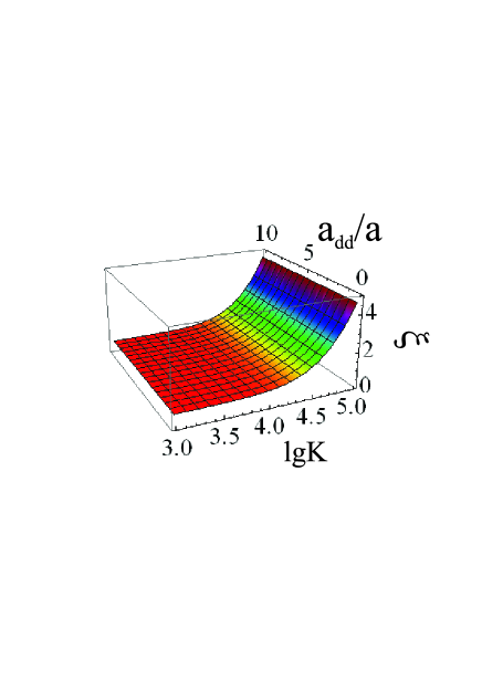
Figure 7: (Color online) The figure presents the dependence of reduced frequency $\xi$ on the wave vector $k$ and DSL $a_{dd}/|a|$ for the Bogoliubov mode. We use $\lg k$, where $k$ measured in cm^-1. Figure is obtained for the repulsive SRI $a>0$, $\Upsilon<0$, $|a|=10^{-7}$ cm, $n_{0}=10^{14}$ cm^-3, $\sigma=1$, $\theta=1$.

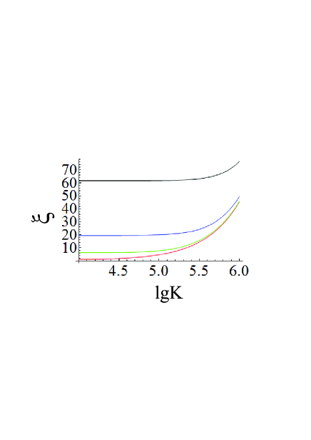
Figure 8: (Color online) The figure presents the dependence of reduced frequency $\xi$ on the wave vector $k$ for polarization wave at four different values of the DSL $a_{dd}$: $a_{dd,1}=0$ (red), $a_{dd,2}=|a|$ (green), $a_{dd,3}=10|a|$ (blue), $a_{dd,4}=100|a|$(black). We use $\lg k$, where $k$ is measured in cm^-1. Figure shows increasing of $\xi$ with increasing of $a_{dd}$. Figure is obtained for repulsive SRI $a>0$, $\Upsilon<0$, and $|a|=10^{-7}$ cm, $n_{0}=10^{14}$ cm^-3, $\sigma=1$, $\theta=1$.

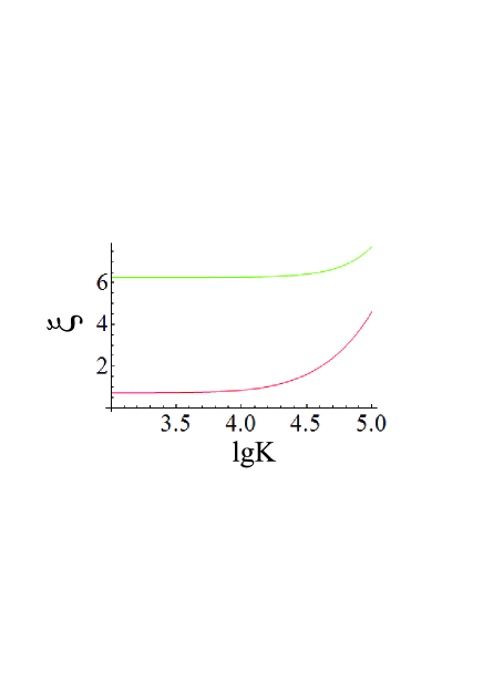
Figure 9: (Color online) The figure shows behavior of reduced frequency $\xi$ dependence on wave vector $k$ for both solutions presented by formula (16). We can see the relative behavior of two solutions. Upper curve (blue) coincides to solution with sign ”+” in front of square root (polarization mode) and lower curve (red) correspond to the one with sign ”-” (the Bogoliubov mode). The figure presents comparison of the reduced frequencies dependence for the Bogoliubov and polarization modes. We can see that $\xi(k)$ for polarization mode lie above the Bogoliubov mode. We use $\lg k$, where $k$ is measured in cm^-1. $a_{dd}=|a|$, $a>0$, $\Upsilon<0$ (repulsion), $|a|=10^{-7}$ cm, $n_{0}=10^{14}$ cm^-3, $\sigma=1$, $\theta=1$.

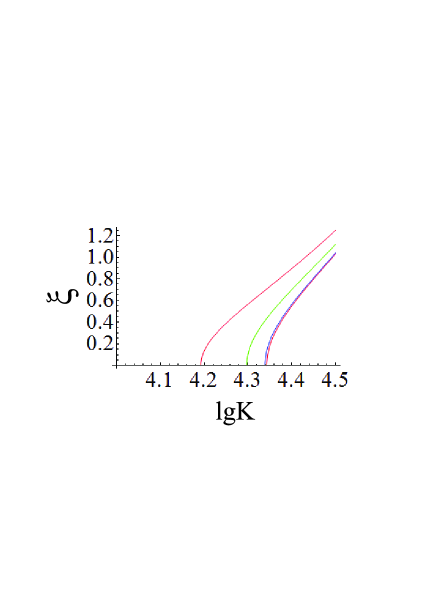
Figure 10: (Color online) The figure presents the dependence of reduced frequency $\xi$ on the wave vector $k$ for the Bogoliubov mode, $a<0$, $\Upsilon>0$ (attraction), the DSL $a_{dd}=0$ (Red, the right-hand one), $a_{dd}=0.0005|a|$ (Blue), $a_{dd}=0.005|a|$ (Green), $a_{dd}=100|a|$ (Red, the left-hand one). We use $\lg k$, where $k$ is measured in cm^-1. $|a|=10^{-7}$ cm, $n_{0}=10^{14}$ cm^-3, $\sigma=1$, $\theta=1$.

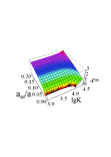
Figure 11: (Color online) The figure presents the dependence reduced frequency $\xi$ on the wave vector $k$ and the DSL $a_{dd}$ for polarization mode, $a<0$, $\Upsilon>0$ (attraction). We use $\lg k$, where $k$ is measured in cm^-1. $|a|=10^{-7}$ cm, $n_{0}=10^{14}$ cm^-3, $\sigma=1$, $\theta=1$.

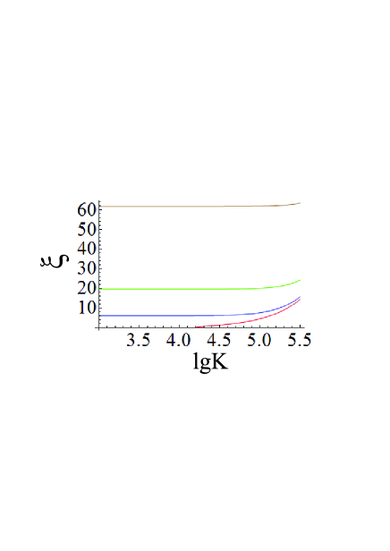
Figure 12: (Color online) The figure presents the dependence reduced frequency $\xi$ on the wave vector $k$ for the polarization mode, $a<0$, $\Upsilon>0$ (attraction), DSL $a_{dd}=0$ (Red), $a_{dd}=|a|$ (Blue), $a_{dd}=10|a|$ (Green), $a_{dd}=100|a|$ (Brown). We use $\lg k$, where $k$ is measured in cm^-1. $|a|=10^{-7}$ cm, $n_{0}=10^{14}$ cm^-3, $\sigma=1$, $\theta=1$.

Let us start with the case when contributions of different term in formula (15) are comparable. In this case we study dispersion numerically. For this purpose we represent formula (15) in the following form

$$\xi^{2}=\biggl{(}\frac{3}{4}\frac{a}{|a|}+\frac{k^{2}}{16\pi n_{0}|a|}-\frac{\theta a^{3}k^{2}}{16|a|}+\frac{6\pi\sigma a_{dd}}{|a|}$$

$$\pm\sqrt{\biggl{(}-\frac{1}{4}\frac{a}{|a|}+\frac{\theta a^{3}k^{2}}{16|a|}+\frac{6\pi\sigma a_{dd}}{|a|}\biggr{)}^{2}+\frac{6\pi a_{dd}}{a}}\biggr{)},$$ (16)

where

$$\xi^{2}\equiv\frac{\omega^{2}}{|\Upsilon|n_{0}k^{2}/m},$$

and we use the length $a_{dd}$ measures the strength of dipolar interaction, and defined by formula

$$a_{dd}=\frac{mP_{0}^{2}}{12\pi n_{0}^{2}\hbar^{2}}.$$

Above we have discussed that we do not consider the scattering process, but analogy with the results of other papers we introduced an effective parameter $a_{dd}$ describing contribution of the DDI, although $a_{dd}$ does not connect with scattering.

In the following we describe a numerical analysis of formula (16). Reduced frequency $\xi$ for two waves presented by formula (16) is exhibited on Fig.s 7 and 8. They are obtained for the repulsive SRI ($a>0$, $\Upsilon<0$) at $a=10^{-7}$cm and $n_{0}=10^{14}$cm^-3. These Fig.s show the reduced frequency $\xi(k)$ for different values of equilibrium polarization and, consequently, for different DSL $a_{dd}$.

Fig. 7 presents solution with sign ”-” in front of the square root in formula (15), this solution corresponds to the Bogoliubov mode. For all $a_{dd}/|a|$ the $\xi(k)$ does not depend on $a_{dd}/|a|$.

Fig. 8 shows strong dependence of the reduced frequency of the polarization mode (”+” in front of the square root in formula (15)) on equilibrium polarization. On Fig.8 as on other Fig.s this dependence is presented via dependence on the DSL divided on module of the SL of SRI $a_{dd}/|a|$.

The form of $\xi(k)$ for two solutions has similar form. We present both solutions on Fig. 9 at fixed $a_{dd}/|a|=1$ to compare. From Fig. 9 we see that the reduced frequency of polarization mode is larger than one for Bogoliubov mode.

From the Fig.8 we obtain that polarization lead to growing of the reduced frequency $\xi$ of the polarization mode. The reduced frequency $\xi$ increases in 6 times at small wave vectors of order $10^{4}$cm^-1 and for the $a_{dd}=|a|$. For the $a_{dd}=100|a|$ increases in 60 times. With increasing of wave vector the influence of polarization becames smaller. For example at $k=10^{6}$cm^-1 and $a_{dd}=100|a|$ the reduced frequency $\xi$ increase just in 1.6 times.

For the case of an attractive SRI in the absence of the polarization there is instability of the Bogoliubov mode at small wave vectors. At the presence of small polarization the Bogoliubov mode remains unstable, but the area of stability become some wider as it is shown on Fig. 10. There is fast widening of the region of stability at increasing of $a_{dd}/|a|$ Fig. 11. Widening starts at approximately $a_{dd}=0.02|a|$.

For the case of the attractive SRI in the absence of polarization there is instability of polarization mode at small wave vectors (see Fig. 12). At $a_{dd}=0$ we see instability of waves at wave vector $k$ below $1.6\cdot 10^{4}$cm^-1. The EDM leads to increasing of $\xi$ and fast growing of the region of stability. The wave is stable up to $k=10^{3}$cm^-1 at $a_{dd}/|a|=1$. Further increasing of $a_{dd}/|a|$ leads to increasing of $\xi$ up to 64. $\xi$ become equal to 64 at $a_{dd}/|a|\simeq 100$ and does not change at further increasing of $a_{dd}/|a|$.

Comparing Fig.s 10 and 12 we can see that reduced frequency $\xi$ of polarization mode much larger than the Bogoliubov mode, as it was for the repulsive SRI.

With increasing of strength of the SRI the role of $\Upsilon_{2}$ become more important. It’s influence reveals at $|a|=10^{-5}$cm for the attractive SRI. In this case, there is instability region at relatively large wave vectors. For described case the reduced frequency $\xi(k)$ is presented on Fig.s 13 and 14 at various $a_{dd}/|a|$. The region of instability is shown there. This instability appears because the expression under the square root in formula (15) became negative as it shown on Fig. 15.

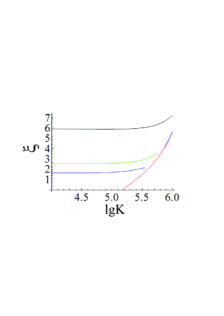
Figure 13: (Color online) The figure presents the dependence of the reduced frequency $\xi$ on the wave vector $k$ for the polarization mode. On this Fig. the region of instabilities is also shown. It is a region, where we see a gap in curves. Figure obtained for the attractive SRI ($a<0$, $\Upsilon>0$), $a_{dd}=0$ (Red), $a_{dd}=0.1|a|$ (Blue), $a_{dd}=0.2|a|$ (Green), $a_{dd}=|a|$ (Black). We use $\lg k$, where $k$ is measured in cm^-1. $|a|$= 10^-5 cm, $n_{0}=10^{14}$ cm^-3, $\sigma=1$, $\theta=1$.

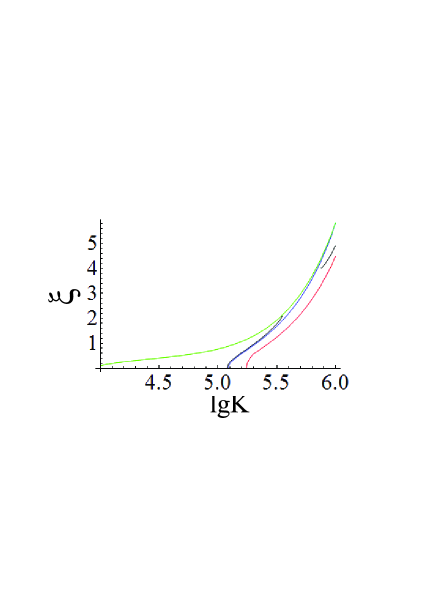
Figure 14: (Color online) The figure presents the dependence of the reduced frequency $\xi$ on the wave vector $k$ for the Bogoliubov mode, $a<0$, $\Upsilon>0$ (attraction), the DSL $a_{dd}=0$ (Red), $a_{dd}=0.1|a|$ (Black), $a_{dd}=0.2|a|$ (Blue), $a_{dd}=2|a|$ (Green). We use $\lg k$, where $k$ is measured in cm^-1. $|a|$= 10^-5 cm, $n_{0}=10^{14}$ cm^-3, $\sigma=1$, $\theta=1$.

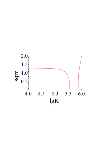
Figure 15: (Color online) The figure presents the behavior of the square root in formula (32) (we conditionally designated this quantity as ”sqrr”) at different values of the wave vector $k$ corresponding to the Fig. 10 at $a_{dd}=0.1|a|$, (square does not depend on concentration). $|a|$= 10^-5 cm, $\sigma=1$, $\theta=1$. We use $\lg k$, where $k$ is measured in cm^-1.

Below, we analytically consider limit cases of general dispersion solution (15).

We now proceed to derive a dispersion dependence when the effect of polarization is small in comparison with the contribution of the short-range effects, i.e. we consider a limit when the terms proportional to $\Upsilon$ and $\Upsilon_{2}$ are comparably large. Consequently, formula (15) takes the form

$$\omega^{2}_{B}=\frac{\hbar^{2}k^{4}}{4m^{2}}-\frac{\Upsilon n_{0}k^{2}}{m}+\frac{\Upsilon_{2}n_{0}k^{4}}{m}$$

$$-\frac{4\pi P_{0}^{2}k^{2}}{mn_{0}}\frac{\Upsilon(\sigma-1)-2\sigma\Upsilon_{2}k^{2}}{\Upsilon-2\Upsilon_{2}k^{2}},$$ (17)

and

$$\omega^{2}_{P}=\frac{\hbar^{2}k^{4}}{4m^{2}}-\frac{1}{2}\frac{\Upsilon n_{0}k^{2}}{m}$$

$$+\frac{4\pi P_{0}^{2}k^{2}}{mn_{0}}\frac{\Upsilon(\sigma-1)-2\sigma\Upsilon_{2}k^{2}}{\Upsilon-2\Upsilon_{2}k^{2}},$$ (18)

where we use indexes ”B” for the Bogoliubov mode and ”P” for new polarization mode. At derivation of formulas (17) and (18) we expanded a sub-radical expression in (15) and took only first two terms of the expansion to estimate the influence of polarization on the wave dispersion.

As it follows from equations (12) and (13), changes of polarization can occur due to the dipole-dipole interactions, the SRI and the quantum Bohm potential (terms proportional to $\hbar^{2}$). This is the reason for existence of other ways of polarization changing when the contribution of equilibrium polarization $P_{0}$ is negligible. In described case, changes in the polarization do not affect the concentration evolution in linear approximation.

Formula (15) is valid even in absence of the external electrical field when equilibrium polarization equals to zero $P_{0}=0$. In this case, equations (15) appears as

$$\omega^{2}_{B}=\frac{1}{m}\Biggl{(}\frac{\hbar^{2}k^{4}}{4m}-\Upsilon n_{0}k^{2}+\Upsilon_{2}n_{0}k^{4}\Biggr{)},$$ (19)

and

$$\omega^{2}_{P}=\frac{1}{2m}\Biggl{(}\frac{\hbar^{2}k^{4}}{2m}-\Upsilon n_{0}k^{2}\Biggr{)}.$$ (20)

The waves of polarization can exist at the absence of external electric field $E_{0}=0$. In this case the equilibrium state is not polarized and dipole direction of particles is distributed accidentally.

If the contribution of equilibrium polarization in the BEC dispersion (15) is comparable to the contribution of the SRI in the third order by the interaction radius $\Upsilon_{2}$ (15) transforms into

$$\omega^{2}_{B}=\frac{\hbar^{2}k^{4}}{4m^{2}}-\frac{\Upsilon n_{0}k^{2}}{m}+\frac{\Upsilon_{2}n_{0}k^{4}}{m}+4\pi\frac{P_{0}^{2}k^{2}}{mn_{0}},$$ (21)

and

$$\omega^{2}_{P}=\frac{\hbar^{2}k^{4}}{4m^{2}}-\frac{1}{2}\frac{\Upsilon n_{0}k^{2}}{m}+4\pi\frac{P_{0}^{2}k^{2}}{mn_{0}}(\sigma-1).$$ (22)

Using Feshbach resonance  Chin RMP 10 ; Bloch RMP 08 we can tune the SRI potential that $\Upsilon=0$ while $\Upsilon_{2}\neq 0$. In this situation formula (15) turns into

$$\omega^{2}_{B}=\frac{\hbar^{2}k^{4}}{4m^{2}}+\frac{\Upsilon_{2}n_{0}k^{4}}{m},$$ (23)

and

$$\omega^{2}_{P}=\frac{\hbar^{2}k^{4}}{4m^{2}}+4\pi\sigma\frac{P_{0}^{2}k^{2}}{mn_{0}}.$$ (24)

In this paper we primarily focus on the influence of the BEC polarization on its dispersion characteristics. So, let us consider the case when the contribution into the dispersion of the SRI at the first order of the interaction radius, i.e. terms proportional to $\Upsilon$, is comparable to the contribution of polarization, and their total effect is much larger than the contribution of terms proportional to $\Upsilon_{2}$. We find that formula (15) turns into

$$\omega^{2}_{B}=\frac{\hbar^{2}k^{4}}{4m^{2}}-\frac{\Upsilon n_{0}k^{2}}{m}\biggl{(}\frac{(\sigma-1)}{\sigma}\biggr{)},$$ (25)

and

$$\omega^{2}_{P}=\frac{\hbar^{2}k^{4}}{4m^{2}}+4\pi\sigma\frac{P_{0}^{2}k^{2}}{mn_{0}}$$

$$-\frac{1}{2}\frac{\Upsilon n_{0}k^{2}}{m}\biggl{(}\frac{(\sigma+4)}{2\sigma}\biggr{)}.$$ (26)

III.1 polarization evolution at constant concentration

The DBEC is the rare gas and we can not use condition incompressibility, but we consider the case there concentration of particles is not change in time. We are interested in dynamics of wave of polarization only. For this aim we need to use equations (12) and (13) at additional condition $n(\textbf{r},t)=n_{0}=const$. This is means the polarization changes due to evolution of dipoles direction. Equation of polarization evolution (12) has no change in this approximation. Nonlinear terms in equation (13) disappear and the term describing the SRI simplifies, so we have

$$\partial_{t}R^{\alpha\beta}(\textbf{r},t)+\partial^{\gamma}\biggl{(}R^{\alpha\beta}(\textbf{r},t)v^{\gamma}(\textbf{r},t)$$

$$+R^{\alpha\gamma}(\textbf{r},t)v^{\beta}(\textbf{r},t)-P^{\alpha}(\textbf{r},t)v^{\beta}(\textbf{r},t)v^{\gamma}(\textbf{r},t)\biggr{)}$$

$$-\frac{\hbar^{2}}{4m^{2}}\partial_{\beta}\triangle P^{\alpha}(\textbf{r},t)=\frac{n_{0}}{m}\Upsilon\partial^{\beta}\biggl{(}P^{\alpha}(\textbf{r},t)\biggr{)}$$

$$+\frac{\sigma}{mn_{0}}P^{\alpha}(\textbf{r},t)P^{\gamma}(\textbf{r},t)\partial^{\beta}E^{\gamma}(\textbf{r},t).$$ (27)

in the set with equations of field (10) and (11).

Only one wave solution exists in this approximation, it is the wave of polarization. Its dispersion is

$$\omega^{2}=\frac{\hbar^{2}k^{4}}{4m^{2}}+\biggl{(}\frac{4\pi\sigma P_{0}^{2}}{mn_{0}}-\frac{n_{0}\Upsilon}{m}\biggr{)}k^{2}.$$ (28)

Formula (28) reduces to

$$\omega^{2}=\frac{4\pi\sigma P_{0}^{2}}{mn_{0}}k^{2}$$

than polarization dominates. For the particles with the EDM equal to 1 Debye at concentration 10¹² cm^-3 and wave vector $k\simeq 10^{7}$ cm^-1 the frequency $\omega$ reach value of order $10^{6}-10^{7}$ s^-1.

Dispersion of the 1D and 2D wave of polarization is described in Ref.  Andreev PRB 11 .

IV Generation of waves in polarized BEC

In this section we consider the process of wave generation in the BEC by means of the beam of neutral polarized particles. The interaction between the beam and the BEC has the dipole-dipole origin.

To get the dispersion solution we use the system of the QHD equations for each sort of particles (3), (4), (12), (13) and the equations of field (10) and (11). The equilibrium state of system is characterized by following values of the BEC parameters:

$$\begin{array}[]{ccc}n_{B}=n_{B0}+\delta n_{B},&v^{\alpha}_{B}=0+v^{\alpha}_{B},&\end{array}$$

$$\begin{array}[]{ccc}&P^{\alpha}_{B}=P_{B0}^{\alpha}+\delta P^{\alpha}_{B},&R^{\alpha\beta}_{B}=0+\delta R^{\alpha\beta}_{B},\end{array}$$ (29)

and values of the beam parameters:

$$\begin{array}[]{ccc}n_{b}=n_{0b}+\delta n_{b},&v^{\alpha}_{b}=U\delta^{z\alpha}+\delta v^{\alpha}_{b},&\end{array}$$

$$\begin{array}[]{ccc}&P_{b}^{\alpha}=P_{0b}^{\alpha}+\delta P^{\alpha}_{b},&R^{\alpha\beta}_{b}=R^{\alpha\beta}_{0b}+\delta R^{\alpha\beta}_{b}.\end{array}$$ (30)

The polarization $P_{0}^{\alpha}$ is proportional to the external electric field $E_{0}^{\alpha}$. We consider the case then $\textbf{E}_{0}=[E_{0}sin\varphi,0,E_{0}cos\varphi]$. In this case the tensor $R^{\alpha\beta}_{0b}$ has only two nonzero elements: $R^{zx}_{0b}=R_{0b}sin\varphi$ and $R^{zz}_{0b}=R_{0b}cos\varphi$. For the process, under consideration the dispersion relation is:

$$1+4\pi k^{2}\Biggl{(}\frac{P_{0}^{2}}{\omega^{2}-\frac{\hbar^{2}k^{4}}{4m^{2}}+\frac{\Upsilon n_{0}k^{2}}{2m}}\times$$

$$\times\biggl{(}\frac{\Upsilon k^{2}/(2m^{2})}{\omega^{2}-\frac{\hbar^{2}k^{4}}{4m^{2}}+\frac{\Upsilon n_{0}k^{2}}{m}-\frac{\Upsilon_{2}n_{0}k^{4}}{m}}-\frac{\sigma}{mn_{0}}\biggr{)}$$

$$+\frac{1}{(\omega-k_{z}U)^{2}-\frac{\hbar^{2}k^{4}}{4m^{2}_{b}}}\times$$

$$\times\biggl{(}\frac{2(\omega-k_{z}U)P_{0b}k_{z}(P_{0b}U-R_{0b})}{m_{b}n_{0b}\biggl{(}(\omega-k_{z}U)^{2}-\frac{\hbar^{2}k^{4}}{4m^{2}_{b}}\biggr{)}}-\frac{\sigma_{b}P_{0b}^{2}}{m_{b}n_{0b}}\biggr{)}\Biggr{)}=0.$$ (31)

Using relation $P_{0b}U-R_{0b}=0$, we can simplify the equation (31) and obtain

$$1+\frac{\omega_{D}^{2}}{\omega^{2}-\omega_{1}^{2}}\Biggl{(}\frac{\Upsilon n_{0}k^{2}/(2m)}{\omega^{2}-\omega_{2}^{2}}-\sigma\Biggr{)}$$

$$-\frac{\sigma_{b}\omega_{Db}^{2}}{(\omega-k_{z}U)^{2}-\frac{\hbar^{2}k^{4}}{4m^{2}_{b}}}=0.$$ (32)

In this formula the following designations are used

$$\omega_{1}^{2}=\frac{\hbar^{2}k^{4}}{4m^{2}}-\frac{\Upsilon n_{0}k^{2}}{2m},$$ (33)

$$\omega_{2}^{2}=\frac{\hbar^{2}k^{4}}{4m^{2}}-\frac{\Upsilon n_{0}k^{2}}{m}+\frac{\Upsilon_{2}n_{0}k^{4}}{m}$$ (34)

and

$$\omega_{Di}^{2}=\frac{4\pi P_{0i}^{2}k^{2}}{m_{i}n_{0i}},$$ (35)

where $i$ is the index of sorts of particles, the BEC ($i=B$) or the beam ($i=b$).

The equation (32) has two beam related solutions, in the absence of BEC medium:

$$\omega=k_{z}U\pm\sqrt{\frac{\hbar^{2}k^{4}}{4m^{2}_{b}}+\sigma_{b}\omega_{Db}^{2}}.$$ (36)

We will consider the possibilities of instability for the case of low-density beam $\omega_{Db}\sim n_{0b}\rightarrow 0$. In this case we can neglect the last term under the square root in (36). The resonance interaction of beam with the BEC realizing at

$$k_{z}U\pm\frac{\hbar k^{2}}{2m_{b}}=\omega(k),$$ (37)

and could lead to instabilities. The quantity $\omega(k)$ is the dispersion of BEC modes (15). The frequency in this case can be presented in the form

$$\omega=k_{z}U\pm\frac{\hbar k^{2}}{2m_{b}}+\delta\omega.$$ (38)

Let us to consider two limit cases.

IV.1 small frequency shift limit

Under condition

$$\delta\omega\ll\hbar k^{2}/m$$ (39)

the frequency shift emerges as

$$\delta\omega^{2}=\pm\frac{2\sigma_{b}m_{b}m^{2}\omega_{Db}^{2}(\omega^{2}-\omega_{1}^{2})^{2}(\omega^{2}-\omega_{2}^{2})^{2}}{\omega\omega_{D}^{2}\hbar\Upsilon^{2}n_{0}^{2}k^{6}W},$$ (40)

where

$$W=2\omega^{2}-\omega_{1}^{2}-\omega_{2}^{2}-\frac{2m\sigma}{\Upsilon n_{0}k^{2}}(\omega^{2}-\omega_{2}^{2})^{2}.$$ (41)

and the frequency $\omega$ determined with formula (15). The instabilities take place when $\delta\omega^{2}<0$. The sign of $\delta\omega^{2}$ depends on the sign of $W$.

For the case resonance interaction of beam with the waves in BEC there are instabilities, for the first beam mode in (36) at $W<0$ and for the second beam mode in formula (36) at $W>0$. For the polarization mode $W$ is positive. It means that interaction of polarization mode with the second beam related mode results in the instability. For the Bogoliubov mode the sign of $W$ depends on $\sigma$.

We can consider the following cases:

(i) the contribution of equilibrium polarization to $\omega(k)$ is dominant; then $W>0$;

(ii) main contribution in $\omega(k)$ gives term proportional to $\Upsilon$, and, equilibrium polarization and SRI in the TOIR approximation are comparable to each other. In this case, there is a value of $\sigma$, designated as $\sigma_{0}$, which is

$$\sigma_{0}=1+\frac{\Upsilon_{2}n_{0}k^{4}/m}{\Upsilon n_{0}k^{2}/(2m)+2\Upsilon_{2}n_{0}k^{4}/m-4\omega_{D}^{2}}.$$

The sign of $W$ varies at $\sigma=\sigma_{0}$. The dependence of sign of $W$ on $\sigma$ is presented in the Table 1.

Table 1: In this table the sign of the $W$ are presented for the Bogoliubov mode when the SRI is prevailed over dipole-dipole interaction.

	$\frac{\Upsilon>0}{\textmd{attraction}}$	$\frac{\Upsilon<0}{\textmd{repulsion}}$
$\sigma>\sigma_{0}$	+	-
$\sigma<\sigma_{0}$	-	+

IV.2 large frequency shift limit

In opposite limit

$$\delta\omega\gg\hbar k^{2}/m$$ (42)

we have

$$\delta\omega=\xi\sqrt[3]{\frac{\sigma_{b}m^{2}\omega_{Db}^{2}(\omega^{2}-\omega_{1}^{2})^{2}(\omega^{2}-\omega_{2}^{2})^{2}}{\omega\omega_{D}^{2}\Upsilon^{2}n_{0}^{2}k^{4}\mid W\mid}},$$ (43)

where $\xi$ equal to $\xi_{1}=\sqrt[3]{1}$ for $W>0$ or $\xi_{-1}=\sqrt[3]{-1}$ for $W<0$. Explicit form of quantities $\xi_{1}$ and $\xi_{-1}$ are

$$\xi_{-1}=[-1,\frac{-1+\imath\sqrt{3}}{2},\frac{-1-\imath\sqrt{3}}{2}],$$

and

$$\xi_{1}=[1,\frac{1+\imath\sqrt{3}}{2},\frac{1-\imath\sqrt{3}}{2}].$$

The consideration concerning the sign of $W$, reflected in the table 1, are valid also for the limit condition (42).

From the formulas (40) and (43) we can see that neutral particles beam leads to instabilities for both the Bogoliubov and polarization waves.

V Conclusion

We developed the self-consistent method for description of the DBEC dynamics. This method accounts effect of polarization on changes of the particle concentration and velocity field, which are determined in general by the continuity equation and Euler equation. We derived the evolution equations of the polarization and the polarization current. The derived equations contain information about the influence of the interactions on the polarization evolution. We studied the effect of polarization on the BEC dynamics and influence of the SRI on the polarization evolution. An expression of the SRI contribution in the equation of polarization current evolution via concentration, polarization and the SRI potential $\Upsilon=\Upsilon(U_{ij})$ was derived. With the assumption that the state of polarized Bose particles in the form of BEC can be described with some single-particle wave function. Changes in polarization due to SRI are shown to be determined at the first order of the interaction radius by the same interaction constant that occurs in Euler’s equation and Gross-Pitaevskii equation.

The derivation of the GP equation for polarized particles from the QHD equations was obtained. The conditions of validity of the GP equation was presented. Comparison of evolution equation of the electrically polarized BEC and the magnetized BEC was discussed and differences were described.

Physical meaning of the self-consistent approximation was described. Suitability of the self-consistent approximation for electrically polarized BEC was shown. Distinctions of developed self-consistent approximation for dipole-dipole interaction from the scattering process are discussed.

Correct form of the dipole-dipole interaction Hamiltonian is discussed. The arguments for choosing of correct form of Hamiltonian for electric and magnetic dipoles are presented.

The dispersion of the CE in the polarized BEC was analyzed. We shown that polarization evolution in the BEC causes a novel type of waves. The effect of polarization on the dispersion of the Bogoliubov mode and the dispersion of a new wave mode were studied.

We shown the possibility of wave generation in the polarized BEC by means of the monoenergetic beam of neutral polarized particles.

VI Appendix A

VI.1 Correct form of Hamiltonian for dipole-dipole interaction

At derivation of the QHD equations we need to write explicit form of the Hamiltonian of dipole-dipole interaction. In some works the dynamics of the magnetic dipole moment and of the EDM  Lahaye RPP 09 ; Yi PRA 02 are analyzed in similar ways. Usual expression of the Hamiltonian for the dipole-dipole interaction for the electric and the magnetic dipoles equals

$$H_{dd}=\frac{\delta^{\alpha\beta}-3r^{\alpha}r^{\beta}/r^{2}}{r^{3}}d_{1}^{\alpha}d_{2}^{\beta}.$$ (44)

Generally speaking the Hamiltonian for the spin-spin and the electric dipole-dipole interaction are different, and they also differ from (44). All Hamiltonians contain a term proportional to the Dirac delta function. These terms have different numerical coefficient for two kind of BECs. In this paper for interaction of electric dipoles we used following Hamiltonian

$$H_{dd}=-\partial^{\alpha}\partial^{\beta}\frac{1}{r}\cdot d_{1}^{\alpha}d_{2}^{\beta},$$

which follows from potential of the electric field caused by electric dipole Landau 2 . There is well-known identity

$$-\partial^{\alpha}\partial^{\beta}\frac{1}{r}=\frac{\delta^{\alpha\beta}-3r^{\alpha}r^{\beta}/r^{2}}{r^{3}}+\frac{4\pi}{3}\delta^{\alpha\beta}\delta(\textbf{r}),$$ (45)

so we can see the difference between usually using Hamiltonian and one’s used in this paper. The corrections of our selection followed from the fact that the equations obtained in the paper coincide to the Maxwell equations. Derivation of the QHD equations in the self-consistent approximation leads to field equation (10) and (11), we rewrite them here

$$\nabla\textbf{E}(\textbf{r},t)=-4\pi\nabla\textbf{P}(\textbf{r},t),$$ (46)

and

$$\nabla\times\textbf{E}(\textbf{r},t)=0,$$ (47)

but if we used Hamiltonian (44) we would obtain

$$\nabla\textbf{E}(\textbf{r},t)=\frac{8\pi}{3}\nabla\textbf{P}(\textbf{r},t),$$ (48)

instead of (46). Using formula (44) leads to non-fulfilment of equation (47).

It has been shown by Breit  spin-spin interaction that the Hamiltonian for the spin-spin interaction contains a term proportional to the Dirac $\delta$-function $\delta(r_{1}-r_{2})d_{1}^{\alpha}d_{2}^{\beta}$ along with (44). The coefficient at the $\delta$ function was refined later  MaksimovTMP 2001 , so it was shown that the Hamiltonian is in according with the Maxwell equations (46), (47). The conclusive expression for the spin-spin interaction Hamiltonian appears as

$$H_{\mu\mu}=-\Biggl{(}4\pi\delta^{\alpha\beta}\delta(\textbf{r}_{12})+\nabla^{\alpha}_{1}\nabla^{\beta}_{1}(1/r_{12})\Biggr{)}\mu^{\alpha}_{1}\mu^{\beta}_{2},$$ (49)

or

$$H_{\mu\mu}=\Biggl{(}\frac{\delta^{\alpha\beta}-3r^{\alpha}r^{\beta}/r^{2}}{r^{3}}-\frac{8\pi}{3}\delta^{\alpha\beta}\delta(\textbf{r})\Biggr{)}\mu^{\alpha}_{1}\mu^{\beta}_{2}.$$ (50)

Thus, the differences in the dipole-dipole interactions of the electric dipoles, and the magnetic dipoles, have to be taken into account at development of theoretical field apparatus.

VI.2 Method of equations derivation

The Schrödinger equation defines wave function in the 3N-dimensional configuration space while physical processes in systems that involve large number of particles occur in the three-dimensional physical space  Goldstein . This is why a problem evolves obtaining of the quantum-mechanical description of a system of particles in terms of material fields, e.g. the particle concentration, the momentum density, the energy density and other fields of various tensor dimension that are defined in the three-dimension space.

The first step in the many-particle QHD equation derivation is the definition of particles concentration. We define the quantum particles concentration as the quantum average of the classic microscopic concentration in the coordinate representation on many-particle wave function $\psi(R,t)$. Thus, the particles concentration explicit form to be

$$n(\textbf{r},t)=\int dR\sum_{i}\delta(\textbf{r}-\textbf{r}_{i})\psi^{*}(R,t)\psi(R,t),$$

where $dR=\prod_{i=1}^{N}d\textbf{r}_{i}$. Differentiating this function over time and using the Schrodinger equation with the Hamiltonian (2), we derive the continuity equation (3). In the continuity equation the new quantity appears, it is the particle current or momentum density. We differentiate this quantity over time and use the Schrodinger equation with the Hamiltonian (2). In the results we obtain the momentum balance equation. In this way we can find an evolution equation for any additive physical quantity, but we mast know its definition. The definition of new physical quantities appears at derivation of the QHD equation. Several quantities appears at derivation of the momentum balance equation (4), one of them is the polarization presented below (51). Knowledge of the polarization definition gives possibility to derive the equation of polarization evolution (13) and so on.

In equations (4), (10) polarization occurs in the form of

$$P^{\alpha}(\textbf{r},t)=\int dR\sum_{i}\delta(\textbf{r}-\textbf{r}_{i})\psi^{*}(R,t)\hat{d}_{i}^{\alpha}\psi(R,t),$$ (51)

where $\textbf{r}_{i}$ is the coordinate of i-th particle, $dR=\prod_{p=1}^{N}d\textbf{r}_{p}$.

In the right-hand side of equation (13), where is the force-like field $F^{\alpha\beta}(\textbf{r},t)$ which gives rise to evolution of the polarization current $R^{\alpha\beta}(\textbf{r},t)$. In general case, for $F^{\alpha\beta}(\textbf{r},t)$, we can write:

$$F^{\alpha\beta}(\textbf{r},t)=-\frac{1}{m}\partial_{\gamma}\Sigma^{\alpha\beta\gamma}(\textbf{r},t)+\frac{1}{m}D^{\alpha\gamma}(\textbf{r},t)\partial^{\beta}E^{\gamma}(\textbf{r},t).$$ (52)

The tensor

$$D^{\alpha\beta}(\textbf{r},t)=\int dR\sum_{i}\delta(\textbf{r}-\textbf{r}_{i})d_{i}^{\alpha}d_{i}^{\beta}\psi^{*}(R,t)\psi(R,t),$$ (53)

occurs in the term that presents the dipole-dipole interaction and an interaction of the dipole with an external electrical field. This value can be approximately presented as

$$D^{\alpha\beta}(\textbf{r},t)=\sigma\frac{P^{\alpha}(\textbf{r},t)P^{\beta}(\textbf{r},t)}{n(\textbf{r},t)},$$ (54)

that based on the reasons of dimensions.

The SRI causes the tensor $\Sigma^{\alpha\beta\gamma}(\textbf{r},t)$ to occur in the equation (13). Taken at the first order by the interaction radius it has the form

$$\Sigma^{\alpha\beta\gamma}(\textbf{r},t)=-\frac{1}{2}\int dR\sum_{i,j\neq i}\delta(\textbf{r}-\textbf{R}_{ij})$$

$$\times\frac{r_{ij}^{\beta}r_{ij}^{\gamma}}{r_{ij}}\frac{\partial U_{ij}}{\partial r_{ij}}\psi^{*}(R,t)\hat{d}_{i}^{\alpha}\psi(R,t).$$ (55)

Tensor $\Sigma^{\alpha\beta\gamma}(\textbf{r},t)$ describes the influence of the SRI on evolution of polarization. Formula (55) describes the SRI.

If we apply the procedure described in Ref.  Andreev PRA08 to calculate the quantum stress tensor, and neglect the contribution of the thermal effects, when $\Sigma^{\alpha\beta\gamma}(\textbf{r},t)$, for the BEC, takes the following form

$$\Sigma^{\alpha\beta\gamma}_{BEC}(\textbf{r},t)=-\frac{1}{2}\Upsilon\delta^{\beta\gamma}n(\textbf{r},t)P^{\alpha}(\textbf{r},t).$$ (56)

Formula (56) is obtained for particles located in state with the lowest energy, which can be described by one particle wave function. However, this state may be the product of strong interaction. Tensor $\Sigma^{\alpha\beta\gamma}(\textbf{r},t)$, therefore, like the quantum stress tensor $\sigma^{\alpha\beta}(\textbf{r},t)$ in the momentum balance equation (4), depends on $\Upsilon$ at the first order by the interaction radius  Andreev PRA08 .

VII Appendix B: Derivation of the non-linear Schrödinger equation

A derivation of GP equation was performed for non-polarized particles from the QHD equations  Andreev PRA08 , here we present one for particles having electric dipole moment. The NLSE comes from the continuity equation (3) and the Cauchy integral of the momentum balance equation (4). The Cauchy integral exists if the velocity field can be expressed as

$$v^{\alpha}(\textbf{r},t)=\frac{1}{m}\partial^{\alpha}\theta(\textbf{r},t)$$ (57)

where $\theta(\textbf{r},t)$ is the velocity field potential.

Starting from the QHD equations we can derive an equation for evolution of a model function defined in terms of hydrodynamic variables. Thus, the macroscopic single-particle wave function may be defined as

$$\Phi(\textbf{r},t)=\sqrt{n(\textbf{r},t)}\exp\biggl{(}\frac{\imath}{\hbar}m\theta(\textbf{r},t)\biggr{)}.$$ (58)

If we differentiate this function with respect to time and apply the QHD equations when we obtain

$$\imath\hbar\partial_{t}\Phi(\textbf{r},t)=\Biggl{(}-\frac{\hbar^{2}}{2m}\nabla^{2}+\Gamma(\textbf{r},t)+g\mid\Phi(\textbf{r},t)\mid^{2}$$

$$-\int_{\textbf{r}_{0}}^{\textbf{r}}d\textbf{r}^{\prime}\frac{1}{n(\textbf{r}^{\prime},t)}P^{\beta}(\textbf{r}^{\prime},t)\times$$

$$\times\nabla^{\prime}\int d\textbf{r}^{\prime\prime}G^{\beta\gamma}(\textbf{r}^{\prime},\textbf{r}^{\prime\prime})P^{\gamma}(\textbf{r}^{\prime\prime},t)\Biggr{)}\Phi(\textbf{r},t),$$ (59)

here we use designation $\Gamma(\textbf{r},t)$ described by formula

$$\Gamma(\textbf{r},t)=\int_{\textbf{r}_{0}}^{\textbf{r}}d\textbf{r}^{\prime}\frac{\nabla p(\textbf{r}^{\prime},t)}{n(\textbf{r}^{\prime},t)}.$$ (60)

Quantity $\Gamma(\textbf{r},t)$ can be considered as chemical potential $\mu(\textbf{r},t)$ and we use this below. The equation (59) has the form of a NLSE. A NLSE with the DDI was obtained in Ref.  Andreev PRB 11 , where the sign ”-” was lost in front of integral in formulas (A6) and (A8).

The NLSE (59) describes collective properties of the many particles system. This follows from the derivation of the NLSE and from the definition of the many-particle wave function $\Phi(\textbf{r},t)$ (58). Function $\Gamma(\textbf{r},t)$ (60) is the contribution of the kinetic pressure and does not contain any interaction.

If we introduce a function $d^{\alpha}(\textbf{r},t)$ as $d^{\alpha}(\textbf{r},t)=P^{\alpha}(\textbf{r},t)/n(\textbf{r},t)$ and if also we suppose that $d^{\alpha}(\textbf{r},t)$ is a constant $d^{\alpha}$, when we obtain

$$\imath\hbar\partial_{t}\Phi(\textbf{r},t)=\Biggl{(}-\frac{\hbar^{2}}{2m}\nabla^{2}+\mu(\textbf{r},t)+g\mid\Phi(\textbf{r},t)\mid^{2}$$

$$-d^{\beta}d^{\gamma}\int d\textbf{r}^{\prime}G^{\beta\gamma}(\textbf{r},\textbf{r}^{\prime})|\Phi(\textbf{r}^{\prime},t)|^{2}\Biggr{)}\Phi(\textbf{r},t)$$ (61)

from equation (59), we have used that $n(\textbf{r},t)=|\Phi(\textbf{r},t)|^{2}$.

At the temperature $T$ equal to zero in external electric field $\textbf{E}_{0}$ all dipoles directed parallel to external field. If $\textbf{E}_{0}=E_{0}\textbf{e}_{z}$ we have $\textbf{d}=d_{0}\textbf{e}_{z}$. In this case in equation (61) only one component of Green function $G^{\beta\gamma}$ of the DDI is nonzero, it is $G^{zz}$, which has following form $G^{zz}=(1-3z^{2}/r^{2})/r^{3}+4\pi/3\cdot\delta(\textbf{r})$. we obtain the GP equation (1) presented in introduction at the absence of $\delta$ function from (61) and using relation $z^{2}/r^{2}=\cos^{2}\theta$.

The GP equation was obtained for the case of system of parallel dipoles. We suppose it can be approximately used for analyze of dipoles whose direction slowly changed in space.

VIII Appendix C

We consider the QHD equations for the spinning particles to present it’s difference from the QHD equations for particles having electric dipole moment.

Contribution of magnetization M appears in the Euler equation (4) instead of polarization P. The method of QHD also allows to obtain equation of the magnetization evolution

$$\partial_{t}M^{\alpha}(\textbf{r},t)+\nabla^{\beta}J^{\alpha\beta}_{M}(\textbf{r},t)$$

$$=\frac{\gamma}{\hbar}\varepsilon^{\alpha\beta\gamma}M^{\beta}(\textbf{r},t)B^{\beta}(\textbf{r},t),$$ (62)

where $J_{M}^{\alpha\beta}$ arises. Vanishing by thermal motion we have $J_{M}^{\alpha\beta}=M^{\alpha}v^{\beta}$.

For obtaining of the QHD equations we started from the many-particle Schrodinger equation

$$\imath\hbar\partial_{t}\psi_{s}(R,t)=\Biggl{(}\Biggl{(}\sum_{i}\biggl{(}\frac{p^{2}_{i}}{2m_{i}}-\gamma_{i}\hat{s}^{\alpha}_{i}B^{\alpha}_{i(ext)}\biggr{)}$$

$$+\frac{1}{2}\sum_{i,j\neq i}\biggl{(}U_{ij}-\gamma_{i}\gamma_{j}G^{\alpha\beta}_{ij}\hat{s}^{\alpha}_{i}\hat{s}^{\beta}_{j}\biggr{)}\Biggr{)}\psi\Biggr{)}_{s}(R,t).$$ (63)

where we include the short-range and spin-spin interactions, and action of an external magnetic field on spin. In the Schrodinger equation (63) we use following designations: $\gamma_{i}$ is the gyromagnetic ratio, $\textbf{p}_{i}=-\imath\hbar\nabla_{i}$ is the operator of momentum, $U_{ij}$ presents the short-range interaction, the Green function of spin-spin interaction has form $G^{\alpha\beta}_{ij}=4\pi\delta_{\alpha\beta}\delta(\textbf{r}_{12})+\nabla^{\alpha}_{1}\nabla^{\beta}_{1}(1/r_{12})$.

For spin matrixes $\hat{s}^{\alpha}_{i}$ the commutation relations are

$$[\hat{s}^{\alpha}_{i},\hat{s}^{\beta}_{j}]=\imath\delta_{ij}\varepsilon^{\alpha\beta\gamma}\hat{s}^{\gamma}_{i}.$$

Thereby we consider Bose particles we present here the explicit form of the spin matrixes $\hat{s}^{\alpha}_{i}$ for particles with spin equal to 1:

$$\begin{array}[]{ccc}\hat{s}_{x}=\frac{1}{\sqrt{2}}\left(\begin{array}[]{ccc}0&1&0\\ 1&0&1\\ 0&1&0\\ \end{array}\right),&\hat{s}_{y}=\frac{1}{\sqrt{2}}\left(\begin{array}[]{ccc}0&-\imath&0\\ \imath&0&-\imath\\ 0&\imath&0\\ \end{array}\right),&\end{array}$$

$$\hat{s}_{z}=\left(\begin{array}[]{ccc}1&0&0\\ 0&0&0\\ 0&0&-1\\ \end{array}\right).$$

Derivation of the QHD equation from the Schrodinger equation we start as usual from definition of the concentration of particles in vicinity of a point r of the physical space:

$$n(\textbf{r},t)=\sum_{s}\int dR\sum_{i}\delta(\textbf{r}-\textbf{r}_{i})\psi^{+}_{s}(R,t)\psi_{s}(R,t),$$

where $dR=\prod_{i=1}^{N}d\textbf{r}_{i}$. We obtain equations analogous to (3) and (4), where magnetization $\textbf{M}(\textbf{r},t)$ appears instead of polarization $\textbf{P}(\textbf{r},t)$.

The magnetization arise in the form

$$M^{\alpha}(\textbf{r},t)=\sum_{s}\int dR\sum_{i}\delta(\textbf{r}-\textbf{r}_{i})\times$$

$$\times\gamma_{i}\psi^{+}(R,t)_{s}(\hat{s}^{\alpha}_{i}\psi(R,t))_{s}.$$ (64)

Differentiating magnetization (64) with respect to time and using Schrodinger equation (63) we came to equation (62).

More details of obtaining of the QHD equations for spinning particles are presented in Ref.s  Andreev PRB 11 ,  Andreev arxiv MM .

We can perform derivation of a NLSE for spinning particles, in the result we obtain an equation analogous to (59). In the case parallel spins we have following equation, where the difference between Green functions of the spin-spin and the EDM interactions is accounted

$$\imath\hbar\partial_{t}\Phi(\textbf{r},t)=\Biggl{(}-\frac{\hbar^{2}}{2m}\nabla^{2}+\mu(\textbf{r},t)+g\mid\Phi(\textbf{r},t)\mid^{2}$$

$$+\mu_{0}^{2}\int d\textbf{r}^{\prime}\frac{1-3\cos^{2}\theta^{\prime}}{|\textbf{r}-\textbf{r}^{\prime}|^{3}}|\Phi(\textbf{r}^{\prime},t)|^{2}-\frac{8\pi}{3}\mu_{0}^{2}|\Phi(\textbf{r},t)|^{2}\Biggr{)}\Phi(\textbf{r},t).$$ (65)

Therefore, features of the spin-spin interaction give the additional term in the GP equation for spinning particles, which is the last term in equation (65). This term caused by the long-range interaction, but it has form analogous to the SRI.

References

- (1) P. Koberle, H. Cartarius, T. Fabcic, J. Main and G. Wunner, New Journal of Physics 11, 023017 (2009).
- (2) L. D. Carr, D. DeMille, R. V. Krems and J. Ye, New Journal of Physics 11, 055049 (2009).
- (3) T. Giamarchi, C. Ruegg and O. Tchernyshyov, Nature Phys. 4, 198 (2008).
- (4) K.-K. Ni, S. Ospelkaus, D. J. Nesbitt, J. Ye and D. S. Jin, Phys. Chem. Chem. Phys. 11, 9626 (2009).
- (5) A. Griffin, Excitations in a Bose-Condensed Liquid (Cambridge University Press, New York, 1993).
- (6) N. Bogoliubov, J. Phys. (Moscow) 11, 23 (1947).
- (7) F. Dalfovo, S. Giorgini, L. P. Pitaevskii, and S. Stringari, Rev. Mod. Phys. 71, 463 (1999).
- (8) H. Pu, W. Zhang, M. Wilkens, and P. Meystre, Phys. Rev. Lett. 88, 070408 (2002).
- (9) J. Steinhauer, R. Ozeri, N. Katz, and N. Davidson, Phys. Rev. Lett. 88, 120407 (2002).
- (10) Chiara Menotti, S. Stringari, Phys. Rev. A 66, 043610 (2002).
- (11) A. Banerjee, M. P. Singh, Phys. Rev. A 66, 043609 (2002).
- (12) H. Shibata, N. Yokoshi, S. Kurihara, Phys. Rev. A 75, 053615 (2007).
- (13) M. Gupta and K. Rai Dastidar, Phys. Rev. A 81, 063631 (2010).
- (14) P. A. Andreev, L. S. Kuz’menkov, Phys. Rev. A 78, 053624 (2008).
- (15) S. Stringari, Phys. Rev. Lett. 77, 2360 (1996).
- (16) G. M. Falco, A. Pelster, and R. Graham, Phys. Rev. A 76, 013624 (2007).
- (17) A. Banerjee, Phys. Rev. A 76, 023611 (2007); A. Banerjee, J. Phys. B 42, 235301 (2009).
- (18) L. Santos, G. V. Shlyapnikov, and M. Lewenstein, Phys. Rev. Lett. 90, 250403 (2003).
- (19) D. H. J. O Dell, S. Giovanazzi, and G. Kurizki, Phys. Rev. Lett. 90, 110402 (2003).
- (20) S. Giovanazzi and D. H. J. O Dell, Eur. Phys. J. D 31, 439 (2004).
- (21) Uwe R. Fischer, Phys. Rev. A 73, 031602(R) (2006).
- (22) C. Ticknor, R. M. Wilson, and J. L. Bohn, Phys. Rev. Lett. 106, 065301 (2011).
- (23) P. A. Andreev, L. S. Kuzmenkov and M. I. Trukhanova, Phys. Rev. B 84, 245401 (2011).
- (24) Qiuzi Li, E. H. Hwang, and S. Das Sarma, Phys. Rev. B 82, 235126 (2011).
- (25) S. Yi and L. You, Phys. Rev. A, 61, 041604(R) (2000).
- (26) K. Goral, K. Rzazewski, and T. Pfau, Phys. Rev. A 61, 051601(R) (2000).
- (27) L. Santos, G.V. Shlyapnikov, P. Zoller, and M. Lewenstein, Phys. Rev. Lett. 85, 1791 (2000).
- (28) S. Yi and L. You, Phys. Rev. A, 63, 053607 (2001).
- (29) K. Goral and L. Santos, Phys. Rev. A 66, 023613 (2002).
- (30) P. Szankowski, M. Trippenbach, E. Infeld, Ge. Rowlands, Phys. Rev. Lett. 105, 125302 (2010).
- (31) R. W. Cherng and E. Demler, Phys. Rev. Lett. 103, 185301 (2009).
- (32) T. Lahaye, C. Menotti, L. Santos, M. Lewenstein and T. Pfau, Rep. Prog. Phys. 72, 126401 (2009).
- (33) Yongyong Cai, Matthias Rosenkranz, Zhen Lei, and Weizhu Bao, Phys. Rev. A 82, 043623 (2010).
- (34) I. Sapina, T. Dahm, and N. Schopohl, Phys. Rev. A 82, 053620 (2010).
- (35) R. M. W. van Bijnen, N. G. Parker, S. J. J. M. F. Kokkelmans, A. M. Martin, and D. H. J. O’Dell, Phys. Rev. A 82, 033612 (2010).
- (36) S. Komineas and N. R. Cooper, Phys. Rev. A 75, 023623 (2007).
- (37) R. M. Wilson, S. Ronen, and J. L. Bohn, Phys. Rev. Lett. 104, 094501 (2010).
- (38) YuanYao Lin, Ray-Kuang Lee, Yee-Mou Kao, and Tsin-Fu Jiang, Phys. Rev. A 78, 023629 (2008).
- (39) T. F. Jiang and W. C. Su, Phys. Rev. A 74, 063602 (2006).
- (40) G. Gligoric, A. Maluckov, M. Stepic, L. Hadzievski, and B. A. Malomed, Phys. Rev. A 81, 013633 (2010).
- (41) T. Lahaye, T. Koch, B. Frohlich, M. Fattori, J. Metz, A. Griesmaier, S. Giovanazzi, T. Pfau, Nature 448, 672 (2007).
- (42) Y. Yamaguchi, T. Sogo, T. Ito, and T. Miyakawa, Phys. Rev. A 82, 013643 (2010).
- (43) Zhen-Kai Lu, G. V. Shlyapnikov, arXiv:1111.7114.
- (44) Anne-Louise Gadsbolle, and G. M. Bruun, arXiv:1112.2846.
- (45) L. S. Kuz’menkov and S. G. Maksimov, Teor. i Mat. Fiz., 118, 287 (1999) [Theoretical and Mathematical Physics 118, 227 (1999)].
- (46) P. A. Andreev, arXiv: 1201.0779.
- (47) P. A. Andreev, Int. J. Mod. Phys. B 27, 1350017 (2013).
- (48) Daw-Wei Wang, New Journal of Physics 10, 053005 (2008).
- (49) L. P. Pitaevskii, E.M. Lifshitz ”Physical Kinetics” (kinetic theory), Vol. 10 of Course of Theoretical Physics (Pergamon, London, 1981).
- (50) A. A. Vlasov, J. Exp. Theor. Phys. 8, 291 (1938); A. A. Vlasov Sov. Phys. Usp. 10, 721 (1968).
- (51) A. R. P. Lima, A. Pelster, Phys. Rev. A 81, 063629 (2010).
- (52) H. Gomi, T. Imai, A. Takahashi, and M. Aihara, Phys. Rev. B 82, 035101 (2010).
- (53) L. M. Sieberer and M. A. Baranov, Phys. Rev. A 84, 063633 (2011).
- (54) R. M. Wilson, S. T. Rittenhouse and J. L. Bohn, arXiv:1109.4977.
- (55) B. Fang and B.-G. Englert, Phys. Rev. A 83, 052517 (2011).
- (56) L. He and W. Hofstetter, Phys. Rev. A 83, 053629 (2011).
- (57) G. Quemener and J. L. Bohn, Phys. Rev. A 83, 012705 (2011).
- (58) R. M. Lutchyn, E. Rossi, and S. Das Sarma, Phys. Rev. A 82, 061604(R) (2010).
- (59) R. Liao and J. Brand, Phys. Rev. A 82, 063624 (2010).
- (60) D. Baillie and P. B. Blakie, Phys. Rev. A 82, 033605 (2010).
- (61) K. Gillen-Christandl and B. D. Copsey, Phys. Rev. A 83, 023408 (2011).
- (62) H. Deng, H. Haug, Y. Yamamoto, Rev. Mod. Phys. 82, 1489 (2010).
- (63) H. Haug, and A. Jauho, Quantum Kinetics in Transport and Optics of Semiconductors, 2nd ed. (Springer, Berlin, 2008).
- (64) T. Kuhn, Theory of Transport Properties of Semiconductor Nanostructures, edited by E. Scholl (Springer, New York, 1997).
- (65) U. Vogl, M. Weitz, Nature 461, 70 (2009).
- (66) M. Sheik-Bahae, D. Seletskiy, Nature Photonics 3, 680 (2009).
- (67) N. N. Rosanov, A. G. Vladimirov, D. V. Skryabin, W. J. Firth, Phys. Lett. A. 293, 45 (2002).
- (68) E. Braaten, H.-W. Hammer, and Shawn Hermans, Phys. Rev. A. 63, 063609 (2001).
- (69) E. Braaten, L. Platter, Phys. Rev. Lett. 100, 205301 (2008).
- (70) P. A. Andreev, L. S. Kuzmenkov, Mod. Phys. Lett. B 26, 1250152 (2012).
- (71) A. Bret, M.-C. Firpo, and C. Deutsch, Phys. Rev. E 70, 046401 (2004).
- (72) P. A. Andreev, L.S. Kuz’menkov, Physics of Atomic Nuclei 71, N.10, 1724 (2008); P. A. Andreev and L. S. Kuz’menkov, PIERS Proceedings, p. 1047, March 20-23, Marrakesh, MOROCCO 2011.
- (73) P. A. Andreev and L. S. Kuzmenkov, Int. J. Mod. Phys. B 26 1250186 (2012).
- (74) P. A. Andreev and L. S. Kuzmenkov, arXiv:1106.0822.
- (75) P. A. Andreev, Russian Physics Journal 54, 1360 (2012).
- (76) Cheng Chin, R. Grimm, P. Julienne and E. Tiesinga, Rev. Mod. Phys. 82, 1225 (2010).
- (77) I. Bloch, J. Dalibard, W. Zwerger, Rev. Mod. Phys. 80, 885 (2008).
- (78) I. A. Akhiezer, Plasma electrodynamics, (Pergamon Press, 1975).
- (79) S. Yi and L. You, Phys. Rev. A 66, 013607 (2002).
- (80) Claudia Eberlein, Stefano Giovanazzi, and Duncan H. J. O’Dell, Phys. Rev. A 71, 033618 (2005).
- (81) G. Breit, Phys. Rev. 34, 553 (1929); V.B. Berestetskii, E.M. Lifshitz, L.P. Pitaevskii (1982). Quantum Electrodynamics. Vol. 4 (2nd ed.). Butterworth-Heinemann; V. Yu. Lazur, S. I. Myhalyna, and O. K. Reity, Phys. Rev. A 81, 062707 (2010).
- (82) L. S. Kuz’menkov, S. G. Maksimov, and V. V. Fedoseev, Theor. Math. Fiz. 126, 136 (2001) [Theoretical and Mathematical Physics 126, 110 (2001)].
- (83) S. Goldstein, Physics Today. 51, N. 3, 42 (1998); S. Goldstein, Physics Today. 51, N. 4, 38 (1998).
- (84) L.D. Landau and E.M. Lifshitz, The Classical Theory of Fields (Butterworth-Heinemann, 1975).