A Magnetic Calibration of Photospheric Doppler Velocities

Abstract

The zero point of measured photospheric Doppler shifts is uncertain for at least two reasons: instrumental variations (from, e.g., thermal drifts); and the convective blueshift, a known correlation between intensity and upflows. Accurate knowledge of the zero point is, however, useful for (i) improving estimates of the Poynting flux of magnetic energy across the photosphere, and (ii) constraining processes underlying flux cancellation, the mutual apparent loss of magnetic flux in closely spaced, opposite-polarity magnetogram features. We present a method to absolutely calibrate line-of-sight (LOS) velocities in solar active regions (ARs) near disk center using three successive vector magnetograms and one Dopplergram coincident with the central magnetogram. It exploits the fact that Doppler shifts measured along polarity inversion lines (PILs) of the LOS magnetic field determine one component of the velocity perpendicular to the magnetic field, and optimizes consistency between changes in LOS flux near PILs and the transport of transverse magnetic flux by LOS velocities, assuming ideal electric fields govern the magnetic evolution. Previous calibrations fitted the center-to-limb variation of Doppler velocities, but this approach cannot, by itself, account for residual convective shifts at the limb. We apply our method to vector magnetograms of AR 11158, observed by the Helioseismic and Magnetic Imager aboard the Solar Dynamics Observatory, and find clear evidence of offsets in the Doppler zero point, in the range of 50 – 550 m s^-1. In addition, we note that a simpler calibration can be determined from an LOS magnetogram and Dopplergram pair from the median Doppler velocity among all near-disk-center PIL pixels. We briefly discuss shortcomings in our initial implementation, and suggest ways to address these. In addition, as a step in our data reduction, we discuss use of temporal continuity in the transverse magnetic field direction to correct apparently spurious fluctuations in resolution of the 180^∘ ambiguity.

1 Introduction

Solar variability is intimately related to magnetic flux at the solar photosphere: solar flares, coronal mass ejections (CMEs), and enhanced radiation from solar activity, ranging from radio to X-ray wavelengths, all occur in the outer solar atmosphere above magnetized regions of the photosphere. Fundamentally, these manifestations of solar activity are driven by the release of energy stored in or transmitted by magnetic fields.

1.1 Doppler Shifts & the Poynting Flux

Magnetic energy passes from the solar interior into the Sun’s outer atmosphere as an outward-directed Poynting flux ${\mathbf{S}}$ of magnetic energy across the photosphere,

$$S_{n}=\,\hat{\mathbf{n}}\cdot{\mathbf{S}}=c\,\hat{\mathbf{n}}\cdot({\mathbf{E}}\times{\mathbf{B}})/4\pi~{},$$ (1)

where $c$ is the speed of light, ${\mathbf{E}}$ and ${\mathbf{B}}$ are the photospheric electric and magnetic fields, and $\,\hat{\mathbf{n}}$ is the outward-directed unit vector normal to the photosphere. We will refer to vectors perpendicular to the local normal as horizontal. We use the photosphere as the boundary between the solar interior and outer atmosphere primarily for convenience, because the vector magnetic field is only routinely measured at the photosphere. A different atmospheric layer could be used if observations of the vector magnetic field were routinely produced there (see, e.g., Metcalf et al. 1995).

While ${\mathbf{B}}$ at the photosphere can be measured by vector magnetographs, ${\mathbf{E}}$ must be inferred by other means. A popular approach has been to use observed magnetic evolution in sequences of magnetograms to estimate the electric field by inverting the finite-difference approximation to Faraday’s law,

$$\frac{\Delta{\mathbf{B}}}{\Delta t}=-c(\nabla\times{\mathbf{E}})~{},$$ (2)

where $\Delta t$ is the difference between the times $t_{f}$ and $t_{i}$ of final and initial magnetograms, respectively, with ${\mathbf{E}}$ representing an average electric field over $\Delta t$. Note that for any ${\mathbf{E}}$ which satisfies this expression, $({\mathbf{E}}-\nabla\psi)$, where $\psi$ is an arbitrary scalar potential function, will also satisfy it. Hence, Faraday’s law does not fully constrain ${\mathbf{E}}$.

We assume the magnetic field is typically frozen to the plasma at the photosphere on length scales observable with HMI, which has a pixel size $\Delta x\simeq 0.5\arcsec$, or $\simeq 360$ km near disk center. Kubat & Karlicky (1986) estimated the magnetic diffusivity $\eta_{\rm Ku}$ from collisions at the photosphere to be $10^{8}$ cm² s^-1 in magnetized regions with $B=100$ G, implying the fluid could slip across the magnetic field with relative velocity $u\sim\eta_{\rm Ku}/\Delta x\simeq 3$ cm s^-1, which is completely negligible compared to typical photospheric speeds. Ignoring diffusivity, the ideal Ohm’s law relates photospheric velocities, ${\mathbf{v}}$, to the electric field,

$$c{\mathbf{E}}=-{\mathbf{v}}\times{\mathbf{B}}~{}.$$ (3)

This implies estimates of ${\mathbf{v}}$ can be used to determine the flux of magnetic energy (and magnetic helicity) across the photosphere (e.g., Démoulin & Berger 2003; Schuck 2006). Several techniques have been developed to estimate photospheric flows from $\Delta B_{n}/\Delta t$, e.g., Chae (2001); Kusano et al. (2002); Welsch et al. (2004); Schuck (2006); Fisher & Welsch (2008) and Schuck (2008). These techniques are, however, imperfect (Rieutord et al., 2001; Welsch et al., 2007; Schuck, 2008), so efforts to improve them are ongoing.

Fisher et al. (2010) presented a method to determine ${\mathbf{E}}$ from a sequence of vector magnetograms using a poloidal-toroidal decomposition (PTD) of the magnetic field, with Faraday’s law. Notably, the PTD method uses evolution of both the normal magnetic field, $\Delta B_{n}/\Delta t$, and the normal electric current, $\Delta J_{n}/\Delta t$, to estimate ${\mathbf{E}}$. While the PTD approach does not rely upon the ideal Ohm’s law to estimate ${\mathbf{E}}$, any Ohm’s law with known resistive terms, including the ideal case, can be imposed post facto to constrain the solution for ${\mathbf{E}}$.

For the ideal case, Fisher et al. (2012) recently presented a method to use Doppler measurements of the line-of-sight (LOS) component of the velocity, $v_{LOS}$, to better constrain ${\mathbf{E}}$. They tested this approach using synthetic magnetograms and Doppler data from an MHD simulation. They noted that flows along ${\mathbf{B}}$ (commonly referred to as parallel or siphon flows) do not contribute to the ideal electric field in equation (3), but can contribute to $v_{LOS}$ in regions where the LOS component of the magnetic field is nonzero ($B_{LOS}\neq 0$). Hence, they only incorporated Doppler data from areas: (i) near polarity inversion lines (PILs), loci where the component of the magnetic field along their (assumed) LOS changes sign and the LOS field vanishes; and (ii) where the field transverse to the LOS is large. Their tests demonstrated that including Doppler data near PILs substantially improves estimation of both ${\mathbf{E}}$ and the normal Poynting flux $S_{n}$. For ideal evolution, this makes sense because, in principle, the Doppler electric field ${\mathbf{E}}^{D}$ from the LOS velocity $v_{\rm LOS}$ and transverse magnetic field ${\mathbf{B}}_{\rm trs}$ along a PIL,

$$c{\mathbf{E}}^{D}\equiv-(v_{\rm LOS}\times{\mathbf{B}}_{\rm trs})|_{\rm PIL}~{},$$ (4)

is not uncertain by the gradient of a scalar potential, as are estimates of ${\mathbf{E}}$ from equation (2) alone.

In real magnetograms, procedures have been developed to automatically identify PILs (also sometimes called neutral lines; e.g., Falconer et al. 2003) of both the LOS components (e.g., Schrijver 2007; Welsch & Li 2008; Welsch et al. 2009) and normal components (Falconer et al., 2003) of magnetogram fields.

One factor hampering studies of Poynting fluxes has been the relative dearth of sequences of vector magnetograms. The launch of the SpectroPolarimeter (SP) instrument with the Solar Optical Telescope (SOT; Tsuneta et al. 2008) aboard the Hinode satellite (Kosugi et al., 2007) provided some seeing-free magnetogram sequences for investigations of PIL dynamics, such as observations suggestive of an emerging flux rope reported by Okamoto et al. (2008). However, the cadence of the SP instrument is relatively slow compared to timescales of photospheric evolution on arcsecond scales, and the field of view (FOV) of SOT is limited. Vector magnetograms of active region fields at higher cadence and over larger FOVs should be routinely produced by the Helioseismic and Magnetic Imager (HMI) instrument (Scherrer et al., 2012) aboard the Solar Dynamics Observatory (SDO) and the SOLIS vector spectromagnetograph (VSM; Keller et al. 2003), enabling routine estimates of Poynting flux.

1.2 Emergence & Cancellation Along PILs

Given the association between solar activity and magnetic fields, a quantitative description of processes responsible for the introduction and removal of magnetic flux into the solar atmosphere is essential to understand solar activity.

New magnetic flux typically appears at the solar photosphere via emergence of $\Omega$-shaped loops from the convection zone (Figure 1, top row, left panel). About 3000 active regions are typically cataloged by NOAA (which requires each to contain a visible sunspot umbra) over one 11-year cycle of solar activity, each with $\sim 10^{22}$ Mx ($10^{14}$ Wb) in unsigned flux. Estimates vary for the time required for emergence to replace the small-scale magnetic fields in the quiet-Sun network, with unsigned flux on the order of $\sim 10^{23}$ Mx over the photospheric surface, but they are generally on the order of a day or less (e.g., Hagenaar et al. 2003). We note that new flux can also appear in photospheric magnetograms via the submergence of the bases of U-shaped loops from above, as seen in simulations by Abbett (2007) (Figure 1, top row, right panel), though this process is not often discussed. Hence, the term appearance encompasses both emergence and submergence. This definition of the term differs substantially from that used by Lamb et al. (2008), in which appearance refers to initial identification of a feature by a tracking algorithm, where the definition of “feature” is algorithm-dependent.

Much like the appearance of new flux, the removal of magnetic flux from the photosphere also plays a central role in solar activity. Clearly, for the large-scale solar dynamo to operate cyclically, flux that is introduced to the photosphere must eventually be removed or recycled. Similarly, flux emergence in the small-scale dynamo must be statistically balanced by flux removal (Schrijver et al., 1997).

How is flux removed from the photosphere? The short answer is “flux cancellation,” which Livi et al. (1985) defined in observational terms as “the mutual apparent loss of magnetic flux in closely spaced features of opposite polarity” in magnetogram sequences. Physically, cancellation could correspond to (i) the emergence of U-shaped magnetic loops (e.g., Lites et al. 1995; van Driel-Gesztelyi et al. 2000), (ii) the submergence of $\Omega$-shaped loops (e.g., Rabin et al. 1984; Harvey et al. 1999; Chae et al. 2004; Iida et al. 2010), or (iii) reconnection in the magnetogram layer (e.g., Yurchyshyn & Wang 2001; Kubo & Shimizu 2007; see also Welsch 2006). These possibilities are sketched in the bottom row of Figure 1.

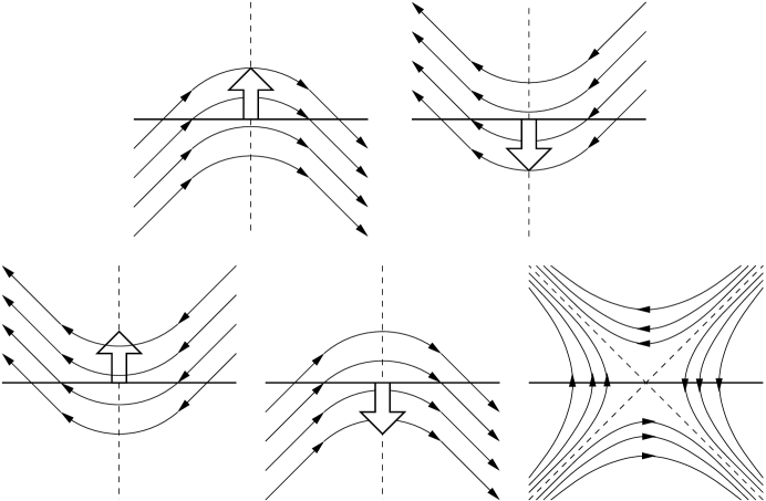
Figure 1: Top row: sketch of field lines (thin, solid) in two possible processes that cause more flux to appear in magnetograms, $\Omega$-loop emergence (left) and U-loop submergence (right), viewed in a plane perpendicular to the polarity inversion line (PIL; vertical, dashed line in all panels). The horizontal solid line represents the magnetogram layer. Near disk center, if the evolution is ideal, then the plasma velocity (fat, white arrows) should produce Doppler shifts along the PIL. Bottom row: Sketches of three possible processes in magnetic flux cancellation: emergence of U-loops (left), submergence of $\Omega$-loops (middle), or reconnective cancellation (right). As with the top row, if the evolution is ideal, then the plasma velocity (fat, white arrows) should produce Doppler shifts along the PIL for emergence or submergence flux (left and middle panels, respectively) near disk center. In principle, processes that increase or decrease total unsigned flux only occur along PILs.

Spruit et al. (1987) proposed that opposite polarities within active regions could be connected by U-loop subsurface extensions, and that flux in these extensions might emerge as weak, “sea-serpent” (undulating) fields between strong field regions, eventually canceling with active region flux via U-loop emergence. Low (2001) proposed a process that also removes most active region flux from the photosphere by the emergence of U-loops. He suggests that the flux rope that forms an active region contains many turns, such that a magnetogram can intersect the flux rope many times after the flux rope has partially emerged, and as the flux rope continues to emerge, much of the flux cancels by U-loop emergence, with successive magnetograms showing less and less flux remaining until little is left. In contrast to these models, van Ballegooijen & Mackay (2007) and van Ballegooijen (2008) constructed numerical models of active region flux systems remaining anchored near the base of the convection zone, with most canceling flux retracting to “repair” the toroidal magnetic field deep in the solar interior.

Spruit et al. (1987) noted that sea-serpent cancellation might occur on small scales. On unobservably small scales, this would produce apparent in situ flux disappearance (Wallenhorst & Howard, 1982; Wallenhorst & Topka, 1982; Gaizauskas et al., 1983). Further, unlike the “self-cancellation” of active region flux modeled by Spruit et al. (1987), Low (2001), and van Ballegooijen & Mackay (2007), active region fields might also cancel with the ubiquitous, small-scale fields of the quiet sun (e.g., Lin & Rimmele 1999, Harvey et al. 2007), including unresolved fields (Sánchez Almeida, 2009). This process would formally remove equal amounts of active-region and quiet-Sun flux from the photosphere, but if the latter were below a given magnetograph’s noise threshold, it would be undetectable, and the active-region flux would have seemed to disappear. While case studies of cancellation have been made, it is unclear how much active region flux cancels on observable scales over a solar cycle. Hence, it is possible that cancellation with quiet-Sun flux is the dominant method of active region flux removal. Moving magnetic features in moat flows around sunspots can explain rates of sunspot flux loss (e.g., Kubo et al. 2008), but much flux in active regions lies outside sunspots, and its disappearance must still be understood.

Because magnetic fields are divergence-free, all field lines (tangent lines of the vector field ${\mathbf{B}}$) form closed loops. (These might be infinitely long, or ergodic, but in any case field lines do not end.) Magnetic flux can therefore only emerge or cancel where magnetic fields are tangent to the photosphere. These loci correspond to normal-field PILs, where the normal magnetic field vanishes and regions of positive and negative flux, where emerging (or submerging) field lines thread the photosphere, are nearby. In our terminology, the appearance (or cancellation) of magnetic flux increases (resp., decreases) the total unsigned magnetic flux at the photosphere.

If the photospheric electric field during cancellation is ideal or nearly so, then measurements of time-averaged Doppler shifts along PILs should be able to distinguish between cancellation via either U-loop emergence or $\Omega$-loop submergence. Lack of a clear Doppler signal while LOS flux cancels would be consistent with reconnective cancellation. We note that the magnetic field along PILs away from disk center in LOS magnetograms can have a component that is normal to the photosphere, implying LOS PILs away from disk center do not exactly correspond to sites of flux appearance (or cancellation). Hence, only Doppler shifts along LOS PILs near disk center can effectively constrain the physical processes at work in cancellation.

Several case studies of Doppler shifts at cancellation sites have been undertaken. Yurchyshyn & Wang (2001) and Bellot Rubio & Beck (2005) reported Doppler shifts consistent with upflows at the cancellation sites they studied, which they interpreted as outflows from reconnective cancellation. Chae et al. (2004) and Iida et al. (2010) found evidence for flux submergence during cancellation. Kubo & Shimizu (2007) studied cancellations along several PILs in ASP magnetograms, and reported mixed Doppler signals, which they interpreted in terms of reconnective cancellation at multiple heights. To determine the rest wavelengths used to compute Doppler velocities, Chae et al. (2004) used quiet-Sun values of line center, while Kubo & Shimizu (2007) and Iida et al. (2010) estimated their rest wavelengths by averaging line centers over their FOVs. As described below, however, these approaches to determining rest wavelengths probably yield biased estimates.

1.3 Biases in Doppler Shifts Along PILs

One factor complicating use of Doppler data both to estimate photospheric electric fields and to constrain dynamics in flux cancellation is inaccuracies in determination of the rest wavelengths of photospheric lines in active regions. Uncertainties in rest wavelength can arise from both instrumental effects (e.g., from thermal variations in components) and biases in analysis techniques. In addition, the gravitational redshift is present (Takeda & Ueno, 2012). Periodicities in magnetic fields estimated by HMI Liu et al. (2012a) on orbital time scales (12 and 24 hr) suggest instrumental effects are present in estimated magnetic fields. It is plausible that similar effects should be present in Doppler signals, a point we revisit below.

Because the position of line center is typically computed from sampling predominantly quiet-Sun regions, where line profiles are systematically shifted blue-ward by the convective blueshift (Dravins et al., 1981; Cavallini et al., 1986; Hathaway, 1992; Asplund & Collet, 2003; Schuck, 2010), Doppler shifts in active regions typically exhibit “pseudo-redshifts.” The blue-ward bias of quiet-Sun line profiles occurs because rising plasma is both (i) brighter than sinking plasma (since rising plasma is hotter) and (ii) occupies a greater fraction of an instrument’s FOV than sinking plasma (since upwelling convective cells are larger than downflow lanes). Consequently, a determination of line center position based upon the statistical properties (e.g., means or medians) of Doppler images (Dopplergrams) is biased by the upward motion of quiet-Sun plasma. Observations and modeling, by, e.g., Gray (2009) and Asplund & Collet (2003), respectively, suggest that the magnitude of this bias can range from a few hundred m sec^-1 to nearly 1 km sec^-1 for various photospheric lines. Because active region magnetic fields inhibit convection (e.g., Welsch et al. 2012), measured line centers in active regions are red-shifted relative to any rest wavelength derived from quiet-Sun Doppler measurements. (Helioseismology requires accurate measurement of changes in Doppler shifts, so is insensitive to errors in determination of the rest wavelength.) P. Scherrer (private communication 2009) has stated that one must account for the convective blueshift to accurately determine Doppler shifts in active regions.

By fitting measured Doppler shifts over the disk with profiles that account for differential rotation, meridional flow, and center-to-limb variations, any overall constant Doppler shift (sometimes referred to as the convective limb shift; Hathaway 1992) can be estimated (Snodgrass, 1984; Hathaway, 1992; Schuck, 2010). This approach, however, has a major physical uncertainty: the physics of the center-to-limb variation in average Doppler shift in the particular spectral line used by HMI (or any other spectral line) involves detailed interactions between height of formation, the height of convective turnover, the variation with viewing angle of the average convective flow speed, and the variation with viewing angle of optical depth (Carlsson et al., 2004; Takeda & Ueno, 2012). We note that diverging flows tangent to the photosphere in granules can, depending upon optical depth in granules at the formation height of the line, produce a convective blueshift toward the limb, because diverging flows on the near sides of granules approach the viewer, while receding flows on the far sides of the granules are at least partially obscured by the optical depth of the granules. This is sketched in Figure 2. Hence, fitting the observed center-to-limb variation in line-center positions does not imply that all bias from convective motions has been determined. In principle, simulations of convection near the photosphere (e.g., Asplund & Collet 2003; Fleck et al. 2011) could be used to characterize the expected center-to-limb variation in line centers, which could then be used to remove the modeled convective blueshift bias (but not any instrumental biases). We are unaware of published comparisons of observed and modeled center-to-limb variations in the HMI spectral line.

Figure 2: Idealized convective motions near the photosphere from center to limb. Thick black arrows represent velocity vectors. Thin black solid lines represent stream lines. Thick dashed line represents optical depth unity, and shows granules’ three-dimensional structure (e.g., Berger et al. 2007; Carlsson et al. 2004). For an observer looking from the top of the figure down, Doppler velocities along lines of sight (thin vertical dashed lines) both at disk center and toward the limb intersect more areas with velocities toward the observer than away. This is one reason that determination of the rest wavelength by averaging (or taking the median) of line center positions over the FOV will result in an estimate biased blue-ward of the true rest wavelength. This analysis ignores the additional factor that upflowing plasma is brighter than downflowing plasma, so the former contributes more to intensity-averaged line profiles.

The goal of this paper is to describe a “magnetic calibration” technique to estimate any spatially uniform bias in measured Doppler velocities. In basic terms, this method estimates such a bias by requiring statistical consistency between two independent measures of changes in flux near LOS-field PILs, the loci where flux emerges and submerges: (1) $\Delta\Phi_{\rm LOS}$, half the change of total unsigned LOS flux near PILs over a time interval $\Delta t$; and (2) $\Delta\Phi_{vBL}$, the amount of transverse flux transported upward or downward across the magnetogram layer over $\Delta t$, computed by summing the Doppler electric field — the product of the Doppler velocity and transverse magnetic field strength — along PILs. This consistency relies upon both Faraday’s law and the assumption of ideal evolution.

The rest of the paper is organized as follows. In the next section, we describe our calibration method in greater detail. We then apply the method to the initial vector magnetogram sequence released by the HMI Team, starting with a description of our preliminary treatment of the data (§3) followed by a step-by-step demonstration of the method (§4) and analysis of its results (§5). We conclude with a brief summary in §6.

2 Calibrating Doppler Shifts with Faraday’s Law

Consider a region of the photosphere where flux is either increasing or decreasing due to appearance or cancellation (by any of the mechanisms discussed above), respectively. In an area $A$ containing flux of one polarity, Faraday’s law and Stokes’ theorem relate the time rate of change of magnetic flux, $\partial\Phi/\partial t$, through $A$ with the integral of the electric field $c{\mathbf{E}}$ projected onto a closed curve $\cal C$ bounding $A$,

$$\frac{\partial\Phi_{A}}{\partial t} = \int dA\,\frac{\partial{\mathbf{B}}}{\partial t}\cdot\,\hat{\mathbf{n}}$$ (5)

$$= -\int dA\,(\nabla\times c{\mathbf{E}})\cdot\,\hat{\mathbf{n}}$$ (6)

$$= -\oint_{\cal C}c{\mathbf{E}}\cdot d{\mathbf{x}}_{\parallel}~{},$$ (7)

where $\,\hat{\mathbf{n}}$ is the unit normal vector on $A$ and $\,\hat{\mathbf{x}}_{\parallel}$ is the tangent vector to ${\cal C}$ oriented to circulate in a right-hand sense (counterclockwise) with respect to $\,\hat{\mathbf{n}}$. This must apply separately to the areas $A_{\pm}$ containing the flux of each polarity.

We restrict ourselves to the case where the flux through areas $A_{\pm}$ changes only due to emergence or cancellation, so flux is only added to or removed from $A_{\pm}$ along the PIL. Hence, the only contribution to the integral of ${\mathbf{E}}$ along $\cal C$ occurs along the PIL,

$$\frac{\partial\Phi_{A}}{\partial t}=-\int_{\rm PIL}c{\mathbf{E}}\cdot d{\mathbf{x}}_{\parallel}~{}.$$ (8)

The time rate of change of flux is therefore equal to the voltage drop along the PIL. This equivalence is exact, without approximation. In real data, however, some PILs might not be observable at a given instrument’s spatial resolution, flux cannot be measured without uncertainties, and flows on the peripheries of $A_{\pm}$ can disperse flux until its density falls below a magnetograph’s sensitivity. In addition, we note that real PILs are often intermittent, and possess complicated spatial structure, motivating our application of this approach with real data, below.

Whether the electric field contains a non-ideal component or not, the rate of ideal transport of magnetic flux across the PIL is given by replacing $c{\mathbf{E}}$ with $-({\mathbf{v}}\times{\mathbf{B}})$ in equation (8),

$$\frac{\partial\Phi_{vBL}}{\partial t}=\int_{\rm PIL}({\mathbf{v}}\times{\mathbf{B}})\cdot d{\mathbf{x}}_{\parallel}~{},$$ (9)

where the subscript $vBL$ denotes that this expression represents the transport of flux across the PIL by plasma flows. We now define a unit vector perpendicular to the PIL, $\,\hat{\mathbf{x}}_{\perp}$, with respect to $\,\hat{\mathbf{n}}$ and $\,\hat{\mathbf{x}}_{\parallel}$,

$$\,\hat{\mathbf{x}}_{\perp}=\,\hat{\mathbf{x}}_{\parallel}\times\,\hat{\mathbf{n}}~{},$$ (10)

which points in the direction of the horizontal gradient of $B_{n}$ evaluated at the PIL (because the PIL is assumed to be a zero contour of $B_{n}$), and $d{\mathbf{x}}_{\parallel}=\,\hat{\mathbf{x}}_{\parallel}dL$. Then

$$\frac{\partial\Phi_{vBL}}{\partial t} = \int_{\rm PIL}dL\,(v_{n}B_{\perp}-v_{\perp}B_{n})$$ (11)

$$= \int_{\rm PIL}dL\,v_{n}B_{\perp}~{},$$ (12)

where ${\mathbf{B}}_{h}$ the field tangent to the surface, $B_{\perp}$ is the component of ${\mathbf{B}}_{h}$ along $\,\hat{\mathbf{x}}_{\perp}$, and the final equality holds because $B_{n}$ vanishes along the PIL.

If the magnetic evolution is ideal, then the rate of change of flux in each area $A_{\pm}$ will match the rate of ideal flux transport across the PIL,

$$\left|\frac{\partial\Phi_{A_{\pm}}}{\partial t}\right| = \left|\frac{\partial\Phi_{vBL}}{\partial t}\right|$$ (13)

$$\left|\int dA_{\pm}\,\frac{\partial{\mathbf{B}}}{\partial t}\cdot\,\hat{\mathbf{n}}\right| = \left|\int_{\rm PIL}dL\,v_{n}B_{\perp}\right|~{},$$ (14)

where $dA_{\pm}$ denotes integration over either polarity (not both). The key point here is that the PIL-integrated rate of transport of horizontal flux by the normal velocity matches the rate of change of normal flux through $A_{\pm}$. Unlike equation (8), this equivalence rests upon the assumption of ideality. (Also, we discuss the effect of filling factors below.) In general, only the unsigned changes in flux match, since both up- and downflows can lead to flux decrease by cancellation (Figure 1, bottom left and center), and both up- and downflows can lead to flux appearance, by either $\Omega$-loop emergence or $U$-loop submergence (Figure 1, top row; and Abbett 2007). Figure 3 sketches emergence of an $\Omega$-loop flux system, one physical situation to which this formalism can be applied.

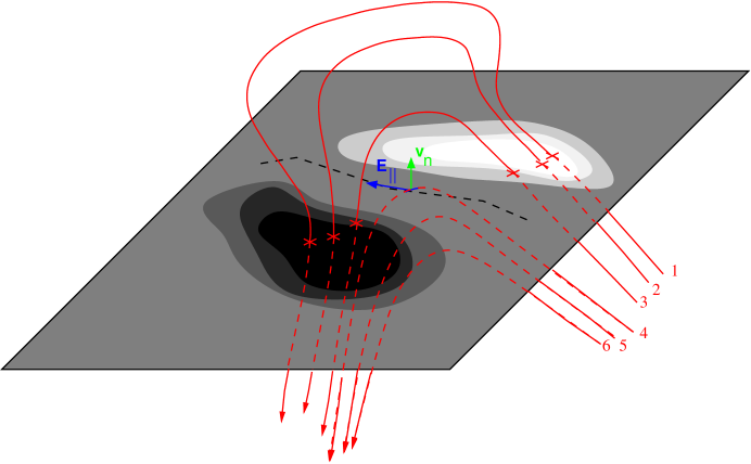
Figure 3: A depiction of ideal flux emergence across the photosphere (gray surface). Magnetic field lines 1,2, and 3 extend from the solar interior (red dashed lines), across the photosphere (red $\times$’s), and out into the outer solar atmosphere (red solid lines). Along a PIL (dashed black line) between regions of positive (white/light shades) and negative (black/dark shades) magnetic flux, a velocity (green vector) normal to the photosphere is driving flux emergence. At the instant depicted, the field line labeled 4 is crossing the photosphere. Additional vertical transport of flux (containing field lines 5 and 6) would cause unsigned flux through the positive and negative flux regions to increase. An ideal electric field (blue vector) parallels the PIL at the emergence site.

We can apply this formalism to PILs of the LOS field near disk center. We require both Dopplergrams, in which the LOS velocity $v_{\rm LOS}$ is measured, and vector magnetograms, in which pixel-averaged flux densities of magnetic components both along the LOS, $B_{\rm LOS}$, and transverse to the LOS, ${\mathbf{B}}_{\rm trs}$, are determined. We approximate the normal vector $\,\hat{\mathbf{n}}$ used above with the unit vector along the LOS, $\,\hat{\mathbf{\ell}}$, replace the exact time derivatives above with finite-difference approximations, and change integrations to summations over pixels in $A_{\pm}$ and along the PIL. Equation (5) then becomes

$$\frac{\Delta\Phi_{\pm}}{\Delta t}=\sum_{\pm}\,(\Delta x)^{2}\frac{B_{LOS}(t_{f})-B_{LOS}(t_{i})}{\Delta t}~{},$$ (15)

where $\Delta x$ is the pixel length, and each sum — there are two, one over each polarity — runs over pixels in the neighborhood of the PIL. (We address identification of PILs and definition of neighborhoods near each PIL below.) Equation (12) then becomes

$$\frac{\Delta\Phi_{vBL}}{\Delta t}=\sum_{\rm PIL}\Delta x\,v_{\rm LOS}B_{\perp}~{},$$ (16)

where the sum runs over PIL pixels, and $B_{\perp}$ now refers to the component of ${\mathbf{B}}_{\rm trs}$ along $\,\hat{\mathbf{x}}_{\perp}$. Equation (14) then becomes, formally,

$$|{\Delta\Phi_{LOS,\pm}}| = |{\Delta\Phi_{vBL}}|$$ (17)

$$\left|\sum_{+\,\,\mbox{or}\,\,-}\,(B_{\rm LOS}(t_{f})-B_{\rm LOS}(t_{i}))\right| = \left|\Delta t\sum_{\rm PIL}\Delta x\,v_{\rm LOS}B_{\perp}\right|~{},$$ (18)

where we have multiplied equations (15) and (16) by $\Delta t$ to deal with changes in flux instead of rates of change in flux, and the sum in the left half of equation (18) runs over the near-PIL neighborhood of one LOS polarity or the other.

Crucially, LOS velocities along PILs are therefore constrained by evolution of nearby LOS flux: over a time interval $\Delta t$, the change in LOS flux in each polarity in the neighborhood of a PIL should match, within methodological uncertainties, the transport of transverse magnetic field by LOS velocities summed along PIL pixels.

As mentioned in the introduction, however, a nonzero bias velocity $v_{0}$ might be present in estimated Doppler velocities from HMI, perhaps due to instrumental effects or the convective blueshift. We define the biased and true Doppler velocities as $v_{\rm LOS}^{\prime}$ and $v_{\rm LOS}$, respectively, which are related via

$$v_{\rm LOS}^{\prime}=v_{\rm LOS}+v_{0}~{}.$$ (19)

We follow the astrophysical convention that receding velocities with respect to the observer — i.e., redshifts — are positive. Then for $v_{0}>0$, the biased Doppler shift is more red than the true Doppler shift. Such an offset in the Doppler velocity would mean that the true rate of flux emergence or submergence is related to the biased rate $\Delta\Phi^{\prime}_{vBL}/\Delta t$ by

$$\frac{\Delta\Phi_{vBL}}{\Delta t} = \sum_{\rm PIL}\Delta x\,v_{\rm LOS}^{\prime}B_{\perp}-\sum_{\rm PIL}\Delta x\,v_{0}B_{\perp}$$ (20)

$$= \frac{\Delta\Phi_{vBL}^{\prime}}{\Delta t}-\frac{\Delta\Phi_{\rm bias}}{\Delta t}~{},$$ (21)

where the bias flux $\Delta\Phi_{\rm bias}$ is due to the bias velocity $v_{0}$,

$$\Delta\Phi_{\rm bias}\equiv v_{0}\Delta t\overline{BL}~{},$$ (22)

and where we define the magnetic length of the PIL as

$$\overline{BL}\equiv\sum_{\rm PIL}(\Delta x)B_{\perp}~{}.$$ (23)

Equation (17) then implies

$$\left|\Delta\Phi_{\rm LOS,\pm}\right|=\left|\Delta\Phi_{vBL}^{\prime}-\Delta\Phi_{\rm bias}\right|~{}.$$ (24)

In the absence of errors, the observed quantities $\Delta\Phi_{\rm LOS}$ and $\Delta\Phi_{vBL}^{\prime}$ enable $\Delta\Phi_{\rm bias}$ to be determined, from which the bias velocity $v_{0}$ can be found via equation (22). Errors are certainly present in these quantities, however, and the evolution also might not be ideal. At this point, however, two key points should be noted:

• First, the rest wavelength of the spectral line used to infer Doppler velocities is a unique, well-defined physical quantity.

• Second, any bias in the rest wavelength should be spatially uniform over the instrument FOV in an individual measurement.

These ideas imply that the set of bias fluxes $\{\Delta\Phi_{\rm bias}\}$ and magnetic lengths $\{\overline{BL}\}$ measured over a set of PILs near disk center can be used to estimate $v_{0}$ statistically, which also enables quantifying uncertainties in the estimate.

It should be noted that, although we derived the flux-matching constraint in equation (18) by considering flux appearance / cancellation, this constraint can determine $v_{0}$ whether or not flux is emerging or submerging. Imagine, for instance, no actual emergence / submergence (i.e., no significant changes in total unsigned LOS flux) were occurring; a nonzero $v_{0}$ would, however, imply spurious emergence / submergence along PILs.

As noted in the introduction, away from disk center, the approximate coincidence between LOS PILs and the radial-field PILs where flux appears or cancels breaks down. While the formalism used here could potentially be developed further to enable analysis of PILs significantly away from disk center, we will restrict our analysis here to PILs near disk center. In Appendix A, we consider pathologies in applying this method to PILs away from disk center.

There are several ways one might estimate the flux changes $\Delta\Phi_{\rm LOS}$ and $\Delta\Phi_{vBL}$ and magnetic length $\overline{BL}$ for each PIL, along with several ways sets of these estimates can be used to estimate $v_{0}$, and thereby remove any bias present in measured Doppler velocities $v_{\rm LOS}^{\prime}$. Accordingly, in the following sections, we demonstrate our approach with actual HMI observations, with several goals in mind: first, to make the method more clear; second, to show that the method can be used with real data; third, to show the method derives physically reasonable values; and fourth, to investigate the extent to which the method depends upon input parameters and is susceptible to errors.

3 HMI Observations

Recently, the HMI Team released a sequence of “cutout” vector magnetograms and Dopplergrams from NOAA AR 11158, from 12-16 Feb. 2011. Members of the HMI Team have put detailed information about this dataset online,, and are preparing a paper describing production of this dataset. This active region was the source of an X2.2 flare on on 2011/02/15, starting in GOES at 01:44, ending at 02:06, and peaking at 01:56. Figure 4 shows the LOS magnetic field in a subregion of the data array near 10:00UT on 2011/02/14.

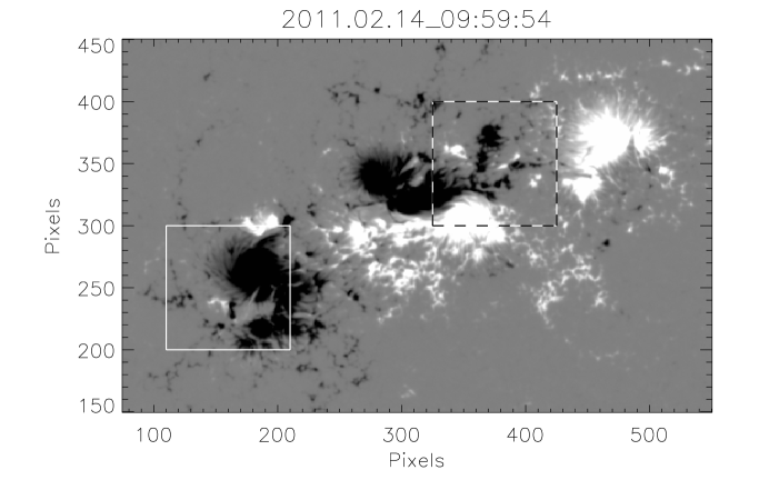
Figure 4: A grayscale image of the LOS magnetic field in AR 11158 near 10:00UT on 2011/02/14 in subregion of the data released by the HMI Team. White/black represent positive/negative LOS flux, respectively. Image saturation is set at $\pm 750$ G. The solid white box outlines a subregion of the FOV shown in Figure 5, and the white/black dashed box outlines the subregion shown in Figure 7.

In this section, we briefly describe procedures that we undertook to prepare this data prior to applying our calibration procedure.

After downloading the FITS data files, several processing steps were required, which we describe here. Because the read_sdo.pro IDL procedure did not (at the time of this writing) properly handle pixels set to the BLANK value in the FITS headers, we used the fitsio_read_image.pro procedure to read in the data.

3.1 Cropping

To reduce the full dataset to a more manageable size, we focus on a subset of the full five-day sequence. To study photospheric magnetic evolution prior to the X flare, and to baseline this evolution against post-flare evolution, we retain about 72 hours of data, from midnight at the start of the 13th until midnight at the end of the 15th, inclusive of endpoints. Given the 12-minute cadence, the resulting time series consists of 361 time steps. The active region was at S19E11 at 00:30UT on 2011/02/13 and S21W27 at 00:30UT on 2011/02/16. Pixels lacking data near the edges of the cutout FOV, from artifacts of the cutout process, were cropped: columns [0 – 24] and rows [0 – 5] were removed for all steps.

3.2 Removing SDO Motion and Solar Rotation

Next, Doppler velocities were corrected for spacecraft motion. Due to SDO’s geosynchronous orbit, its velocity along the radial, Sun-observer line can be large, of order $\pm$ 5 km s^-1. Also, because the Earth is orbiting westward about the Sun, and SDO orbits Earth, there is a significant projection of SDO’s westward motion onto lines of sight to many pixels. In addition, there is a nonzero component of SDO’s northward velocity onto the LOS. While the radial component is larger than the W and N components, the latter can be significant — a few tens of m s^-1 or more. Accordingly, the spacecraft velocity was projected onto the LOS to each pixel — in the small-angle approximation — and subtracted off the measured Doppler velocities. Then Stonyhurst latitudes and longitudes of each pixel (accounting for the solar $B$ and $P$ angles) were computed to correct Doppler velocities for solar rotation, using the “magnetic/ 2-day lag” rotation rate found by Snodgrass (1983), for which

$$\omega_{\rm rot} = A+B\sin(\tilde{\theta})^{2}+C\sin(\tilde{\theta})^{4}$$ (25)

$$A = 2.902$$ (26)

$$B = -0.464$$ (27)

$$C = -0.328~{},$$ (28)

where $\omega_{\rm rot}$ is the photospheric rotation rate, $\tilde{\theta}$ is latitude, and $A,B$, and $C$ are in microrad s^-1. Accurate correction for rotation prior to application of our calibration procedure is not necessary; but without removing it, the bias velocity estimates will include (and could be dominated by) the Doppler shift from rotation.

We also note that the Doppler signal from helioseismic $p$-mode oscillations, which have a peak in power at frequencies near 1/300 Hz, could introduce non-convective signals into the 720-second cadence Dopplergrams. While individual mode amplitudes are on the order of a few tens of cm s^-1, the overall motion due to the superposed modes can be 500 m s^-1 or more, which is comparable to convective motions. In practice, however, HMI’s 720-second Dopplergrams are created by averaging higher-cadence filtergrams with a cosine-apodized, 1215-second boxcar Liu et al. (2012b) with a full width at half maximum of 720 seconds (Schou 2012, private communication). This effectively acts as a filter, which would reduce a random-phase sinusoidal signal with period of 300 s and amplitude of 500 m s^-1 to an averaged value of less than 20 m s^-1 (less than the noise level of HMI Dopplergrams).

3.3 Removing Azimuth Reversals

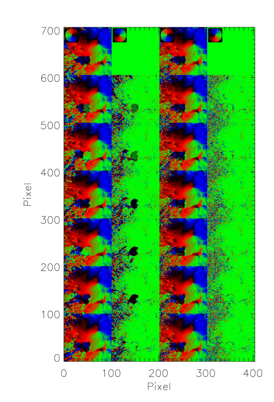
Figure 5: We applied a filtering procedure to remove back-and-forth flips in azimuth, which are likely due to frame-to-frame inconsistencies in ambiguity resolution. From left to right, 1st column: 100 $\times$ 100 pixel maps of transverse-field azimuths (color wheel in top panel) from the solid white box in Figure 4 from seven successive vector magnetograms (separated by 12 minutes), starting at 10:00UT on 2011/02/14. Time increases down. 2nd column: Difference in azimuth between current and previous maps (note different color wheel in top panel). Initial difference map is arbitrarily set to zero. 3rd column: Filtered versions of the azimuth maps in the 1st column, in which continuity in azimuths has been imposed (color wheel in top panel). 4th column: Difference in azimuth between current and previous filtered maps (color wheel in top panel). Initial difference map is arbitrarily set to zero. Back-and-forth flips in many pixels have been removed.

Accurate estimation of electric fields by PTD (or, really, any method) requires that changes in ${\mathbf{B}}$ between magnetograms arise from physical processes on the Sun, as opposed to artifacts of the measurement process. Hence, any spurious changes in the measured field, where they can be identified, should be removed.

We noticed that in successive images of the transverse-field azimuths, the inferred azimuths in some regions flip by nearly 180 degrees from one frame to the next, as would be expected from errors in resolving the 180-ambiguity. The seven successive frames (12 min. apart) in the left column of Figure 5 show an example of this effect, with time increasing downward. The area shown corresponds to that in the solid white box in Figure 4, and the initial frame corresponds to that in Figure 4. Azimuths range over [0,360] degrees. The next column shows maps of the angular difference (the interior angle) between the current and previous azimuths. Differences in azimuths range from [-180,180] degrees (note the rotated color wheel in the top panel). The black patches in rows 4 – 6 of this column correspond to a region in which azimuths flip by nearly 180^∘ in a region from one frame to the next. The checkerboard pattern in the same region in rows 2 – 3 of this column implies a spatially alternating pattern of 180^∘ azimuth flips, and probably arises from lack of convergence in the simulated annealing algorithm used to infer the azimuths (Leka et al., 2009). Also, the red-and-blue, speckled regions toward the left side of each frame in this column exhibit rapid spatial variations in azimuth changes. These speckled regions correspond to areas with relatively weak field strength ($B<200$ G), where azimuth determinations could be more problematic than in strong-field regions.

Interpreting frame-to-frame azimuth flips over finite regions as spurious, we seek to identify and remove these artifacts. Our goal is to automate detection of such flips, and our basic approach is to identify suspicious changes in azimuth, which we envision as “top hats” (or inverted top hats) in the running differences of azimuths in individual pixels: large, positive (or negative) jumps in azimuth for one time step, followed by reversals to the pre-jump level at the next step. The actual patching is simpler: we add 180 degrees to the azimuth, and output the flipped data modulo 360 degrees.

We tried more than one approach to detecting and correcting spurious azimuth changes before finding one that we think works well. To save other researchers from repeating our efforts, we now describe, in detail, both our failed approach and the approach we found worked best.

In our initial, unsuccessful approach, we simply identified all pixels with unsigned changes in azimuth from frame $(i-1)$ to frame $i$ above a given threshold (we tried, e.g., 120, 135, 150, and 170 degrees), and flipping these in frame $i$. The updated frame $i$ was then used as a reference for finding large changes in frame $(i+1)$. Using this approach, once a pixel is flipped, its new state tends to be propagated forward in time. But legitimate magnetic evolution can cause this state to be incorrect, leading to spatially isolated pixels that differ from their neighbors. This contradicts a central tenet of the original ambiguity resolution procedure: currents should be minimized. Further, the number and spatial arrangement of problematic pixels appears to depend strongly on threshold.

The best approach we found is to flip azimuths only in pixels where both: (i) the jump in azimuth was larger than 120^∘ between frames; and (ii) the jump in azimuth increased the time-averaged, unsigned changes in azimuth over a the set of frames within $\pm N$ steps of a given frame. Use of a range of images on either side of the $i$-th image is necessary to capture the essential character of a top hat: a large change, followed by a reversal. (A large azimuth change from one frame to the next, by itself, might be legitimate — e.g., by horizontal advection of a region with a spatial transverse field reversal.) We determined suspicious flips by comparing means of two arrays of $2N$ azimuth differences: (1) unsigned differences between the azimuths at frame $i$ and azimuths in $\pm N$ neighboring frames in time, $[i-N:i-1]$ and $[i+1:i+N]$; and (2) unsigned differences between the flipped azimuths (hypothetical data, with all pixels’ azimuths flipped) at frame $i$ with actual azimuths in $\pm N$ neighboring frames in time, $[i-N:i-1]$ and $[i+1:i+N]$. Pixels for which flipping would decrease the mean, unsigned, frame-to-frame angular differences are then flipped.

We call frames in which azimuths have been flipped filtered. Filtered azimuths are used for past frames, $[i-N:i-1],$ while unfiltered azimuths are used for future frames $[i+1:i+N],$ so this approach is not time-symmetric. This approach should be able to deal with top hats that are $N$ steps wide, but not wider. We tried both $N=4$ and $N=2$, and show results with $N$ = 2 here. Using $N=4$ results in 2–5% fewer flips in a given frame, so is slightly more restrictive. We did not, however, see much difference between results from $N=2$ and $N=4$ in strong-field regions, so most differences are probably in weak-field regions where inference of the direction of transverse fields is less reliable anyway.

The third column from left in Figure 5 shows filtered data from the same seven successive frames as in the left-most column, with suspicious changes in azimuths identified by our approach flipped by 180^∘. The right-most column shows maps of the angular difference between the current and previous azimuths (note the rotated color wheel in the top panel) from the third column. The checkerboard and black patches visible in the second column are not present in this column. Also, changes in azimuths in the red-and-blue, speckled regions on the left sides of each frame are not as large in this column as in the second column. This suggests our approach decreases fluctuations of azimuths in weak-field regions, too.

4 Demonstration of Electromagnetic Calibration

We now seek to quantify any bias velocity in the Doppler velocity measurements. Since this will require associating pixel values in successive frames (e.g., in equation 15), we first co-aligned the plane-of-sky (POS) Dopplergram, field strength, and inclination arrays. We used the $B_{\rm LOS}$ arrays as the reference observations, since structures in $B_{\rm LOS}$ are long-lived (e.g., Welsch et al. 2012). Whole-frame shifts between each $B_{\rm LOS}$ array were determined to sub-pixel accuracy using Fourier cross-correlation, and the data arrays were shifted accordingly via Fourier interpolation. Instead of wrapping data across image edges, due to the assumed periodicity in the Fourier method, data shifted out of the image field of view were zeroed out. Interpolated field inclinations outside [0,180] were capped at these values. We then used the co-aligned inclinations and field strengths to derive co-aligned LOS and transverse fields.

Our calibration method requires several additional tasks: identifying PILs of the LOS field; quantifying changes in LOS magnetic flux near those PILs; summing transverse fields $B_{\rm trs}$ and Doppler velocities $v_{\rm LOS}^{\prime}$ along identified PILs; and statistically estimating any offset $v_{0}$ in these Doppler velocities.

4.1 Identification of PILs

The first step in our approach is to use an automated algorithm to identify PILs in LOS magnetograms. Our procedure creates masks of each polarity for pixels with $|B_{\rm LOS}|$ above a field strength threshold of $B_{\rm thr}$, dilates each mask by one pixel, and finds all areas where the dilated masks overlap (see Schrijver 2007; Welsch & Li 2008). The threshold field is the only input parameter in PIL identification procedure; here, we use $B_{\rm thr}=50$ Mx cm^-2, ensuring that we identify relatively strong fields in close proximity. This approach identifies structures 1–3 pixels wide, which we erode into single-pixel-width lines with IDL’s morph_thin.pro procedure. We define the resulting pixels to be PIL pixels. In Figure 6, we show identified PIL pixels, color-coded by (possibly biased) Doppler velocity $v_{\rm LOS}^{\prime}$, in a close-up view of the LOS magnetic field at the time step when AR 11158 was closest to disk center.

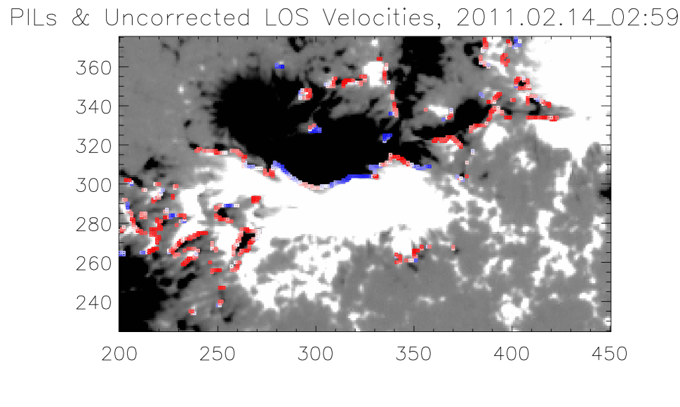
Figure 6: Grayscale image shows a zoomed-in view of $B_{\rm LOS}$, with PIL pixels superimposed and color-coded by (possibly biased) Doppler velocity $v_{\rm LOS}^{\prime}$. Grayscale saturation is set to 100 Mx cm^-2, and the velocity saturation is set to $\pm$ 250 m sec^-1. Note the predominance of redhsifted PILs.

In this sub-region of the full active region, $N_{\rm PIL}=98$ PILs were identified. Most of the Doppler signals along PILs appear redshifted. These are almost certainly pseudo-redshifts, arising from the Doppler zero-point being defined to be blue-ward of the true rest wavelength for photospheric plasma with no LOS velocity. The velocity zero point for HMI is derived from the median of Doppler velocities within 90% of the solar radius over 24 hours (Y. Liu & S. Couvidat, private communication, 2011). This implies contributions from quiet-Sun (and therefore strongly convecting) plasma dominate the median, and probably bias the zero-point.

4.2 Flux Changes Near PILs

Having identified PILs at a given time $t_{0}$, our second step is to estimate the set of changes of LOS flux $\{\Delta\Phi_{\rm LOS}\}$ near all PILs over the $\Delta t=24$ minutes between the two LOS magnetograms observed $\pm 12$ minutes from the magnetogram at $t_{0}$. To do so, for each PIL we create a binary map of that PIL’s pixels, then apply IDL’s dilate.pro procedure with a $(d\times d)$ matrix of 1’s to the binary map to define that PIL’s “neighborhood mask.” The dilation parameter $d$ is the only other free parameter in our method. While granular flows have speeds on the order of $\sim 1$ km sec^-1, such flows are short-lived, with lifetimes of $\sim 5$ min. Over $\Delta t=24$ min, therefore, displacements of fluxes tend to be consistent with lower averaged speeds, on the order of $\sim 0.5$ km sec^-1 or less (see, e.g., Fig. 13 of Welsch et al. 2012). Given the HMI pixel size $\Delta x\simeq 0.5\arcsec\simeq 360$ km near disk center, magnetic flux should not move by more than about two pixels over $\Delta t=24$ min. Here, we use $d=7$ — that is, dilation by $\pm 3$ pixels in all directions — although we have explored other choices (see below). (As Démoulin & Berger (2003) have pointed out, emerging fields that are strongly inclined with respect to the LOS could have very high apparent speeds, implying displacements that would exceed our 3-pixel dilation. Excessive dilation, however, risks incorporating changes in flux that are unrelated to emergence / submergence in PIL neighborhoods.) Next, we multiply the two co-aligned LOS magnetograms from $\pm 12$ minutes by this neighborhood mask and sum the unsigned flux in each product, then difference these summed fluxes. Because this counts LOS flux changes in both polarities, we divide the result by two to estimate $\Delta\Phi_{\rm LOS}$ over $\Delta t=24$ minutes.

It should be noted that converging or diverging horizontal flows unrelated to emergence/ submergence at each PIL can transport “background” flux into the neighborhood of a PIL, and near-PIL flux out of this neighborhood, in some cases dominating our estimates of the change in LOS flux due to emergence or submergence along the PIL. Hence, the computed rate of change in LOS flux along an individual PIL is subject to large errors. Identifying collections of like-polarity pixels as “features” and tracking their evolution (DeForest et al., 2007; Welsch et al., 2011) might be one way to better account for fluctuations in LOS flux due to flux concentration / dispersal (Lamb et al., 2008). Assuming the contributions from converging and diverging flows cancel in the aggregate over many PILs, the statistical properties of changes in LOS fluxes along a set of PILs are more robust to such errors, and therefore more useful for our purposes.

Our third step is to compute, for each PIL, the corresponding expected flux change from the (assumed biased) Doppler signal, $\Delta\Phi_{vBL}^{\prime}$, and magnetic length, $\overline{BL}$. Since the expressions derived for these quantities (equations 18 and 23) in §2 refer to the component of the transverse magnetic field perpendicular to the PIL, we investigated the angle of the transverse magnetic field along PILs in our dataset.

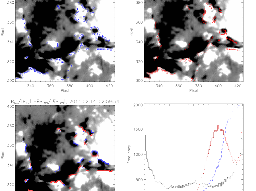
Figure 7: Top left: Unit vectors normal $\,\hat{\mathbf{x}}_{\perp}$ to PILs, along the gradient in $B_{\rm LOS}$ along each PIL in a small subregion of the full FOV. Grayscale background shows $B_{\rm LOS}$, with saturation at $\pm 100$ Mx cm^-2. Top right: Unit vectors $\,\hat{\mathbf{b}}_{\rm trs}$ parallel to ${\mathbf{B}}_{\rm trs}$ along PILs in the same FOV. Bottom left: Color-coded dot product of $\,\hat{\mathbf{x}}_{\perp}\cdot\,\hat{\mathbf{b}}_{\rm trs}\equiv\cos\chi$, with red positive (“inverse” polarity) and saturation set to 0.866, corresponding to 30^∘. The component of ${\mathbf{B}}_{\rm trs}$ perpendicular to each PIL is homogeneous along many PILs. Bottom right: Distributions of PIL-averaged $\cos\chi$ (black), $|\sin\chi|$ (red), and $|\cos\chi|$ (blue), where $\chi$ is the angle between $\,\hat{\mathbf{x}}_{\perp}$ and $\,\hat{\mathbf{b}}_{\rm trs}$. Fields tend to point across (not along) most PILs.

Figure 7 illustrates the geometry of the transverse field along several PILs. The upper-left panel shows unit vectors $\,\hat{\mathbf{x}}_{\perp}$ perpendicular to the PIL, determined from the gradient of $B_{\rm LOS}$ evaluated at PIL pixels. The upper-right panel shows unit vectors $\,\hat{\mathbf{b}}_{\rm trs}$ along ${\mathbf{B}}_{\rm trs}$, evaluated at PIL pixels. Note the predominance of unit vectors $\,\hat{\mathbf{b}}_{\rm trs}$ pointing toward the bottom of the FOV: this coherence might be spurious, and could arise if the minimization of currents by the ambiguity resolution algorithm introduces artificial, large-scale correlations in azimuths. Color coding in the bottom-left panel shows the cosine of the angle $\chi$ between these unit vectors — their dot product, $\,\hat{\mathbf{x}}_{\perp}\cdot\,\hat{\mathbf{b}}_{\rm trs}$ — with red positive, and the saturation level set to $\pm 0.866$. (The sign of the angle $\chi$ is defined such that the angle between $\,\hat{\mathbf{x}}_{\perp}$ and $\,\hat{\mathbf{x}}_{\parallel}$ is +90^∘; see equation 10.) Fields along PILs evidently exhibit components in both the “normal” (positive-to-negative; blue) and “inverse” (negative-to-positive; red) directions (Martens & Zwaan, 2001) perpendicular to the PIL. For each PIL, the mean (PIL-averaged) signed and unsigned $\cos(\chi)$ and unsigned $\sin(\chi)$ can be computed; the bottom-right panel shows the distributions of these averages for all PILs in our dataset. The peaks at -1 and 1 for the signed $\cos(\chi)$ and around 0.5 for $|\sin(\chi)|$ imply that the average field of many PILs: (i) is spatially coherent; and (ii) tends to point primarily across (not along) the PIL.

As with changes in LOS flux near PILs — which can arise from converging or diverging flows unrelated to emergence / submergence — some component of Doppler velocities along identified PILs might be unrelated to emergence / submergence. Slight inaccuracies in PIL identification, for instance, could lead us to improperly include flows along the magnetic field (siphon flows) in our flux transport rates. Also, filling factors — due to scattered light within the HMI instrument, or imaged emission from unresolved, unmagnetized plasma, or both — could bias the estimated flux transport rate in a given pixel (and contributions from either would plausibly tend to be blue-shifted). Hence, as with changes in LOS flux near PILs, the inferred rate of transport of transverse flux along an individual PIL is subject to large errors. Again, the statistical properties of flux transport rates along the aggregated collection PILs should be more robust to error, and therefore more useful for quantifying the pseudo-redshift.

We have also investigated making the simplifying replacement $B_{\perp}\rightarrow B_{\rm trs}$ when computing $\Delta\Phi_{vBL}$ and $\overline{BL}$. Physically, one can justify this approximation by noting that the footpoints of fields with components tangent to the PIL must still thread the photosphere somewhere, if not directly across the PIL, as would be the case for no magnetic component tangent to the PIL. We will show results computed both ways, using either $B_{\perp}$ or $B_{\rm trs}$ at each PIL pixel, but unless otherwise stated, results shown below are derived using $B_{\rm trs}$. As will be seen, this did not drastically change the estimates of bias velocities $v_{0}$, although quantities derived using $B_{\perp}$ were substantially noisier. We also note that using $B_{\rm trs}$ makes the bias estimation technique independent of ambiguity resolution.

4.3 Estimation of Bias Velocities

Finally, we can estimate any bias velocity present. We first difference $\Delta\Phi_{\rm LOS}-\Delta\Phi_{vBL}^{\prime}$ on each PIL to compute the set of bias fluxes $\{\Delta\Phi_{\rm bias}\}$ from all PILs. We must then estimate the coefficient $v_{0}$ from the ratios of $\{\Delta\Phi_{\rm bias}\}$ to $\{\Delta t\overline{BL}\}$.

In the data, errors are present in both measured quantities. Before estimates of typical uncertainties were published by the HMI team, we adopted uniform uncertainties of 20 m/s for the Doppler velocities, 25 Mx cm^-2 for $B_{\rm LOS}$, and 90 Mx cm^-2 for $B_{\rm trs}$. This value for the Doppler uncertainty is consistent with expected near-disk-center noise levels reported by Schou et al. (2012). The value for noise in $B_{\rm LOS}$ is significantly larger than the HMI Team’s since-published estimate the uncertainty of $\sim 6$ Mx cm^-2 in 720-second data (e.g., Liu et al. 2012a), while the value for $B_{\rm trs}$ is probably closer to the HMI Team’s estimate of noise in the transverse component on the order of $10^{2}$ Mx cm^-2 (Sun et al., 2012).

We estimate $v_{0}$ and its uncertainty by analyzing the the set of ratios $\{\Delta\Phi_{\rm bias}/(\Delta t\overline{BL})\}$ over a subset of identified PILs. Based upon both our prior knowledge that the convective blueshift biases the median-derived estimate of the rest wavelength in HMI Doppler data blue-ward, and the predominance of redshifted PILs in Figure 6, we expect that the biased PIL velocities are more red than the true velocities. Recalling that we use the astrophysical convention that redshifts correspond to positive velocities with respect to the observer, the bias velocity $v_{0}$ should be positive.

Not all bias fluxes, however, are consistent with a positive bias velocity. This is not obvious from equation (24), since it deals with absolute values. Consequently, we now consider the different possibilities for the relative sizes of $\Delta\Phi_{\rm LOS},\Delta\Phi_{vBL}^{\prime}$ and $\Delta\Phi_{\rm bias}$. A positive $v_{0}$ is consistent with PILs that obey either

$$\Delta\Phi_{vBL}^{\prime}>|\Delta\Phi_{\rm LOS}|$$ (29)

or

$$-|\Delta\Phi_{\rm LOS}|<\Delta\Phi_{vBL}^{\prime}<0~{},$$ (30)

since the correction to $\Delta\Phi_{vBL}^{\prime}$ is $-\Delta\Phi_{\rm bias}^{\prime}=-v_{0}\Delta t\overline{BL}$. For PILs that obey either

$$|\Delta\Phi_{\rm LOS}|>\Delta\Phi_{vBL}^{\prime}>0$$ (31)

or

$$\Delta\Phi_{vBL}^{\prime}<-|\Delta\Phi_{\rm LOS}|<0~{},$$ (32)

however, $v_{0}$ would have to be negative to improve agreement between the flux changes.

What fraction of PILs are consistent with a positive bias velocity $v_{0}$? Of the $\sim$50,000 PILs identified in the full dataset (with $B_{\rm thr}=50$ Mx cm^-2), 73.8% and 5.7% were consistent with equation (29) and (30), respectively, and 13.9% and 6.6% obeyed equations (31) and (32), respectively. Consequently, $\sim$80% of PILs are consistent with a positive bias velocity.

In Figure 8, we show the distribution of bias fluxes for all PILs at all time steps. (In any single time step, there are $\sim 140$ PILs in our FOV, too few to form a continuous distribution.) The distribution is strongly skewed toward positive bias fluxes. We consider PILs matching either (31) or (32) to be pathological, which we attribute to “noise,” primarily systematic errors in our estimates of the fluxes. (Errors from our assumed uncertainties in the underlying magnetic and Doppler data would be $3\times 10^{16}$ Mx per pixel or less.)

This distribution of bias fluxes can be used to quantify uncertainties in the bias flux.

Figure 8: Dashed line shows the total distribution of bias fluxes for all PILs at all time steps, which is clearly skewed toward the positive. Mirroring the negative bias flux values across zero and fitting the result with a Gaussian (thin solid) enables an empirical estimate of noise in the bias flux from the fitted width, $3.75\times 10^{17}$ Mx. Subtracting the fit from the total distribution of bias fluxes leaves the residual distribution (thick solid) of bias fluxes above the noise level.

Mirroring the negative bias flux values across zero and fitting the result with a Gaussian enables an empirical estimate of noise in the bias flux from the fitted width, $3.75\times 10^{17}$ Mx. Following the same procedure but using $B_{\perp}$ instead of $B_{\rm trs}$ to compute $\Delta\Phi_{vBL}^{\prime}$ results in a fitted width of $5\times 10^{17}$ Mx, reflecting greater uncertainty in estimates of this flux. These define thresholds in the bias flux: estimates of bias fluxes smaller than these levels fall within our (systematic) uncertainties.

Subtracting the fit from the total distribution of bias fluxes leaves the residual distribution of bias fluxes above our uncertainty level. At each step, we computed separate estimates of the bias velocity from both the full set of PILs and just the subset of PILs with bias fluxes more positive than these estimates of the threshold bias fluxes. Not surprisingly, estimates of $v_{0}$ using only PILs with bias fluxes above these thresholds — which we refer to as the “high-bias” subset of PILs — were substantially higher (as shown below) than estimates derived using all PILs. We view use of all PILs as more conservative, so results shown below are derived from all PILs, unless explicitly stated otherwise.

5 Results & Analysis

In Figure 9, we show sorted values of the set $\{v_{0}\}=\{\Delta\Phi_{\rm bias}/(\Delta t\overline{BL})\}$ from all PILs, scaled to units of m/s, derived from three successive magnetogram triplets when AR 11158 was close to the central meridian. It is clear that most values fall well above zero (the lower, dotted line in each plot; recall that we define redshifts as positive). This is entirely consistent with the predominance of redshifts in Figure 6. The means and standard errors in the estimates are $101\pm 17$ m/s, $126\pm 18$ m/s, and $138\pm 16$ m/s, respectively; the means are plotted as horizontal solid lines. Medians are the dashed horizontal lines in each plot (indistinguishable from the mean in the bottom plot). We use the standard error in the estimate (standard deviation divided by $\sqrt{N_{\rm PIL}}$) as a measure of uncertainty since each estimate is a measurement of the same number, $v_{0}$, although we do not know if the errors are Gaussian. Only $\sim$ 45% of error bars are consistent with the average $v_{0}$ in each plot. This suggests either: (1) that our error estimates are too low, perhaps due to our neglect of systematic errors (e.g., in definitions of PIL and their neighborhoods, and in quantifying magnetic fields along PILs); or (2) that electric fields along PILs are in some cases inconsistent with the ideal electric field assumed in equation (3).

Figure 9: Sorted values of the set of bias velocities, $\{v_{0}\}=\{\Delta\Phi_{\rm bias}/(\Delta t\overline{BL})\}$ from all PILs, (in m/s) and estimated errors for each PIL (with the astrophysical convention of positive redshift), from three successive (and partially overlapping) magnetogram triplets. The lower thin dotted line shows the (uncalibrated) zero Doppler velocity. Solid and dashed horizontal lines show average and median bias velocities. The magnitudes of the estimated bias velocities are $101\pm 17$ m/s, $126\pm 18$ m/s, and $138\pm 16$ m/s. Only about $\sim 45$% of error bars are consistent with each average velocity, suggesting our error estimates are too low, or the ideal assumption is invalid. Nonetheless, our results are consistent with the predominance of redshifts in Figure 6, and indicate pseudo-redshifts are present.

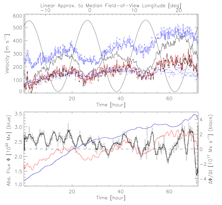
Figure 10: Top: Values for the bias velocity $v_{0}$ for different approaches and parameters used to determine changes in flux near PILs. The median of all PILs, using $B_{\rm trs}$, dilation parameter $d=5$ pixels, and LOS field strength significance threshold $B_{\rm thr}=50$ Mx cm^-2 gives the solid red line. Error bars, omitted for clarity, are on the order of the fluctuations between successive estimates. With the same parameters, but using $B_{\perp}$, the dashed red line results. The solid and dashed blue lines correspond to estimates using the same approaches and parameters as each red line, respectively, but from averaging over only high-bias PILs (see text). The dashed, thick black line (which coincides closely with the red lines) shows the bias velocity using $B_{\rm trs}$, but $d=7$, keeping $B_{\rm thr}=50$ Mx cm^-2. The blue dash marks show the bias velocity using $d=5$, with $B_{\rm thr}=25$ Mx cm^-2. The solid black jagged line shows an empirical estimate of $v_{0}$: the median of Doppler velocity along all PIL pixels identified with the $50$ Mx cm^-2 threshold, which ignores the flux-emergence constraint in equation (18). The smooth, sinusoidal solid line shows 1/10th of the radial component of the spacecraft Doppler velocity, offset by +250 m s^-1 to fit on the plot. Bottom: Total unsigned radial flux (blue) and the raw and smoothed finite-difference time rate of change in that flux (thin gray and thick black, respectively), which is positive when new flux is emerging. Variations in the rate of change of flux are weakly correlated with the smoothed, de-meaned, and scaled bias velocity estimate (red) derived using all PILs, with $d=5$ and $B_{\rm thr}=50$ Mx.

In the top panel of Figure 10 we plot estimates of $v_{0}$ versus time, for different approaches — using either $B_{\rm trs}$ or $B_{\perp}$, and either all PILs or only high-bias PILs — along with different choices for the two parameters in our method, the threshold LOS field strength $B_{\rm thr}$ (25 or 50 Mx cm^-2) that defines significance in identifying PILs, and the dilation parameter $d$ (5 or 7) that defines the neighborhood near each PIL over which changes in LOS flux with time are computed. Estimates made from the median $v_{0}$ from all PILs, with $B_{\rm thr}=50$ Mx cm^-2 and $d=5$ using either $B_{\rm trs}$ or $B_{\perp}$ (red, solid and dashed, respectively) are very similar. (We use medians instead of averages here because some estimates in the full set of PILs made using $B_{\perp}$ are pathologically noisy.) The blue lines are from averaging only high-bias PILs, using either $B_{\rm trs}$ or $B_{\perp}$ (solid and dashed, respectively), and also agree closely. Using $B_{\rm trs}$, increasing $d$ to 7, with $B_{\rm thr}=50$ Mx cm^-2, gives the thick, black dashed line (which closely follows the red lines); decreasing $B_{\rm thr}$ to $25$ Mx cm^-2, with $d=5$, gives the blue dash marks (which are also close to the red lines). Together, these suggest that results are not strongly affected by varying $d$ slightly, or using $B_{\rm trs}$ versus $B_{\perp}$, although estimates of $v_{0}$ from high-bias-flux PILs are systematically higher. We note that the less restrictive threshold flux density, $B_{\rm thr}=25$ Mx cm^-2, resulted in somewhat lower estimated bias velocities, especially toward the end of the run. This might be because PILs in weaker-field regions, which should be more strongly convecting, were included when the lower threshold was used.

The HMI Team’s estimate of the 1$\sigma$ noise in $B_{\rm LOS}$ is about $6$ Mx cm^-2, so the $50$ Mx cm^-2 threshold corresponds to about 8 standard deviations. With $B_{\rm thr}=50$ Mx cm^-2 and $d=5$, the standard deviation between the $i$-th bias estimate made using $B_{\rm trs}$, and a 5-step (1-hr.) running average was 18 m/s, near the noise level of the Dopplergrams. Standard errors in the mean (SEM) were computed using uncertainties assumed above; the average SEM for this series was 22 m s^-1. The consistency of the $v_{0}$ estimates on hour-long time scales is evidence of robustness in our estimates. Variation of $v_{0}$ on time scales longer than few hours is evidence that calibration of the Doppler shifts in time is necessary, as the estimated bias velocity is not constant. For comparison with the phase of SDO’s orbit, we also plot the radial component of spacecraft velocity, rescaled and shifted in the vertical direction (but not in time), in the sinusoidal, black, solid line.

The solid, black, jagged line shows an empirical estimate of $v_{0}$: the median of Doppler velocities along all PIL pixels at each step, identified with the $50$ Mx cm^-2 threshold. This estimate is relatively simple to determine: one only needs to identify PILs of the LOS field, then take the median Doppler velocity on all PIL pixels. This approach, however, ignores the flux-matching constraint in equation (18), and therefore could be biased by a strong episode of flux emergence (or submergence).

A trend in each curve with longitude (upper scale, Figure 10) can be noted, of about 5 m s^-1 deg^-1 for the curves shown. In terms of an error in our assumed rotation rate, this corresponds to $\sim 0.45\mu$rad s^-1, a significant fraction of the $A$ coefficient in equation (25). We note that accurate compensation for the rotation rate prior to applying our method is not required: it can also be applied even if the rotational Doppler shift has not been removed, although the derived bias velocity will then include both rotational and convective shifts.

A more likely explanation for the trend is contamination by Evershed flows on “false” PILs in the LOS field of limb-ward penumbrae. Such artifacts might be ameliorated by only including bias velocity estimates from LOS PILs that are near radial-field PILs.

All of our estimates of the bias velocity $v_{0}$ are positive, although there is a significant spread in the estimates, which range from 50 – 500 m s^-1, with variations in both time (and therefore longitude) and from method and parameter selection. We will compare the physical implications of the differing estimates below.

Could an episode of strong flux emergence somehow influence our estimate of the bias velocity? In principle, the flux-matching constraint in equation (18) should make our approach insensitive to the rate of flux increase or decrease: changes in LOS flux and the transport of flux along the LOS should be consistent, regardless of emergence / submergence rates. Nonetheless, could systematic errors in our approach make our calibration method susceptible to bias during episodes of strong emergence? We investigate this possibility in Figure 10’s bottom panel, which shows the total unsigned radial flux in pixels with absolute radial flux density above 50 Mx cm^-2, and the raw and smoothed (using a five-step boxcar average) finite-difference time rate of change in that flux, which is positive when flux is emerging. The smoothed, de-meaned, and rescaled bias velocity derived from all PILs with $B_{\rm thr}=50$ Mx cm^-2 and $d=5$ is also plotted (red line). Although variations in the rate of change of flux do not appear to strongly influence the bias velocity estimates, we find a weak correlation ($\sim 0.2$) between these time series. A scatter plot, in Figure 11, confirms that the dependence is weak. Nonetheless, we ran a total-least squares linear fit to quantify the dependence, which gives a slope of -11 m s^-1 (10¹⁷ Mx s^-1)^-1, implying that typical fluctuations of $\Delta\Phi/\Delta t$, on the order of $2\times 10^{17}$ Mx, should influence the estimated bias velocity by about 20 m s^-1, the noise level of the Dopplergrams themselves. As noted above, this correlation might arise indirectly from some systematic aspect of our method. An alternative explanation for this correlation is the known instrumental correlation between the spacecraft’s periodic Doppler motion and the observed periodicities in HMI’s LOS field strengths (Liu et al. 2012a). The correlation between the median Doppler velocity on PILs and the rate of change of flux is similarly weak, with a fitted slope of -9 m s^-1.

Figure 11: A scatter plot of the bias velocity as a function of the rate of change of magnetic flux, which are weakly correlated. A linear fit (dashed line) with slope 11 m s^-1 (10¹⁷ Mx s^-1)^-1 is overplotted.

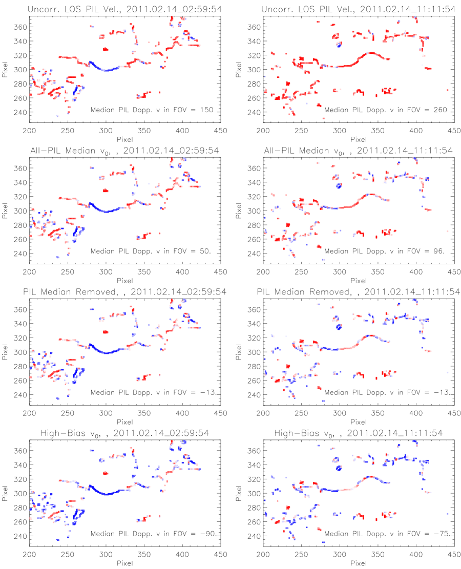
Figure 12: Examples of Doppler shifts along identified PILs in two HMI LOS magnetograms (separated by about eight hours), both without correction for the bias velocity (top row) and corrected using different estimates of $v_{0}$. Saturation in the color map is set at $\pm 250$ m/s in all panels. Second row: Doppler velocities corrected using $v_{0}$ derived by averaging over all PILs. Third row: Doppler velocities resulting by removing the median velocity on all PIL pixels. Fourth row: Doppler velocities corrected using $v_{0}$ derived by averaging over high-bias PILs, those with bias fluxes above $3.75\times 10^{17}$ Mx. Almost all PILs in the top row appear redshifted, but redshifts and blueshifts are more evenly balanced along PILs in the lower rows.

In Figure 12, we show Doppler shifts along identified PILs in two magnetograms, recorded about eight hours apart (left and right columns), both uncorrected (top row) and corrected by subtraction of different estimates of $v_{0}$ made in different ways: the average $v_{0}$ from all PILs (second row); the median Doppler velocity of all PIL pixels (third row); and the high-bias estimate of $v_{0}$, using only PILs with bias fluxes above $3.75\times 10^{17}$ Mx (fourth row). While redshifts predominate along PILs in the top row, Doppler shifts along PILs in the bottom rows are more evenly balanced between red- and blueshifts.

Our estimates of the bias velocity fall in the range of a few hundred m s^-1. Asplund & Collet (2003) used 3D, radiative MHD simulations of magnetoconvection to study line profiles for several spectral lines of iron, including some similar to HMI’s Fe I 6173 Å  line in wavelength. They find convective blue shifts similar in magnitude to our estimates of the pseudo-redshift (around 300 – 500 m/s), with uncertainties (50 – 100 m/s), similar to ours for $v_{0}$. Only $v_{0}$ estimates from high-bias PILs fall in the range found by Asplund & Collet (2003), but it should be noted that their estimate of the convective blueshift is with respect to the true rest frame, but our estimate of the bias velocity is with respect to the HMI Team’s estimate of the rest wavelength, derived from the median of 24 hours of HMI’s measured Doppler velocities within 90% of the solar radius.

We note that the equations used in our approach do depend explicitly upon spatial resolution: formally, changes in LOS flux should be consistent with up- or downflows along PILs, regardless of resolution. In practice, however, diminished spatial resolution could reduce the observable changes in unsigned LOS flux, since unresolved positive and negative LOS flux would cancel. To test the effect of spatial resolution on the method, we applied it to data in which the resolution was artificially decreased by binning pixels $(2\times 2)$. Figure 13 shows the median bias velocity at each step for each case, with dilation parameters $d=5$ pixels in both. The bias velocities were significantly correlated, with rank-order and linear correlation coefficients near 0.6. Results were very similar with $d=3$ and $d=7$ in the rebinned data. In all cases, the largest discrepancies occurred when the median FOV longitude was near 20 degrees; rebinning appears, for some reason, to affect results as central meridian distance increases.

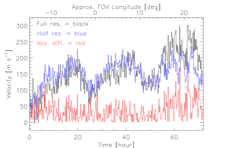
Figure 13: Bias velocities from full-resolution (black) and $(2\times 2)$-binned (blue) data are significantly correlated, with rank-order and linear correlation coefficients near 0.6. The absolute difference between the two is plotted in red; the mean and median differences are 35 m s^-1 and 29 m s^-1, respectively.

This suggests our approach is robust enough for use with data sets of different resolution. We note that median PIL Doppler velocities were very highly correlated, with with rank-order and linear correlation coefficients near 0.95, suggesting this estimator of bias velocities is very robust.

As an aside, we remark that we found Doppler structures along PILs to persist from one HMI vector magnetogram to the next, i.e., with a lifetime of at least 720 s. The lifetimes of patterns of upflows and downflows along PILs have not yet been studied yet, but bear investigation. Autocorrelation of Dopplergrams might be useful for this purpose, similar to methods used by Welsch et al. (2012).

5.1 Physical Processes Along PILs

To investigate which of our estimates for $v_{0}$ is most reasonable, we now consider the physical implications of our results in terms of the upward and downward transport of flux across the photosphere. Recall that processes that increase photospheric flux are $\Omega$-loop emergence and $U$-loop submergence, while processes that remove flux are $\Omega$-loop submergence and $U$-loop emergence. Without correcting Doppler velocities, essentially all increases and decreases in flux are attributed to the two submergence processes (from $U$-loops and $\Omega$-loops, respectively), since nearly all PILs show only redshifts. Adjusting the observed Doppler shifts to compensate for the convective blueshift, however, leads to a different apportionment between the four possible processes, depending upon the applied bias velocity: PILs that, on average, show upward transport of transverse flux and increases (decreases) in LOS flux are ascribed to $\Omega$-loop ($U$-loop) emergence, while PILs that, on average, show downward transport of transverse flux and decreases (increases) in LOS flux are ascribed to $\Omega$-loop ($U$-loop) submergence.

In Figure 14, we show the frequencies of these processes, as functions of the number of pixels along all identified PILs at all time steps, for three possible corrections: the average estimates of $v_{0}$, derived using $B_{\rm trs}$ with $B_{\rm thr}=50$ Mx cm^-2 and $d=5$ (top); the median of Doppler velocities on pixels in identified PILs (middle); and the average high-bias estimates of $v_{0}$, again using $B_{\rm trs}$ with $B_{\rm thr}=50$ Mx cm^-2 and $d=5$ (bottom). In all panels, the black curve shows the distribution of sizes of all PILs. Processes involving blueshifts ($\Omega$-loop and $U$-loop emergence) are plotted in blue, while processes involving redshifts ($\Omega$-loop and $U$-loop submergence) are plotted in red. Processes that remove flux via cancellation ($U$-loop emergence and $\Omega$-loop submergence) are plotted with dashed lines. Even with the average-$v_{0}$ correction (top panel), submergence processes still dominate, contradicting the expectation that the observed increase in unsigned radial flux of $\sim 2\times 10^{22}$ Mx over the data sequence occurred via emergence from the interior. Removing the median Doppler velocity over all pixels in identified PILs at each time step gives a more reasonable distribution of processes (middle panel): emergence and submergence processes are more closely balanced. But the requirement of a net flux increase implies that emerging processes should predominate, and this expectation is only consistent with the high-bias-$v_{0}$ correction (bottom panel).

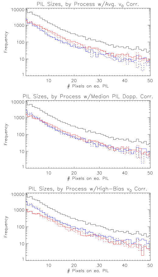
Figure 14: Frequencies of emergence and submergence processes, as functions of the number of pixels along all identified PILs at all time steps, for three possible corrections to Doppler velocities: the average estimates of $v_{0}$, derived using $B_{\rm trs}$ with $B_{\rm thr}=50$ Mx cm^-2 and $d=5$ (top); the median of Doppler velocities on pixels in identified PILs (middle); and the average high-bias estimates of $v_{0}$, again using $B_{\rm trs}$ with $B_{\rm thr}=50$ Mx cm^-2 and $d=5$ (bottom). In all panels, the black curve shows the distribution of sizes of all PILs. Processes involving blueshifts ($\Omega$-loop and $U$-loop emergence) are plotted in blue, while processes involving redshifts ($\Omega$-loop and $U$-loop submergence) are plotted in red. Processes that remove flux via cancellation ($U$-loop emergence and $\Omega$-loop submergence) are plotted with dashed lines.

In principle, observations of changes in total unsigned radial flux in the FOV should be consistent, separately, with estimates of changes in LOS flux near PILs and the upward / downward transport of transverse flux. Our estimates of flux increase by $\Omega$-loop emergence from changes in LOS flux near PILs are roughly consistent with the net change in LOS flux over the entire sequence. Unfortunately, other components of our flux budgeting near PILs are inaccurate, in two ways.

First, our estimates of flux removed by cancellation processes ($\Omega$-loop submergence and $U$-loop emergence) are too large (from $\sim 10^{22}$ Mx to several times this), whether inferred from LOS changes or rates of transport of transverse flux. This might be explained if some flux is dispersing near PILs that we identify as sites of cancellation, instead of submerging/emerging at these PILs. As discussed in Section 4.2, identifying magnetogram features and tracking their evolution (DeForest et al., 2007), or imposing additional constraints (e.g., requiring cancellation to persist for multiple time steps, or taking the flux lost to be the minimum of that among the two polarities; see Welsch et al. 2011) could more accurately quantify canceled flux. We leave investigation of these approaches for future work.

Second, our estimated rates of transport of transverse flux are systematically too large compared to changes in LOS flux near PILs, for all processes. As noted in Section 4.2 above, inaccuracies in PIL identification could incorporate velocities from siphon flows in our flux transport rates. In addition, a filling factor $f<1$ could also play a role, since it would affect $|\Delta\Phi_{\rm LOS}|$ and $|\Delta\Phi_{vBL}|$ differently: while length transverse to the LOS (two factors of which enter computation of $|\Delta\Phi_{LOS}|$) is scaled by $\sqrt{f}$, length along the LOS (which enters computation of $|\Delta\Phi_{vBL}|$) is not. Hence, if $f<1$, one would expect $|\Delta\Phi_{vBL}|>|\Delta\Phi_{\rm LOS}|$. Given typical discrepancies in fluxes by factors of 4 – 6, this would imply filling factors of $\sim 0.05$. This would be implausible in umbrae, where the field is expected to be space-filling. We analyze PILs, however, which are, almost as a matter of definition, in mixed-polarity regions, where the field is expected to be more intermittent. The plausibility of a filling factor this small along PILs is unclear.

Another possibility is that flux transport rates are overestimated because the transport is not ideal, i.e., that the plasma is moving at a different speed than the flux transport rate. For instance, if the flux emergence process were not ideal (Pariat et al., 2004), then the rate of flux transport derived from Doppler shifts would underestimate the true emergence rate, since flux would be partially decoupled from the plasma, allowing flux to move upward independently of the plasma. While magnetic diffusivity would be manifested in that case by flux slipping through stationary (or much slower-moving) plasma at a rate faster than that suggested by ideal transport, the ideal transport rate is too high in our estimates. Chae et al. (2008) note that turbulent diffusivity can act on canceling LOS magnetic fluxes; but again, we find the rate of loss of LOS field to be too small relative to ideal transport of horizontal fields, and invoking turbulent diffusivity would make this discrepancy worse. One possible explanation is that unmagnetized plasma, which could be systematically faster-moving than magnetized plasma, could be contributing significantly to Doppler signal.

To quantitatively characterize cases of apparently non-ideal evolution, one could employ a simple non-ideal model, assuming a uniform magnetic diffusivity $\eta$ is present. This would imply a corresponding non-ideal electric field parallel to the PIL (in addition to the ideal electric field along the PIL already used to estimate $\Delta\Phi_{vBL}$), given by

$$cE_{\parallel}^{\rm NI}=\eta|\partial_{\rm LOS}B_{\perp}-\partial_{\perp}B_{\rm LOS}|~{},$$ (33)

where, as above, $\,\hat{\mathbf{x}}_{\perp}$ locally points across the PIL (see equation 10). For PILs where $|\Delta\Phi_{\rm LOS}|\gg|\Delta\Phi_{vBL}|$, we could attribute the excess $\Delta\Phi_{\rm LOS}$ to $\eta\,\partial_{\perp}B_{\rm LOS}$ integrated along the PIL, taking $\partial_{\rm LOS}B_{\perp}$ to be negligible, as it would be if there were a current sheet along the PIL (e.g., Litvinenko 1999). Values of $\eta$ derived this way could be compared to the assumed values used by Litvinenko (1999), Chae et al. (2002), and Litvinenko et al. (2007). For PILs where $|\Delta\Phi_{\rm LOS}|\ll|\Delta\Phi_{vBL}|$, we could attribute the excess $\Delta\Phi_{vBL}$ to overestimation of the transport rate of transverse flux along the LOS, due to slippage of transverse flux through the moving plasma in the presence of diffusivity. Because $\partial_{\rm LOS}B_{\perp}$ is unknown for such cases, however, we could not estimate $\eta$.

We note that spurious changes in LOS fields over a magnetogram FOV, due, e.e., to artifacts arising from orbital motion in the case of HMI (or any other cause) will introduce errors into the bias velocity estimate: our approach attributes changes in unsigned LOS flux to emergence / submergence, so changes unrelated to actual emergence / submergence will introduce error. Are the known artifacts in HMI field strengths significant? Probably not, since the orbital variations occur on timescales much slower than the evolution over $\Delta t=$ 24 min. that we analyze. Liu et al. (2012a) report changes in mean $|B_{\rm LOS}|$ of approx. 150 Mx cm^-2 peak to peak, i.e., over 12 hr. (see their Figure 5). This rate of change corresponds to a change of 5 Mx cm^-2 over 24 min., which is at the noise level of an individual LOS measurement. This implies these slow variations in LOS field strength would be dominated by fluctuations from noise, or faster evolution.

5.2 Empirical Estimates of Uncertainties

After filtering azimuths and removing Doppler velocities due to solar rotation and convection, we interpolated the data to sub-pixel accuracy for two purposes: (i) image co-registration, to remove frame-to-frame jitter, primarily from quantized changes in the cutout window boundaries (determined by pixel size) imposed on the smooth rotation of the underlying solar features; and (ii) Mercator projection of the spherical data onto a uniform grid in a Cartesian frame. While interpolation propagates errors from pathological pixels, and can introduce other artifacts (e.g., smoothing) into the data, it should nonetheless be undertaken, since significant whole-frame shifts were found (some frame-to-frame shifts were on the order of 1 pixel, and cumulative shifts showed both secular evolution and jumps) in the $x$ and $y$ directions by Fourier cross-correlation in the $B_{\rm LOS}$ image sequence.

Since azimuth filtering and interpolation modify the input data, we characterized uncertainties in the dataset empirically, instead of relying upon error arrays produced in the HMI processing pipeline. To do so, we constructed histograms of the LOS and transverse fields, $B_{\rm LOS}$ and $B_{\rm trs}$ respectively, at each time step, and statistically characterized these distributions.

In each distribution of $B_{\rm LOS}$, we interpret the weak-field core of distribution as a measure of noise (e.g., DeForest et al. 2007), which we quantified by fitting the core of the distribution ($\pm 6$ Mx cm^-2) with a Gaussian of width $\sigma_{\rm L}$, and by finding the flux density at half max (HM) in the left and right wings. Statistically, the mean and standard deviation of fitted $\sigma_{\rm L}$’s were $4.1\pm 0.3$ Mx cm^-2 and combined left- and right-widths at HM were $4.7\pm 0.5$ Mx cm^-2, but fluctuations with a periodicity around $6$ hours were observed. In SDO’s geosynchronous orbit, (i) Doppler motion toward and away from the Sun and (ii) thermal cycling due to the Earth’s day-side albedo would both exhibit 12-hour periodicities, and would be a quarter cycle out of phase, so could combine to produce variations in instrumental response with such a characteristic 6-hour periodicity. This analysis roughly agrees with the HMI Team’s estimate of the uncertainty of $6$ Mx cm^-2, and suggests that the uncertainty in the LOS field component assumed above, 20 Mx cm^-2, probably overestimates the true uncertainty.

Since $B_{\rm trs}$ is a magnitude, it is necessarily positive, and we find the distribution peaked away from zero. If the distributions of each of the three observed field components were Gaussian, with the same width $\sigma$, then the distribution of transverse field strengths would be that of a 3D Maxwell distribution, $\propto B_{\rm trs}^{2}\exp(-B_{\rm trs}^{2}/2\sigma^{2})$. In fact, we find that a Gaussian displaced from zero (fitted to data within $\pm 25$ Mx cm^-2 of the tallest peak) consistently fit each distribution of $B_{\rm trs}$ more closely (as quantified by $\chi^{2}$ over the whole distribution) than a 3D (or 2D) Maxwellian. It should be noted, however, that the shape of the distribution varied substantially over the observing sequence — e.g., exhibiting two peaks at some time steps — so the Gaussian fits, although better than the Maxwellians, were still poor in many cases. The means and standard deviations of the Gaussians’ fitted centroids $B_{\rm t0}$ and widths $\sigma_{\rm t}$ were $81\pm 17$ Mx cm^-2 and $29\pm 6$ Mx cm^-2, respectively. Both also exhibited periodicities, though with more complicated temporal structure than with fits to the distribution of $B_{\rm LOS}$, with the clearest period at $\sim 24$ hr. This analysis suggests that our assumed uncertainty in the transverse field component, 90 Mx cm^-2, is reasonable.

6 Summary

We have demonstrated a technique to estimate any spatially-constant bias velocity $v_{0}$ present in measured photospheric Doppler velocities using a sequence of observations of the vector magnetic field near disk center. Such biases can arise from instrumental effects (e.g., thermal variations in instrument components) or from the convective blueshift (Dravins et al., 1981). Our technique uses consistency between changes in LOS flux near PILs close to disk center and the transport of transverse flux implied by Doppler velocities along those PILs.

We also noted that an estimate of the bias velocity can be made more simply, from the median of Doppler velocities along all pixels in LOS PILs close to disk center. This approach does not require measurement of the transverse field; only an LOS magnetogram and a Dopplergram are required. One need only identify PILs, and take the median Doppler velocity on all PIL pixels. While this approach ignores our flux-matching constraint in equation (18), and could therefore, in principle, be biased by a strong episode of flux emergence or submergence, we only found evidence of a very weak bias.

Accurately calibrated Doppler velocities can be used to better understand photospheric dynamics prior to and during CMEs (Schuck, 2010), to improve estimates of the photospheric electric field and thereby estimate the photospheric Poynting flux (Fisher et al., 2012), and to differentiate between possible mechanisms of flux cancellation ($\Omega$-loop submergence, U-loop emergence, or reconnective cancellation).

For the HMI dataset we studied, we found clear evidence of bias velocities, though estimates of $v_{0}$ ranged from less than 100 m s^-1 to $\sim 500$ m s^-1 over the course of the run. Only the larger estimates of $v_{0}$ — in the range of 350 $\pm$ 85 m s^-1 — were consistent with a majority of PILs being sites of emergence, in accordance with the substantial increase in total unsigned magnetic flux over the duration of our data set.

Unfortunately, flux budgets based upon our estimates of the rates of emergence and submergence are very noisy, and likely subject to large errors. Consequently, improving our approach to constraining the bias velocity, or identifying new constraints, would be desirable. We plan a careful investigation of systematic sources of uncertainty in our method (e.g., better quantitative characterization of flux cancellation and changes in LOS fluxes near PILs), or possible bias (e.g., greater errors in shorter vs. longer PILs, or weak-field vs. strong-field PILs).

It would also be worthwhile to compare results of our electromagnetic calibration with calibrations based upon fitting the center-to-limb component of full-disk HMI measurements of Doppler velocities (Snodgrass, 1984; Hathaway, 1992; Hathaway et al., 2000; Schuck, 2010). As noted above, center-to-limb fitting has a major physical uncertainty: the physics of the center-to-limb variation in Doppler shift in the particular spectral line used by HMI (or any other spectral line) involves detailed interactions between height of formation, the height of convective turnover, the variation with viewing angle of the average convective flow speed, and the variation with viewing angle of optical depth (Carlsson et al., 2004). Diverging flows tangent to the photosphere in granules can, depending upon optical depth in granules at the formation height of the line, produce a convective blueshift toward the limb (e.g., Takeda & Ueno 2012), because diverging flows on the near sides of granules approach the viewer, while receding flows on the far sides of the granules are at least partially obscured by the optical depth of the granules (see Figure 2). Hence, finding the center-to-limb shift in a line does not imply that the line does not still possess an overall additional shift.

We note that, in addition to the Dopplergram data analyzed here, the HMI Team also produces independent estimates of Doppler velocities in the Milne-Eddington inversion process. While comparisons between ME and Dopplergram velocities show them to be quite similar (Yang Liu, private communication 2011), these independent measurements can provide additional information, e.g., better characterization of uncertainties.

In addition, as a step in our data reduction, we implemented a procedure to correct a few episodes of single-frame fluctuations in the direction of the transverse magnetic field vector, by nearly 180^∘. We attributed these flips-followed-by-reversals to errors in resolution of the 180^∘ ambiguity in the transverse field. As discussed in further detail above, our automated procedure reverses suspicious transient flips by imposing temporal continuity: among pixels with jumps in azimuth larger than 120^∘ at frame $i$, it reverses any azimuths that increase the average of the four unsigned differences in azimuth between frame $i$ and the nearest $\pm 2$ frames. This relatively simple algorithm corrected the episodes of suspicious azimuth changes that we noticed.

Appendix A Geometric Effects Away from Disk Center

We have asserted that the calibration method we describe here is only valid near disk center. To better understand why, we consider a particular configuration of emerging magnetic flux in Figure 15, where it is illustrated in two different orientations with respect to the viewer. This configuration is highly idealized: we assume the configuration is invariant in the direction into the page, and that emerging field lines have the same shape as field lines that have already emerged. In both panels, the viewer is assumed to look down from above the top of the figure.

In the upper left panel, a plane tangent to the photosphere at the radial-field PIL is normal to the LOS. At this particular viewing angle, the photospheric normal direction and the LOS coincide. Away from the PIL, the field is uniformly tilted from the LOS by the inclination angle $\Theta=45^{\circ}.$ In the upper right panel, the normal to the plane tangent to the photosphere at the radial-field PIL is tilted with respect to the LOS by an angle $\theta=45^{\circ}$, which is also the tilt of the legs of the emerging flux system with respect to the photosphere.

We assume the flux emergence is ideal, such that the electric field obeys equation (3), and flux is therefore frozen to the plasma. The rate of flux emergence by a radial flow can therefore be inferred from observations of the upper-left panel in two ways: (1) from the increase in the the total unsigned LOS flux (the integrated absolute value of the curve plotted in the lower left panel); and (2) from the product of the transverse field at the PIL and the Doppler signal at the PIL. The equivalence of these measures of the rate ideal flux emergence underlies the Doppler calibration method presented in this paper: we assume any inconsistency between (1) and (2) is due to a bias in the Doppler zero point.

In contrast, flux emergence can only be unambiguously inferred by observations of the upper right panel one way: from the increase in the the total unsigned flux (either LOS flux or radial flux). This is because the magnetic field at the radial-field PIL has a component along the LOS, implying Doppler shifts at this PIL might contain a contribution from flows parallel to ${\mathbf{B}}$ there. Flows parallel to ${\mathbf{B}}$, however, do not drive flux emergence, and cannot be distinguished from Doppler shifts due to flows perpendicular to ${\mathbf{B}}$.

It is also clear that the relative orientation of the negative-polarity flux and the LOS implies that an observer would not see an increase in negative-polarity LOS flux as emergence proceeds. Hence, observations of the emergence of tilted flux in LOS magnetograms can exhibit strong flux imbalance. Measurements of changes in the radial flux, from vector magnetograms, would be balanced in this idealized case.

Figure 15: Upper left and right panels depict a highly idealized emerging flux configuration, assumed to be invariant in the direction into the page, viewed in two different orientations with respect to an observer, who is assumed to be looking down from above the top of this figure. In the upper left panel, measurements of Doppler velocities on the radial-field PIL and transverse fields at the PIL can be used to infer the rate of flux emergence. In the upper right panel, the magnetic field at the radial-field PIL has a component along the LOS, so flows parallel to ${\mathbf{B}}$ (which do not drive flux emergence) can contribute to Doppler shifts, implying the Doppler velocity cannot unambiguously determine the rate of flux emergence at this PIL. In both cases, flux emergence can be detected from increases in total unsigned LOS flux (the curves plotted in the bottom left and right panels), and quantitatively estimated from changes in the total unsigned radial magnetic flux.

References

- Abbett (2007) Abbett, W. P. 2007, ApJ, 665, 1469
- Asplund & Collet (2003) Asplund, M. & Collet, R. 2003, in Astronomical Society of the Pacific Conference Series, Vol. 293, 3D Stellar Evolution, ed. S. Turcotte, S. C. Keller, & R. M. Cavallo, 197–+
- Bellot Rubio & Beck (2005) Bellot Rubio, L. R. & Beck, C. 2005, ApJ, 626, L125
- Berger et al. (2007) Berger, T. E., Rouppe van der Voort, L., & Löfdahl, M. 2007, ApJ, 661, 1272
- Carlsson et al. (2004) Carlsson, M., Stein, R. F., Nordlund, Å., & Scharmer, G. B. 2004, ApJ, 610, L137
- Cavallini et al. (1986) Cavallini, F., Ceppatelli, G., & Righini, A. 1986, A&A, 163, 219
- Chae (2001) Chae, J. 2001, ApJ, 560, L95
- Chae et al. (2008) Chae, J., Litvinenko, Y. E., & Sakurai, T. 2008, ApJ, 683, 1153
- Chae et al. (2004) Chae, J., Moon, Y., & Pevtsov, A. A. 2004, ApJ, 602, L65
- Chae et al. (2002) Chae, J., Moon, Y., Wang, H., & Yun, H. S. 2002, Sol. Phys., 207, 73
- Démoulin & Berger (2003) Démoulin, P. & Berger, M. A. 2003, Sol. Phys., 215, 203
- DeForest et al. (2007) DeForest, C. E., Hagenaar, H. J., Lamb, D. A., Parnell, C. E., & Welsch, B. T. 2007, ApJ, 666, 576
- Dravins et al. (1981) Dravins, D., Lindegren, L., & Nordlund, A. 1981, A&A, 96, 345
- Falconer et al. (2003) Falconer, D. A., Moore, R. L., & Gary, G. A. 2003, Journal of Geophysical Research (Space Physics), 108, 1380
- Fisher & Welsch (2008) Fisher, G. H. & Welsch, B. T. 2008, in Astronomical Society of the Pacific Conference Series, Vol. 383, Subsurface and Atmospheric Influences on Solar Activity, ed. R. Howe, R. W. Komm, K. S. Balasubramaniam, & G. J. D. Petrie, 373–380; also arXiv:0712.4289
- Fisher et al. (2012) Fisher, G. H., Welsch, B. T., & Abbett, W. P. 2012, Sol. Phys., 277, 153
- Fisher et al. (2010) Fisher, G. H., Welsch, B. T., Abbett, W. P., & Bercik, D. J. 2010, ApJ, 715, 242
- Fleck et al. (2011) Fleck, B., Couvidat, S., & Straus, T. 2011, Sol. Phys., 271, 27
- Gaizauskas et al. (1983) Gaizauskas, V., Harvey, K. L., Harvey, J. W., & Zwaan, C. 1983, ApJ, 265, 1056
- Gray (2009) Gray, D. F. 2009, ApJ, 697, 1032
- Hagenaar et al. (2003) Hagenaar, H. J., Schrijver, C. J., & Title, A. M. 2003, ApJ, 584, 1107
- Harvey et al. (2007) Harvey, J. W., Branston, D., Henney, C. J., Keller, C. U., & the SOLIS and GONG Teams. 2007, ApJL, 659, L177
- Harvey et al. (1999) Harvey, K. L., Jones, H. P., Schrijver, C. J., & Penn, M. J. 1999, Solar Phys., 190, 35
- Hathaway (1992) Hathaway, D. H. 1992, Sol. Phys., 137, 15
- Hathaway et al. (2000) Hathaway, D. H., Beck, J. G., Bogart, R. S., Bachmann, K. T., Khatri, G., Petitto, J. M., Han, S., & Raymond, J. 2000, Solar Phys., 193, 299
- Iida et al. (2010) Iida, Y., Yokoyama, T., & Ichimoto, K. 2010, ApJ, 713, 325
- Keller et al. (2003) Keller, C. U., Harvey, J. W., & Giampapa, M. S. 2003, in SPIE Conference, Vol. 4853, Innovative Telescopes and Instrumentation for Solar Astrophysics. Edited by Stephen L. Keil, Sergey V. Avakyan., ed. S. L. Keil & S. V. Avakyan, 194–204
- Kosugi et al. (2007) Kosugi, T., Matsuzaki, K., Sakao, T., Shimizu, T., Sone, Y., Tachikawa, S., Hashimoto, T., Minesugi, K., Ohnishi, A., Yamada, T., Tsuneta, S., Hara, H., Ichimoto, K., Suematsu, Y., Shimojo, M., Watanabe, T., Shimada, S., Davis, J. M., Hill, L. D., Owens, J. K., Title, A. M., Culhane, J. L., Harra, L. K., Doschek, G. A., & Golub, L. 2007, Sol. Phys., 243, 3
- Kubat & Karlicky (1986) Kubat, J. & Karlicky, M. 1986, Bulletin of the Astronomical Institutes of Czechoslovakia, 37, 155
- Kubo et al. (2008) Kubo, M., Lites, B. W., Shimizu, T., & Ichimoto, K. 2008, ApJ, 686, 1447
- Kubo & Shimizu (2007) Kubo, M. & Shimizu, T. 2007, ApJ, 671, 990
- Kusano et al. (2002) Kusano, K., Maeshiro, T., Yokoyama, T., & Sakurai, T. 2002, ApJ, 577, 501
- Lamb et al. (2008) Lamb, D. A., DeForest, C. E., Hagenaar, H. J., Parnell, C. E., & Welsch, B. T. 2008, ApJ, 674, 520
- Leka et al. (2009) Leka, K. D., Barnes, G., & Crouch, A. 2009, in Astronomical Society of the Pacific Conference Series, Vol. 415, The Second Hinode Science Meeting: Beyond Discovery-Toward Understanding, ed. B. Lites, M. Cheung, T. Magara, J. Mariska, & K. Reeves, 365
- Lin & Rimmele (1999) Lin, H. & Rimmele, T. 1999, ApJ, 514, 448
- Lites et al. (1995) Lites, B. W., Low, B. C., Martinez Pillet, V., Seagraves, P., Skumanich, A., Frank, Z. A., Shine, R. A., & Tsuneta, S. 1995, ApJ, 446, 877
- Litvinenko (1999) Litvinenko, Y. E. 1999, ApJ, 515, 435
- Litvinenko et al. (2007) Litvinenko, Y. E., Chae, J., & Park, S. 2007, ApJ, 662, 1302
- Liu et al. (2012a) Liu, Y., Hoeksema, J. T., Scherrer, P. H., Schou, J., Couvidat, S., Bush, R. I., Duvall, T. L., Hayashi, K., Sun, X., & Zhao, X. 2012a, Sol. Phys., 279, 295
- Liu et al. (2012b) Liu, Y., Scherrer, P. H., Hoeksema, J. T., Schou, J., Bai, T., Beck, J. G., Bobra, M., Bogart, R. S., Bush, R. I., Couvidat, S., Hayashi, K., Kosovichev, A. G., Larson, T. P., Rabello-Soares, C., Sun, X., Wachter, R., Zhao, J., Zhao, X. P., Duvall, Jr., T. L., DeRosa, M. L., Schrijver, C. J., Title, A. M., Centeno, R., Tomczyk, S., Borrero, J. M., Norton, A. A., Barnes, G., Crouch, A. D., Leka, K. D., Abbett, W. P., Fisher, G. H., Welsch, B. T., Muglach, K., Schuck, P. W., Wiegelmann, T., Turmon, M., Linker, J. A., Mikić, Z., Riley, P., & Wu, S. T. 2012b, in Astronomical Society of the Pacific Conference Series, Vol. 455, 4th Hinode Science Meeting: Unsolved Problems and Recent Insights, ed. L. Bellot Rubio, F. Reale, & M. Carlsson, 337
- Livi et al. (1985) Livi, S. H. B., Wang, J., & Martin, S. F. 1985, Australian Journal of Physics, 38, 855
- Low (2001) Low, B. C. 2001, JGR, 106, 25141
- Martens & Zwaan (2001) Martens, P. C. & Zwaan, C. 2001, ApJ, 558, 872
- Metcalf et al. (1995) Metcalf, T. R., Jiao, L., McClymont, A. N., Canfield, R. C., & Uitenbroek, H. 1995, ApJ, 439, 474
- Okamoto et al. (2008) Okamoto, T. J., Tsuneta, S., Lites, B. W., Kubo, M., Yokoyama, T., Berger, T. E., Ichimoto, K., Katsukawa, Y., Nagata, S., Shibata, K., Shimizu, T., Shine, R. A., Suematsu, Y., Tarbell, T. D., & Title, A. M. 2008, ApJ, 673, L215
- Pariat et al. (2004) Pariat, E., Aulanier, G., Schmieder, B., Georgoulis, M. K., Rust, D. M., & Bernasconi, P. N. 2004, ApJ, 614, 1099
- Rabin et al. (1984) Rabin, D., Moore, R., & Hagyard, M. J. 1984, ApJ, 287, 404
- Rieutord et al. (2001) Rieutord, M., Roudier, T., Ludwig, H.-G., Nordlund, Å., & Stein, R. 2001, A&A, 377, L14
- Sánchez Almeida (2009) Sánchez Almeida, J. 2009, Ap&SS, 320, 121
- Scherrer et al. (2012) Scherrer, P. H., Schou, J., Bush, R. I., Kosovichev, A. G., Bogart, R. S., Hoeksema, J. T., Liu, Y., Duvall, T. L., Zhao, J., Title, A. M., Schrijver, C. J., Tarbell, T. D., & Tomczyk, S. 2012, Sol. Phys., 275, 207
- Schou et al. (2012) Schou, J., Scherrer, P. H., Bush, R. I., Wachter, R., Couvidat, S., Rabello-Soares, M. C., Bogart, R. S., Hoeksema, J. T., Liu, Y., Duvall, T. L., Akin, D. J., Allard, B. A., Miles, J. W., Rairden, R., Shine, R. A., Tarbell, T. D., Title, A. M., Wolfson, C. J., Elmore, D. F., Norton, A. A., & Tomczyk, S. 2012, Sol. Phys., 275, 229
- Schrijver (2007) Schrijver, C. J. 2007, ApJ, 655, L117
- Schrijver et al. (1997) Schrijver, C. J., Title, A. M., van Ballegooijen, A. A., Hagenaar, H. J., , & Shine, R. A. 1997, ApJ, 487, 424
- Schuck (2006) Schuck, P. W. 2006, ApJ, 646, 1358
- Schuck (2008) —. 2008, ApJ, 683, 1134
- Schuck (2010) —. 2010, ApJ, 714, 68
- Snodgrass (1983) Snodgrass, H. 1983, ApJ, 270, 288
- Snodgrass (1984) —. 1984, Solar Phys., 94, 13
- Spruit et al. (1987) Spruit, H. C., Title, A. M., & van Ballegooijen, A. A. 1987, Sol. Phys., 110, 115
- Sun et al. (2012) Sun, X., Hoeksema, J. T., Liu, Y., Wiegelmann, T., Hayashi, K., Chen, Q., & Thalmann, J. 2012, ApJ, 748, 77
- Takeda & Ueno (2012) Takeda, Y. & Ueno, S. 2012, Sol. Phys., 281, 551
- Tsuneta et al. (2008) Tsuneta, S., Ichimoto, K., Katsukawa, Y., Nagata, S., Otsubo, M., Shimizu, T., Suematsu, Y., Nakagiri, M., Noguchi, M., Tarbell, T., Title, A., Shine, R., Rosenberg, W., Hoffmann, C., Jurcevich, B., Kushner, G., Levay, M., Lites, B., Elmore, D., Matsushita, T., Kawaguchi, N., Saito, H., Mikami, I., Hill, L. D., & Owens, J. K. 2008, Sol. Phys., 249, 167
- van Ballegooijen (2008) van Ballegooijen, A. A. 2008, in Astronomical Society of the Pacific Conference Series, Vol. 383, Subsurface and Atmospheric Influences on Solar Activity, ed. R. Howe, R. W. Komm, K. S. Balasubramaniam, & G. J. D. Petrie , 191–+
- van Ballegooijen & Mackay (2007) van Ballegooijen, A. A. & Mackay, D. H. 2007, ApJ, 659, 1713
- van Driel-Gesztelyi et al. (2000) van Driel-Gesztelyi, L., Malherbe, J.-M., & Démoulin, P. 2000, A&A, 364, 845
- Wallenhorst & Howard (1982) Wallenhorst, S. G. & Howard, R. 1982, Sol. Phys., 76, 203
- Wallenhorst & Topka (1982) Wallenhorst, S. G. & Topka, K. P. 1982, Sol. Phys., 81, 33
- Welsch (2006) Welsch, B. T. 2006, ApJ, 638, 1101
- Welsch et al. (2007) Welsch, B. T., Abbett, W. P., DeRosa, M. L., Fisher, G. H., Georgoulis, M. K. Kusano, K., Longcope, D. W., Ravindra, B., & Schuck, P. W. 2007, ApJ, 670, 1434
- Welsch et al. (2011) Welsch, B. T., Christe, S., & McTiernan, J. M. 2011, Sol. Phys., 274, 131
- Welsch et al. (2004) Welsch, B. T., Fisher, G. H., Abbett, W. P., & Régnier, S. 2004, ApJ, 610, 1148
- Welsch et al. (2012) Welsch, B. T., Kusano, K., Yamamoto, T. T., & Muglach, K. 2012, ApJ, 747, 130
- Welsch & Li (2008) Welsch, B. T. & Li, Y. 2008, in Astronomical Society of the Pacific Conference Series, Vol. 383, Subsurface and Atmospheric Influences on Solar Activity, ed. R. Howe, R. W. Komm, K. S. Balasubramaniam, & G. J. D. Petrie, 429–437; also arXiv:0710.0562
- Welsch et al. (2009) Welsch, B. T., Li, Y., Schuck, P. W., & Fisher, G. H. 2009, ApJ, 705, 821
- Yurchyshyn & Wang (2001) Yurchyshyn, V. B. & Wang, H. 2001, Sol. Phys., 202, 309